A Framework of Runge–Kutta, Discontinuous Galerkin, Level Set and Direct Ghost Fluid Methods for the Multi-Dimensional Simulation of Underwater Explosions

Abstract

This work describes the development of a hybrid framework of Runge–Kutta (RK), discontinuous Galerkin (DG), level set (LS) and direct ghost fluid (DGFM) methods for the simulation of near-field and early-time underwater explosions (UNDEX) in early-stage ship design. UNDEX problems provide a series of challenging issues to be solved. The multi-dimensional, multi-phase, compressible and inviscid fluid-governing equations must be solved numerically. The shock front in the solution field must be captured accurately while maintaining the total variation diminishing (TVD) properties. The interface between the explosive gas and water must be tracked without letting the numerical diffusion across the material interface lead to spurious pressure oscillations and thus the failure of the simulation. The non-reflecting boundary condition (NRBC) must effectively absorb the wave and prevent it from reflecting back into the fluid. Furthermore, the CFD solver must have the capability of dealing with fluid–structure interactions (FSI) where both the fluid and structural domains respond with significant deformation. These issues necessitate a hybrid model. In-house CFD solvers (UNDEXVT) are developed to test the applicability of this framework. In this development, code verification and validation are performed. Different methods of implementing non-reflecting boundary conditions (NRBCs) are compared. The simulation results of single and multi-dimensional cases that possess near-field and early-time UNDEX features—such as shock and rarefaction waves in the fluid, the explosion bubble, and the variation of its radius over time—are presented. Continuing research on two-way coupled FSI with large deformation is introduced, and together with a more complete description of the direct ghost fluid method (DGFM) in this framework will be described in subsequent papers.

1. Introduction

In an underwater explosion, a series of events occur sequentially, including ignition, the chemical reaction of explosives, the generation and spreading of a shock wave outwards and a rarefaction wave inwards, the interaction between the shock wave and near-by structures, local and bulk cavitation in the fluid, the explosive bubble expanding and contracting, multiple bubble pulses being generated due to it, the interaction between the bubble pulses and nearby structures, reflected waves from either the structures or the free surface and their interaction with bubble, and bubble jetting, etc. The structure experiences primary shock wave loading and deformation, the collapse of the local cavitation and reloading exerted by the fluid, loading caused by bubble pulses and bubble jetting which leads to further deformation, whipping, and other global and dynamic responses [1,2,3,4].

Due to this complexity in the physics of an underwater explosion, it is reasonable to focus the research of UNDEX on separate aspects of the problem based on the occurrence times and timescales of the problem, i.e., early-time and late-time. It is also common in practice to separate the research based on the spatial characteristics, i.e., far-field and near-field [5,6,7]. This work is carried out with a focus on near-field and early-time UNDEX. Events including the shock and rarefaction waves, the reflection of the shock waves and their interaction with the fluid, the variation of the explosive bubble size and structural deformation, and its interaction with fluid, etc., are also problems of interest in this category [5].

Features of near-field and early-time UNDEX indicate that there are a series of challenging tasks to be solved. First, almost all aspects of an UNDEX event must be considered. Detail is important. This means that models with too many assumptions—such as linear acoustic wave equations that just model the shock pressure [2], bubble models derived from potential flow theory that deal only with the explosive bubble [8], the Rayleigh–Plesset equations that govern only the dynamics of spherical bubbles [9,10], or empirical models such as the similitude equations that assume only one-way effects from the fluid to the structure [1,11]—are not sufficient in the near-field and early-time UNDEX simulation. The necessary mathematical problems to be solved are the compressible and inviscid Navier–Stokes equations, i.e., the Euler equations. Second, the explosive is relatively close to the structural object in near-field UNDEX. Because of this, the explosive gas bubble of extremely high pressure created by the detonation of the explosive charge may interact directly with the structure, and must be fully inside of the modeled numerical fluid domain. The fluid problem to be solved is thus multi-phase. The simulation of the explosive bubble, especially the variation of its radius over time, also requires a multi-phase CFD simulation. Third, the discontinuities in the solution field, especially the shock front, must be tracked accurately while the total variation diminishing property is ensured. This is achieved by a generalized slope limiter with a small adjustment made to better work with the discretization of the fluid-governing equations [5,12]. Fourth, given the memory-consuming nature of a full CFD and FSI simulation, a smaller fluid domain is preferred in order to save computing memory and make the simulation computationally manageable. An effective imposition of a non-reflecting boundary condition is thus essential in the building of this hybrid framework of algorithms [13]. The NRBC must effectively absorb the shockwave and prevent it from reflecting back into the fluid, so that the computational domain does not need to be extremely large. This is even more important as the simulation runs longer, for example, in order to capture the simulation of the bubble radius and its variation over time. Finally, the structure and fluid deform significantly in a near-field UNDEX. Unlike most related works in the literature that use a body-conforming fluid mesh so that both the fluid domain and mesh are dynamic throughout the FSI simulation, e.g., the arbitrary Lagrangian–Eulerian (ALE) algorithm [14], this work uses the embedded boundary method so that the fluid mesh is fixed in space but can follow the structural deformation [15]. In summary, the highlights of this paper are:

(1)

Documenting a straightforward method for the multi-dimensional discretization of compressible and inviscid fluid-governing equations (the Euler equations) using a modal DG method.

(2)

Performing order-of-accuracy verification on single and multi-dimensional solvers with different formal orders of accuracy.

(3)

Proving the applicability of this hybrid framework by the simulation results of multiple cases that possess near-field and early-time UNDEX features, as well as their comparison with analytic solutions, experiments and simulations using other numerical methods.

(4)

Comparing different methods for enforcing NRBC, developing a new method of enforcing the NRBC, and selecting this method as an optimized method.

(5)

FSI simulation of near-field and early-time UNDEX can be performed once this hybrid framework is coupled with the embedded boundary method (EBM).

This paper and the following paper [16] present the development of a hybrid framework of Runge–Kutta (RK), discontinuous Galerkin (DG), level set (LS) and direct ghost fluid methods (DGFM) methods to address these issues. The second paper will focus on the direct ghost fluid method (DGFM). In this hybrid framework, multi-dimensional, multi-phase, compressible and inviscid fluid-governing equations, i.e., the Euler equations, are solved numerically using the Runge–Kutta method as the time marching scheme, the discontinuous Galerkin method as the spatial discretization scheme, the level set method to track the material interface between explosive gas and water with the help of the direct ghost fluid method [5], and the embedded boundary method so that the fluid solver is capable of simulating the fluid with large deformation.

2. Survey of Related Work

Efforts to model near-field UNDEX using CFD were made as early as the 1980s. One-dimensional modeling and simulation were performed first. Flores used a 1D spherical fluid-governing equation as the mathematical model, and solved it using Glimm’s method [17]. Cocchi applied a Godunov-type prediction–correction method in the algorithm so that property values at the gas–water interface were effectively corrected [18]. The application of this method was able to use analytical solutions of 1D Riemann problems when the equations of the state of both the explosive gas and the surrounding water were modeled as ideal [19]. The analytical solution of the one-dimensional shock tube problem provided a better understanding of the physics of the shock wave, the rarefaction wave and the movement of the material interface between the two phases.

Research was extended to the multi-dimensional modeling and simulation of UNDEX as more progress was made with algorithms such as the finite volume method (FVM), finite element method (FEM) and discontinuous Galerkin (DG) method. The finite volume method is the most frequently used approach for fluid discretization. Farhat et al. developed a three-dimensional finite volume CFD solver, Aero-f, to solve fluid flows in real UNDEX problems [20,21]. They also developed a finite element solver, Aero-s, to simulate the structural response in an UNDEX scenario; this structural solver is also capable of simulating the rupture that occurs in the latest stage of the explosion [22,23]. Wang developed the Aero-f embedded boundary method module so that FSI simulation with a large deformation of both the fluid and structural domains is achieved more easily than in dynamic mesh approaches [15]. These powerful and high-fidelity solvers can provide very detailed simulation results, although at the price of consuming many computing resources. Miller et al. developed an OpenFOAM solver based on a cell-centered finite volume method to perform the simulation of multi-phase flows in UNDEX [24]. In their solver, isothermal equations of state are added, and thus the solution of the conservation of energy is skipped. The liquid is also assumed to be slightly compressible. The simulation becomes more computationally efficient because of these assumptions. The price is that mass is not strictly conserved.

The discontinuous Galerkin method has been used increasingly for the simulation of compressible flows ever, as it was first developed in 1973 by Reed et al. [25]. Researchers such as Cockburn and Shu from Brown University later made a significant contribution to its theory and application by establishing a Runge–Kutta discontinuous Galerkin (RKDG) framework to solve unsteady advection-dominated problems [26]. While their work mainly took the approach of a modal discontinuous Galerkin method, Karniadarkis and Warburton focused their work on a nodal discontinuous Galerkin method as well as the application of high-performance computing mechanisms to their DG simulation [27]. Li extended the DG method from the simulation of inviscid flows to viscous flows [28]. Dolejsi et al. focused their work on the application of the DG method to the simulation of elliptic and parabolic problems [29]. The discontinuous Galerkin method has the advantages of both the finite element and the finite volume methods. Higher orders of accuracy are achieved if higher-order basis functions are adopted in the discretization. Nodal connectivity is relaxed, which makes this computationally competitive if the solution has discontinuities such as shock and rarefaction waves in UNDEX. Longer discretization stencils are avoided in the boundary treatment as the order of accuracy becomes higher, and this is considered an advantage over the finite-volume method. The discontinuous Galerkin method is also easily extended from single to multi-dimensions [28]. Because of these features, the discontinuous Gakerkin method has been frequently chosen as the discretization scheme to solve UNDEX fluid flows.

In addition to the discretization of the fluid-governing equations, the multi-phase treatment is another problem of interest in near-field UNDEX, as both explosive gas and the surrounding water exist in the fluid domain. The ghost fluid method (GFM) was developed by Fedkiw as an interface-sharpening method [30,31,32,33]. Working with the level set method, the ghost fluid method provides a robust multi-fluid treatment without letting the numerical diffusion of density across the material interface lead to non-physical pressure oscillations, and thus the failure of the simulation. This ghost fluid method may be extended to multi-dimensions without geometric complexities. However, it has stability issues when the interface interacts with a shock wave [34,35]. Liu modified this ghost fluid method using a local analytical Riemann solution near the material interface, and thus overcame the issue with the original GFM [34,36]. However, because it requires analytical Riemann solutions it is not easily extendable to multi-dimensions. Park presented another modification of the ghost fluid method and named it the direct ghost fluid method (DGFM) [5]. Through a numerical study simulating several different UNDEX configurations, the DGFM proved to successfully overcome the disadvantages of the original and earlier modification of the GFM. A hybrid framework of Runge–Kutta, discontinuous Gakerkin and DGFM was built, and it successfully solved one- and two-dimensional flows in near-field UNDEX problems.

Research on the dynamics of explosive bubbles in UNDEX dates back to the 1940s, when Aron and Cole developed the similitude equations that are used to predict the maximums, minimums and periods of bubble radius during different bubble phases [1,11]. While this method provided the rapid prediction of bubble dynamics, it was developed based on several assumptions that limited its capability of simulating other phenomena which are equally important. The approach using the Rayleigh–Plesset equation, an ordinary differential equation, and solving it numerically to obtain a continuous time history of the bubble radius over time was proposed in 1995, and was improved in research thereafter. The Rayleigh–Plesset equation is derived from the Navier–Stokes equations, under the assumption that the shape of the bubble maintains spherical symmetry throughout the simulation [9,10]. The boundary element method has been used since the 1970s as a numerical tool to perform the simulation of bubble dynamics. The assumption of spherical symmetry was relaxed so that simulation of the toroidal shape of a bubble, jet penetration and splashing that occurs at later times in UNDEX was possible. This method is based on potential theory, and is only used to simulate bubble dynamics. Other aspects of UNDEX such as shock waves and FSI require a more powerful numerical framework to model and simulate.

The third section of this paper presents the modeling of the multi-dimensional and multi-phase flow in an UNDEX event, and details the temporal and spatial discretization of the fluid-governing equations using Runge–Kutta and modal discontinuous Galerkin methods. Further details of the multi-phase treatment are found in a subsequent paper [16]. The fourth section of this paper presents the order of accuracy verification of the UNDEXVT solver on smooth problems. It also presents simulations of single and multi-dimensional configurations, and compares them with simulations using other algorithms and experiments, if they exist. Research on the implementation of NRBC and its effect on the simulation of explosive bubble dynamics is also described. The embedded boundary method and its application to FSI simulation is introduced. The last section of this paper summarizes the contribution of this research and outlines future work.

3. Modeling and Simulation

The three-dimensional Euler equations are used to illustrate discretization using the modal discontinuous Gakerkin method. The governing equations are listed as Equation (1).

$$\frac{\partial \overrightarrow{\mathrm{U}}}{\partial \mathrm{t}}+\frac{\partial \overrightarrow{\mathrm{F}}}{\partial \mathrm{x}}+\frac{\partial \overrightarrow{\mathrm{G}}}{\partial \mathrm{y}}+\frac{\partial \overrightarrow{\mathrm{H}}}{\partial \mathrm{z}}=\overrightarrow{\mathrm{S}}$$

(1)

where

$\overrightarrow{\mathrm{U}}={\left\{\mathsf{\rho },\mathsf{\rho }\mathrm{u},\mathsf{\rho }\mathrm{v},\mathsf{\rho }\mathrm{w},\mathsf{\rho }\mathrm{E}\right\}}^{\mathrm{T}}$,

$\overrightarrow{\mathrm{F}}={\left\{\mathsf{\rho }\mathrm{u},{\mathsf{\rho }\mathrm{u}}^2+\mathrm{p},\mathsf{\rho }\mathrm{uv},\mathsf{\rho }\mathrm{uw},\mathsf{\rho }\mathrm{uH}\right\}}^{\mathrm{T}}$,

$\overrightarrow{\mathrm{G}}={\left\{\mathsf{\rho }\mathrm{v},\mathsf{\rho }\mathrm{uv},{\mathsf{\rho }\mathrm{v}}^2+\mathrm{p},\mathsf{\rho }\mathrm{vw},\mathsf{\rho }\mathrm{vH}\right\}}^{\mathrm{T}}$,

$\overrightarrow{\mathrm{H}}={\left\{\mathsf{\rho }\mathrm{w},\mathsf{\rho }\mathrm{uw},\mathsf{\rho }\mathrm{vw},{\mathsf{\rho }\mathrm{w}}^2+\mathrm{p},\mathsf{\rho }\mathrm{wH}\right\}}^{\mathrm{T}}$, and

$\overrightarrow{\mathrm{S}}={\overrightarrow{\mathrm{S}}}_{\mathrm{body}}={\left\{0,{\mathsf{\rho }\mathrm{f}}_{\mathrm{x}},{\mathsf{\rho }\mathrm{f}}_{\mathrm{y}},{\mathsf{\rho }\mathrm{f}}_{\mathrm{z}},{\mathsf{\rho }\mathrm{uf}}_{\mathrm{x}}+{\mathsf{\rho }\mathrm{vf}}_{\mathrm{y}}+{\mathsf{\rho }\mathrm{wf}}_{\mathrm{z}}\right\}}^{\mathrm{T}}$.

The terms $\mathsf{\rho }$, $\mathrm{u}$, $\mathrm{v}$, $\mathrm{w}$, $\mathrm{p}$ and $\mathrm{E}$ in Equation (1) denote density, velocities in three spatial directions, pressure, and total energy per unit of mass, respectively. The scalar $\mathrm{H}$ is the enthalpy per unit of mass, and its value equals $\mathrm{E}+\mathrm{p}/\mathsf{\rho }$. ${\mathrm{f}}_{\mathrm{x}}$, ${\mathrm{f}}_{\mathrm{y}}$, and ${\mathrm{f}}_{\mathrm{z}}$ are body forces per unit of mass in three spatial directions. As an example, $\left\{{\mathrm{f}}_{\mathrm{x}},{\mathrm{f}}_{\mathrm{y}},{\mathrm{f}}_{\mathrm{z}}\right\}=\left\{0,-\mathrm{g},0\right\}$ if gravity exists and plays a non-negligible role in the fluid flow. An equation of state is used to close the governing systems.

In two-dimensional equations, the source term could be a term on the right-hand side that reflects the symmetry of configuration and is expressed in Equation (2):

$${\overrightarrow{\mathrm{S}}}_{\mathrm{symmetry}}=-\frac{\mathsf{\alpha }}{\mathrm{x}}{\left\{\mathsf{\rho }\mathrm{u},{\mathsf{\rho }\mathrm{u}}^2,\mathsf{\rho }\mathrm{uv},\mathsf{\rho }\mathrm{uH}\right\}}^{\mathrm{T}}$$

(2)

where $\mathsf{\alpha }=1$ indicates 2D axisymmetric modeling. Similarly, the source term in one-dimensional equations could be

$${\overrightarrow{\mathrm{S}}}_{\mathrm{symmetry}}=-\frac{\mathsf{\alpha }}{\mathrm{x}}{\left\{\mathsf{\rho }\mathrm{u},{\mathsf{\rho }\mathrm{u}}^2,\mathsf{\rho }\mathrm{uH}\right\}}^{\mathrm{T}}$$

(3)

where $\mathsf{\alpha }=1$ indicates a 1D cylindrical modeling, and $\mathsf{\alpha }=2$ indicates a 1D spherical modeling if symmetry in the configuration could be used, such that the spatial dimension of the simulation is dropped to save computing resources and accelerate the simulation.

The discretization of the Eulerian equations using the modal discontinuous Galerkin method is briefly introduced next. More details will be published in the author’s doctoral dissertation. Multiplying both sides of the governing equations by a basis function $\mathrm{w}\left(\mathrm{x},\mathrm{y},\mathrm{z}\right)$ and applying the divergence theorem, the governing equation for each cell, ${\Omega }_{\mathrm{ijk}}$, is expressed in Equation (4). A Cartesian-structured fluid mesh is used throughout this work.

$$\begin{array}{cc}\hfill {{\displaystyle \iiint }}_{{\Omega }_{\mathrm{ijk}}}(\mathrm{w}\left(\mathrm{x},\mathrm{y},\mathrm{z}\right)& \frac{\partial \overrightarrow{\mathrm{U}}\left(\mathrm{x},\mathrm{y},\mathrm{z},\mathrm{t}\right)}{\partial \mathrm{t}}-\overrightarrow{\mathrm{F}}\left(\overrightarrow{\mathrm{U}}\left(\mathrm{x},\mathrm{y},\mathrm{z},\mathrm{t}\right)\right)\frac{\partial \mathrm{w}\left(\mathrm{x},\mathrm{y},\mathrm{z}\right)}{\partial \mathrm{x}}-\overrightarrow{\mathrm{G}}\left(\overrightarrow{\mathrm{U}}\left(\mathrm{x},\mathrm{y},\mathrm{z},\mathrm{t}\right)\right)\frac{\partial \mathrm{w}\left(\mathrm{x},\mathrm{y},\mathrm{z}\right)}{\partial \mathrm{y}}\hfill \\ & -\overrightarrow{\mathrm{H}}\left(\overrightarrow{\mathrm{U}}\left(\mathrm{x},\mathrm{y},\mathrm{z},\mathrm{t}\right)\right)\frac{\partial \mathrm{w}\left(\mathrm{x},\mathrm{y},\mathrm{z}\right)}{\partial \mathrm{z}}-\mathrm{w}\left(\mathrm{x},\mathrm{y},\mathrm{z}\right)\overrightarrow{\mathrm{S}}\left(\mathrm{x},\mathrm{y},\mathrm{z},\mathrm{t}\right))\mathrm{d}\Omega \hfill \\ & +{{\displaystyle ∯}}_{\partial {\Omega }_{\mathrm{ijk}}}^{}\left(\mathrm{w}\left(\mathrm{x},\mathrm{y},\mathrm{z}\right)\stackrel{=}{\mathrm{F}}\left(\overrightarrow{\mathrm{U}}\left(\mathrm{x},\mathrm{y},\mathrm{z},\mathrm{t}\right)\right)\right)·{\hat{\mathrm{n}}\mathrm{d}\Gamma }_{\mathrm{ijk}}=0\hfill \end{array}$$

(4)

where $\stackrel{=}{\mathrm{F}}\left(\overrightarrow{\mathrm{U}}\left(\mathrm{x},\mathrm{y},\mathrm{z},\mathrm{t}\right)\right)= \hat{\mathrm{i}}\overrightarrow{\mathrm{F}}\left(\overrightarrow{\mathrm{U}}\left(\mathrm{x},\mathrm{y},\mathrm{z},\mathrm{t}\right)\right)+\hat{\mathrm{j}}\overrightarrow{\mathrm{G}}\left(\overrightarrow{\mathrm{U}}\left(\mathrm{x},\mathrm{y},\mathrm{z},\mathrm{t}\right)\right)+\hat{\mathrm{k}}\overrightarrow{\mathrm{H}}\left(\overrightarrow{\mathrm{U}}\left(\mathrm{x},\mathrm{y},\mathrm{z},\mathrm{t}\right)\right)$ denotes the flux tensor.

During the transformation from real coordinates $\left(\mathrm{x},\mathrm{y},\mathrm{z}\right)$ to canonical coordinates $\left(\mathsf{\xi },\mathsf{\eta },\mathsf{\zeta }\right)$, from $-1$ to $+1$, the volume of each cell (element) is expressed as

$$\mathrm{d}\Omega =\parallel \mathrm{J}\parallel \mathrm{d}\mathsf{\xi }\mathrm{d}\mathsf{\eta }\mathrm{d}\mathsf{\zeta }$$

(5)

where the elemental Jacobian matrix is defined and computed as

$$\left[\mathrm{J}\right]=\left[\begin{array}{ccc}\frac{\partial \mathrm{x}}{\partial \mathsf{\xi }}& \frac{\partial \mathrm{y}}{\partial \mathsf{\xi }}& \frac{\partial \mathrm{z}}{\partial \mathsf{\xi }}\\ \frac{\partial \mathrm{x}}{\partial \mathsf{\eta }}& \frac{\partial \mathrm{y}}{\partial \mathsf{\eta }}& \frac{\partial \mathrm{z}}{\partial \mathsf{\eta }}\\ \frac{\partial \mathrm{x}}{\partial \mathsf{\zeta }}& \frac{\partial \mathrm{y}}{\partial \mathsf{\zeta }}& \frac{\partial \mathrm{z}}{\partial \mathsf{\zeta }}\end{array}\right]=\left[\begin{array}{ccc}\frac{1}{2}{\Delta \mathrm{x}}_{\mathrm{i},\mathrm{j},\mathrm{k}}& 0& 0\\ 0& \frac{1}{2}{\Delta \mathrm{y}}_{\mathrm{i},\mathrm{j},\mathrm{k}}& 0\\ 0& 0& \frac{1}{2}{\Delta \mathrm{z}}_{\mathrm{i},\mathrm{j},\mathrm{k}}\end{array}\right]$$

(6)

given that the fluid domain is discretized using Cartesian-structured mesh and the coordinate transformation is performed using linear Lagrangian polynomials [37]. Because there is no curvature in the mesh, there is no need for higher-order polynomials for coordinate transformation. Equation (4) is therefore transformed to canonical coordinates, and is expressed in Equation (7).

$$\begin{array}{cc}\hfill \frac{1}{8}{\Delta \mathrm{x}}_{\mathrm{i},\mathrm{j},\mathrm{k}}{\Delta \mathrm{y}}_{\mathrm{i},\mathrm{j},\mathrm{k}}{\Delta \mathrm{z}}_{\mathrm{i},\mathrm{j},\mathrm{k}}& {{\displaystyle \int }}_{\mathsf{\xi }=-1}^{\mathsf{\xi }=1}{{\displaystyle \int }}_{\mathsf{\eta }=-1}^{\mathsf{\eta }=1}{{\displaystyle \int }}_{\mathsf{\zeta }=-1}^{\mathsf{\zeta }=1}\mathrm{w}\left(\mathsf{\xi },\mathsf{\eta },\mathsf{\zeta }\right)\frac{\partial \overrightarrow{\mathrm{U}}\left(\mathsf{\xi },\mathsf{\eta },\mathsf{\zeta },\mathrm{t}\right)}{\partial \mathrm{t}}\mathrm{d}\mathsf{\xi }\mathrm{d}\mathsf{\eta }\mathrm{d}\mathsf{\zeta }\hfill \\ & -\frac{1}{4}{\Delta \mathrm{y}}_{\mathrm{i},\mathrm{j},\mathrm{k}}{\Delta \mathrm{z}}_{\mathrm{i},\mathrm{j},\mathrm{k}}{{\displaystyle \int }}_{\mathsf{\xi }=-1}^{\mathsf{\xi }=1}{{\displaystyle \int }}_{\mathsf{\eta }=-1}^{\mathsf{\eta }=1}{{\displaystyle \int }}_{\mathsf{\zeta }=-1}^{\mathsf{\zeta }=1}\overrightarrow{\mathrm{F}}\left(\overrightarrow{\mathrm{U}}\left(\mathsf{\xi },\mathsf{\eta },\mathsf{\zeta },\mathrm{t}\right)\right)\frac{\partial \mathrm{w}}{\partial \mathsf{\xi }}\mathrm{d}\mathsf{\xi }\mathrm{d}\mathsf{\eta }\mathrm{d}\mathsf{\zeta }\hfill \\ & -\frac{1}{4}{\Delta \mathrm{x}}_{\mathrm{i},\mathrm{j},\mathrm{k}}{\Delta \mathrm{z}}_{\mathrm{i},\mathrm{j},\mathrm{k}}{{\displaystyle \int }}_{\mathsf{\xi }=-1}^{\mathsf{\xi }=1}{{\displaystyle \int }}_{\mathsf{\eta }=-1}^{\mathsf{\eta }=1}{{\displaystyle \int }}_{\mathsf{\zeta }=-1}^{\mathsf{\zeta }=1}\overrightarrow{\mathrm{G}}\left(\overrightarrow{\mathrm{U}}\left(\mathsf{\xi },\mathsf{\eta },\mathsf{\zeta },\mathrm{t}\right)\right)\frac{\partial \mathrm{w}}{\partial \mathsf{\eta }}\mathrm{d}\mathsf{\xi }\mathrm{d}\mathsf{\eta }\mathrm{d}\mathsf{\zeta }\hfill \\ & -\frac{1}{4}{\Delta \mathrm{x}}_{\mathrm{i},\mathrm{j},\mathrm{k}}{\Delta \mathrm{y}}_{\mathrm{i},\mathrm{j},\mathrm{k}}{{\displaystyle \int }}_{\mathsf{\xi }=-1}^{\mathsf{\xi }=1}{{\displaystyle \int }}_{\mathsf{\eta }=-1}^{\mathsf{\eta }=1}{{\displaystyle \int }}_{\mathsf{\zeta }=-1}^{\mathsf{\zeta }=1}\overrightarrow{\mathrm{H}}\left(\overrightarrow{\mathrm{U}}\left(\mathsf{\xi },\mathsf{\eta },\mathsf{\zeta },\mathrm{t}\right)\right)\frac{\partial \mathrm{w}}{\partial \mathsf{\zeta }}\mathrm{d}\mathsf{\xi }\mathrm{d}\mathsf{\eta }\mathrm{d}\mathsf{\zeta }\hfill \\ & -\frac{1}{8}{\Delta \mathrm{x}}_{\mathrm{i},\mathrm{j},\mathrm{k}}{\Delta \mathrm{y}}_{\mathrm{i},\mathrm{j},\mathrm{k}}{\Delta \mathrm{z}}_{\mathrm{i},\mathrm{j},\mathrm{k}}{{\displaystyle \int }}_{\mathsf{\xi }=-1}^{\mathsf{\xi }=1}{{\displaystyle \int }}_{\mathsf{\eta }=-1}^{\mathsf{\eta }=1}{{\displaystyle \int }}_{\mathsf{\zeta }=-1}^{\mathsf{\zeta }=1}\mathrm{w}\left(\mathsf{\xi },\mathsf{\eta },\mathsf{\zeta }\right)\overrightarrow{\mathrm{S}}\left(\mathsf{\xi },\mathsf{\eta },\mathsf{\zeta },\mathrm{t}\right)\mathrm{d}\mathsf{\xi }\mathrm{d}\mathsf{\eta }\mathrm{d}\mathsf{\zeta }\hfill \\ & +\frac{1}{4}{\Delta \mathrm{y}}_{\mathrm{i},\mathrm{j},\mathrm{k}}{\Delta \mathrm{z}}_{\mathrm{i},\mathrm{j},\mathrm{k}}{{\displaystyle \int }}_{\mathsf{\eta }=-1}^{\mathsf{\eta }=1}{{\displaystyle \int }}_{\mathsf{\zeta }=-1}^{\mathsf{\zeta }=1}-\mathrm{w}\left(\mathsf{\xi }=-1,\mathsf{\eta },\mathsf{\zeta }\right)\overrightarrow{\mathrm{F}}\left(\overrightarrow{\mathrm{U}}\left(\mathsf{\xi }=-1,\mathsf{\eta },\mathsf{\zeta },\mathrm{t}\right)\right)\mathrm{d}\mathsf{\eta }\mathrm{d}\mathsf{\zeta }\hfill \\ & +\frac{1}{4}{\Delta \mathrm{y}}_{\mathrm{i},\mathrm{j},\mathrm{k}}{\Delta \mathrm{z}}_{\mathrm{i},\mathrm{j},\mathrm{k}}{{\displaystyle \int }}_{\mathsf{\eta }=-1}^{\mathsf{\eta }=1}{{\displaystyle \int }}_{\mathsf{\zeta }=-1}^{\mathsf{\zeta }=1}\mathrm{w}\left(\mathsf{\xi }=1,\mathsf{\eta },\mathsf{\zeta }\right)\overrightarrow{\mathrm{F}}\left(\overrightarrow{\mathrm{U}}\left(\mathsf{\xi }=1,\mathsf{\eta },\mathsf{\zeta },\mathrm{t}\right)\right)\mathrm{d}\mathsf{\eta }\mathrm{d}\mathsf{\zeta }\hfill \\ & +\frac{1}{4}{\Delta \mathrm{x}}_{\mathrm{i},\mathrm{j},\mathrm{k}}{\Delta \mathrm{z}}_{\mathrm{i},\mathrm{j},\mathrm{k}}{{\displaystyle \int }}_{\mathsf{\xi }=-1}^{\mathsf{\xi }=1}{{\displaystyle \int }}_{\mathsf{\zeta }=-1}^{\mathsf{\zeta }=1}-\mathrm{w}\left(\mathsf{\xi },\mathsf{\eta }=-1,\mathsf{\zeta }\right)\overrightarrow{\mathrm{G}}\left(\overrightarrow{\mathrm{U}}\left(\mathsf{\xi },\mathsf{\eta }=-1,\mathsf{\zeta },\mathrm{t}\right)\right)\mathrm{d}\mathsf{\xi }\mathrm{d}\mathsf{\zeta }\hfill \\ & +\frac{1}{4}{\Delta \mathrm{x}}_{\mathrm{i},\mathrm{j},\mathrm{k}}{\Delta \mathrm{z}}_{\mathrm{i},\mathrm{j},\mathrm{k}}{{\displaystyle \int }}_{\mathsf{\xi }=-1}^{\mathsf{\xi }=1}{{\displaystyle \int }}_{\mathsf{\zeta }=-1}^{\mathsf{\zeta }=1}\mathrm{w}\left(\mathsf{\xi },\mathsf{\eta }=1,\mathsf{\zeta }\right)\overrightarrow{\mathrm{G}}\left(\overrightarrow{\mathrm{U}}\left(\mathsf{\xi },\mathsf{\eta }=1,\mathsf{\zeta },\mathrm{t}\right)\right)\mathrm{d}\mathsf{\xi }\mathrm{d}\mathsf{\zeta }\hfill \\ & +\frac{1}{4}{\Delta \mathrm{x}}_{\mathrm{i},\mathrm{j},\mathrm{k}}{\Delta \mathrm{y}}_{\mathrm{i},\mathrm{j},\mathrm{k}}{{\displaystyle \int }}_{\mathsf{\xi }=-1}^{\mathsf{\xi }=1}{{\displaystyle \int }}_{\mathsf{\zeta }=-1}^{\mathsf{\zeta }=1}-\mathrm{w}\left(\mathsf{\xi },\mathsf{\eta },\mathsf{\zeta }=-1\right)\overrightarrow{\mathrm{H}}\left(\overrightarrow{\mathrm{U}}\left(\mathsf{\xi },\mathsf{\eta },\mathsf{\zeta }=-1,\mathrm{t}\right)\right)\mathrm{d}\mathsf{\xi }\mathrm{d}\mathsf{\eta }\hfill \\ & +\frac{1}{4}{\Delta \mathrm{x}}_{\mathrm{i},\mathrm{j},\mathrm{k}}{\Delta \mathrm{y}}_{\mathrm{i},\mathrm{j},\mathrm{k}}{{\displaystyle \int }}_{\mathsf{\xi }=-1}^{\mathsf{\xi }=1}{{\displaystyle \int }}_{\mathsf{\zeta }=-1}^{\mathsf{\zeta }=1}\mathrm{w}\left(\mathsf{\xi },\mathsf{\eta },\mathsf{\zeta }=1\right)\overrightarrow{\mathrm{H}}\left(\overrightarrow{\mathrm{U}}\left(\mathsf{\xi },\mathsf{\eta },\mathsf{\zeta }=1,\mathrm{t}\right)\right)\mathrm{d}\mathsf{\xi }\mathrm{d}\mathsf{\eta }=0\hfill \end{array}$$

(7)

Next, a third-order modal expansion of the conservative variables within each cell conducted using p2 Legendre polynomials is presented as a demonstration of the way the discretization works. Let $\mathrm{U}\left(\mathsf{\xi },\mathsf{\eta },\mathsf{\zeta },\mathrm{t}\right)$ denote any one of the five components of the conservative term $\overrightarrow{\mathrm{U}}\left(\mathsf{\xi },\mathsf{\eta },\mathsf{\zeta },\mathrm{t}\right)$; $\mathrm{F}\left(\mathrm{U}\left(\mathsf{\xi },\mathsf{\eta },\mathsf{\zeta },\mathrm{t}\right)\right)$, $\mathrm{G}\left(\mathrm{U}\left(\mathsf{\xi },\mathsf{\eta },\mathsf{\zeta },\mathrm{t}\right)\right)$ and $\mathrm{H}\left(\mathrm{U}\left(\mathsf{\xi },\mathsf{\eta },\mathsf{\zeta },\mathrm{t}\right)\right)$ denote the corresponding component of the flux terms $\overrightarrow{\mathrm{F}}\left(\overrightarrow{\mathrm{U}}\left(\mathsf{\xi },\mathsf{\eta },\mathsf{\zeta },\mathrm{t}\right)\right)$, $\overrightarrow{\mathrm{G}}\left(\overrightarrow{\mathrm{U}}\left(\mathsf{\xi },\mathsf{\eta },\mathsf{\zeta },\mathrm{t}\right)\right)$, and $\overrightarrow{\mathrm{H}}\left(\overrightarrow{\mathrm{U}}\left(\mathsf{\xi },\mathsf{\eta },\mathsf{\zeta },\mathrm{t}\right)\right)$; and $\mathrm{S}\left(\mathrm{U}\left(\mathsf{\xi },\mathsf{\eta },\mathsf{\zeta },\mathrm{t}\right)\right)$ denote the corresponding component of the source term $\overrightarrow{\mathrm{S}}\left(\overrightarrow{\mathrm{U}}\left(\mathsf{\xi },\mathsf{\eta },\mathsf{\zeta },\mathrm{t}\right)\right)$ so that we can remove the vector sign in the above discretized equation while noticing that it represents all five equations, i.e., the conservation of mass, momentum in three directions, and energy. Because of this, the scalar $\mathrm{H}$ from here on does not denote enthalpy per unit of mass any more. The p2 Legendre polynomials are

$${\mathrm{P}}_0\left(\mathrm{x}\right)=1, {\mathrm{P}}_1\left(\mathrm{x}\right)=\mathrm{x} \mathrm{and} {\mathrm{P}}_2\left(\mathrm{x}\right)={\mathrm{x}}^2-\frac{1}{3}$$

(8)

Let ${\left[\mathrm{P}\right]}_{1\times 10}={\left[\begin{array}{c}\begin{array}{c}{\mathrm{P}}_0\left(\mathsf{\xi }\right){\mathrm{P}}_0\left(\mathsf{\eta }\right){\mathrm{P}}_0\left(\mathsf{\zeta }\right)\\ {\mathrm{P}}_1\left(\mathsf{\xi }\right){\mathrm{P}}_0\left(\mathsf{\eta }\right){\mathrm{P}}_0\left(\mathsf{\zeta }\right)\\ {\mathrm{P}}_0\left(\mathsf{\xi }\right){\mathrm{P}}_1\left(\mathsf{\eta }\right){\mathrm{P}}_0\left(\mathsf{\zeta }\right)\end{array}\\ \begin{array}{c}{\mathrm{P}}_0\left(\mathsf{\xi }\right){\mathrm{P}}_0\left(\mathsf{\eta }\right){\mathrm{P}}_1\left(\mathsf{\zeta }\right)\\ {\mathrm{P}}_1\left(\mathsf{\xi }\right){\mathrm{P}}_1\left(\mathsf{\eta }\right){\mathrm{P}}_0\left(\mathsf{\zeta }\right)\\ {\mathrm{P}}_0\left(\mathsf{\xi }\right){\mathrm{P}}_1\left(\mathsf{\eta }\right){\mathrm{P}}_1\left(\mathsf{\zeta }\right)\end{array}\\ \begin{array}{c}{\mathrm{P}}_1\left(\mathsf{\xi }\right){\mathrm{P}}_0\left(\mathsf{\eta }\right){\mathrm{P}}_1\left(\mathsf{\zeta }\right)\\ {\mathrm{P}}_2\left(\mathsf{\xi }\right){\mathrm{P}}_0\left(\mathsf{\eta }\right){\mathrm{P}}_0\left(\mathsf{\zeta }\right)\\ {\mathrm{P}}_0\left(\mathsf{\xi }\right){\mathrm{P}}_2\left(\mathsf{\eta }\right){\mathrm{P}}_0\left(\mathsf{\zeta }\right)\\ {\mathrm{P}}_0\left(\mathsf{\xi }\right){\mathrm{P}}_0\left(\mathsf{\eta }\right){\mathrm{P}}_2\left(\mathsf{\zeta }\right)\end{array}\end{array}\right]}^{\mathrm{T}}$ denote the polynomials, and ${\left[\mathrm{U}\right]}_{10\times 1}=\left[\begin{array}{c}\begin{array}{c}{\mathrm{U}}^{\left(0,0,0\right)}\left(\mathrm{t}\right)\\ {\mathrm{U}}^{\left(1,0,0\right)}\left(\mathrm{t}\right)\\ {\mathrm{U}}^{\left(0,1,0\right)}\left(\mathrm{t}\right)\end{array}\\ \begin{array}{c}{\mathrm{U}}^{\left(0,0,1\right)}\left(\mathrm{t}\right)\\ {\mathrm{U}}^{\left(1,1,0\right)}\left(\mathrm{t}\right)\\ {\mathrm{U}}^{\left(0,1,1\right)}\left(\mathrm{t}\right)\end{array}\\ \begin{array}{c}{\mathrm{U}}^{\left(1,0,1\right)}\left(\mathrm{t}\right)\\ {\mathrm{U}}^{\left(2,0,0\right)}\left(\mathrm{t}\right)\\ \begin{array}{c}{\mathrm{U}}^{\left(0,2,0\right)}\left(\mathrm{t}\right)\\ {\mathrm{U}}^{\left(0,0,2\right)}\left(\mathrm{t}\right)\end{array}\end{array}\end{array}\right]$ and ${\left[\mathrm{w}\right]}_{10\times 1}=\left[\begin{array}{c}\begin{array}{c}{\mathrm{w}}^{\left(0,0,0\right)}\\ {\mathrm{w}}^{\left(1,0,0\right)}\\ {\mathrm{w}}^{\left(0,1,0\right)}\end{array}\\ \begin{array}{c}{\mathrm{w}}^{\left(0,0,1\right)}\\ {\mathrm{w}}^{\left(1,1,0\right)}\\ {\mathrm{w}}^{\left(0,1,1\right)}\end{array}\\ \begin{array}{c}{\mathrm{w}}^{\left(1,0,1\right)}\\ {\mathrm{w}}^{\left(2,0,0\right)}\\ \begin{array}{c}{\mathrm{w}}^{\left(0,2,0\right)}\\ {\mathrm{w}}^{\left(0,0,2\right)}\end{array}\end{array}\end{array}\right]$ denote the modal values of the conservative variables and basis functions, respectively. The terms with superscripts (0,0,0) represent cell averages, while the terms with superscripts (1,0,0), (0,1,0) and (0,0,1) stand for first derivatives, and the rest of the terms are second derivatives. It is worth noting that ${\left[\mathrm{U}\right]}_{10\times 1}$ is constant across a cell within a certain time step, while ${\left[\mathrm{w}\right]}_{10\times 1}$ is constant across a cell and is invariant with time. Conservative variables and basis functions are therefore expanded as

$$\mathrm{U}\left(\mathsf{\xi },\mathsf{\eta },\mathsf{\zeta },\mathrm{t}\right)={\left[\mathrm{P}\right]}_{1\times 10}{\left[\mathrm{U}\right]}_{10\times 1}$$

(9)

and

$$\mathrm{w}\left(\mathsf{\xi },\mathsf{\eta },\mathsf{\zeta }\right)={\left[\mathrm{P}\right]}_{1\times 10}{\left[\mathrm{w}\right]}_{10\times 1}={\left[\mathrm{w}\right]}_{1\times 10}^{\mathrm{T}}{\left[\mathrm{P}\right]}_{10\times 1}^{\mathrm{T}}$$

(10)

Equation (7) is further simplified to

$$\begin{array}{cc}\hfill \frac{\partial \left[\mathrm{U}\right]}{\partial \mathrm{t}}={\left[{\mathrm{M}}_{\mathrm{L}}\right]}^{-1}(& \frac{1}{4}{\Delta \mathrm{y}}_{\mathrm{i},\mathrm{j},\mathrm{k}}{\Delta \mathrm{z}}_{\mathrm{i},\mathrm{j},\mathrm{k}}{{\displaystyle \int }}_{\mathsf{\xi }=-1}^{\mathsf{\xi }=1}{{\displaystyle \int }}_{\mathsf{\eta }=-1}^{\mathsf{\eta }=1}{{\displaystyle \int }}_{\mathsf{\zeta }=-1}^{\mathsf{\zeta }=1}\mathrm{F}\left(\mathrm{U}\left(\mathsf{\xi },\mathsf{\eta },\mathsf{\zeta },\mathrm{t}\right)\right)\frac{\partial }{\partial \mathsf{\xi }}{\left[\mathrm{P}\right]}^{\mathrm{T}}\mathrm{d}\mathsf{\xi }\mathrm{d}\mathsf{\eta }\mathrm{d}\mathsf{\zeta }\hfill \\ & +\frac{1}{4}{\Delta \mathrm{x}}_{\mathrm{i},\mathrm{j},\mathrm{k}}{\Delta \mathrm{z}}_{\mathrm{i},\mathrm{j},\mathrm{k}}{{\displaystyle \int }}_{\mathsf{\xi }=-1}^{\mathsf{\xi }=1}{{\displaystyle \int }}_{\mathsf{\eta }=-1}^{\mathsf{\eta }=1}{{\displaystyle \int }}_{\mathsf{\zeta }=-1}^{\mathsf{\zeta }=1}\mathrm{G}\left(\mathrm{U}\left(\mathsf{\xi },\mathsf{\eta },\mathsf{\zeta },\mathrm{t}\right)\right)\frac{\partial }{\partial \mathsf{\eta }}{\left[\mathrm{P}\right]}^{\mathrm{T}}\mathrm{d}\mathsf{\xi }\mathrm{d}\mathsf{\eta }\mathrm{d}\mathsf{\zeta }\hfill \\ & +\frac{1}{4}{\Delta \mathrm{x}}_{\mathrm{i},\mathrm{j},\mathrm{k}}{\Delta \mathrm{y}}_{\mathrm{i},\mathrm{j},\mathrm{k}}{{\displaystyle \int }}_{\mathsf{\xi }=-1}^{\mathsf{\xi }=1}{{\displaystyle \int }}_{\mathsf{\eta }=-1}^{\mathsf{\eta }=1}{{\displaystyle \int }}_{\mathsf{\zeta }=-1}^{\mathsf{\zeta }=1}\mathrm{H}\left(\mathrm{U}\left(\mathsf{\xi },\mathsf{\eta },\mathsf{\zeta },\mathrm{t}\right)\right)\frac{\partial }{\partial \mathsf{\zeta }}{\left[\mathrm{P}\right]}^{\mathrm{T}}\mathrm{d}\mathsf{\xi }\mathrm{d}\mathsf{\eta }\mathrm{d}\mathsf{\zeta }\hfill \\ & +\frac{1}{8}{\Delta \mathrm{x}}_{\mathrm{i},\mathrm{j},\mathrm{k}}{\Delta \mathrm{y}}_{\mathrm{i},\mathrm{j},\mathrm{k}}{\Delta \mathrm{z}}_{\mathrm{i},\mathrm{j},\mathrm{k}}{{\displaystyle \int }}_{\mathsf{\xi }=-1}^{\mathsf{\xi }=1}{{\displaystyle \int }}_{\mathsf{\eta }=-1}^{\mathsf{\eta }=1}{{\displaystyle \int }}_{\mathsf{\zeta }=-1}^{\mathsf{\zeta }=1}{\left[\mathrm{P}\right]}^{\mathrm{T}}\mathrm{S}\left(\mathsf{\xi },\mathsf{\eta },\mathsf{\zeta },\mathrm{t}\right)\mathrm{d}\mathsf{\xi }\mathrm{d}\mathsf{\eta }\mathrm{d}\mathsf{\zeta }\hfill \\ & +\frac{1}{4}{\Delta \mathrm{y}}_{\mathrm{i},\mathrm{j},\mathrm{k}}{\Delta \mathrm{z}}_{\mathrm{i},\mathrm{j},\mathrm{k}}{{\displaystyle \int }}_{\mathsf{\eta }=-1}^{\mathsf{\eta }=1}{{\displaystyle \int }}_{\mathsf{\zeta }=-1}^{\mathsf{\zeta }=1}{\left[\mathrm{P}\left(\mathsf{\xi }=-1\right)\right]}^{\mathrm{T}}\mathrm{F}\left(\mathrm{U}\left(\mathsf{\xi }=-1,\mathsf{\eta },\mathsf{\zeta },\mathrm{t}\right)\right)\mathrm{d}\mathsf{\eta }\mathrm{d}\mathsf{\zeta }\hfill \\ & -\frac{1}{4}{\Delta \mathrm{y}}_{\mathrm{i},\mathrm{j},\mathrm{k}}{\Delta \mathrm{z}}_{\mathrm{i},\mathrm{j},\mathrm{k}}{{\displaystyle \int }}_{\mathsf{\eta }=-1}^{\mathsf{\eta }=1}{{\displaystyle \int }}_{\mathsf{\zeta }=-1}^{\mathsf{\zeta }=1}{\left[\mathrm{P}\left(\mathsf{\xi }=1\right)\right]}^{\mathrm{T}}\mathrm{F}\left(\mathrm{U}\left(\mathsf{\xi }=1,\mathsf{\eta },\mathsf{\zeta },\mathrm{t}\right)\right)\mathrm{d}\mathsf{\eta }\mathrm{d}\mathsf{\zeta }\hfill \\ & +\frac{1}{4}{\Delta \mathrm{x}}_{\mathrm{i},\mathrm{j},\mathrm{k}}{\Delta \mathrm{z}}_{\mathrm{i},\mathrm{j},\mathrm{k}}{{\displaystyle \int }}_{\mathsf{\xi }=-1}^{\mathsf{\xi }=1}{{\displaystyle \int }}_{\mathsf{\zeta }=-1}^{\mathsf{\zeta }=1}{\left[\mathrm{P}\left(\mathsf{\eta }=-1\right)\right]}^{\mathrm{T}}\mathrm{G}\left(\mathrm{U}\left(\mathsf{\xi },\mathsf{\eta }=-1,\mathsf{\zeta },\mathrm{t}\right)\right)\mathrm{d}\mathsf{\xi }\mathrm{d}\mathsf{\zeta }\hfill \\ & -\frac{1}{4}{\Delta \mathrm{x}}_{\mathrm{i},\mathrm{j},\mathrm{k}}{\Delta \mathrm{z}}_{\mathrm{i},\mathrm{j},\mathrm{k}}{{\displaystyle \int }}_{\mathsf{\xi }=-1}^{\mathsf{\xi }=1}{{\displaystyle \int }}_{\mathsf{\zeta }=-1}^{\mathsf{\zeta }=1}{\left[\mathrm{P}\left(\mathsf{\eta }=1\right)\right]}^{\mathrm{T}}\mathrm{G}\left(\mathrm{U}\left(\mathsf{\xi },\mathsf{\eta }=1,\mathsf{\zeta },\mathrm{t}\right)\right)\mathrm{d}\mathsf{\xi }\mathrm{d}\mathsf{\zeta }\hfill \\ & +\frac{1}{4}{\Delta \mathrm{x}}_{\mathrm{i},\mathrm{j},\mathrm{k}}{\Delta \mathrm{y}}_{\mathrm{i},\mathrm{j},\mathrm{k}}{{\displaystyle \int }}_{\mathsf{\xi }=-1}^{\mathsf{\xi }=1}{{\displaystyle \int }}_{\mathsf{\eta }=-1}^{\mathsf{\eta }=1}{\left[\mathrm{P}\left(\mathsf{\zeta }=-1\right)\right]}^{\mathrm{T}}\mathrm{H}\left(\mathrm{U}\left(\mathsf{\xi },\mathsf{\eta },\mathsf{\zeta }=-1,\mathrm{t}\right)\right)\mathrm{d}\mathsf{\xi }\mathrm{d}\mathsf{\eta }\hfill \\ & -\frac{1}{4}{\Delta \mathrm{x}}_{\mathrm{i},\mathrm{j},\mathrm{k}}{\Delta \mathrm{y}}_{\mathrm{i},\mathrm{j},\mathrm{k}}{{\displaystyle \int }}_{\mathsf{\xi }=-1}^{\mathsf{\xi }=1}{{\displaystyle \int }}_{\mathsf{\eta }=-1}^{\mathsf{\eta }=1}{\left[\mathrm{P}\left(\mathsf{\zeta }=1\right)\right]}^{\mathrm{T}}\mathrm{H}\left(\mathrm{U}\left(\mathsf{\xi },\mathsf{\eta },\mathsf{\zeta }=1,\mathrm{t}\right)\right)\mathrm{d}\mathsf{\xi }\mathrm{d}\mathsf{\eta })\hfill \end{array}$$

(11)

The mass matrix in Equation (11),

$$\left[{\mathrm{M}}_{\mathrm{L}}\right]=\frac{1}{8}{\Delta \mathrm{x}}_{\mathrm{i},\mathrm{j},\mathrm{k}}{\Delta \mathrm{y}}_{\mathrm{i},\mathrm{j},\mathrm{k}}{\Delta \mathrm{z}}_{\mathrm{i},\mathrm{j},\mathrm{k}}{{\displaystyle \int }}_{\mathsf{\xi }=-1}^{\mathsf{\xi }=1}{{\displaystyle \int }}_{\mathsf{\eta }=-1}^{\mathsf{\eta }=1}{{\displaystyle \int }}_{\mathsf{\zeta }=-1}^{\mathsf{\zeta }=1}{\left[\mathrm{P}\right]}^{\mathrm{T}}\left[\mathrm{P}\right]\mathrm{d}\mathsf{\xi }\mathrm{d}\mathsf{\eta }\mathrm{d}\mathsf{\zeta }$$

(12)

is automatically lumped to a diagonal matrix

$$\left[{\mathrm{M}}_{\mathrm{L}}\right]={\Delta \mathrm{x}}_{\mathrm{i},\mathrm{j},\mathrm{k}}{\Delta \mathrm{y}}_{\mathrm{i},\mathrm{j},\mathrm{k}}{\Delta \mathrm{z}}_{\mathrm{i},\mathrm{j},\mathrm{k}}\mathrm{diag}{\left[1\hspace{1em}\frac{1}{3}\hspace{1em}\frac{1}{3}\hspace{1em}\frac{1}{3}\hspace{1em}\frac{1}{9}\hspace{1em}\frac{1}{9}\hspace{1em}\frac{1}{9}\hspace{1em}\frac{4}{45}\hspace{1em}\frac{4}{45}\hspace{1em}\frac{4}{45}\right]}_{10\times 10}$$

(13)

due to the property of the Legendre polynomial:

$${{\displaystyle \int }}_{-1}^1{\mathrm{P}}_{\mathrm{m}}\left(\mathrm{x}\right){\mathrm{P}}_{\mathrm{n}}\left(\mathrm{x}\right)\mathrm{dx}=0 \mathrm{if} \mathrm{n}\ne \mathrm{m}$$

(14)

This spatially discretized equation is ready to be discretized in time using an explicit scheme of the same formal order of accuracy.

Equation (11) is the discretization of the 3D Eulerian equations using the modal discontinuous Gakerkin method of third-order accuracy. Because there are five equations of conservation, this equation represents a total of 50 scalar equations. Considering that the flow in near-field UNDEX involves two phases and will be solved using a level set algorithm, Equation (11) represents a total of 100 scalar equations. Discretization using discontinuous Gakerkin methods of a different formal order of accuracy requires the solution of a different number of scalar equations, and is listed in Table 1.

Table 1. Number of scalar equations to be solved.

Dimensions	Order of Accuracy	# Scalar eqn.s
3D	3rd	100
	2nd	40
	1st	10
2D	3rd	48
	2nd	24
	1st	8
1D	3rd	18
	2nd	12
	1st	6

Other details, such as the generalized slope limiter that is used to accurately track the shock front while maintaining the total variation diminishing property, and the flux reconstruction schemes which compute the flux variables at cell facets from neighboring cells under the DG scheme where the requirement of nodal continuity is relaxed, etc., will be documented in the author’s upcoming dissertation. Specifically, the implementation of the generalized slope limiter involves the use of eigenvalues and matrices consisting of eigenvectors of the flux Jacobians in the quasi-linear form of the governing equations [5,12,19]. The selection of the eigenvector matrices will be introduced in detail in the author’s thesis.

The formal order of accuracy of the temporal discretization scheme ideally needs to equal that of the special discretization scheme. Therefore, in third-order simulation, the temporal discretization scheme is a three-step Runge–Kutta method. In second-order simulation, the temporal discretization scheme is a two-step Runge–Kutta method. In first-order simulation, the temporal discretization scheme is a Euler explicit method.

Multi-phase treatment is achieved using the level set method. At the beginning of each time step, the signed distance function, $\varnothing \left(\mathrm{x},\mathrm{y},\mathrm{z},\mathrm{t}\right)$, is forwarded using fluid velocities in the current status. The location and domain of each phase are thus updated [38]. This update is performed in a two-step procedure: first the marching of the advection equation

$$\frac{\partial \varnothing }{\partial \mathrm{t}}+\overrightarrow{\mathrm{v}}·\nabla \varnothing =0$$

(15)

and then an iteration of this signed distance function in order to avoid a distortion of its distribution.

$$\frac{\partial \varnothing }{\partial \mathsf{\tau }}+\mathrm{S}\left({\varnothing }_0,\mathsf{\epsilon }\right)\left(\left|\nabla \varnothing \right|-1\right)=0$$

(16)

The discretizations of Equations (15) and (16) are both conducted using a weighted, essentially non-oscillatory (WENO) scheme in space, as well as an explicit time scheme of the same order of accuracy as the spatial scheme [38]. As the level set update is finished, the computation of the fluid discretization starts. Once the fluid solution is computed and exchange of information is passed between the fluid and structure in a fluid–structure interaction, the simulation enters the next time step.

4. Assessment

4.1. Order of Accuracy Verifications

Code verification is conducted after the discretization is derived and the solver is developed. An order of accuracy verification demonstrates the achievement of a higher level of accuracy with a smaller time step and cell size, and complements a simple comparison between the simulation and analytic solutions [39,40]. The order of accuracy verification must be performed on smooth problems. However, the near-field UNDEX, i.e., the Riemann problem, is not a smooth problem, given that there are discontinuities in the solution field such as the shock wave, the rarefaction wave and the material interface between the explosive gas and the surrounding water. Different initial conditions (ICs) are thus prepared so that the problem becomes smooth. The adjusted initial conditions are listed in Equation (17).

$$\{\begin{array}{c}\rho \left(\mathrm{x},\mathrm{y},\mathrm{z},0\right)=1.0+0.2\sin \left(\pi \mathrm{x}\right)\sin \left(\pi \mathrm{y}\right)\sin \left(\pi z\right)\\ \mathrm{u}\left(\mathrm{x},\mathrm{y},\mathrm{z},0\right)=1.0\\ \mathrm{v}\left(\mathrm{x},\mathrm{y},\mathrm{z},0\right)=1.0\\ \mathrm{w}\left(\mathrm{x},\mathrm{y},\mathrm{z},0\right)=1.0\\ \mathrm{p}\left(\mathrm{x},\mathrm{y},\mathrm{z},0\right)=1.0\end{array}$$

(17)

With these initial conditions, the governing equations have analytic solutions, as shown in Equation (18).

$$\{\begin{array}{c}\rho \left(\mathrm{x},\mathrm{y},\mathrm{z},\mathrm{t}\right)=1.0+0.2\sin \left(\pi \left(\mathrm{x}-\mathrm{t}\right)\right)\sin \left(\pi \left(\mathrm{y}-\mathrm{t}\right)\right)\sin \left(\pi \left(\mathrm{z}-\mathrm{t}\right)\right)\\ \mathrm{u}\left(\mathrm{x},\mathrm{y},\mathrm{z},\mathrm{t}\right)=1.0\\ \mathrm{v}\left(\mathrm{x},\mathrm{y},\mathrm{z},\mathrm{t}\right)=1.0\\ \mathrm{w}\left(\mathrm{x},\mathrm{y},\mathrm{z},\mathrm{t}\right)=1.0\\ \mathrm{p}\left(\mathrm{x},\mathrm{y},\mathrm{z},\mathrm{t}\right)=1.0\end{array}$$

(18)

In the simulation, the ideal gas equation of state is used with a gas constant $\mathsf{\gamma }=1.0$. A rectangular domain of $\mathrm{x}\in \left[0.0,2.0\right]$, $\mathrm{y}\in \left[0.0,2.0\right]$ and $\mathrm{z}\in \left[0.0,2.0\right]$ is discretized using a Cartesian-structured mesh. The simulation is run up to a final time of 1.0 s. The initial condition and analytic solution of the density at 1.0 s is plotted on x–z slices at $\mathrm{y}=0.5$ and $\mathrm{y}=1.5,$ which are shown in Figure 1. The cases to be simulated are listed in Table 2. The refinement factors of the mesh size, ${\mathrm{r}}_{\mathrm{x}}$, and time step size, ${\mathrm{r}}_{\mathrm{t}}$, are both equal to 2.

Figure 1. IC and the analytic solution of the density at 1.0 s.

Table 2. Cases to be simulated in the order of accuracy verification of the 3D solver (${\mathrm{r}}_{\mathrm{x}}={\mathrm{r}}_{\mathrm{t}}=2$).

No. Cells	dx (= dy = dz)	No. Time Steps	dt
$4\times 4\times 4$	0.5	313	$3.2\times {10}^{-3}$
$8\times 8\times 8$	0.25	625	$1.6\times {10}^{-3}$
$16\times 16\times 16$	0.125	1250	$8.0\times {10}^{-4}$
$32\times 32\times 32$	0.0625	2520	$4.0\times {10}^{-4}$
$64\times 64\times 64$	0.03125	5000	$2.0\times {10}^{-4}$

As an example, simulations of the cases in Table 2 using a 3D third-order solver are plotted in Figure 2.

Figure 2. Simulation of cases in Table 2 using a 3D third-order solver.

The ${\mathrm{L}}_{\infty }$, ${\mathrm{L}}_1$ and ${\mathrm{L}}_2$ norms are all used to calculate the error norms between the simulations and analytic solutions. The method of calculation of the error norms is shown in Equations (19)–(21). The observed order of accuracy is calculated using Equation (22).

$${\mathrm{L}}_{\infty }=\underset{\begin{array}{c}1\le \mathrm{i}\le \mathrm{i}\mathrm{m}\mathrm{a}\mathrm{x}\\ 1\le \mathrm{j}\le \mathrm{j}\mathrm{m}\mathrm{a}\mathrm{x}\\ 1\le \mathrm{k}\le \mathrm{k}\mathrm{m}\mathrm{a}\mathrm{x}\end{array}}{\max }\frac{{{\displaystyle \iiint }}_{{\Omega }_{\mathrm{ijk}}}^{}\parallel {\mathrm{u}}_{\mathrm{ijk},\mathrm{numerical}}-{\mathrm{u}}_{\mathrm{ijk},\mathrm{analytic}}\parallel {\mathrm{d}\Omega }_{\mathrm{ijk}}}{{\Omega }_{\mathrm{ijk}}}$$

(19)

$${\mathrm{L}}_1=\frac{{{\displaystyle \sum }}_{\mathrm{i}=1}^{\mathrm{imax}}{{\displaystyle \sum }}_{\mathrm{j}=1}^{\mathrm{jmax}}{{\displaystyle \sum }}_{\mathrm{k}=1}^{\mathrm{kmax}}{{\displaystyle \iiint }}_{{\Omega }_{\mathrm{ijk}}}^{}\parallel {\mathrm{u}}_{\mathrm{ijk},\mathrm{numerical}}-{\mathrm{u}}_{\mathrm{ijk},\mathrm{analytic}}\parallel {\mathrm{d}\Omega }_{\mathrm{ijk}}}{\Omega }$$

(20)

$${\mathrm{L}}_2=\frac{{{\displaystyle \sum }}_{\mathrm{i}=1}^{\mathrm{imax}}{{\displaystyle \sum }}_{\mathrm{j}=1}^{\mathrm{jmax}}{{\displaystyle \sum }}_{\mathrm{k}=1}^{\mathrm{kmax}}{{\displaystyle \iiint }}_{{\Omega }_{\mathrm{ijk}}}^{}{\left({\mathrm{u}}_{\mathrm{ijk},\mathrm{numerical}}-{\mathrm{u}}_{\mathrm{ijk},\mathrm{analytical}}\right)}^2{\mathrm{d}\Omega }_{\mathrm{ijk}}}{\Omega }$$

(21)

$$\hat{\mathrm{p}}=\frac{\ln \left(\frac{\parallel {ϵ}_{{\mathrm{r}}_{\mathrm{x}}^2{\mathrm{h}}_{\mathrm{x}}}^{{\mathrm{r}}_{\mathrm{t}}^2{\mathrm{h}}_{\mathrm{t}}}\parallel -\parallel {ϵ}_{{\mathrm{r}}_{\mathrm{x}}{\mathrm{h}}_{\mathrm{x}}}^{{\mathrm{r}}_{\mathrm{t}}{\mathrm{h}}_{\mathrm{t}}}\parallel }{\parallel {ϵ}_{{\mathrm{r}}_{\mathrm{x}}{\mathrm{h}}_{\mathrm{x}}}^{{\mathrm{r}}_{\mathrm{t}}{\mathrm{h}}_{\mathrm{t}}}\parallel -\parallel {ϵ}_{{\mathrm{h}}_{\mathrm{x}}}^{{\mathrm{h}}_{\mathrm{t}}}\parallel }\right)}{\ln \left({\mathrm{r}}_{\mathrm{x}}\right)}$$

(22)

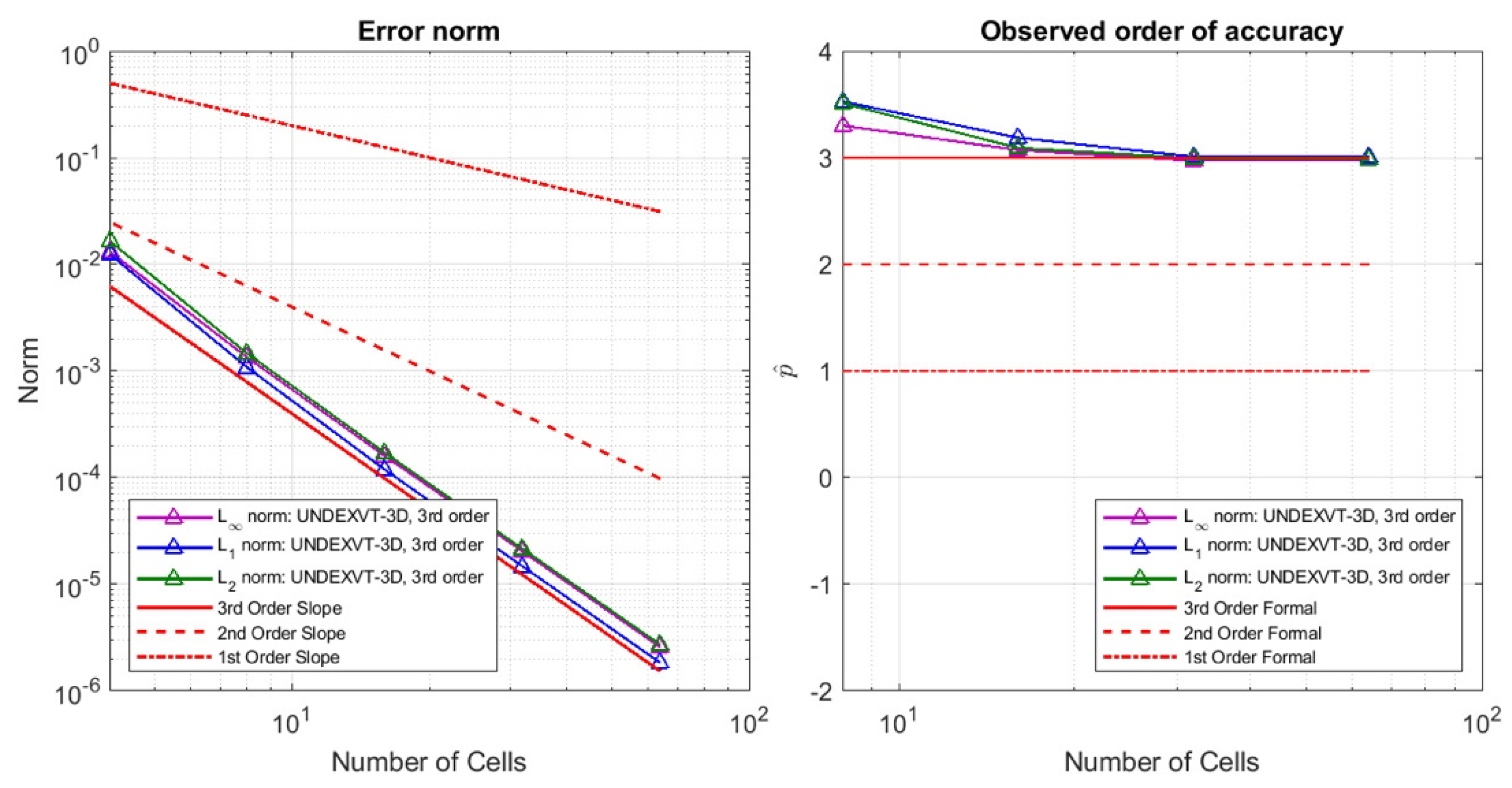
As an example, the error norms and the observed order of accuracy tested on the 3D third-order solver are plotted in Figure 3. The numeric values are listed in Table 3.

Figure 3. Observed order of accuracy of the 3D third-order solver (left: error norm; right: observed order of accuracy).

Table 3. Observed order of accuracy of 3D third-order solver.

No. Cells	dx (= dy = dz)	No. Time Steps	dt	Observed Order of Accuracy
				${\mathbf{L}}_{\mathbf{\infty }} \mathbf{Norm}$	${\mathbf{L}}_1 \mathbf{Norm}$	${\mathbf{L}}_2 \mathbf{Norm}$
$4\times 4\times 4$	0.5	313	$3.2\times {10}^{-3}$	N/A	N/A	N/A
$8\times 8\times 8$	0.25	625	$1.6\times {10}^{-3}$	3.3012	3.5270	3.5101
$16\times 16\times 16$	0.125	1250	$8.0\times {10}^{-4}$	3.0714	3.1871	3.0921
$32\times 32\times 32$	0.0625	2520	$4.0\times {10}^{-4}$	2.9722	3.0099	2.9945
$64\times 64\times 64$	0.03125	5000	$2.0\times {10}^{-4}$	2.9839	3.0061	2.9832

Figure 3 and Table 3 indicate that the observed order of accuracy tested on the 3D third-order solver matches well with the formal order of accuracy. The 3D third-order solver succeeded in the order of accuracy verification. The order of accuracy verification on the 3D second- and first-order solvers was also conducted. The 3D second- and first-order plots will be included in the author’s dissertation.

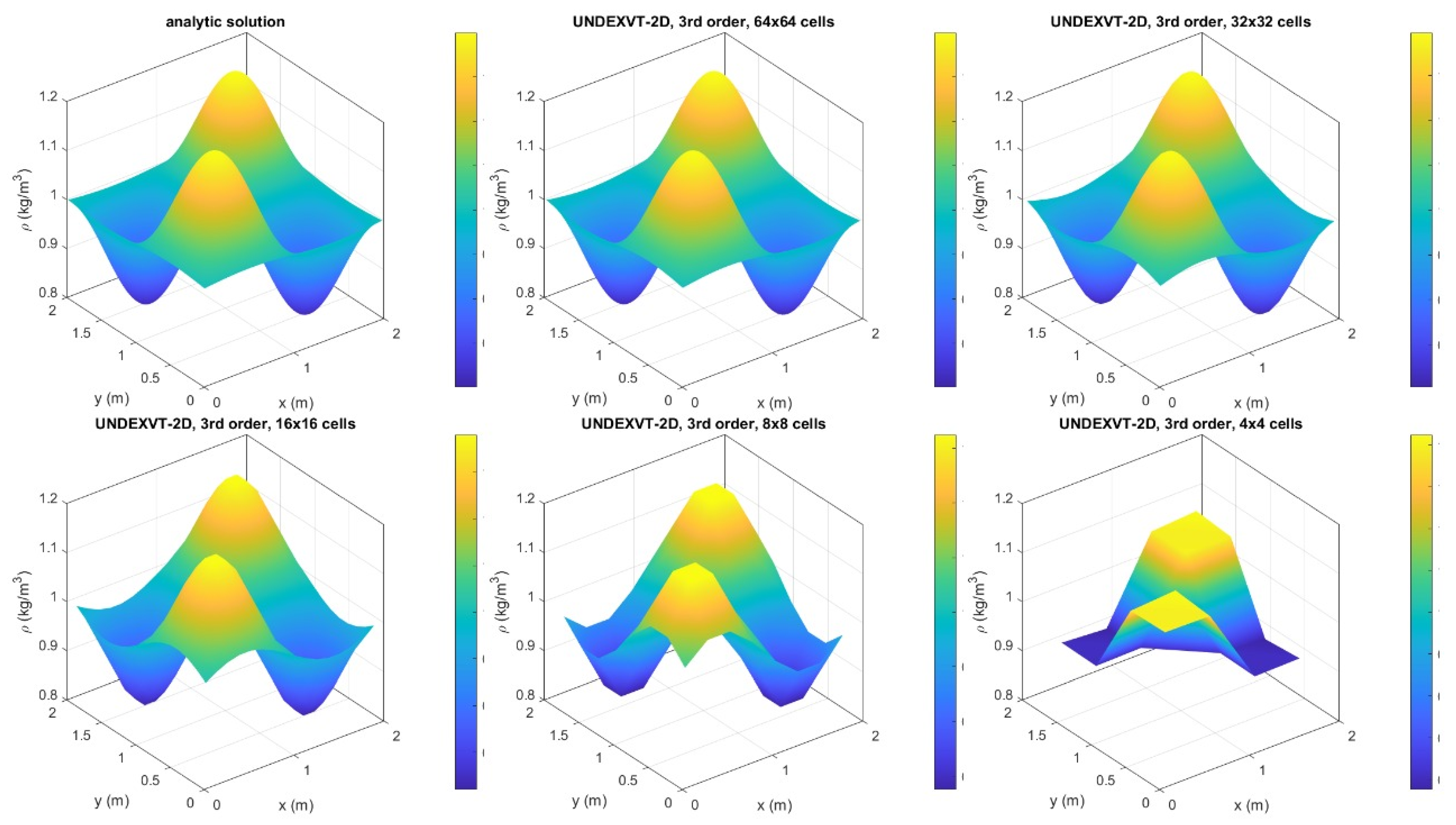
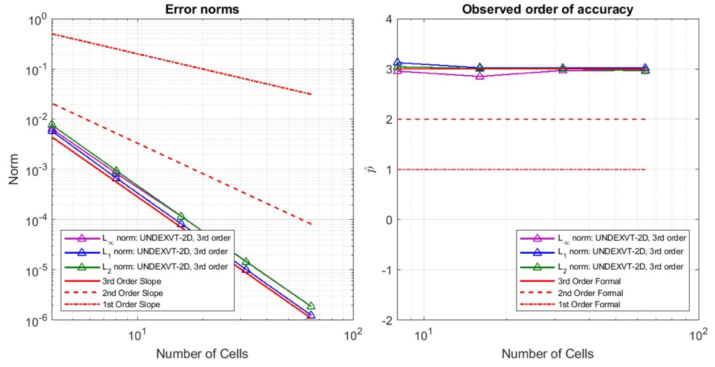
The order of accuracy verifications on 2D and 1D solvers are performed in a similar way. The simulation results using the 2D third-order solver performed on different grid levels are plotted in Figure 4. Their observed order of accuracy is plotted in Figure 5. The numeric values are listed in Table 4. Code verification on the second- and first-order solvers will be included in the author’s dissertation.

Figure 4. Simulation of the cases in Table 2 using a 2D third-order solver.

Figure 5. Observed order of accuracy of the 2D third-order solver (left: error norm; right: observed order of accuracy).

Table 4. Observed order of accuracy of the 2D third-order solver.

No. Cells	dx (= dy)	No. Time Steps	dt	Observed Order of Accuracy
				${\mathbf{L}}_{\mathbf{\infty }} \mathbf{Norm}$	${\mathbf{L}}_1 \mathbf{Norm}$	${\mathbf{L}}_2 \mathbf{Norm}$
$4\times 4$	0.5	313	$3.2\times {10}^{-3}$	N/A	N/A	N/A
$8\times 8$	0.25	625	$1.6\times {10}^{-3}$	2.9560	3.1252	3.0427
$16\times 16$	0.125	1250	$8.0\times {10}^{-4}$	2.8500	3.0225	3.0076
$32\times 32$	0.0625	2520	$4.0\times {10}^{-4}$	2.9699	3.0190	3.0062
$64\times 64$	0.03125	5000	$2.0\times {10}^{-4}$	2.9738	3.0184	2.9600

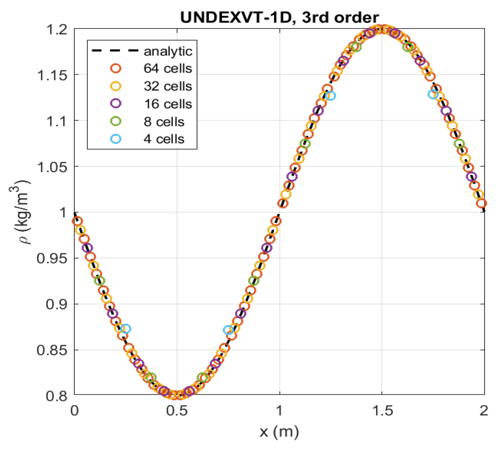
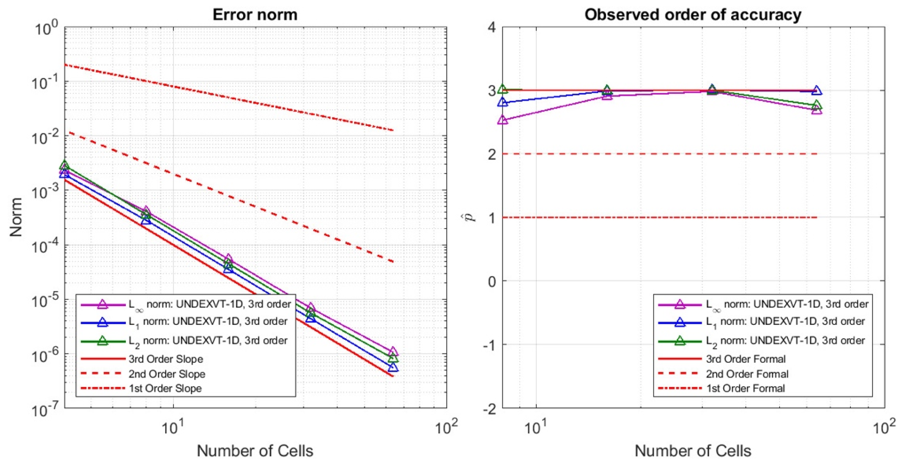
Figure 5 and Table 4 indicate that the observed order of accuracy for the 2D third-order solver matches the formal order of accuracy. The 2D third-order solver succeeded in the code verification. The simulation results using the 1D third-order solver performed on different grid levels are plotted in Figure 6. The observed order of accuracy is plotted in Figure 7. The numeric values are listed in Table 5.

Figure 6. Simulation of cases in the table using the 1D third-order solver.

Figure 7. Observed order of accuracy of the 1D third-order solver (left: error norm; right: observed order of accuracy).

Table 5. Observed order of accuracy of the 1D third-order solver.

No. Cells	dx	No. Time Steps	dt	Observed Order of Accuracy
				${\mathbf{L}}_{\mathbf{\infty }} \mathbf{Norm}$	${\mathbf{L}}_1 \mathbf{Norm}$	${\mathbf{L}}_2 \mathbf{Norm}$
$4$	0.5	313	$3.2\times {10}^{-3}$	N/A	N/A	N/A
$8$	0.25	625	$1.6\times {10}^{-3}$	2.5264	2.8016	3.0072
$16$	0.125	1250	$8.0\times {10}^{-4}$	2.9069	2.9881	2.9964
$32$	0.0625	2520	$4.0\times {10}^{-4}$	2.9801	3.0034	2.9982
$64$	0.03125	5000	$2.0\times {10}^{-4}$	2.6847	2.9799	2.7614

Figure 7 and Table 5 indicate that the observed order of accuracy for the 1D third-order solver matches the formal order of accuracy. The 1D third-order solver succeeded in the code verification.

4.2. Simulations of Single and Multi-Dimensional Configurations

The simulation of single and multi-dimensional configurations that reflect near-field and early-time UNDEX are performed using the UNDEXVT solvers after the code verifications are performed. These simulations are also compared with analytic solutions if they exist, experiments, and simulations using other algorithms conducted in previous research described in the literature. The cases to be simulated are summarized in Table 6.

Table 6. Cases to be simulated using the UNDEXVT solver.

Case #	Description	Notes
1	1D Riemann problem: multi-phase, single material	Comparison w/analytic solutions
2	1D Riemann problem: multi-phase, multi-material	Comparison w/analytic solutions
3	3D explosion problem	Symmetry exists. 2D axi-symmetrical & 1D spherical
4	Dynamics of explosive gas bubble	TNT charge. Validated by experiments
5	Dynamics of explosive gas bubble	TNT charge. Used to assist research on accuracy of NRBC
6	Dynamics of explosive gas bubble	TNT charge. Used to assist research on NRBC and its effect on simulation of explosive gas bubble

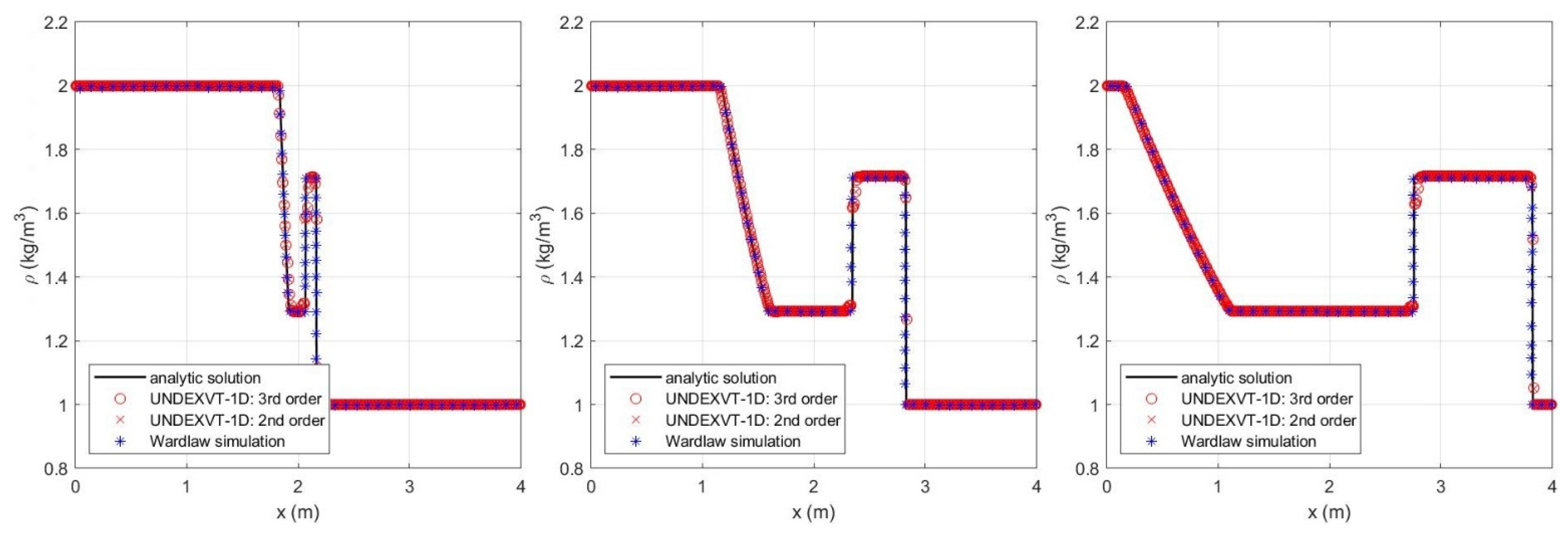
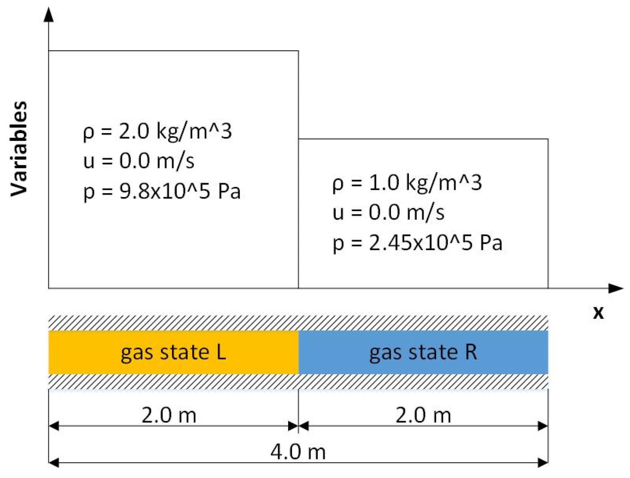
Case 1: In this case, a one-dimensional shock tube problem that consists of fluids of the same material is simulated using UNDEXVT-1D third- and second-order solvers. The configuration of this case is described as follows, and is illustrated in Figure 8. A domain of $\mathrm{x}\in \left[0.0,4.0\right]$ m is equally separated by fluids of states L and R in the initial condition. The density and pressure of fluid L are equal to $2.0 \mathrm{kg}/{\mathrm{m}}^3$ and $9.8\times {10}^5 \mathrm{Pa}$, respectively. The density and pressure of fluid R are equal to $1.0 \mathrm{kg}/{\mathrm{m}}^3$ and $2.45\times {10}^5 \mathrm{Pa}$, respectively. The velocities of both states equal zero in the initial condition.

Figure 8. ICs of Case 1.

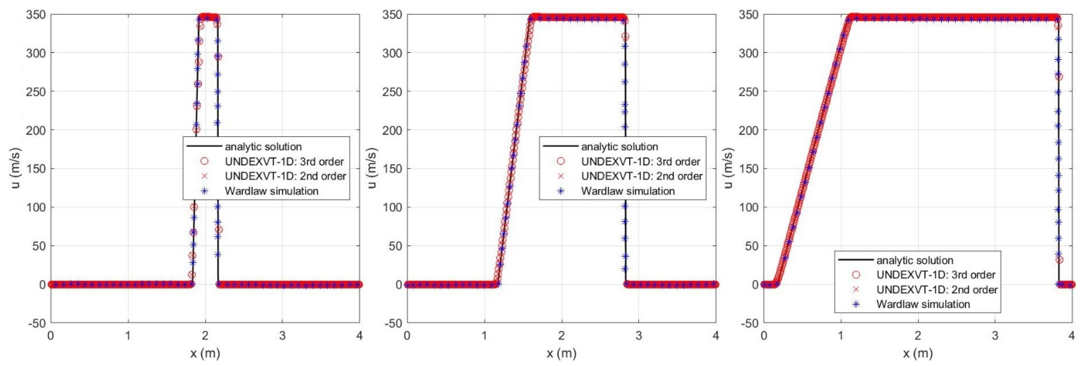
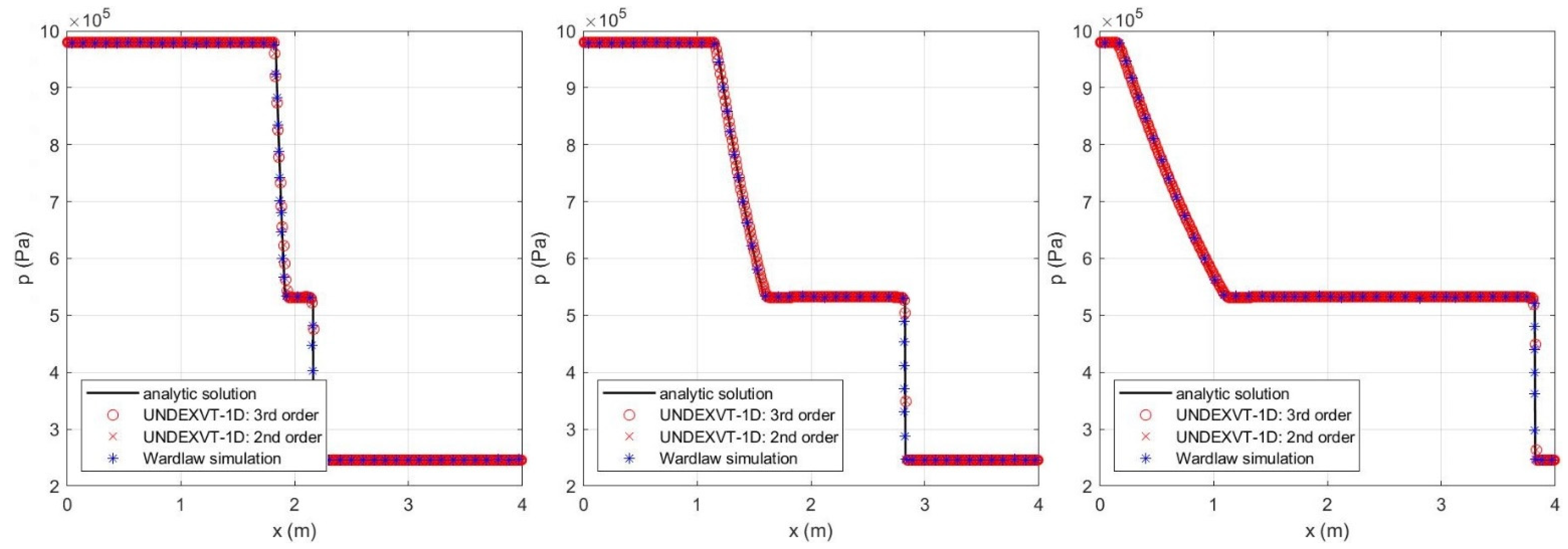
A Cartesian-structured mesh of 400 cells of uniform size is used to discretize the domain. The simulation is run up to $2.2\times {10}^{-3} \mathrm{s}$. Wardlaw performed a simulation of the same case, using numerical techniques of unknown types [41]. Solutions at $2.0\times {10}^{-4} \mathrm{s}$, $1.0\times {10}^{-3} \mathrm{s}$ and the final time are presented, along with analytic solutions and Wardlaw’s simulation solutions. The ideal gas equation of state is used to model the thermodynamic behavior of both fluids. The gas constant is equal to 1.4. The densities at these three times are plotted in Figure 9, the velocities are plotted in Figure 10, and the pressures are plotted in Figure 11.

Figure 9. Densities at $2.0\times {10}^{-4} \mathrm{s}$, $1.0\times {10}^{-3} \mathrm{s}$ and $2.2\times {10}^{-3} \mathrm{s}$ (from left to right).

Figure 10. Velocities at $2.0\times {10}^{-4} \mathrm{s}$, $1.0\times {10}^{-3} \mathrm{s}$ and $2.2\times {10}^{-3} \mathrm{s}$ (from left to right).

Figure 11. Pressures at $2.0\times {10}^{-4} \mathrm{s}$, $1.0\times {10}^{-3} \mathrm{s}$ and $2.2\times {10}^{-3} \mathrm{s}$ (from left to right).

These comparisons indicate that the simulations using the UNDEXVT-1D third-order and second-order solvers, Wardlaw simulation solutions and analytic solutions show excellent agreement.

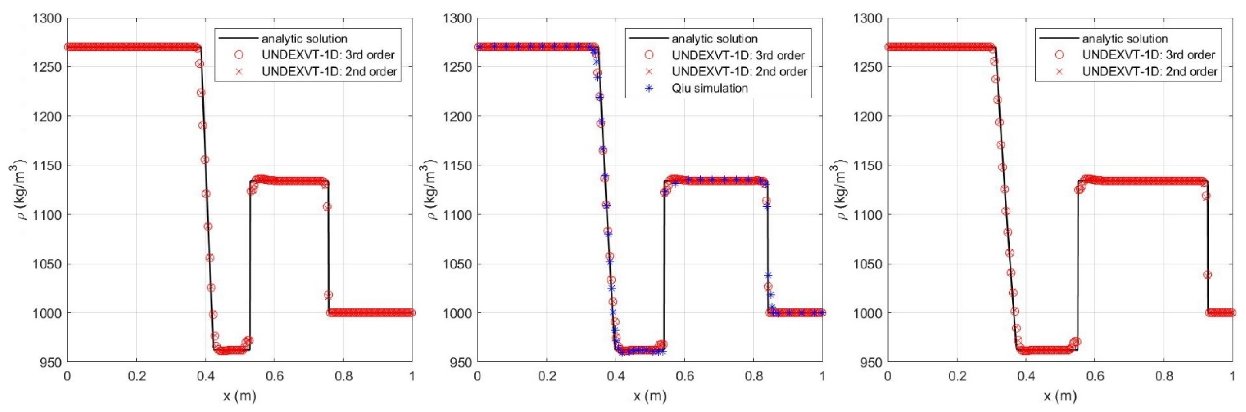
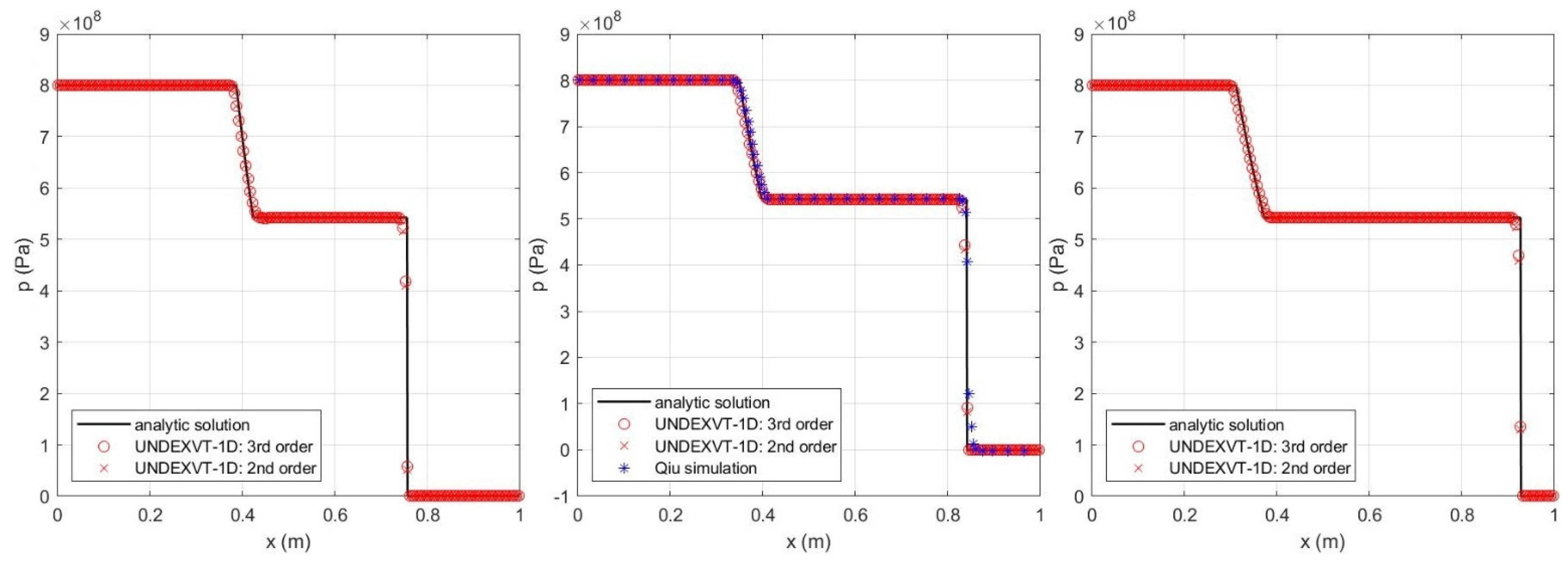
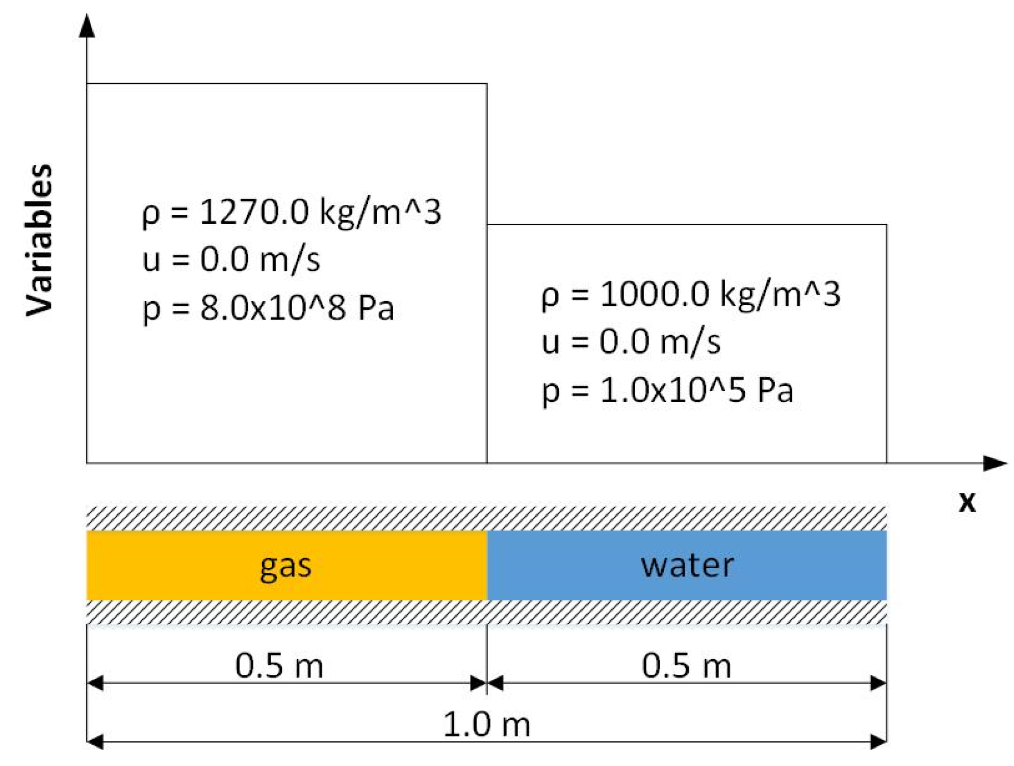
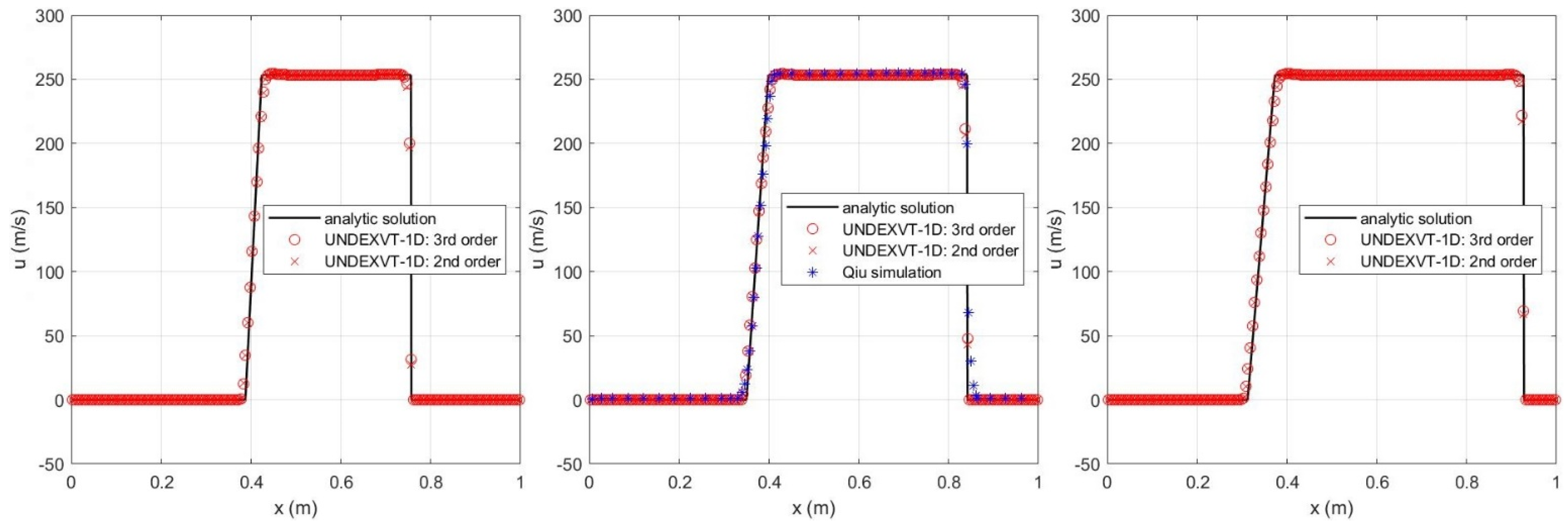
Case 2: In this case, a one dimensional shock tube problem that consists of fluids of different materials is simulated using UNDEXVT-1D third- and second-order solvers. The configuration of this case is illustrated in Figure 12, and is described as follows. A domain of $\mathrm{x}\in \left[0.0,1.0\right]$ m is equally separated by gas and water of different states in the initial condition. The density and pressure of the gas is equal to $1270.0 \mathrm{kg}/{\mathrm{m}}^3$ and $8.0\times {10}^8 \mathrm{Pa}$, respectively. The density and pressure of the water are equal to $1000.0 \mathrm{kg}/{\mathrm{m}}^3$ and $1.0\times {10}^5 \mathrm{Pa}$, respectively. The velocities of both states equal zero in the initial conditions.

Figure 12. ICs of Case 2.

A Cartesian-structured mesh of 200 cells of uniform size is used to discretize the domain. The simulation is run up to $2.0\times {10}^{-4} \mathrm{s}$. Qiu [42] performed a simulation of the same case, using the same fluid discretization algorithms but with the GFM modified by Liu [34,36]. The solutions at $1.2\times {10}^{-4} \mathrm{s}$, $1.6\times {10}^{-4} \mathrm{s}$ and the final time are presented, along with analytic solutions and Qiu’s simulation at $1.6\times {10}^{-4} \mathrm{s}$. The ideal gas equation of state is used to model the thermodynamic behavior of the gas. The gas constant is equal to 1.4. The stiffened equation of state is adopted to model the thermodynamic behavior of the water, and is expressed as

$$\mathrm{p}=\left({\mathsf{\gamma }}_{\mathrm{B}}-1\right){\mathsf{\rho }\mathrm{e}}^{\mathrm{int}}-{\mathsf{\gamma }}_{\mathrm{B}}\mathrm{B}$$

(23)

where ${\mathsf{\gamma }}_{\mathrm{B}}$ and $\mathrm{B}$ are the parameters for which the values are the same as in [42]. The densities at these three times are plotted in Figure 13, the velocities are plotted in Figure 14, and the pressures are plotted in Figure 15.

Figure 13. Densities at $1.2\times {10}^{-4} \mathrm{s}$, $1.6\times {10}^{-4} \mathrm{s}$ and $2.0\times {10}^{-4} \mathrm{s}$ (from left to right).

Figure 14. Velocities at $1.2\times {10}^{-4} \mathrm{s}$, $1.6\times {10}^{-4} \mathrm{s}$ and $2.0\times {10}^{-4} \mathrm{s}$ (from left to right).

Figure 15. Pressures at $1.2\times {10}^{-4} \mathrm{s}$,$1.6\times {10}^{-4} \mathrm{s}$ and $2.0\times {10}^{-4} \mathrm{s}$ (from left to right).

These comparisons indicate that the simulations using the UNDEXVT-1D third-order and second-order solvers, the simulations using Qiu’s algorithms, and the analytic solutions show excellent agreement.

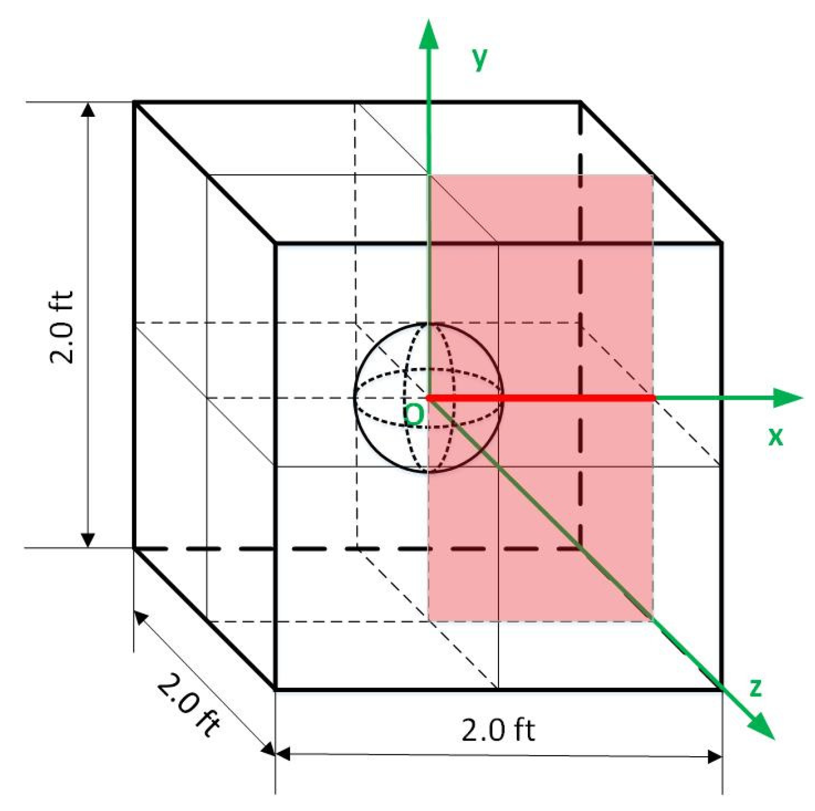
Case 3: In this case, a three-dimensional UNDEX problem is simulated using UNDEXVT-3D third- and second-order solvers. The explosive gas sphere, upon the completion of the ignition and chemical reaction, has a radius of 4.0 inches, and is in a rectangular domain of $\mathrm{x}\in \left[-1.0,1.0\right]$ ft, $\mathrm{y}\in \left[-1.0,1.0\right]$ ft and $\mathrm{z}\in \left[-1.0,1.0\right]$ ft at $\left(\mathrm{x},\mathrm{y},\mathrm{z}\right)=\left(0.0,0.0,0.0\right)$ ft. The gas is surrounded by liquid water. The density and pressure of the gas are equal to $1630.0 \mathrm{kg}/{\mathrm{m}}^3$ and $7.8039\times {10}^9 \mathrm{Pa}$, respectively. The density and pressure of the water are equal to $1000.0 \mathrm{kg}/{\mathrm{m}}^3$ and $1.0\times {10}^5 \mathrm{Pa}$, respectively. The velocities of both equal zero in the initial condition. This configuration is illustrated in Figure 16.

Figure 16. ICs of Case 3.

A Cartesian-structured mesh of $200\times 200\times 200$ cells of uniform size is used to discretize the domain. The simulation is run for $4.55\times {10}^{-5} \mathrm{s}$. Cooke et al. performed a simulation in the same case using a sub-cell resolution scheme with the front tracking method proposed by them [43]. The ideal gas equation of state is used to model the thermodynamic behavior of the gas with the same gas constant used in Cases 1 and 2. The Tait equation of state is used to model the thermodynamic behavior of the water, and is expressed as

$$\mathrm{p}=\mathrm{B}\left[{\left(\frac{\mathsf{\rho }}{{\mathsf{\rho }}_0}\right)}^{\mathrm{N}}-1\right]+\mathrm{A}$$

(24)

where $\mathrm{N}$, $\mathrm{B}$ and $\mathrm{A}$ are the parameters for which the values are the same as in [5]. Because of the symmetry in this configuration and because the characteristic wave, i.e., the shock wave, does not arrive at the boundary within the time range of the simulation, 2D axi-symmetric and 1D spherical simulations can also be performed, as shown in Figure 16. The discretization of the 3D and 2D axi-symmetric domain is shown in Figure 17 using the density initial conditions for illustration. In total, 1/8 of the 3D domain is plotted, but the full domain is used for the computation.

Figure 17. Discretization of 3D and 2D axi-symmetric domains and the gaseous bubble.

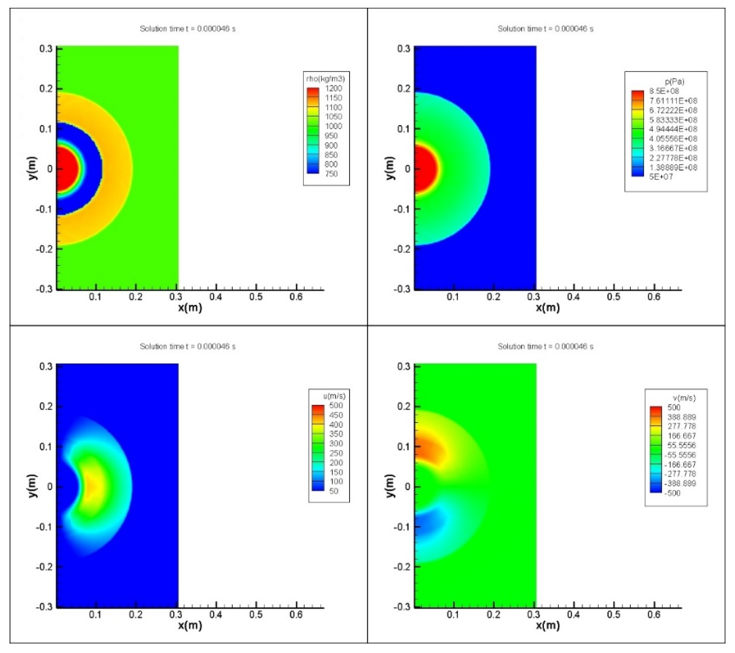
Contours including the primitive variables at $4.55\times {10}^{-5} \mathrm{s}$ using the 3D third-order solver are plotted in Figure 18. In total, 1/8 of the domain is plotted, but the full domain is used for the computation. Contours using the 2D axi-symmetric third-order solver are plotted in Figure 19. The comparisons between the 3D, 2D axi-symmetric and 1D spherical simulations using both the third and second-order solvers are shown by plotting the density, velocity in the x direction, and pressure along the 1D domain of $\mathrm{x}\in \left[-1.0,1.0\right]$ ft, $\mathrm{y}=0.0$ ft and $\mathrm{z}=0.0$ ft, and are shown in Figure 20.

Figure 18. Solution at $4.55\times {10}^{-5} \mathrm{s}$ using a 3D third-order solver (top left: density; top right: pressure; bottom: velocities in the x, y and z directions from left to right).

Figure 19. Solution at $4.55\times {10}^{-5} \mathrm{s}$ using a 2D axi-symmetric third-order solver (top left: density; top right: pressure; bottom: velocities in the x and y directions from left to right).

Figure 20. Comparison of the simulations using 3D, 2D axi-symmetric and 1D spherical solvers (left column: simulation using second-order solvers; right column: simulation using third-order solvers; from top to bottom: density, velocity in the x direction, and pressure).

Figure 20 indicates that the 3D, 2D axi-symmetric and 1D spherical simulations show good agreement. Because of this, the simulation using a lower degree and order can be used if symmetry exists in the configuration of the UNDEX case.

4.3. Simulation of the Bubble Dynamics and the Application of Non-Reflecting Boundary Conditions

When an underwater explosion occurs, the explosive gas bubble expands because its pressure significantly exceeds that of the surrounding water. Then, the pressure decays as the gas bubble overshoots and continues to grow in size. The bubble keeps growing in size beyond the moment when its pressure is balanced by that of the surrounding water because of its inertia. It keeps expanding, but at a decreasing rate, and eventually stops. After this, the explosive gas bubble contracts because the pressure of the water now exceeds the gas pressure. During the contraction, a pressure balance is reached again between the gas and water, but the gas bubble continues to contract due to inertia, and eventually stops. This cycle of expanding and contracting continues to occur. The maximums of the bubble radius decrease while the minimums of the bubble radius increase because energy keeps dissipating [1]. The UNDEXVT CFD solver can conduct the simulation of bubble dynamics in underwater explosions, although this was not its intended purpose. As an example, Case 4 simulates the variation of the radius of an explosive gas bubble over time, as validated by experiments.

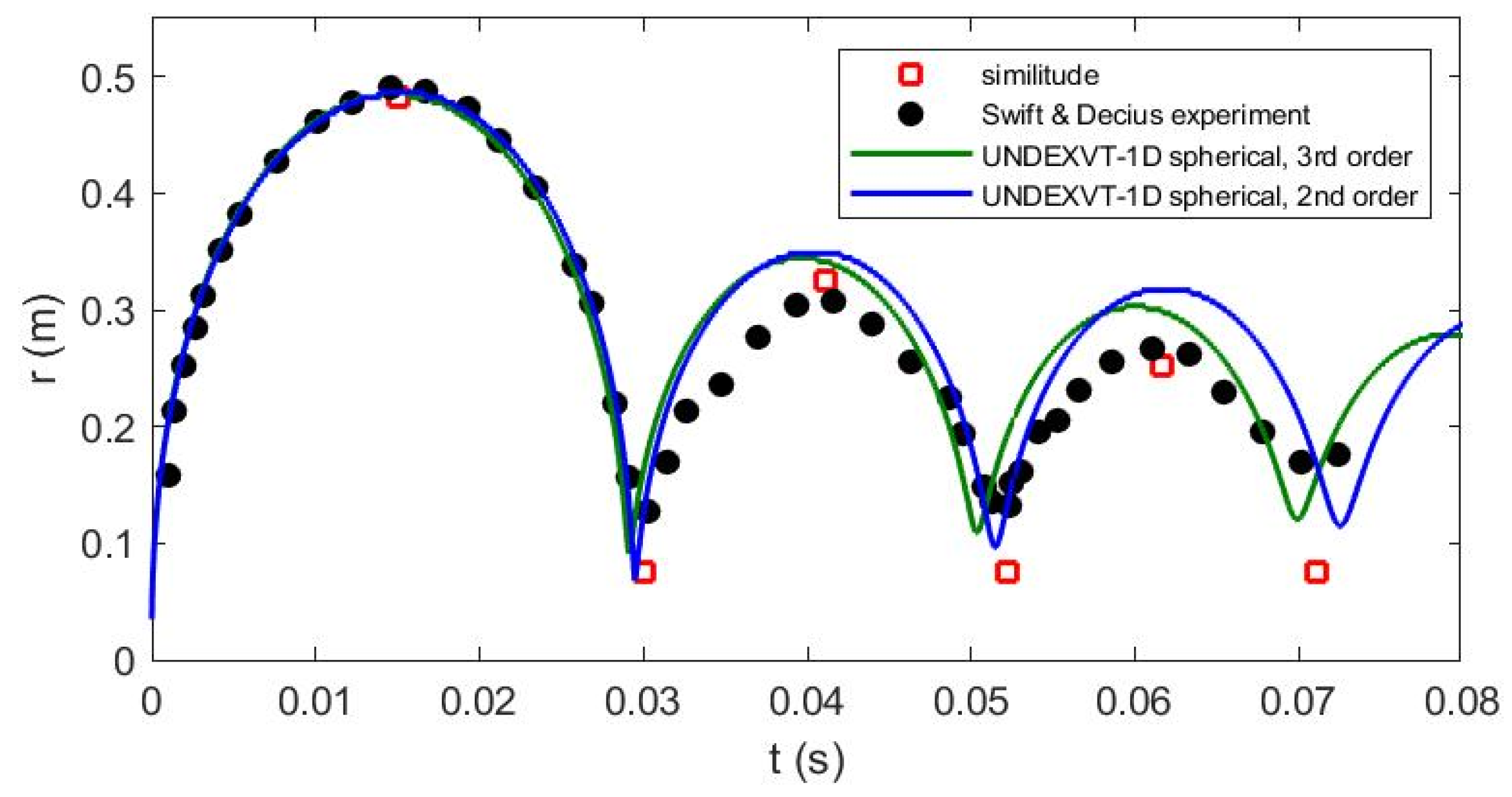
Case 4: This case considers a 0.66 lb TNT charge exploding at 300 ft and 550 ft below the surface, respectively. Because the charge is immersed deeply, the effect of gravity, the linear variation of the hydrostatic water pressure and the free surface is neglected. The configuration is considered to be symmetric about the charge center. A 1D spherical simulation is used to take advantage of this symmetry. This experiment was performed by Swift and Decius [44], and the results were reproduced by simulation using the UNDEXVT solvers. The JWL equation of state is applied to model the explosive gas with the TNT parameters specified in [45]. The Tait equation of state is applied to model the surrounding water, with the water parameters specified in [5]. The initial conditions of both states are determined. The simulation is first run up to 0.035 s. The variation of the bubble radius with the first bubble period is plotted and compared with the Swift and Decius [44] experiments and the Aron and Cole similitude equations [1,11] in Figure 21.

Figure 21. Variation of the bubble radius over time, for 0.66 lb TNT exploding 300 ft and 550 ft below the surface (from left to right).

The experimental results of multiple bubble periods for the 300 ft case are also provided by [44]. The UNDEXVT simulation is run up to a later time of 0.08 s to capture multiple bubble periods, and the results are compared with the experimental and similitude equation results, as shown in Figure 22.

Figure 22. Variation of the bubble radius over time, for 0.66 lb TNT exploding 300 ft below the surface, for multiple bubble periods.

Figure 21 and Figure 22 indicate that the simulation using the UNDEXVT solvers matches well with the experiments in the first bubble period. In subsequent bubble periods, the simulations over-predicts the maximums and minimums of the bubble radius, suggesting that the simulation is not predicting all of the energy loss in later time. This is likely because there are energy-dissipating mechanisms not being considered in the simulation, for example the viscosity and turbulence in the fluid. The simulation does successfully predict the timing of the bubble maximums and minimums in the first and subsequent bubble periods. Because the early-time response is most important in our study, this is considered sufficient.

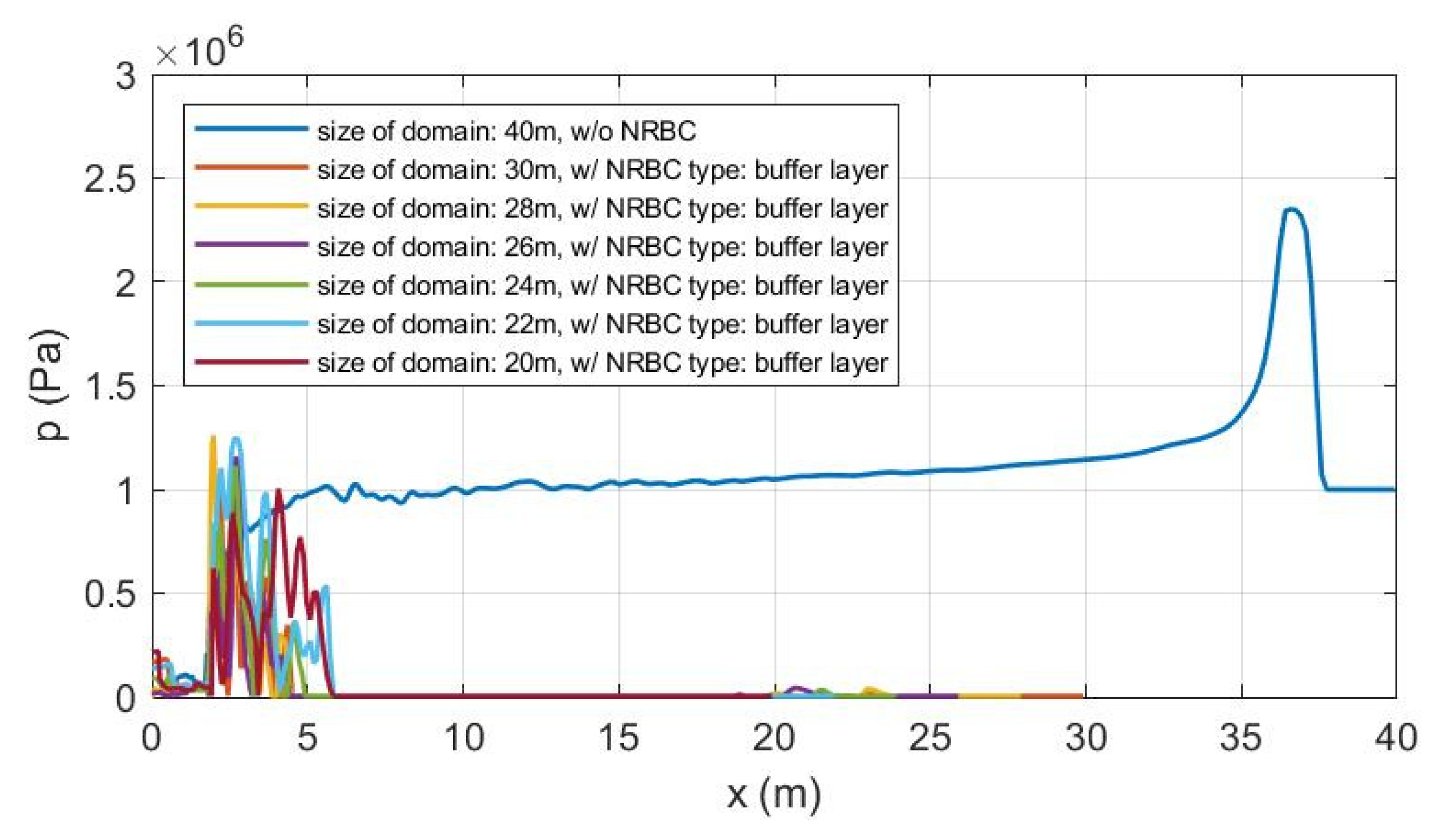
Case 5: In Case 4, the computational domain is set large enough that the characteristic shock wave does not reach the boundary within the total time of the simulation. Because of this, in a hyperbolic problem, the boundary condition has no influence on the solution. However, in order to save computing resources, especially memory, and to make the simulation more efficient, the domain cannot be too large. This is particularly true if the simulation is required to last until a late time, such that the wave travels very far. The effective implementation of the best possible non-reflecting boundary condition is therefore essential in the simulation. The literature indicates that the implementation of NRBCs is still a developing science, in that there is currently no perfect way to impose this type of boundary condition. This is especially true for a discontinuous shock wave. The objective in this research is to identify the best available NRBC choice for absorbing shock waves consistent with our hybrid framework of algorithms. Four different NRBCs are introduced and compared. Three of them are from the literature, and the last was devised by the author. A simple test case is used to assess the performance of these NRBCs in terms of their ability to absorb the wave and keep it from reflecting. In this case, a 28 kg TNT charge is exploded 178 m below the surface. A 1D spherical simulation is conducted to predict the flow, as in Case 4. Initial conditions are determined based on the parameters of the equation of state provided by [5,45]. In order to investigate the performance of the NRBCs, a simulation using a very large domain without NRBC is run long enough that the characteristic wave falls just short of reaching the boundary. Then, the simulations are run using domains of limited size with the different NRBCs, such that an NRBC is needed to absorb the wave.

In the first NRBC case, a buffer layer is created on the boundary, discretized like the fluid domain. An extra source term is added to the right-hand side of the governing equations, Equation (1). The extra source term is zero, however, in all of the cells other than the buffer layer at the boundary of the fluid domain. Using the two-dimensional configuration as an example, the buffer layer is added at the boundary of the fluid domain. The source term that is non-zero in the buffer zone is

$${\overrightarrow{\mathrm{S}}}_{\mathrm{BC}}=-\mathsf{\sigma }\left(\mathrm{x},\mathrm{y}\right)\left\{\mathsf{\rho },\mathsf{\rho }\mathrm{u},\mathsf{\rho }\mathrm{v},\mathsf{\rho }\mathrm{E}\right\}$$

(25)

where

$\mathsf{\sigma }={\mathsf{\sigma }}_{\mathrm{x}}+{\mathsf{\sigma }}_{\mathrm{y}}$,

${\mathsf{\sigma }}_{\mathrm{x}}=\mathrm{a}{\left[\frac{\mathrm{x}-{\mathrm{x}}_{\mathrm{L}1}}{{\mathrm{W}}_{\mathrm{L}}}\right]}^{\mathrm{n}}$ for ${\mathrm{x}}_{\mathrm{L}2}\le \mathrm{x}\le {\mathrm{x}}_{\mathrm{L}1}$, and

${\mathsf{\sigma }}_{\mathrm{y}}=\mathrm{a}{\left[\frac{\mathrm{y}-{\mathrm{y}}_{\mathrm{B}1}}{{\mathrm{W}}_{\mathrm{B}}}\right]}^{\mathrm{n}}$ for ${\mathrm{y}}_{\mathrm{B}2}\le \mathrm{y}\le {\mathrm{y}}_{\mathrm{B}1}$. Refer to references [46,47,48] for more details. The performance of this buffer layer NRBC is illustrated in Figure 23.

Figure 23. Buffer layer type NRBC and its performance.

Figure 23 shows that this close-in NRBC is not able to absorb the shock wave. It also reflects noise back to the fluid domain, such that the distribution of pressure becomes chaotic. Research performed by [46] also suggests that the buffer layer type of NRBC will be unsuccessful if the governing equations have nonlinear terms, unless extra stability adjustments are made. The damping region, i.e., the buffer layer, also needs to be quite large [46].

Next, a free outflow type of NRBC is imposed at the boundary of the fluid domain [5,48]. The implementation of a free outflow type of NRBC is straightforward. Specifically, it requires that gradients of conservative variables (or primitive variables) with respect to the outward normal direction at the boundary face equal zero. In the discretization level, one can enforce a zero-order extrapolation. Refer to references [5,48] for more details. Ideally, there should be no reflection. Its performance is illustrated in Figure 24.

Figure 24. Free outflow type of NRBC, and its performance.

Figure 24 indicates that the free outflow type of NRBC outperforms the buffer layer in that it successfully absorbs the shock wave and does not reflect it, but the size of the domain affects the solution accuracy with any significant domain size reduction, meaning that it is of limited value.

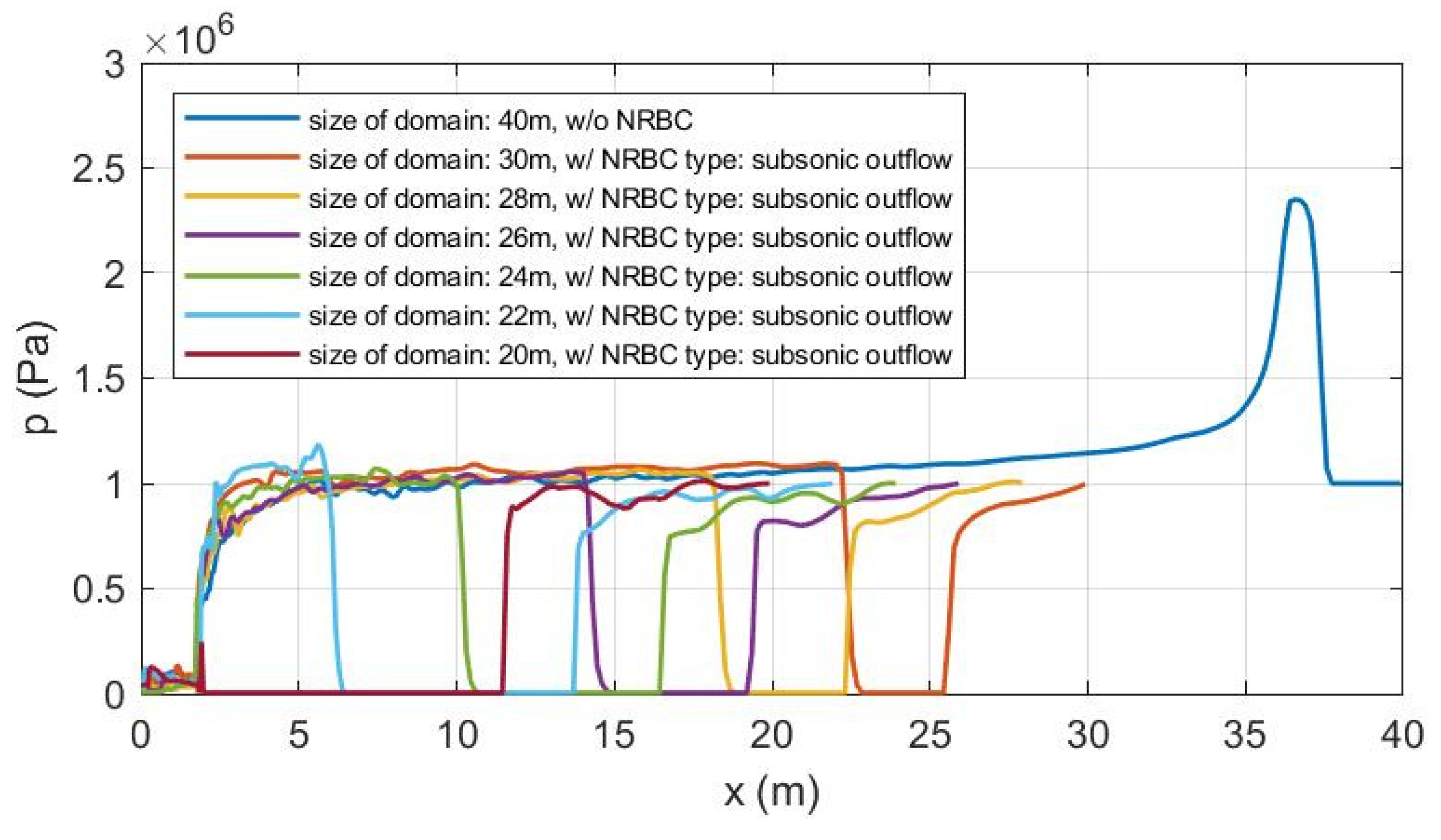
The third type of NRBC is the subsonic outflow condition. The mathematical derivation of this subsonic outflow condition involves a compressible CFD characteristic analysis. The implementation of this type of NRBC is also more complicated than in the previous two types. A cell stencil at the boundary is illustrated in Figure 25. In this diagram, d denotes a boundary cell, b denotes a boundary, and g denotes a ghost cell. The details of its implementation are described in Equation (26).

$$\{\begin{array}{c}{\mathrm{p}}_{\mathrm{b}}={\mathrm{p}}_{\infty }\\ {\mathrm{c}}_{\mathrm{b}}={\mathrm{c}}_{\mathrm{d}}\\ {\mathsf{\rho }}_{\mathrm{b}}={\mathsf{\rho }}_{\mathrm{d}}+\left({\mathrm{p}}_{\mathrm{b}}-{\mathrm{p}}_{\mathrm{d}}\right)/{\mathrm{c}}_{\mathrm{b}}^2\\ {\overrightarrow{\mathrm{v}}}_{\mathrm{b}}={\overrightarrow{\mathrm{v}}}_{\mathrm{d}}+\hat{\mathrm{n}}\left({\mathrm{p}}_{\mathrm{d}}-{\mathrm{p}}_{\mathrm{b}}\right)/\left({\mathsf{\rho }}_{\mathrm{b}}{\mathrm{c}}_{\mathrm{b}}\right)\end{array}$$

(26)

and then ${\overrightarrow{\mathrm{U}}}_{\mathrm{g}}=2{\overrightarrow{\mathrm{U}}}_{\mathrm{b}}-{\overrightarrow{\mathrm{U}}}_{\mathrm{d}}$ where $\overrightarrow{\mathrm{U}}={\left\{\mathsf{\rho },\mathsf{\rho }\mathrm{u},\mathsf{\rho }\mathrm{v},\mathsf{\rho }\mathrm{w},\mathsf{\rho }\mathrm{E}\right\}}^{\mathrm{T}}$.

Figure 25. Cell stencil at the boundary.

Refer to references [49,50] for more details. The performance for this NRBC is shown in Figure 26.

Figure 26. Subsonic outflow type of NRBC, and its performance.

Figure 26 shows that this NRBC absorbs the shock wave without reflecting chaotic noise, and the accuracy of this type of NRBC is not affected by the domain size; however, it reflects a cavitation zone back into the fluid, which substantially distorts the flow solution.

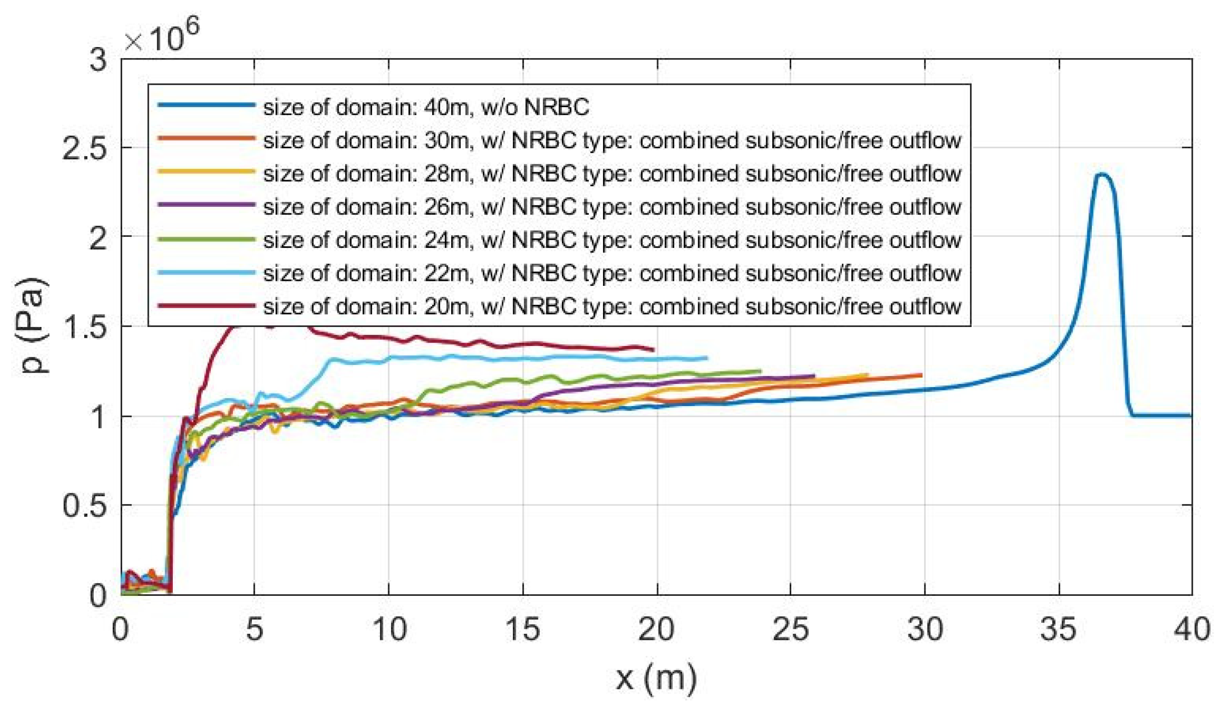
A mixed free/subsonic outflow type of NRBC was eventually devised. In this mixed free/subsonic outflow type of NRBC, the subsonic outflow condition is applied to the pressure, while the free outflow condition is applied to the rest of the primitive variables. A cell stencil at the boundary for this NRBC is illustrated in Figure 25. In this diagram, d denotes a boundary cell, b denotes a boundary, and g denotes a ghost cell. The details of its implementation are described in Equation (27). Its performance is shown in Figure 27.

$$\{\begin{array}{c}{\mathsf{\rho }}_{\mathrm{b}}={\mathsf{\rho }}_{\mathrm{d}}\\ {\overrightarrow{\mathrm{v}}}_{\mathrm{b}}={\overrightarrow{\mathrm{v}}}_{\mathrm{d}}\\ {\mathrm{c}}_{\mathrm{b}}={\mathrm{c}}_{\mathrm{d}}\\ {\mathrm{p}}_{\mathrm{b}}={\mathrm{p}}_{\infty }+{\mathsf{\rho }}_{\mathrm{b}}{\mathrm{c}}_{\mathrm{b}}{\overrightarrow{\mathrm{v}}}_{\mathrm{b}}·\hat{\mathrm{n}}\end{array}$$

(27)

and then ${\overrightarrow{\mathrm{U}}}_{\mathrm{g}}=2{\overrightarrow{\mathrm{U}}}_{\mathrm{b}}-{\overrightarrow{\mathrm{U}}}_{\mathrm{d}}$ where $\overrightarrow{\mathrm{U}}={\left\{\mathsf{\rho },\mathsf{\rho }\mathrm{u},\mathsf{\rho }\mathrm{v},\mathsf{\rho }\mathrm{w},\mathsf{\rho }\mathrm{E}\right\}}^{\mathrm{T}}$.

Figure 27. Mixed free/subsonic outflow type of NRBC, and its performance.

Figure 27 indicates that the mixed free/subsonic outflow type of NRBC is able to absorb the shock wave, and it does not reflect a cavitation zone back. The size of the domain also has less effect on the accuracy, and will allow substantial domain reduction.

Case 6: Next, an explosive charge of 227 kg TNT at 45 m below the surface is investigated. References [51,52] provide the numerical results for comparison with this case. This case is used to further explore the performance of non-reflecting boundary conditions and their application to the simulation of bubble dynamics where the simulation time is relatively long and there are multiple bubble periods in the time history. A simulation using a large domain is first performed without an NRBC, such that the shock wave does not reach the boundary within the simulation time. Simulations using domains of limited size are then performed, such that an NRBC is needed. The accuracy for the four types of NRBC is compared in Figure 28.

Figure 28. Comparison of the accuracy of the NRBCs.

Figure 28 shows that the buffer layer and free outflow types of NRBCs do not function well, and cause a run-time error. The subsonic outflow and the mixed free/subsonic outflow types of NRBCs are both successful in this case, but the time history of the bubble radius produced using the subsonic outflow type of NRBC becomes unsmooth during the contracting phase of the second bubble pulse, likely due to the interaction between the fluid domain and the cavitation zone reflected from the boundary.

4.4. Embedded Boundary Method and the Simulation of the Fluid–Structure Interaction

Instead of using a dynamic mesh method such as the arbitrary Laganrian–Eulerian method, this fluid solver uses an embedded boundary method, such that the fluid domain does not need to be body-conforming. A rectangular fluid domain is built and discretized using a Cartesian-structured mesh. Another advantage of a structured mesh over an unstructured mesh is that it helps stabilize the schemes and thus the simulation. Furthermore, the mesh is fixed even if the fluid domain is deforming.

The embedded boundary method consists of two parts: the accurate tracking of the geometry of the embedded wetted surface, and the imposition of the slip-wall boundary conditions. Necessary adjustments are made to the existing geometry-tracking scheme, such that a special topological issue is successfully solved, and thus the applicability of this scheme is extended. More details along with the UNDEX FSI simulations will be presented in a future paper.

5. Conclusions

This paper summarizes the development of a CFD solver based on a hybrid framework of algorithms for the simulation of near-field and early-time underwater explosions (UNDEX). The solver developed based on this framework of algorithms possesses reasonable computational efficiency, and is intended for the purpose of early-stage ship design. These algorithms include the Runge–Kutta method, the discontinuous Galerkin method, the level set method, the direct ghost fluid method, and the embedded boundary method.

A unique derivation with a multi-dimensional discretization on a Cartesian-structured mesh of the advection-dominated governing equations using Legendre polynomials selected in the manner of a Pascal triangle was introduced. Order of accuracy verifications were performed after the CFD solvers were developed. UNDEX cases of single and multi-dimensional configurations were simulated. Comparisons were made among the simulations using the developed solvers, simulations using other algorithms, and analytic solutions. The dynamics of explosive bubbles in UNDEX were also simulated and validated by experiments. A satisfying match between the experiments and simulations was observed. The selection of a non-reflecting boundary condition was achieved by comparing the behavior of a shockwave incident on a boundary and the behavior when applied in and UNDEX bubble simulation. Research applying this framework with the embedded boundary method in an FSI simulation for near-field UNDEX and more details on the formulation and application of a direct ghost fluid method (DGFM) will be the focus of future papers.

References

Cole, R.H. Underwater Explosion; Princeton University Press: Princeton, NJ, USA, 1948. [Google Scholar]
Klenow, B. Finite and Spectral Element Methods for Modeling Far-Field Underwater Explosion Effects on Ships Finite and Spectral Element Methods for Modeling Far-Field Underwater Explosion Effects on Ships; Virginia Tech: Blacksburg, VA, USA, 2009. [Google Scholar]
Klenow, B. Assessment of LS-DYNA and Underwater Shock Analysis (USA) Tools for Modeling Far-Field Underwater Explosion Effects on Ships Master of Science in Ocean Engineering; Virginia Tech: Blacksburg, VA, USA, 2006. [Google Scholar]
Keil, A.H. The Response of Ships to Underwater Explosions; David Taylor Model Basin: Bethesta, MD, USA, 1961. [Google Scholar]
Park, J. A Coupled Runge Kutta Discontinuous Galerkin-Direct Ghost Fluid (RKDG-DGF ) Method to Near-Field Early-Time Underwater Explosion ( UNDEX ) Simulations; Virginia Tech: Blacksburg, VA, USA, 2008. [Google Scholar]
Lu, Z.; Brown, A. Application of the Spectral Element Method in a Surface Ship Far-Field UNDEX Problem. Shock Vib.2019. [Google Scholar] [CrossRef] [Green Version]
Lu, Z.; Brown, A.J. Assessment of a new mesh generation and modeling approach for the surface ship far-field underwater explosion problem. In SNAME Maritime Convention; OnePetro: Richardson, TX, USA, 2019. [Google Scholar]
Klaseboer, E.; Hung, K.C.; Wang, C.; Wang, C.W.; Khoo, B.C.; Boyce, P.; Debono, S.; Charlier, H. Experimental and numerical investigation of the dynamics of an underwater explosion bubble near a resilient/rigid structure. J. Fluid Mech.2005, 537, 387–413. [Google Scholar] [CrossRef]
Lord Rayleigh, O.M.F.R.S. VIII. On the pressure developed in a liquid during the collapse of a spherical cavity, London, Edinburgh. Dublin Philos. Mag. J. Sci.1917, 34, 94–98. [Google Scholar] [CrossRef]
Plesset, M.S. The Dynamics of Cavitation Bubbles. J. Appl. Mech.1949, 16, 277–282. [Google Scholar] [CrossRef]
Arons, A.B. Secondary Pressure Pulses Due to Gas Globe Oscillation in Underwater Explosions. II. Selection of Adiabatic Parameters in the Theory of Oscillation. J. Acoust. Soc. Am.1948, 20, 277–282. [Google Scholar] [CrossRef]
Rohde, A. Eigenvalues and eigenvectors of the euler equations in general geometries. In Proceedings of the 15th AIAA Computational Fluid Dynamics Conference, Anaheim, CA, USA, 11–14 June 2001; pp. 1–6. [Google Scholar] [CrossRef] [Green Version]
Klenow, B.; Brown, A. Assessment of Non-Reflecting Boundary Conditions for Application in Far-Field UNDEX Finite Element Models. In Proceedings of the 77th Shock and Vibration Symposium, Monterrey, CA, USA, 29 October–2 November 2006; Available online: http://www.dept.aoe.vt.edu/~brown/Papers/NRBCSAVIAC2007.pdf (accessed on 15 November 2021).
Belytschko, T.; Liu, W.K.; Moran, B. Nonlinear Finite Elements for Continua and Structures; John Wiley & Sons: Hoboken, NJ, USA, 2000. [Google Scholar]
Wang, K.G. A Computational Framework Based on an Embedded Boundary Method for Nonlinear Multiphase Fluid Structure Interactions; Standford University: Stanford, CA, USA, 2011. [Google Scholar]
Si, N.; Park, J.; Brown, A.J. A Direct Ghost Fluid Method (DGFM) for Modeling Explosive Gas and Water Flows. J. Mar. Sci. Eng.2021. under review. [Google Scholar]
Flores, J.; Holt, M. Glimm’s Method Applied to Underwater Explosions. J. Comput. Phys.1981, 387, 377–387. [Google Scholar] [CrossRef]
Cocchi, J.P.; Saurel, R.; Loraud, J.C. Treatment of interface problems with Godunov-type schemes. Waves1996, 5, 347–357. [Google Scholar] [CrossRef]
Toro, E.F. Riemann Solvers and Numerical Methods for Fluid Dynamics, 3rd ed.; Springer: Berlin/Heidelberg, Germany, 2009. [Google Scholar]
Geuzaine, P.; Brown, G.; Harris, C.; Farhat, C. Aeroelastic dynamic analysis of a full F-16 configuration for various flight conditions. AIAA J.2003, 41, 363–371. [Google Scholar] [CrossRef]
Farhat, C.; Geuzaine, P.; Brown, G. Application of a three-field nonlinear fluid-structure formulation to the prediction of the aeroelastic parameters of an F-16 fighter. Comput. Fluids2003, 32, 3–29. [Google Scholar] [CrossRef]
Farhat, C.; Avery, P.; Tezaur, R.; Li, J. FETI-DPH: A dual-primal domain decomposition method for acoustic scattering. J. Comput. Acoust.2005, 13, 499–524. [Google Scholar] [CrossRef]
Avery, P.; Farhat, C.; Hetmaniuk, U. A Padé-based factorization-free algorithm for identifying the eigenvalues missed by a generalized symmetric eigensolver. Int. J. Numer. Methods Eng.2009, 79, 239–252. [Google Scholar] [CrossRef] [Green Version]
Miller, S.T.; Jasak, H.; Boger, D.A.; Paterson, E.G.; Nedungadi, A. A pressure-based compressible two-phase flow finite volume method for underwater explosions. Comput. Fluids2012, 87, 132–143. [Google Scholar] [CrossRef]
Reed, T.R.; Hill, W.H. Triangular Mesh Methods for Neutron Transport Equation; Los Alamos Scientific Laboratory: Ann Arbor, MI, USA, 1977. [CrossRef]
Cockburn, B. An introduction to the Discontinuous Galerkin method for convection-dominated problems. In Advanced Numerical Approximation of Nonlinear Hyperbolic Equations; Springer: Berlin/Heidelberg, Germany, 2006; pp. 150–268. [Google Scholar]
Hesthaven, J.S.; Warburton, T. Nodal Discontinuous Galerkin Methods: Algorithms, Analysis, and Applications; Springer: Berlin/Heidelberg, Germany, 2007. [Google Scholar]
Li, B.Q. Discontinuous Finite Element in Fluid Dynamics and Heat Transfer; Springer: Berlin/Heidelberg, Germany, 2006. [Google Scholar]
Dolejsi, M.; Feistauer, V. Discontinuous Galerkin Method: Analysis and Applications to Compressible Flow; Springer: Berlin/Heidelberg, Germany, 2015. [Google Scholar]
Fedkiw, R.P. Coupling an Eularian fluid calculation to a Lagrangian solid calculation with the ghost fluid method. J. Comput. Phys.2002, 175, 200–224. [Google Scholar] [CrossRef] [Green Version]
Fedkiw, R.P.; Aslam, T.; Merriman, B.; Osher, S. A Non-oscillatory Eulerian Approach to Interfaces in Multimaterial Flows (the Ghost Fluid Method). J. Comput. Phys.1999, 152, 457–492. [Google Scholar] [CrossRef]
Fedkiw, R.P.; Marquina, A.; Merriman, B. An Isobaric Fix for the Overheating Problem in Multimaterial Compressible Flows. J. Comput. Phys.1999, 148, 545–578. [Google Scholar] [CrossRef] [Green Version]
Fedkiw, R.P.; Aslam, T.; Xu, S. The Ghost Fluid Method for Deflagration and Detonation Discontinuities. J. Comput. Phys.1999, 154, 393–427. [Google Scholar] [CrossRef]
Liu, T.G.; Khoo, B.C.; Yeo, K.S. The simulation of compressible multi-medium flow. I. A new methodology with test applications to 1D gas-gas and gas-water cases. Comput. Fluids2001, 30, 291–314. [Google Scholar] [CrossRef]
Liu, T.G.; Khoo, B.C.; Wang, C.W. The ghost fluid method for compressible gas-water simulation. J. Comput. Phys.2005, 204, 193–221. [Google Scholar] [CrossRef]
Liu, T.G.; Khoo, B.C.; Yeo, K.S. Ghost fluid method for strong shock impacting on material interface. J. Comput. Phys.2003, 190, 651–681. [Google Scholar] [CrossRef]
Ragab, H.E.; Saad, A. Fayed, Finite Element Analysis for Engineers; CRC Press: Boca Raton, FL, USA, 2017. [Google Scholar]
Osher, S.; Fedkiw, R. Level Set Methods and Dynamic Implicit Surfaces; Springer: Berlin/Heidelberg, Germany, 2003. [Google Scholar] [CrossRef]
Roy, C.J.; Oberkampf, W.L. A complete framework for verification, validation, and uncertainty quantification in scientific computing (invited). In Proceedings of the 48th AIAA Aerospace Sciences Meeting Including the New Horizons Forum and Aerospace Exposition, Orlando, FL, USA, 4–7 January 2010; pp. 1–15. [Google Scholar] [CrossRef] [Green Version]
Oberkampf, W.L.; Roy, C.J. Verification and Validation in Scientific Computing; Cambridge University Press: Cambridge, UK, 2010. [Google Scholar]
Wardlaw, A.B. Underwater Explosion Test Cases; Naval Surface Warfare Center, Indian Head Division: Indian Head, MD, USA, 1980. [Google Scholar]
Cooke, C.H.; Chen, T.J. Continuous front tracking with subcell resolution. J. Sci. Comput.1991, 6, 269–282. [Google Scholar] [CrossRef]
Swift, E. Measurements of bubble pulse phenomena: Radius and period studies. Underw. Explos. Res.1950, 3, 553–599. [Google Scholar]
Dobratz, P.C.; Crawford, B.M. LLNL Explosives Handbook–Properties of Chemical Explosives and Explosive Stimulants; University of California: Livermore, CA, USA, 1985. [Google Scholar]
Bilton, A.M.; Whitney, J.P. A Perfectly Matched Layer Method for the Navier-Stokes Equations; Massachusetts Institute of Technology: Cambridge, MA, USA, 2006. [Google Scholar]
Bodony, D.J. Analysis of sponge zones for computational fluid mechanic. J. Comput. Phys.2006, 212, 681–702. [Google Scholar] [CrossRef]
Whitfield, J.M.; Janus, D.L. Three-dimensional unsteady Euler equations solution using flux vector splitting. In Proceedings of the 17th Fluid Dynamics, Plasma Dynamics, and Lasers Conference, Snowmass, CO, USA, 25–27 June 1984. [Google Scholar]
Hirsh, C. Numerical Computation of Internal and External Flows; Elsevier Inc.: Amsterdam, The Netherlands, 2007. [Google Scholar]
Brainard, B.C. An Underwater Explosion-Induced Ship Whipping Analysis Method for Use in Early-Stage Ship Design an Underwater Explosion-Induced Ship Whipping Analysis Method for Use in Early-Stage Ship Design; Virginia Tech: Blacksburg, VA, USA, 2015. [Google Scholar]
Vernon, T.A. Whipping Response of Ship Hulls from Underwater Explosion Bubble Loading. Def. Res. Establ. Atl.1986, 1, 1–28. [Google Scholar]
Figure 1.
IC and the analytic solution of the density at 1.0 s.
Figure 2.
Simulation of cases in Table 2 using a 3D third-order solver.
Figure 3.
Observed order of accuracy of the 3D third-order solver (left: error norm; right: observed order of accuracy).
Figure 4.
Simulation of the cases in Table 2 using a 2D third-order solver.
Figure 5.
Observed order of accuracy of the 2D third-order solver (left: error norm; right: observed order of accuracy).
Figure 6.
Simulation of cases in the table using the 1D third-order solver.
Figure 7.
Observed order of accuracy of the 1D third-order solver (left: error norm; right: observed order of accuracy).
Figure 8.
ICs of Case 1.
Figure 9.
Densities at , and (from left to right).
Figure 10.
Velocities at , and (from left to right).
Figure 11.
Pressures at , and (from left to right).
Figure 12.
ICs of Case 2.
Figure 13.
Figure 14.
Figure 15.
Figure 16.
ICs of Case 3.
Figure 17.
Discretization of 3D and 2D axi-symmetric domains and the gaseous bubble.
Figure 18.
Solution at using a 3D third-order solver (top left: density; top right: pressure; bottom: velocities in the x, y and z directions from left to right).
Figure 19.
Solution at using a 2D axi-symmetric third-order solver (top left: density; top right: pressure; bottom: velocities in the x and y directions from left to right).
Figure 20.
Comparison of the simulations using 3D, 2D axi-symmetric and 1D spherical solvers (left column: simulation using second-order solvers; right column: simulation using third-order solvers; from top to bottom: density, velocity in the x direction, and pressure).
Figure 21.
Variation of the bubble radius over time, for 0.66 lb TNT exploding 300 ft and 550 ft below the surface (from left to right).
Figure 22.
Variation of the bubble radius over time, for 0.66 lb TNT exploding 300 ft below the surface, for multiple bubble periods.
Figure 23.
Buffer layer type NRBC and its performance.
Figure 24.
Free outflow type of NRBC, and its performance.
Figure 25.
Cell stencil at the boundary.
Figure 26.
Subsonic outflow type of NRBC, and its performance.
Figure 27.
Mixed free/subsonic outflow type of NRBC, and its performance.
Figure 28.
Comparison of the accuracy of the NRBCs.