A Study of the Dependence of the Mach Stem Height on the Trailing Edge Height

Abstract

The Mach stem height is an important parameter in the Mach reflection of steady supersonic flow. Various experimental, numerical, and theoretical works have been conducted to study this parameter in the past. However, much of the established work focuses around a single set of trailing edge heights. Here, we perform a study to show the dependence of Mach stem height on the trailing edge height for a wider range of geometry. Through numerical simulation for a set of trailing edge heights, we found that the normalized Mach stem height is almost linear with respect to the normalized wedge trailing edge height. The parameter used for normalization can be either the inlet height or the length of the lower wedge surface. The observation of this linear trend is justified through a simplified analysis, which leads to an expression of the Mach stem height that linearly depends on the trailing edge height. The present study extends our knowledge about how the geometry affects the Mach stem height, and provides a basis for future work to elaborate analytical models for Mach stem height.

1. Introduction

Shock reflection is an important phenomenon in high-speed flow [1]. Both regular reflection and Mach reflection are possible, and the conditions to have regular reflection and Mach reflection and their transition have been well studied [1,2,3,4,5,6,7,8,9,10,11]. For instance, the regions of various forms of reflection were defined for both air and nitrogen by Bazhenova, Fokeev and Gvozdeva [3].

Figure 1 is a schematic configuration of a typical Mach reflection with some necessary details. The incident shock wave (i), produced by the wedge (with wedge angle ${\theta }_w$) in supersonic flow (with Mach number $M_0$), reflects over the reflecting surface to produce a reflected shock wave (r), a Mach stem (m) and a slipline (s). These four discontinuities are connected by a point (T), known as the triple point. The flow region behind the Mach stem, bounded by the slipline and the reflecting surface, forms a flow duct that is initially convergent since the slipline deflects towards the reflecting surface near point T.

The size of the Mach stem in the case of Mach reflection has received great interest. The mechanism by which the size of a Mach reflection can be estimated is an issue raised long ago by Courant and Friedrichs [12] and Liepmann and Roshko [13]. This issue was considered to be unsolved prior to the 1990s [14,15,16]. Chow and Chang [17] proposed an integral approach to estimate the Mach stem height for a slightly different problem where Mach reflection lies in an over-expanded jet flow outside of a nozzle. Hornung and Robinson [18] performed an experimental study for the Mach stem height, and proposed a mechanism by which the size of the Mach stem is determined. They pointed out that the pressure decreasing information from the wedge trailing edge expansion fan is carried out to the quasi-one-dimensional flow duct, which then moves upstream through the subsonic pocket to adjust the position of the triple point, or the Mach stem height. They pointed out a functional form of the Mach stem height and proposed that the normalized Mach stem height depends on $M_0,$ ${\theta }_w,\gamma$ (ratio of specific heats) and $g/w$ (trailing edge height g normalized by the wedge length w). If viscosity is accounted for, a boundary layer is attached to the wedge surface. Schmisseur and Gaitonde [19] used numerical simulation to show that this boundary layer increases the Mach stem height, due to the increased displacement effect of the wedge boundary-layer to increase the effective shock angle.

Since the 1990s, various attempts have been made to derive simplified models for predicting the Mach stem height [16,20,21]. A key issue in these models is how the pressure variation inside the expansion fan of the trailing edge (R) is carried out to the slipline, particularly to the sonic throat, where the height of the duct is minimal and related to the Mach stem height through the quasi-one-dimensional area Mach number relation plus the isentropic flow relation for pressure. Azevedo and Liu [20] assumed the sonic throat to be at point b, where the leading characteristics of the transmitted expansion waves intersects with the slipline. Li and Ben-Dor [16] allowed the sonic throat to be determined by the transmitted expansion waves, using the assumption that the flow just above the sonic throat is parallel to the free stream flow. This assumption was later adopted by Mouton and Hornung [21], who improved the model of Azevedo and Liu [20] and determined the Mach stem height using an unsteady approach. In the work of Azevedo and Liu [20], Li and Ben-Dor [16] and Mouton and Hornung [21], the slipline ahead of point b is treated as a straight line. Gao and Wu [22] and Bai and Wu [23] considered secondary generated expansion waves on the initial part of the slipline and demonstrated that the Mach stem height is sensitive to these pressure waves. Including the influence of these expansion waves appears to greatly increase the accuracy of the modeling. Recently, these works were extended to asymmetric shock reflection [24,25].

For symmetrical Mach reflection, past studies have shown how the Mach stem height depends on the inflow Mach number and the wedge angle. The normalized Mach stem height is a decreasing function of the inflow Mach number (Gao and Wu [22], Figure 14a,b) and is an increasing function of the wedge angle or shock angle (Gao and Wu [22], Figure 14c,d, as can also be seen in Hornung and Robinson [18]). However, much of the established literature studying Mach stem height focused art approximately $g/w=0.4$ [16,18,20,21,22,23], and the influence of a geometric setup on shock reflection was considered in the transition study [6,16]. It is thus desirable to study the Mach stem height for a wide range of geometry.

In this paper, we will use numerical simulation by computational fluid dynamics (CFD) to show that the normalized Mach stem height is almost a linear function of the normalized wedge height (Section 2). We then use some assumptions to derive a simplified expression for the Mach stem height, to show that this linearity can be predicted even with a simplified analysis (Section 3). Finally, we make our conclusions.

In the following, M is the Mach number, p is the pressure, $\theta$ is the flow deflection angle with respect to the free-stream direction which is positive when deflected to towards the reflecting surface, $\beta$ is the shock angle, and $\gamma$ is the ratio of specific heats.

2. Numerical Simulation for Dependence of Mach Stem Height on the Trailing Edge Height

Numerical results for Mach stem height are obtained through solving the full set of nonlinear Euler equations in gas dynamics, using the second-order Roe scheme based on finite difference approximation and second-order upwinding for the flux [26]. The grid number we used is $400\times 600$, which is two times denser than the grid used by Gao and Wu [22] for similar purposes.

To ensure the accuracy of CFD computation, we performed calculations using various grid densities or accuracy for $\frac{g}{H_A}=0.6$ or $\frac{g}{w}=0.634$ or $\frac{H_A}{w}=1.05$, when $M_0=4$, ${\theta }_w={25}^{\circ }$. The Mach contours with four different density of grids are displayed in Figure 2.

It can be seen that the global flow structures are similar, but the Mach stem height with first-order accurate method with a grid $400\times 600$ and second order method with a coarse grid $200\times 300$ yield a Mach stem height much lower than that with the second order accurate method with grids $400\times 600$ and $600\times 900$. Moreover, the second order method with grids $400\times 600$ and $600\times 900$ results in Mach stem heights that are marginally close. Thus, we will use a second-order method with a grid $400\times 600$ for simulations, since it needs less computational time than with the grid $600\times 900.$

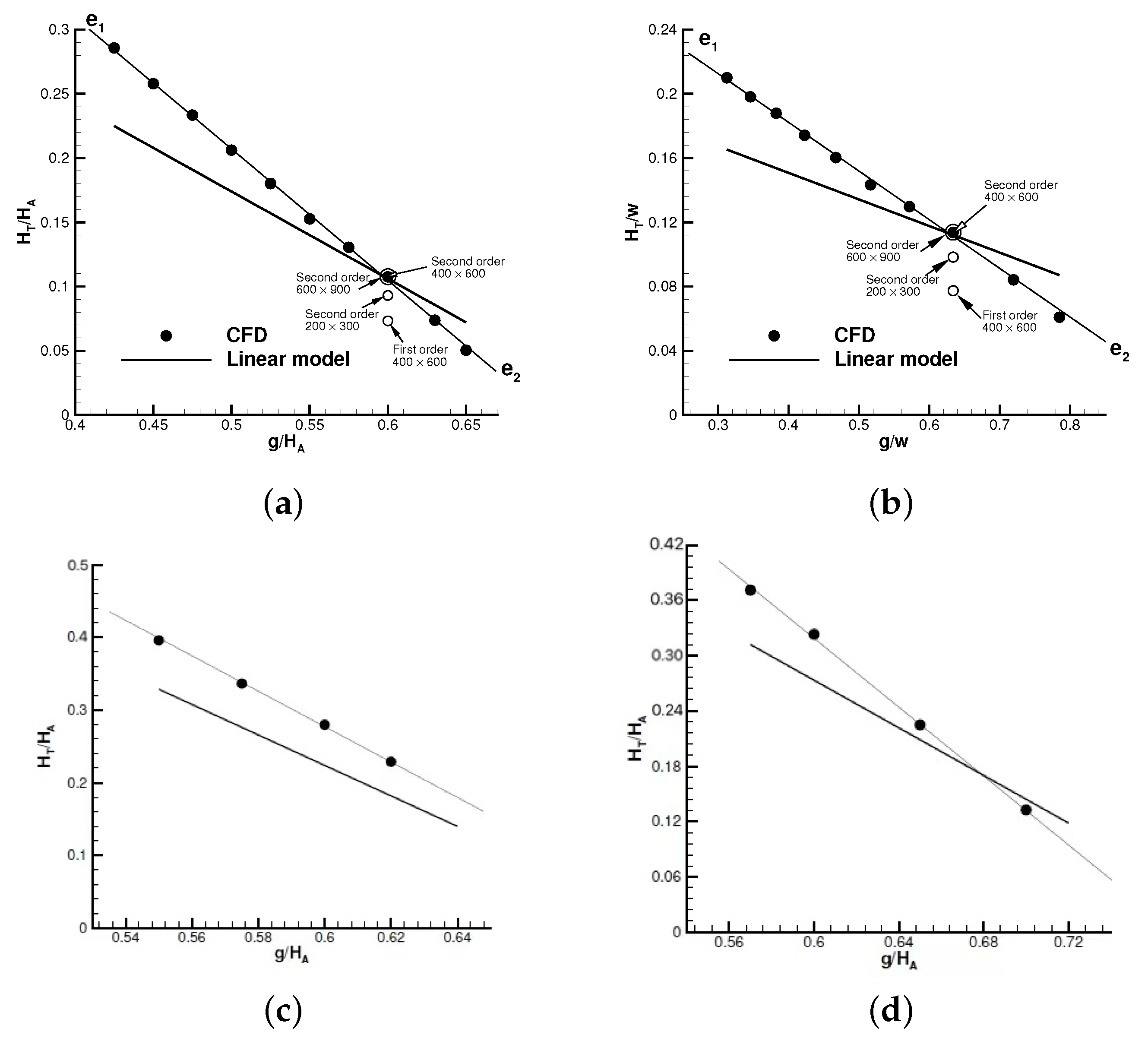
Now we display in Figure 3 the numerical results of normalized Mach stem height as a function of the normalized wedge trailing height for several different values of the inflow Mach number and wedge angle.

Figure 3a displays the variation of $\frac{H_T}{H_A}$ with respect to $\frac{g}{H_A}$, for $M_0=4$, ${\theta }_w={25}^{\circ }$ and a set of $\frac{g}{H_A}$ varying from $0.425$ to $0.65$. Figure 3b is the result for $\frac{H_T}{w}$ for various $\frac{g}{w}$, with $M_0=4$, ${\theta }_w={25}^{\circ }$ and a set of $\frac{g}{w}$ varying from $0.3124$ to $0.7849$. Figure 3c displays the variation of $\frac{H_T}{w}$ versus $\frac{H_A}{w}$ for $M_0=4$, ${\theta }_w={25}^{\circ }$ and a set of $\frac{H_A}{w}$ varying from $0.735$ to $1.2075$. The additional marks in Figure 3 show that numerical results with a grid of $400\times 600$ points and with second order of accuracy are acceptable since further refining the grid does not change the Mach stem height. This supports the previous claim that the use of a second-order method with the grid $400\times 600$ is accurate enough.

We observe that, for the conditions tested, the normalized Mach stem height $\frac{H_T}{H_A}$ is almost linear with respect to $\frac{g}{H_A}$, the normalized Mach stem height $\frac{H_T}{w}$ is almost linear with respect to $\frac{g}{w}$, and the normalized Mach stem height $\frac{H_T}{w}$ is almost linear with respect to $\frac{H_A}{w}$. In Figure 3, a straight line $e_1{e}_2$ is marked across the numerical data and this straight line is given by

$$\left\{\begin{array}{c}\frac{H_T}{H_A}=-1.0314\frac{g}{H_A}+0.7227,R^2=0.9994\hfill \\ \frac{H_T}{w}=-0.3087\frac{g}{w}+0.3054,R^2=0.9985\hfill \\ \frac{H_T}{w}=-0.3087\frac{H_A}{w}+0.4359,R^2=0.9985\hfill \end{array}\right.$$

where $R^2$ stands for the linear correlation coefficient.

The Mach contours for $M_0=4$, ${\theta }_w={25}^{\circ }$ and $\frac{g}{H_A}=0.425,0.475,0.525,0.575$ are displayed in Figure 4a–d. From the Mach contours, we can see how the Mach stem height decreases with increasing $\frac{g}{H_A}$. It is noted that when $\frac{g}{H_A}$ increases, the triple point moves in the downstream direction and the flow duct below the slipline is narrowed.

The linearity is also observed for another set of $M_0$ and ${\theta }_w$. Figure 5a displays the variation of $\frac{H_T}{H_A}$ with respect to $\frac{g}{H_A}$ for $M_0=4$, ${\theta }_w={30}^{\circ }$ and a set of $\frac{g}{H_A}$ varying from $0.55$ to $0.62$. Figure 5b displays the variation of $\frac{H_T}{H_A}$ with respect to $\frac{g}{H_A}$ for $M_0=3$, ${\theta }_w={25}^{\circ }$ and a set of $\frac{g}{H_A}$ varying from $0.57$ to $0.70$. In Figure 5, a straight line $e_1{e}_2$ is marked across the numerical data and this straight line is given by

$$\left\{\begin{array}{c}\frac{H_T}{H_A}=-2.3695\frac{g}{H_A}+1.6993,R^2=0.9996\hfill \\ \frac{H_T}{H_A}=-1.8537\frac{g}{H_A}+1.4308,R^2=0.9990\hfill \end{array}\right.$$

The numerical trend that the normalized Mach stem height decreases with increasing normalized trailing edge height seems to be counter-intuitive (and this trend has been demonstrated by Vuillon, Zeitoun and Ben-Dor [6] for a particular set of conditions), since apparently the Mach stem height should be proportional to the inlet height and one would expect the Mach stem height increase with increasing wedge trailing edge height. However, according to a simplified theoretical analysis given in Section 3, this trend can be justified.

3. A Simplified Analysis Showing Linearity of the Mach Stem Height with Geometry

Analytical models of various degrees of accuracy or complexity have been proposed in the past [16,20,21,22,23], none of which have been put into a linear form and have been used to predict the dependence of the Mach stem height on the wedge trailing length. Here, we derive an expression for the Mach stem height, which can be indeed put into a linear form. This expression is obtained by relating the sonic throat point c to the trailing edge R and to the triple point T, as done in previous works [16,20,21,22,23]. This analysis requires the slopes of the shock waves and of the slipline in the vicinity of the triple point as shown in Figure 6, as well as the slopes of the characteristic line $Rfc$ as marked in Figure 1. The method to estimate these slopes is given in Appendix A.

3.1. Preliminary Geometric Relations

Here, we establish geometric relations that relate the sonic throat position c to the trailing edge R through the characteristic line $Rfc$ (called the critical characteristic line) and to the triple point T through the slipline $Tbc$. Notations can be seen in Figure 1. The critical characteristic line brings the required pressure to the sonic throat c on the slipline to balance the critical pressure $p^{\ast }$ in the quasi-one-dimensional flow duct below the slipline.

The critical characteristic line $Rfc$ intersects with the reflected shock wave at point f and is composed of two segments $Rf$ and $fc$, both of which are assumed to be straight as by Bai and Wu [23]. Point f lies on the reflecting shock wave, which is generally curved according to Li and Ben-Dor [16]. Bai and Wu [23] gave a differential relation for the curved shape of this reflected shock. Here, for the purpose of evaluating the position of f within the present context of a simplified analysis, we omit the curvature of the shock segment $Tf$ and relate the position of f to the triple point as

$$y_f-y_T=(x_f-x_T)tan({\beta }_2^T-{\theta }_w)$$

(1)

where ${\beta }_2^T$ is the shock angle of the reflected shock wave as shown in Figure 6.

The position of point c at the sonic throat is related to the positions of the intersection point f and the trailing edge R by

$$\left\{\begin{array}{c}{y}_f-y_R=-(x_f-x_R)S_{Rf}\\ y_c-y_f=-(x_c-x_f)S_{fc}\end{array}\right.$$

(2)

where $S_{Rf}$ is the slope of the critical characteristic line $Rf$ upstream of the reflected shock wave and is determined by

$$S_{Rf}=tan({\theta }_f^{\ast }+{\mu }_f^{\ast })$$

(3)

and $S_{fc}$ is the slope of the transmitted critical characteristic line $fc$ which is given by

$$S_{fc}=tan({\theta }_r^{\ast }+{\mu }_r^{\ast }).$$

(4)

The parameters ${\theta }_f^{\ast }$ and ${\mu }_f^{\ast }$ are the flow deflection angle and Mach angle along the critical characteristic line $Rf$. The parameters ${\theta }_r^{\ast }$ and ${\mu }_r^{\ast }$ are the flow deflection angle and Mach angle along the critical characteristic line $fc$. The method to evaluate these parameters is given in Appendix A.

Solving (1) and (2) gives the following geometric relation that relates the sonic throat point c to the trailing edge R via the critical characteristic line $Rfc:$

$$L_1{y}_c+L_2{x}_c=O_1{y}_R+O_2{x}_R+N_1{y}_T+N_2{x}_T,$$

(5)

Here:

$$\left\{\begin{array}{c}{L}_1=1+\frac{S_{fc}}{\mathrm{\Psi }}+\frac{tan({\beta }_2^T-{\theta }_w)}{\mathrm{\Psi }}\hfill \\ L_2=S_{fc}+\frac{S_{fc}^2}{\mathrm{\Psi }}+\frac{S_{fc}tan({\beta }_2^T-{\theta }_w)}{\mathrm{\Psi }}\hfill \\ O_1=\frac{S_{fc}}{\mathrm{\Psi }}+\frac{tan({\beta }_2^T-{\theta }_w)}{\mathrm{\Psi }}\hfill \\ O_2=\frac{S_{Rf}{S}_{fc}}{\mathrm{\Psi }}+\frac{S_{Rf}tan({\beta }_2^T-{\theta }_w)}{\mathrm{\Psi }}\hfill \\ N_1=1\hfill \\ N_2=-tan({\beta }_2^T-{\theta }_w)\hfill \end{array}\right.$$

(6)

and:

$$\mathrm{\Psi }=tan({\mu }_f^{\ast }+{\theta }_f^{\ast })-tan({\mu }_r^{\ast }+{\theta }_r^{\ast })$$

(7)

Now, we establish a geometric relation that relates the sonic throat c to the triple point T through the slipline. This slipline is assumed to be composed of two segments $Tb$ and $bc$, where b is the intersection of the slipline and the leading characteristics $Rab$.

Since the intersection point b also lies on the leading characteristics $Rab$, we have the following geometric relations for point b:

$$\left\{\begin{array}{c}{y}_a-y_T=(x_a-x_T)tan({\beta }_2^T-{\theta }_w)\hfill \\ y_b-y_a=-(x_b-x_a)tan({\mu }_2^T+{\theta }_2^T)\hfill \\ y_a-y_R=-(x_a-x_R)tan({\mu }_1+{\theta }_w)\hfill \end{array}\right.$$

(8)

where ${\mu }_1=arcsin\frac{1}{M_1}$ and ${\mu }_2^T=arcsin\frac{1}{M_2^T}$ are the Mach angles. Solving (8) yields:

$$l_1{y}_b+l_2{x}_b=m_1{y}_R+m_2{x}_R+n_1{y}_T+n_2{x}_T$$

(9)

where:

$$\left\{\begin{array}{c}{l}_1=\frac{1}{{\mathrm{\Phi }}_{2}tan({\mu }_2^T+{\theta }_2^T)}+\frac{tan({\beta }_2^T-{\theta }_w)}{{\mathrm{\Phi }}_1}\hfill \\ l_2=\frac{1}{{\mathrm{\Phi }}_2}+\frac{tan({\beta }_2^T-{\theta }_w)tan({\mu }_2^T+{\theta }_2^T)}{{\mathrm{\Phi }}_1}\hfill \\ m_1=\frac{1}{{\mathrm{\Phi }}_{2}tan({\mu }_1+{\theta }_w)}+\frac{tan({\beta }_2^T-{\theta }_w)}{{\mathrm{\Phi }}_1}\hfill \\ m_2=\frac{1}{{\mathrm{\Phi }}_2}+\frac{tan({\mu }_1+{\theta }_w)tan({\beta }_2^T-{\theta }_w)}{{\mathrm{\Phi }}_1}\hfill \\ n_1=-1\hfill \\ n_2=tan({\beta }_2^T-{\theta }_w)\hfill \end{array}\right.$$

(10)

with:

$$\left\{\begin{array}{c}{\mathrm{\Phi }}_1=tan({\mu }_2^T+{\theta }_2^T)-tan({\mu }_1+{\theta }_w)\hfill \\ {\mathrm{\Phi }}_2=\frac{1}{tan({\mu }_1+{\theta }_w)}-\frac{1}{tan({\mu }_2^T+{\theta }_2^T)}\hfill \end{array}\right.$$

(11)

Gao and Wu (2010) found that the segment $Tb$ has some curvature due to secondary expansion waves which serve to balance the pressure change in the quasi-one-dimensional flow duct. Here, we omit this curvature in order to have an explicit relation between c and T. Notations can be seen in Figure 1.

Since b lies on $Tb$, which is treated to be a straight line, we have:

$$y_T-y_b=(x_b-x_T)tan{\delta }_s^T$$

(12)

Meanwhile, the slipline $bc$ is a curve that has a vanishing slope at point c (throat). We approximate $bc$ by a second order curve:

$$y-y_b=-(x-x_b)tan{\delta }_s^T+\tau {(x-x_b)}^2$$

(13)

Here, $\tau$ is a parameter ensuring that the second order curve has a vanishing slope at point c (throat), i.e., ${\left.\frac{dy}{dx}\right|}_{x=x_c}=0$, which, when (13) is used, gives $-tan{\delta }_s^T+2\tau (x_c-x_b)=0$, or:

$$\tau =\frac{tan{\delta }_s^T}{2(x_c-x_b)}$$

Using this value of $\tau$, (13) takes the following simple form:

$$y_c-y_b=-\frac{1}{2}(x_c-x_b)tan{\delta }_s^T$$

(14)

Solving (12) and (14) gives:

$$\left\{\begin{array}{c}{x}_b=\left(y_T-y_c\right)\frac{2}{tan{\delta }_s^T}+2x_T-x_c\hfill \\ y_b=2y_c-y_T-x_{T}tan{\delta }_s^T+x_{c}tan{\delta }_s^T\hfill \end{array}\right.$$

(15)

Now, putting (15) into (9) gives the geometric relation that relates the sonic throat to the triple point via the slipline:

$$X_1{y}_c+X_2{x}_c=Y_1{y}_R+Y_2{x}_R+Z_1{y}_T+Z_2{x}_T$$

(16)

where:

$$\left\{\begin{array}{c}{X}_1=2l_1-\frac{2l_2}{tan{\delta }_s^T}\hfill \\ X_2=l_{1}tan{\delta }_s^T-l_2\hfill \\ Y_1=m_1\hfill \\ Y_2=m_2\hfill \\ Z_1=l_1-\frac{2l_2}{tan{\delta }_s^T}+n_1\hfill \\ Z_2=l_{1}tan{\delta }_s^T-2l_2+n_2\hfill \end{array}\right.$$

(17)

In summary, the geometric relation (5) connects the sonic throat c to the trailing edge R following the critical characteristic line, and the relation (16) connects the sonic throat c to the triple point T following the slipline. They will be used to derive the expression for the Mach stem height below.

3.2. Mach Stem Height Expression Showing Linearity

In the following, we will use:

$$y_T=H_T,y_C=H^{\ast }=\frac{H_T}{\psi \left(M_m\right)},y_R=g,x_R-x_A=L=\frac{H_A-g}{tan{\theta }_w},x_A=0,y_A=H_A$$

(18)

Here, $H^{\ast }$ is the height of the sonic throat which can be related to the Mach stem height $H_T$ by the quasi-one-dimensional area Mach number relation $\frac{H_T}{H^{\ast }}=\psi \left(M_m\right)$ where:

$$\psi \left(M_m\right)=\frac{1}{M_m}{\left(\frac{2}{\gamma +1}\left(1+\frac{\gamma -1}{2}{M}_m^2\right)\right)}^{\frac{\gamma +1}{2(\gamma -1)}}$$

(19)

The triple point is on the incident shock wave, so that $y_A-y_T=\left(x_T-x_A\right)tan{\beta }_1$, meaning that:

$$x_T=x_A+\frac{y_A-y_T}{tan{\beta }_1}$$

(20)

For $x_A=0$, the expression (20) simplifies to:

$$x_T=\frac{H_A-H_T}{tan{\beta }_1}$$

(21)

Solving (5) and (16) gives:

$$Q{y}_c=C_1{y}_R+C_2{x}_R+D_1{y}_T+D_2{x}_T$$

(22)

where:

$$\left\{\begin{array}{c}Q=X_2\frac{L_1}{L_2}-X_1\hfill \\ C_1=X_2\frac{O_1}{L_2}-Y_1\hfill \\ C_2=X_2\frac{O_2}{L_2}-Y_2\hfill \\ D_1=X_2\frac{N_1}{L_2}-Z_1\hfill \\ D_2=X_2\frac{N_2}{L_2}-Z_2\hfill \end{array}\right.$$

(23)

Using (21) to replace $x_T$ in (22), we obtain:

$$Q{y}_c=C_1{y}_R+C_2{x}_R+\left(D_1-\frac{D_2}{tan{\beta }_1}\right)y_T+D_2{x}_A+\frac{D_2}{tan{\beta }_1}{y}_A$$

(24)

Putting (18) into (24) yields:

$$\left\{\begin{array}{c}\frac{H_T}{H_A}=A(M_0,{\theta }_w)\frac{g}{H_A}+B(M_0,{\theta }_w)\hfill \\ A(M_0,{\theta }_w)=\frac{C_1-\frac{C_2}{tan{\theta }_w}}{\frac{Q}{\psi \left(M_m\right)}-D_1+\frac{D_2}{tan{\beta }_1}}\hfill \\ B(M_0,{\theta }_w)=\frac{\frac{C_2}{tan{\theta }_w}+\frac{D_2}{tan{\beta }_1}}{\frac{Q}{\psi \left(M_m\right)}-D_1+\frac{D_2}{tan{\beta }_1}}\hfill \end{array}\right.$$

(25)

The expression (25) indeed shows the linearity of $\frac{H_T}{H_A}$ with respect to $\frac{g}{H_A}$, for fixed $M_0,{\theta }_w$. This linearity has been observed in numerical simulation, as shown in Figure 3a.

If we introduce the obvious geometric relation $H_A=g+wsin{\theta }_w$ into (25), we obtain an equivalent form:

$$\left\{\begin{array}{c}\frac{H_T}{w}=D^{\left(k\right)}(M_0,{\theta }_w)\frac{g}{w}+E^{\left(k\right)}(M_0,{\theta }_w)\hfill \\ D^{\left(k\right)}=A^{\left(k\right)}(M_0,{\theta }_w)+B^{\left(k\right)}(M_0,{\theta }_w)\hfill \\ E^{\left(k\right)}=B^{\left(k\right)}(M_0,{\theta }_w)sin{\theta }_w\hfill \end{array}\right.$$

(26)

which shows the linearity of $\frac{H_T}{w}$ with respect to $\frac{g}{w}$, for fixed $M_0,{\theta }_w$. This linearity was observed in numerical simulation, as shown in Figure 3b.

If we put $g=H_A-wsin{\theta }_w$ into (26), we obtain another equivalent form:

$$\frac{H_T}{w}=D^{\left(k\right)}(M_0,{\theta }_w)\frac{H_A}{w}+E^{\left(k\right)}(M_0,{\theta }_w)$$

(27)

where $E^{\left(k\right)}=B^{\left(k\right)}(M_0,{\theta }_w)sin{\theta }_w$. Thus, if normalized inlet height $\frac{H_A}{w}$ is used as an input parameter representing geometry, $\frac{H_T}{w}$ is still a linear function of $\frac{H_A}{w}$, for fixed $M_0$ and ${\theta }_w$. This linearity has been observed in numerical simulation, as shown in Figure 3c. Note that Li and Ben-Dor [16] considered a situation where the wedge length w is fixed and the height g is increased, and showed that the foot of the Mach stem follows a linear trajectory. This observation, which they pointed out needs to be explained, may be associated with the linearity pointed out by the present work.

3.3. Assessment of the Accuracy of the Mach Stem Height Expression

The Mach stem height expressions (25)–(27) were obtained under some simplifications as stated in Appendix A. It is thus interesting to see whether these are also accurate enough for quantitative prediction. Here, we will assess their accuracy by comparing them with previous results and the present CFD data.

The experimental data of Hornung and Robinson [18] are usually used for comparison. Here, we consider their case with $M_0=3.98$ and $g/w=0.4$, with the varying incident shock angle (${\beta }_1$). Figure 7 displays the comparison of the Mach stem height expression (25) with some various previous works. In Figure 7, the experimental data of Hornung and Robinson [18] and Mouton and Hornung [27], and the CFD data of Mouton and Hornung [21], and Vuillon et al. [6] are displayed. It can be seen that the expression (25) provides a curve lying between the curves of Bai and Wu [23] and Gao and Wu [22].

The comparison of linear expression (25) with the present numerical solutions (already shown in Figure 3a–c and Figure 5a,b of Section 2) is given in Figure 8a–e. It is seen that, though the expression (25) displays linearity as CFD simulation, the slopes of the linear curves signficantly differ from the CFD results.

3.4. Summary and Significance of the Linear Analysis

The linearity predicted in the present simplified analysis appears to suggest that the linearity observed in the CFD simulation for a finite number of input parameters has some generality.

A comparison of the linear model (25) obtained from the simplified analysis of CFD data suggests that the slope, say $\frac{A(M_0,{\theta }_w)}{B(M_0,{\theta }_w)}$, in the linear curve does not yet have the required accuracy to be comparable with CFD data. The factors A and B in the expression (25) thus need elaboration before the expression (25) can be used for accurate prediction.

Despite the difference between the slope in the model (25) and the slope in CFD results, the agreement of linearity is meaningful in the future study of model elaboration since in the suggested linear model, the influence of wedge height and the influence of the inflow Mach number $M_0$ and wedge angle ${\theta }_w$ are separate. For model elaboration, one can focus on working out more accurate A and B, which only depend on the inflow Mach number $M_0$ and wedge angle ${\theta }_w$. Moreover, even without knowing the exact values of the linear coefficients A and B, the conclusion that the normalized Mach stem height is linear with respect to the normalized wedge height is already useful in specific application to consider the precise influence of geometry, since one can just perform numerical or experimental work for the two sets of wedge height to fit the values of the slope in the linear model and then apply this linear model to predict the Mach stem height for other wedge height. This could greatly reduce the cost.

4. Conclusions

In this paper, we considered the dependence of the Mach stem height on the geometry when the geometry parameter (such as the trailing edge height) has a wide range. Such a study complements the past studies since many of the previous studies have focused on a narrow range of geometry.

Numerical simulation showed that the normalized Mach stem height is almost linear with respect to the normalized trailing edge height, independently of how they are normalized. When the trailing edge height is increased, keeping the inflow Mach number and the wedge angle fixed, the triple point moves in the downstream direction and the flow region between the slipline and the reflected surface is narrowed.

A simplified analysis showed that the linearity observed in CFD could be explained. This analysis leads to an expression of the normalized Mach stem height with respect to the normalized trailing edge height, which has the linear form $\frac{H_T}{H_A}=A\frac{g}{H_A}+B$ or $\frac{H_T}{w}=A\frac{g}{w}+B$. The coefficients A and B only depend on the inflow Mach number and the wedge angle.

The present work suggested that a Mach stem height model can be expressed as a linear function of the geometry. Further work could be done by working out more accurate coefficients A and B for purpose of quantitative prediction. In a specific application to consider the precise influence of geometry, one can also perform numerical or experimental work for two sets of wedge height to fit the values of the slope in the linear model and then apply this linear model to predict the Mach stem height for other wedge height.

References

1. Ben-Dor, G. Shock Wave Reflection Phenomena; Springer: Berlin/Heidelberg, Germany, 2007. [Google Scholar]
2. Henderson, L.F.; Lozzi, A. Experiments on transition of Mach reflection. J. Fluid Mech. 1975, 68, 139–155. [Google Scholar] [CrossRef]
3. Bazhenova, T.V.; Fokeev, V.P.; Gvozdeva, L.G. Regions of various forms of Mach reflection and its transition to regular reflection. Acta Astronaut. 1976, 3, 131–140. [Google Scholar] [CrossRef]
4. Hornung, H.G.; Oertel, H.; Sandeman, R.J. Transition to Mach reflection of shock waves in steady and pseudo-steady flows with and without relaxation. J. Fluid Mech. 1979, 90, 541–560. [Google Scholar] [CrossRef] [Green Version]
5. Teshukov, V.M. On stability of RR of shock waves. Prikl. Mekh. Technol. Fiz 1989, 2, 26–33. [Google Scholar]
6. Vuillon, J.; Zeitoun, D.; Ben-Dor, G. Reconstruction of oblique shock wave reflection in steady flows. Part 2. Numerical investigation. J. Fluid Mech. 1995, 301, 37–50. [Google Scholar] [CrossRef]
7. Chpoun, A.; Passerel, D.; Li, H.; Ben-Dor, G. Reconsideration of the oblique shock wave reflection in steady flows. Part 1. Experimental investigation. J. Fluid Mech. 1995, 301, 19–35. [Google Scholar] [CrossRef]
8. Li, H.; Ben-Dor, G. Application of the principle of minimum entropy production to shock wave reflections. I. Steady flows. J. Appl. Phys. 1996, 80, 2027–2037. [Google Scholar] [CrossRef]
9. Ivanov, M.S.; Ben-Dor, G.; Elperin, T.; Kudryavtsev, A.N.; Khotyanovsky, D.V. Flow–Mach-number-variation-induced hysteresis in steady flow shock wave reflections. AIAA J. 2001, 39, 972–974. [Google Scholar] [CrossRef]
10. Ben-Dor, G.; Ivanov, M.; Vasilev, E.I.; Elperin, T. Hysteresis processes in the regular reflection to Mach reflection transition in steady flows. Prog. Aerosp. Sci. 2002, 38, 347–387. [Google Scholar] [CrossRef] [Green Version]
11. Hornung, H. Mach reflection in steady flow. I. Mikhail Ivanovs contributions, II. Caltech stability experiments. AIP Conf. Proc. AIP Publ. 2014, 1628, 1384–1393. [Google Scholar]
12. Courant, R.; Friedrichs, K.O. Supersonic Flow and Shock Waves; Wiley-Interscience: Hoboken, NJ, USA, 1948. [Google Scholar]
13. Liepmann, H.; Roshko, A. Elements of Gasdynamics; John Wiley and Sons: Hoboken, NJ, USA, 1957. [Google Scholar]
14. Emanuel, G. Gasdynamics: Theory and Applications; American Institute of Aeronautics and Astronautics: New York, NY, USA, 1986. [Google Scholar]
15. Ben-Dor, G.; Takayama, K. The phenomena of shock wave reflection-a review of unsolved problems and future research needs. Shock Waves 1992, 2, 211–223. [Google Scholar] [CrossRef]
16. Li, H.; Ben-Dor, G. A parametric study of Mach reflection in steady flows. J. Fluid Mech. 1997, 341, 101–125. [Google Scholar] [CrossRef]
17. Chow, W.L.; Chang, I.S. Mach reflection associated with over-expanded nozzle free jet flows. AIAA J. 1975, 13, 762–766. [Google Scholar] [CrossRef]
18. Hornung, H.G.; Robinson, M. Transition from regular to Mach reflection of shock waves Part 2. The steady-flow criterion. J. Fluid Mech. 1982, 123, 155–164. [Google Scholar] [CrossRef]
19. Schmisseur, J.; Gaitonde, D. Numerical simulation of Mach reflection in steady flows. Shock Waves 2011, 21, 499–509. [Google Scholar] [CrossRef]
20. Azevedo, D.J.; Liu, C.S. Engineering approach to the prediction of shock patterns in bounded high-speed flows. AIAA J. 1993, 31, 83–90. [Google Scholar] [CrossRef]
21. Mouton, C.A.; Hornung, H. Mach stem height and growth rate predictions. AIAA J. 2007, 45, 1977–1987. [Google Scholar] [CrossRef]
22. Gao, B.; Wu, Z.N. A study of the flow structure for Mach reflection in steady supersonic flow. J. Fluid Mech. 2010, 656, 29–50. [Google Scholar] [CrossRef]
23. Bai, C.Y.; Wu, Z.N. Size and shape of shock waves and slipline for Mach reflection in steady flow. J. Fluid Mech. 2017, 818, 116–140. [Google Scholar] [CrossRef]
24. Roy, S.; Gopalapillai, R. An analytical model for asymmetric Mach reflection configuration in steady flows. J. Fluid Mech. 2019, 863, 242–268. [Google Scholar] [CrossRef]
25. Lin, J.; Bai, C.Y.; Wu, Z.N. Study of asymmetrical whock wave reflection in steady supersonic flow. J. Fluid Mech. 2019, 864, 848–875. [Google Scholar] [CrossRef]
26. Roe, P. Characteristic based schemes for the Euler equations. Annu. Rev. Fluid Mech. 1986, 18, 337–365. [Google Scholar] [CrossRef]
27. Mouton, C.A.; Hornung, H. Experiments on the mechanism of inducing transition between regular and Mach reflection Mach stem height and growth rate predictions. Phys. Fluids 2008, 20, D541–D572. [Google Scholar] [CrossRef] [Green Version]
28. Von Neumann, J. Oblique Reflection of Shock; Explos. Res. Rep. 12 Navy Dept.; Bureau of Ordinance: Washington, DC, USA, 1943. [Google Scholar]
Figure 1. Mach reflection configuration. The inflow Mach number M 0 , the wedge angle θ w , the inlet height H A and the lower wedge surface length w or the trailing edge height g are given conditions.
Fluids 06 00313 g001
Figure 2. Mach number contours for M 0 = 4 , θ w = 25 and g H A = 0.6 : (a) first order with a 400 × 600 mesh; (b) second order with a 200 × 300 mesh; (c) second order with a 400 × 600 mesh; and (d) second order with a 600 × 900 mesh.
Fluids 06 00313 g002
Figure 3. Numerical results for normalized Mach stem heights as a function of the normalized wedge trailing edge height for M 0 = 4 and θ w = 25 : (a) H T H A versus g H A ; (b) H T w versus g w ; (c) H T w versus H A w . The line e 1 e 2 is a straight line passing through the CFD data. Open circles are CFD data obtained using grids different to 400 × 600 points or a first-order accurate method.
Fluids 06 00313 g003
Figure 4. Numerical results for Mach contours with M 0 = 4 and θ w = 25 : (a) g H A = 0.425 ; (b) g H A = 0.475 ; (c) g H A = 0.525 ; and (d) g H A = 0.575 .
Fluids 06 00313 g004
Figure 5. Numerical results for normalized Mach stem heights as a function of the normalized wedge trailing edge height: (a) H T H A versus g H A for M 0 = 4 and θ w = 30 ; (b) H T H A versus g H A for M 0 = 3 and θ w = 25 .
Fluids 06 00313 g005
Figure 6. Triple point solution.
Fluids 06 00313 g006
Figure 7. Comparison of the linear model (25) against previous authors for M 0 = 3.98 and g / w = 0.4 .
Fluids 06 00313 g007
Figure 8. Comparison between the linear model (25) and CFD data: (a) H T H A versus g H A for M 0 = 4 , θ w = 25 ; (b) H T w versus g w for M 0 = 4 , θ w = 25 ; (c) H T H A versus g H A for M 0 = 4 , θ w = 30 ; (d) H T H A versus g H A for M 0 = 3 , θ w = 25 ; and (e) H T w versus H A w for M 0 = 4 , θ w = 25 .
Fluids 06 00313 g008aFluids 06 00313 g008b
Publisher’s Note: MDPI stays neutral with regard to jurisdictional claims in published maps and institutional affiliations.