Open Water Flume for Fluid Mechanics Lab

Abstract

Open water flume tanks with closed-loop circulation driven by centrifugal pumps are essential for hydro experimentation in academic settings as well as research centers. The device is also attractive due to its versatility and easy-to-maintain characteristics. Nevertheless, commercial open flume systems can be expensive and become less prioritized in engineering schools. This paper describes the design and fabrication of an affordable, medium-size water flume tank, suitable for education purposes. The central piece of the system is a transparent observation chamber where fluid experiments are typically conducted and observed. The expected maximum average water speed in the observation chamber of about 60 cm per second was achieved by the inclusion of a 3 hp centrifugal pump. The size and capacity of the current design were constrained by space limitation and available funds. The educational facility was assigned as a two-semester multi-disciplinary capstone senior design project incorporating students and faculty of mechanical, electrical, and computer engineering programs in our campus. The design process provides a training platform for skills in the area of Computer Aided Designs (CAD), Finite Element Analysis (FEA), Computational Fluid Dynamics (CFD), manufacturing, and experimentation. The multi-disciplinary project has contributed to the improvement of soft skills, such as time management, team working, and professional presentation, of the team members. The total material cost of the facility was less than USD 6000, which includes the pump and its variable frequency driver. The project was made possible due to the generous sponsor of the Vibration Institute.

1. Introduction

Open water flumes provide effective hands-on multidisciplinary learning tools for students matriculated in engineering programs, as well as in the physical education program [1]. Senior students participating in the design and fabrication process of the flume obtained the opportunity to reinforce fundamental engineering concepts and to master valuable technical skills [2,3,4]. The reported open flume was motivated by the need of a test chamber for an ongoing research on bladeless turbines, as well as the desire to have such device in the fluid mechanics laboratory. The current design was inspired by a small scale commercial water flow tank used in the investigation of vortex-induced autorotation and oscillation of straight cylinders [5,6], as well as the energy potential from such vibration modes of symmetric geometries [7,8]. Open channel tanks are paramount for various hydrodynamic research areas, such as designs of hydrokinetic energy harvesters, investigation of flow characteristics in the presence of obstacles, drag and lift of objects exposed to fluid flows, etc. The vortex-induced vibration (VIV) of objects exposed to flow has emerged as attractive potential sources of renewable energy. Additionally, the versatility of open channel flumes has allowed plethora of vibration modes to be experimented. Sun et al. used a 40 cm wide and long rectangular channel to convert vortex-induced vibration and galloping of blunt bodies into electricity via piezoelectric strips [9]. In a small scale water tank, Cao et al. attempted to amplify the vibration amplitudes of piezoelectric strips by means of magnet fields [10,11]. Arionfard and Nishi utilized a small (30 cm × 1 m) water channel to investigate power harnessing potential of pivoted cylinder exposed to highly turbulent flow [12]. The utilization of much larger size channels allows modeling of near-realistic flow and full-scale energy harvesters. Rostami and Fernandes studied the energy harvesting from the torsional galloping, fluttering, and autorotation modes of flat and S-shape plates using a 1.4 m, wide 22 m long water channel [13,14,15,16]. Furthermore, a 1 m wide water flume tank is used in the development of VIVACE (Vortex-Induced Vibration of Aquatic Clean Energy), which exploits the transverse-to-the-flow (lateral) oscillation mode of VIV at large range of Reynolds numbers using magnets attached to cylindrical bars as harvesters [17,18,19]. An open channel with similar width but five times longer (about 42 m long) was recently used in the attempts to utilize the galloping modes of triangular cylindrical bars at much higher velocity [20,21]. Generally, interests in the designs of innovative hydrokinetic energy turbines have been well facilitated by open water flumes. The facility is adaptable for various types of turbines and its blades, as well as a range of measurement needs. Barber et al. studied the power and thrust improvement of axial turbines after the utilization of carefully designed adaptive pitch composite blades [22]. A small commercial flow loop water tank was used in the investigation of wake behind the propellers of wind turbines [23]. Open water flume experimentations of vertical axis hydrokinetic generators, such as Savonius and Darrieus turbines, have been intensified lately. These turbines are attractive renewable energy harvesters due to their simple designs, low-cost manufacturing, easy maintenance, and independence of flow direction. Talukdar et al. demonstrated that the performance of two-bladed semi-circular Savonius turbines is better than two-bladed elliptical and three-bladed semi-circular designs [24]. On the other hand, Sarma et al. pointed out that the three-bladed Savonius model performs better in water than in air flow [25]. It is interesting to note that placing an upstream obstacle can improve the performance of a modified two-bladed Savonius turbines [26] and Darrieus turbines [27]. Attempts to assemble and test the two turbines into one single hybrid unit have shown promising outcomes [28,29]. In the hydrology area, large size tanks facilitate investigations of particle sedimentation carried by water flow [30], improvement of hyporheic zones due to riverbed restoration [31], and effects of flood waves on river banks [32] among many other studies. The open channel allows examination of flow qualities, such as head loss and turbulence, by placing out obstacles in its test section. Investigation of the head loss due to the presence of submerged baffle-posts [33,34] and examination of water turbulence due to rib roughness [35] are examples of important studies to be carried out for better irrigation systems. Examinations on the interaction between vegetation and water flows shed light on the life quality of river. Here, the vegetation under investigation is carefully arranged along the base of the test chamber and its effects on water waves are studied using camera [36]. Lastly, we would like to mention flume experimentations to test the drag and lift of 3D-printed models of swimmers [1] that show the capability of water flume to accommodate large range of multidisciplinary applications. The transparent chamber of the flume certainly allows flow measurement by either direct observation [33,34] or flow visualization technology such as dye injection [31], hydrogen bubble [37], particle image velocimetry (PIV) [23,37,38], planar laser-induced fluorescence (PLIF) [39], stereoscopic digital particle image velocimetry (SDPIV) [40], laser doppler velocimetry (LDV), and acoustic doppler velocimetry (ADV) [30] methods. It is obvious that the versatility and easy-to-maintain characteristic of the open flume systems makes the device very attractive to be included in fluid mechanics and hydrology labs.

The presented work discusses the design and fabrication of a small size (15 cm wide and 75 cm long test chamber) open water flume with closed flow loop driven by a 3 hp centrifugal pump. The designs must consider limited funds, available space in the lab, and mobility requirement. The overall size of the system, the materials for the structural frame and the chambers, as well as the pump selection, can be determined by the flow requirement in the observation chamber and experiments that would be conducted. In this project, the maximum fund was set to be USD 10,000 and the overall size is governed by the size of the freight elevator in the school. The overall length of the system must be kept to about 2.5 m or shorter, so that it can fit in the school’s freight elevator. Reported in this paper are the pump selection process, structural analysis of the supporting frame, computational fluid dynamic analysis of the flume, manufacturing process, and conducted experimentations on the flow visualization using dye injection and investigation of drag forces on submerged objects. A brief discussion on the budget is presented before the paper is closed with a discussion and conclusion sections.

2. Basic Design and Pump Selection

This water flow tank is designed to provide straight uniform flow with an average speed of as much as 60 cm/s through its transparent observation chamber. The cross-sectional dimension of the observation chamber is planned to be at least 15 × 15 cm². The length of the observation chamber was designed to be 60 cm. This length is needed to provide enough observation room for vortex trail and wakes behind objects exposed to water flow. The final length of the test chamber is 75 cm. The selection of the maximum speed and chamber dimension was based on a commercial water flume used in experiments on vortex-induced oscillation of cylinders [41]. An upstream manifold in a shape of converging chamber of about 44 cm is added to provide room for the water to reduce its turbulence and complex characteristics prior to enter the observation chamber. The height of the observation chamber was designed to be ~1.2 m, a little less than the average height of human eyes of ~1.4 m. The top side of the observation chamber is expected to be open to allow direct physical access to the flow and, more importantly, easy placement of objects exposed to the flow. Tight covering of the top side to achieve high speed of water flow is possible, but the pressure increase must carefully be calculated. The flow tank was designed to be mobile, so that it can be easily moved when needs arise. The overall length and width of the flow tank therefore is constrained to size of the school’s freight elevator of approximately 2.16 by 2.44 m². This size put limitation on the total length of the equipment to be about 2.5 m. The overall budget of this device is set to be less than USD 10,000, based on the maximum fund by the sponsor for this project: Vibration Institute. As the project is scheduled for a senior design project, the design and construction must be finished in two semesters.

The design process begins with a preliminary calculation for the pump specification, which would determine the pipe diameters, the dimension of supporting frames, and required power outlet. Detail calculation would require flowrates, height of the observation chamber, lengths, diameters, and materials of various pipes involved in the designs, as well as connections and pipe bends. In the absence of many of these parameters, the needed pump power can be calculated using the required flowrates and maximum elevation that needs to be overcome by the water. Other parameters need to be estimated. 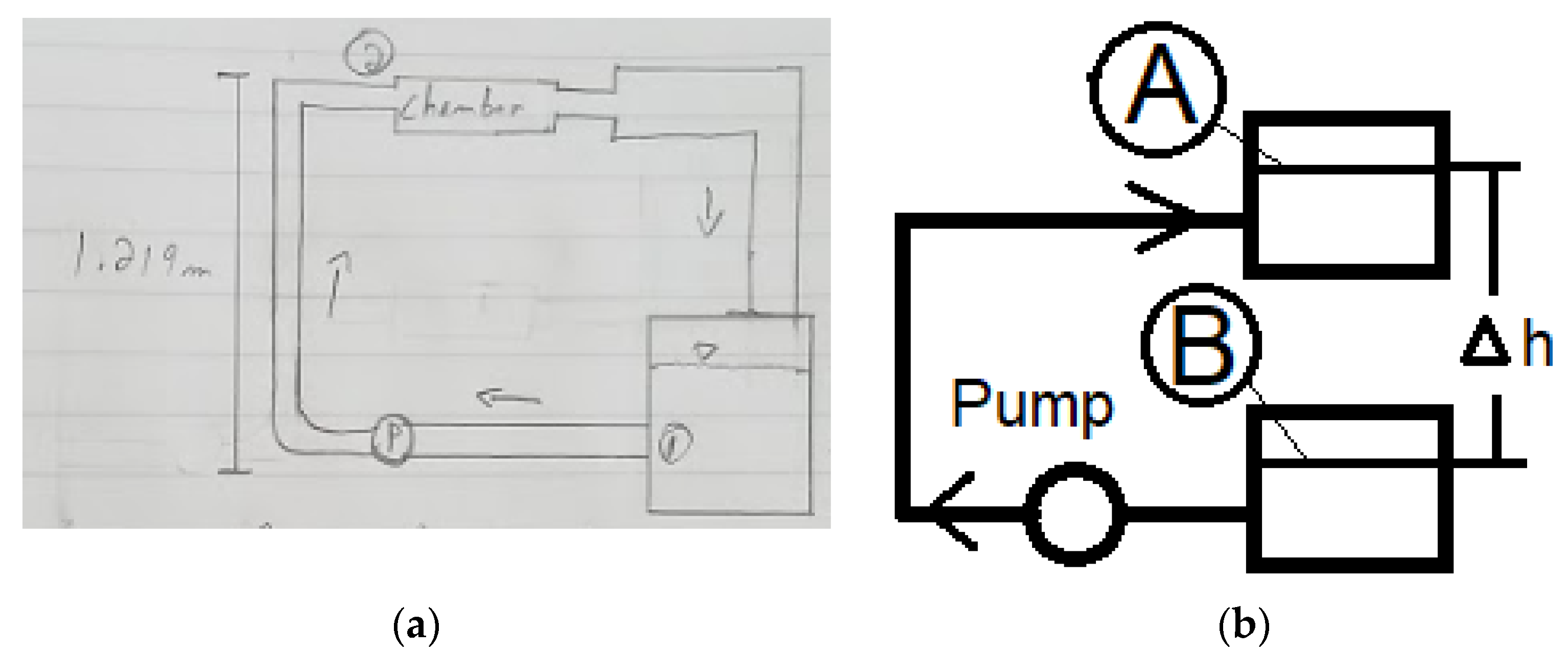Figure 1 panel (a) shows an example of simple conceptual sketch of the water flow system drawn by students involved in this project. The flowrate can be determined from the demanded speed $\overline{V}$ of ~0.6 m/s and cross section area of the observation chamber of $A=0.15\times 0.15=0.0225 {\mathrm{m}}^2$, through the equation for flowrate $Q=\overline{V}\times A=0.0135{\mathrm{m}}^3/\mathrm{s}$, or about 12,800 gph or 214 gpm. Figure 1 panel (b) depicts a simple open flow diagram to represent the design of the water tank. The pump must overcome the height of the observation chamber and resistance by all pipes and chambers (major losses) and various connections (minor losses) along the loop. Note also that the effects of gravity on the returning channel from the observation chamber is not included in the calculation, as the power discount may not be significant. The flow diagram shown in Figure 1 guides us in determining the Bernoulli equation to be used.

The total head $h_p$ for the calculation of pump power can be obtained from the Bernoulli equation easily found in fluid mechanics text books [42,43];

$$h_p=\mathsf{\Delta }h+\mathsf{\Sigma } f\frac{L}{D}\frac{{\overline{V}}^2}{2g}+\mathsf{\Sigma } K\frac{{\overline{V}}^2}{2g}$$

(1)

The $\mathsf{\Delta }h$ represents the elevation difference between two end points in the flow diagram. In our case, we would take this as the largest height difference available in the water tank system, which is the height of the observation chamber. The second and third terms in the equation are known as the major and minor losses, losses that are caused by the wall friction along the pipes and channels in the system, and losses that are caused by any other obstacles in the system, respectively. For the major loss, the Darcy’s friction factor $f$ is known to depend on the Reynolds numbers of the flow and roughness of the pipe. The $L$ and $D$ are length and diameter of pipe, respectively. In the third term, the constant $K$ represents resistance factors for various obstacles along the loop, such as bends, junctions, entrances, etc. The Reynolds number is defined as

$$Re=\frac{\rho \overline{V}D}{\mu }$$

(2)

where $\rho$ and $\mu$ are the water density and absolute viscosity, respectively. In calculating the major and minor losses, the average speed $\overline{V}$ of the water should be taken at each section along the pipe where the loss is calculated, and the $D$ represents hydraulic diameter of that particular section. As the detail geometry of the flume is not yet known, we assume the contribution of these losses to be simply double the elevation difference, hence the total head is $h_p=1.2+2\times 1.2=3.6 \mathrm{m}$. It will be shown later that this estimation is larger than an alternative estimation based on possible major and minor losses in the flume. The required pump power can be calculated using [42,43]

$$W_p=\frac{\rho g Q h_p}{\eta }$$

(3)

In estimating the needed pump power, we took the density ($\rho$) and absolute viscosity ($\mu$) of water at atmospheric pressure and 20 °C to be 998 kg/m³ and 0.001 Pa.s [43,44], respectively, while the gravitational constant $g=9.81$ m/s². Not knowing the pump to be purchased yet, we estimated the pump efficiency $\eta$ from commercial pump examples presented in textbooks [43,44]. Based on these examples, for the required flow rate of 214 gpm, the efficiency was found to be about $\eta \approx 60\%$. Using these data, we can estimate the required pump power to be only $W_p=793 \mathrm{W}$ or about 1.06 hp. Note that the power calculation here is based on high flow rate but very low head loss, due to the very short pipe and minimal height involved in the current design. Consequently, such a pump, with such combination of low pump power and high flow rate, may not be available in the market. Here, students need to realize that the market availability of the pump puts a constraint in the design.

Alternatively, the major and minor losses could be estimated based on the possible materials and components to be used in the designs. This detail calculation process provides valuable realistic exercise for the students involved in this project.

Table 1. List of friction and major head loss of pipes and channels involved in the designs.

Materials	Length (m)	Diameter (m)	Roughness (mm)	$\overline{\mathit{V}}$ (m/s)	Re	f	$\mathit{h} \left(\mathbf{m}\right)$
Plexiglass	0.6	$0.15\times 0.15$	0.0015	0.6	100,921	0.018	0.001
Stainless Steel	4.0	$~0.4\times 0.3$	0.002	0.11	49,339	0.021	<<0.001
Plastics	1.0	$\pi \times {0.05}^2$	Smooth	1.7	95,315	0.017	0.05

shows list of pipes and channels, as well as estimated major head losses. The mean velocity for each section is estimated from the flowrate of 0.0135 m³/s based on the required flow speed of 60 cm/s. The major loss is defined as $h=f\frac{L}{D}\frac{{\overline{V}}^2}{2g}$ and the friction factor for each section is determined from the Moody chart based on the associated Reynolds number and given roughness factors of the pipes [42,43,44,45]. Due to the short pipes involved in this design, this calculation renders net head much less than 1 m, well below the estimated head mentioned before. As expected, the required head is dominated by the height of the water column that must be overcome.

Similarly, the minor losses can be estimated by considering all possible pipe components that are to be included in the system and evaluate its contribution.

Table 2. In this table, we list of possible minor loss components to be included in the design.

Components	Amount	K
Ball valve	1	0.05
Couplings	7	0.08
Entrances	6	0.5
Sudden Expansion	1	0.5

shows the list of possible components to be installed in the system and its corresponding “K” values obtained from a textbook [42,45]. The total $K$ value is about 4, and this results in minor head loss of about 0.2 m, after assuming velocity of 1 m/s. Combined with the major head loss calculated above, the total would still be less significant compared to the head by elevation difference.

Three (3) pumps for minimum 190 gpm flow rate are selected from McMaster–Carr [46]; (A) High-Efficiency Circulation Pumps for Water, Coolants, and Oil, (B) Harsh-Environment Self-Priming Circulation Pumps for Water and Coolants, and (C) High-Flow Inline Circulation Pumps for Water. Shown in

Table 3. List of potential centrifugal pumps available in McMaster–Carr and its working fluid, maximum flow rate, power requirement, maximum head, and unit price.

Pump #	Product Name	Working Fluid	Max. Flow Rate (gpm)	Power (hp)	Maximum Head (m)	Price (USD, 2018)
A	High-efficiency Circulation Pumps	Water, coolants, oil	190	5	19	~1800
B	High-Flow Harsh-Environment Circulation Pump	Water, coolants	375	3	20	~1105
C	High-Flow Inline Circulation Pumps for Water	Water only	240	3	14.6	~2100

are features of the three pumps considered for the system. The price range is approximately USD 1000 to 2000 (2018 price). The specification of these pumps shows that the flow rates and power requirement slightly above our design requirement and the prices are within the budget range.

In selecting the pump, students may be asked to setup a simple decision matrix. The matrix allows a group of students to quantify their opinions on factors that weigh the buying decision such as price, capacity, pump power, and type of fluids that can be handled by the pump. In using the matrix, each student in the design team gives score between 1 to 3 (as there are three pump candidates), indicating the level of preference, for each category. For example, a student who prefers to buy pump B as they think that the price is the most reasonable, not necessarily the cheapest, should score 3 for pump B under the category of “Price”. If the student considers that they prefer another pump for the power, then they can put a score of either 2 or 1 under the “Power” category for pump B. Students involved in the pump selection process collect their matrix, and the pump with highest total score should be selected.

Table 4. An example of decision matrix for pump selection process. Each student involved in the project may participate in the selection process by filling out this table.

Product	Working Fluid	Flow Rate	Power	Maximum Head	Price	Total Score
A	1	1	3	2	2	9
B	3	2	2	3	3	13
C	2	3	1	1	1	8

shows an example of such decision matrix performed by one student. This example shows that the student preferred to purchase pump B over the other two pumps.

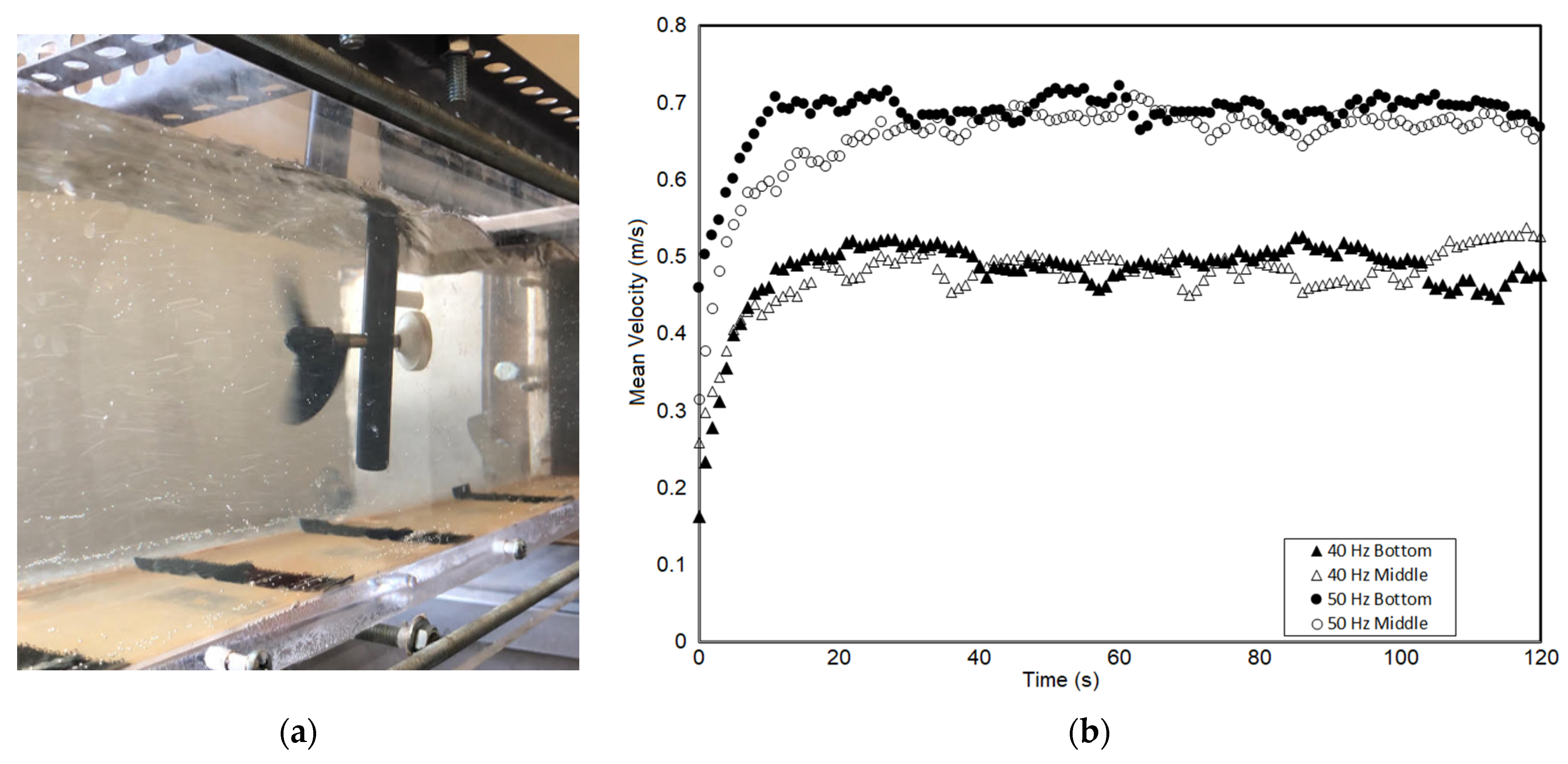
The selected 3″-self-priming pump is manufactured by AMT, a Gorman–Rupp Company based in Mansfield, OH, USA [47]. This is a 3-phase pump that draws 10 Amps at 208–230 V. The stainless-steel impeller is encased in cast iron and capable of delivering 375 gpm maximum capacity of water at its 3450 rpm. The pump is selected due to its availability, capability in delivering 200 gpm, and affordability. Testing of the pump after the complete assembly indicates that the flow speed reaches 60 cm/s at the maximum 50 Hz input.

3. Static and Dynamic Analysis of Supporting Frame

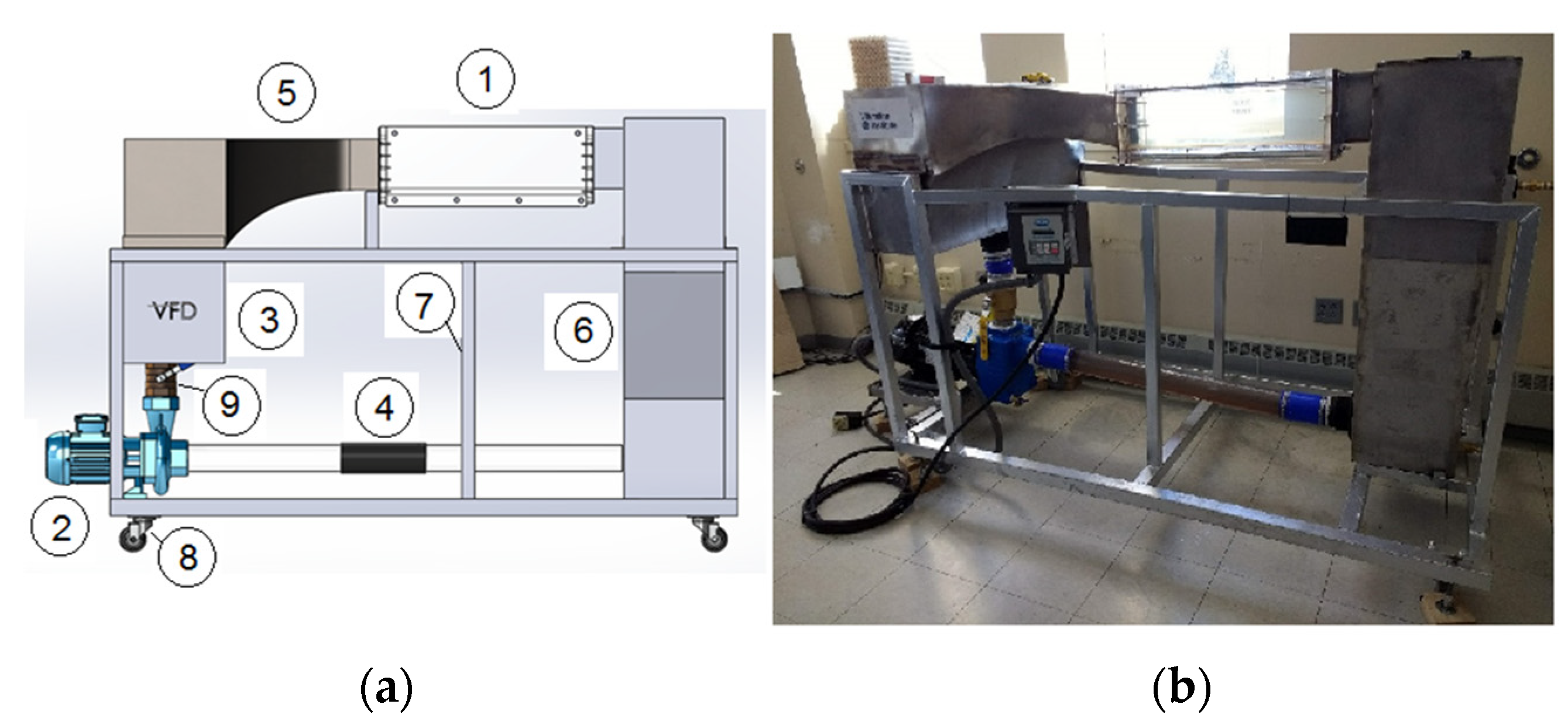
Structural analysis is paramount to determine the integrity of the flow tank and its supporting frame. Figure 2 panel (a) shows the final Computer Aided Design (CAD) drawing prepared by students and its major components. The final product of the water flow tank is shown on panel (b). The final total length of the water tank system is 2.51 m, which includes the 75 cm long observation chamber (1) and inlet manifold into the observation chamber (5) with enough entry length. In the discussion below, only the structural analysis of the supporting frame is presented.

The material chosen for the supporting frame is ASTM A513, which has a yield strength of 220.6 MPa (32,000 psi). Considering a safety factor of 1.3, the maximum yield strength for the system is ${\sigma }_y$= 169.72 MPa (24,615 psi). The beam profile used is $5.08\times 5.08$ cm² hollow square tubing with a thickness of 2.11 mm. The static analysis involves calculations of dead loads acting on the system, which includes the weight of the water and the tank.

Table 5. The table shows main loads to be considered in the design of the supporting frame.

Components	Weight (kg)	Description
Water	362.87	Total weight of water at full capacity
Observation chamber	11.16	This section is made out of acrylic
Pump	43.54	Self-priming centrifugal pump
Piping	4.72	Total weight of steel channels
Manifolds	29	Inlet and outlet chambers, made out of stainless steel
Steel strucure	4.99	Constructed out of 2 × 2 square tubings
Total dead load	456.28

lists all possible static load items and its estimated amount. The list was prepared by students as part of the full static and dynamic structural analysis of the supporting frame. Several possible designs were analyzed and results from one design is presented here.

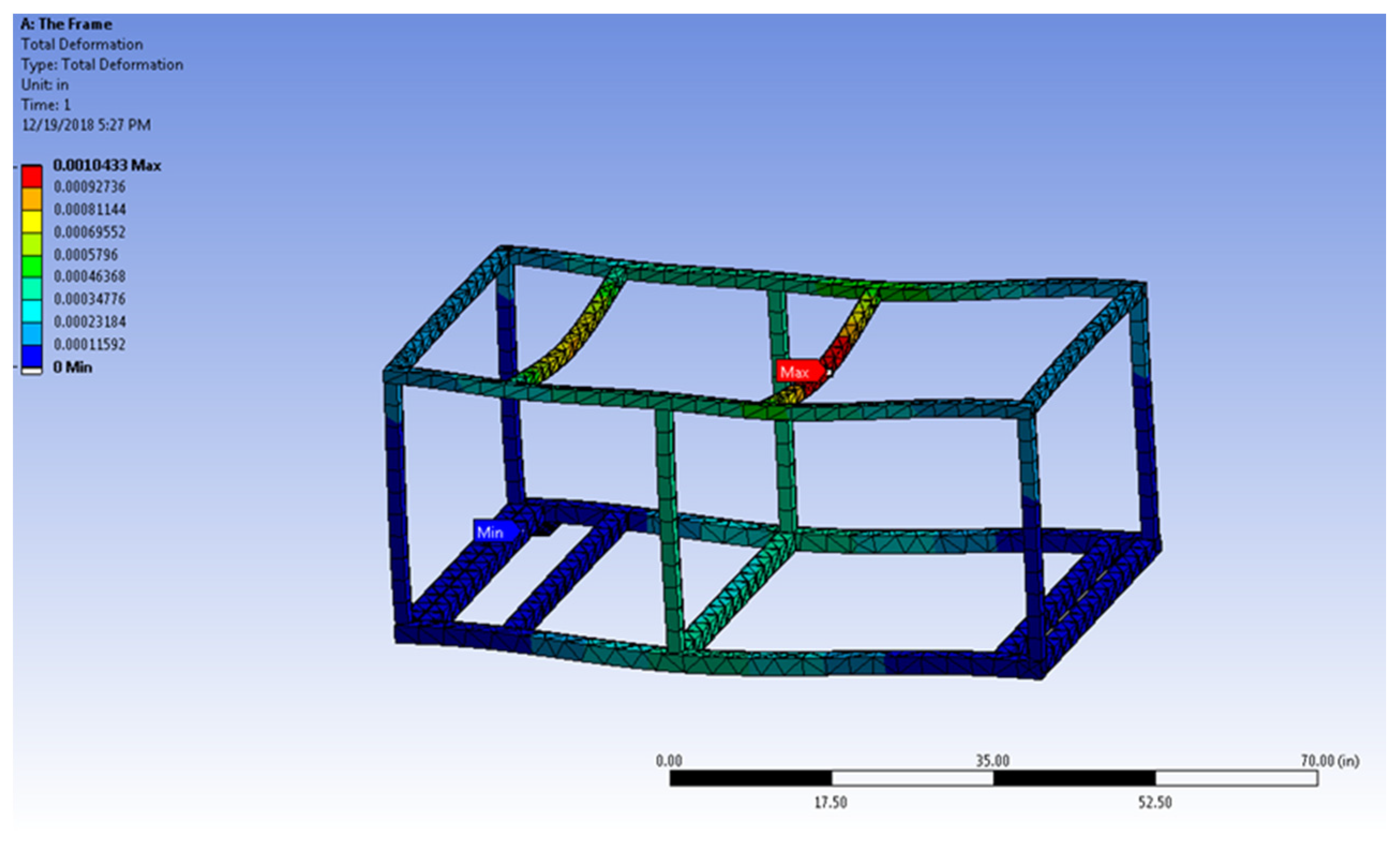
The maximum deflection of 0.0254 mm was discovered on one of the cross beams directly supporting the observation chamber. This value is considered very minimal, and it indicates that the selected channel is sufficiently strong. In this model, the frame is assumed to be supported by pins on its four bottom corners. Static loads, representing items listed in the Table 5 are applied as point loads on several locations on top beams. The water weight is distributed throughout several points on the frame. Figure 3 displays the deformation of the frame in the full 3D static analysis. As is expected, the bottom beams show minimum deformation due to the supports, while the top beams show large deformation due to the application of load.

Additionally, a dynamic modal analysis was performed using ANSYS (ANSYS Inc., Canonsburg, PA, USA) to check the mode shapes and natural frequencies of the supporting system. Outcomes from the modal analysis indicate possible resonance and amplification of deformation when the pump’s operating frequency is in the vicinity of the natural frequency of the support system. Due to the simple vibration load that is being considered, the modal analysis was set to find only the first six (6) natural frequencies. The resulting natural frequencies of the frame are presented in

Table 6. The first six natural frequencies of the supporting frames are listed in this table, along with the maximum deformation associated with the harmonic analysis.

Modes	1	2	3	4	5	6
Freq. (Hz)	23.53	36.21	39.28	70.91	73.18	86.59
Max $\delta$(mm)	2.108	2.489	2.108	2.007	5.512	2.108

. These natural frequencies were used in harmonic response analysis to determine the maximum deflection of the frame. The maximum deformation of 5.51 mm occurs for Mode 5 corresponding to the frequency of 73 Hz. Other frequencies result in maximum deformation of less than 2.54 mm. The first three (3) modes correspond to the operating frequencies of the pump of 0 to 60 Hz. Nevertheless, due to the rigidity of the structure, the amplification was found to be very minimal. The outcome suggests that the structure and material selection for this flow tank is sufficiently strong to sustain the vibration load by the pump. The study also shows that only the first 3 (or at most 4) modes need to be considered as the maximum operating frequency of the pump is only 60 Hz. Table 6 shows the six (6) first natural frequencies of the supporting frame. The maximum deformation from the harmonic analysis, based on the given static load, is also shown in this table. A maximum deformation of 5.08 mm can potentially occur for Mode 5, corresponding to ~73 Hz. Other modes show maximum deformation of less than 2.54 mm.

The first, second, and third modes represent predominantly lateral deformation of the top beams due to the rigid support of the bottom beam. The lateral deformation can occur harmoniously between the parallel top beams (Modes 1 and 3), but it can also occur non-harmoniously as in Mode 2. Mode 3 shows lateral deformation in the long direction of the frame. While the dynamic analysis shows sufficient stiffness and unlikeliness for large amplification, rubber footings were placed underneath the pump’s platform to damp the vibration.

4. Computational Fluid Dynamics

Computational fluid dynamics (CFD) analysis suggests useful information for the design of various channels of the flume. Nevertheless, the CFD simulation and analysis provide hands-on exercise materials that allow students to better understand the dynamics of flow phenomena through visualization and parametric studies [48]. Possible analysis to be performed ranges from two-dimensional to full three-dimensional study of either unsteady or steady water flow. Examples of topics to be studied include studying the flow characteristics in the observation chamber, pressure losses across the flume, undesired circulation zones, areas of turbulence, extreme stresses caused by fluid flow, etc. The computation domains of such studies can be either developed from scratch or imported from the structural mechanics CAD designs. In this section, results from a full 3D steady state analysis of water flows in a semi-loop model of the tank are briefly presented. The study is performed using the commercial package COMSOL Multiphysics 5.5 with CFD module (COMSOL Inc., Burlington, MA, USA). Most of the computations are performed using HP ProBook 640 G2 Notebook PC (Hewlett-Packard Company, Palo Alto, CA, USA). operated using 64-bit Windows 10 Enterprise version 1909 with a total capacity of ~465 GB. The computer has an installed RAM of 16 GB and is equipped with Intel^® Core™ i7-6600U CPU @ 2.60 GHz. One model is run using a desktop HP Compaq Elite 8300 CMT computer equipped with Intel^® Core TM i7-3770 CPU at 3.40 GHZ and 16.0 GB RAM.

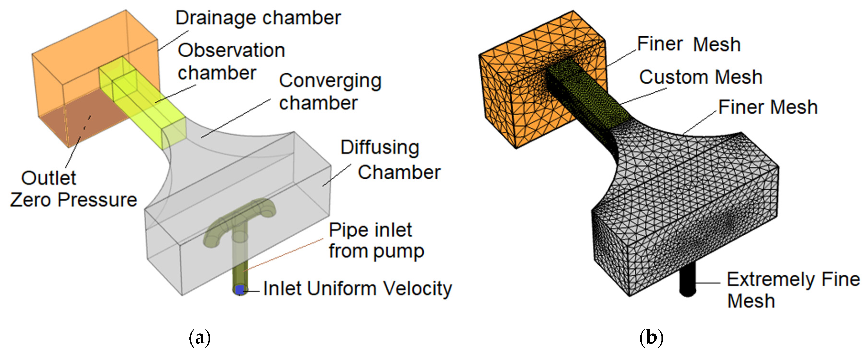
The computation domains can be differentiated into several parts, as shown in Figure 4 panel (a). The pipe inlet domain represents the vertical cylindrical thick PVC pipe channel that delivers water from the pump’s exit into the main part of the water tank. This channel is 8 cm in internal diameter and the length is 40 cm. The pipe is extended into the diffusing chamber before it splits into two horizontal branches with the same internal diameter. The resulting T-pipe allows the water to be distributed in the diffusing chamber. The T-pipe also prevents the water to “shoot up” and put high pressure on the ceiling of the diffusing chamber. The next important domain is the converging chamber that functions to collect the water and channel it into the observation chamber. A flow straightener could be included in the converging section, however this part is not modeled due to its large amount of mesh. This simplification is justified by the computation results that indicate straight uniform flow in the observation chamber (Figure 6). The observation chamber is a 60 cm long prismatic pipe with a square cross section of 15 × 15 cm². At the end of the chamber, the water is collected in a rectangular drainage tank of $60\times 30\times 40 {\mathrm{cm}}^3$. The CFD model does not include a horizontal transparent plastic pipe that returns the water back from the drainage chamber into the centrifugal pump.

Several simplifications are implemented in the CFD model. For instance, the actual drainage chamber is converging downward, but in the model only the top 40 cm section is included. It is assumed that the inclusion of this part is sufficient to recreate necessary backflow effects that occur in the observation chamber. The converging chamber attached to the distal face of the observation chamber is made to be plain horizontal, parallel to the observation chamber. The actual configuration of this curved chamber includes a slight decline in the vertical direction into the entrance of the observation chamber. Lastly, in the CFD, the observation chamber is assumed to be a closed rectangular pipe. The actual observation chamber is open on its top side to allow direct access to the water.

The inlet boundary condition is located at the free end of the inlet pipe that represents the conduit between the centrifugal pump and water tank body. Not knowing the exact velocity profile produced by the centrifugal pump, a uniformly distributed velocity profile is assumed at the inlet. The exit boundary condition is located at the bottom of the drainage chamber and a zero-pressure outlet is assumed here. The actual pressure level required by the centrifugal pump to produce the flow can be obtained by adding known hydrostatic and dynamic pressures occurred at the exit level. The internal wall is assigned to the wall of the T-pipe domain, as this pipe is located inside the diffusion chamber. The physical T-pipe has a non-zero pipe thickness that has been ignored in this CFD modeling. This important feature certainly leads to a convenience and efficient mesh generation. The remaining walls are assumed to have zero velocity. Figure 4 shows the complete model, domains, boundary conditions, and partial mesh generation that results in non-uniform mesh size throughout the domains.

CFD analysis requires a delicate balance between demands for accuracy of the outcomes versus the computational cost that are the direct results of both mesh generation and complexity of the selected flow model.

Table 7. This table lists CFD models used in this project and their associated number of elements and computation times. Only models A1 and A2 are executed using Laminar fluid model. All other models are executed using Turbulent model—RANS K-$\epsilon$ . All models are run in the HP ProBook, except Model D.

Model #	Mesh Method	Fluid Model	Number of Elements	Computation Time (s)
A1	Partial Refinement	Laminar	91,162	3630
A2	Partial Refinement	Laminar	289,796	21,787
B1	Global Extremely Coarse	Turbulent	21,011	6760
B2	Global Extra Coarse	Turbulent	43,753	17,861
B3	Global Coarser Mesh	Turbulent	76,983	34,030
B4	Global Normal Mesh	Turbulent	414,735	286,538
B5	Global Fine Mesh	Turbulent	9,797,088	Failed to converge
C	Partial Refinement	Turbulent	113,624	25,626
D	Partial Refinement	Turbulent	160,774	20,680
E	Partial Refinement	Turbulent	160,378	35,046
F	Partial Refinement	Turbulent	355,730	145,860

lists CFD models studied in this work and their mesh generation scenarios. Models As and Bs are all meshed using “Global Mesh” method, where the same mesh size or scheme is applied uniformly on all domains of the model. However, models As are computed by means of “Laminar” flow model, while models Bs are executed using “Turbulent” flow model. The C, D, E, and F models are discretized using “Partial Refinement” method and are executed using “Turbulent” flow model. Effects of the two flow models will be explained later in this section. All models are computed using the HP ProBook laptop, except model D that is executed using the desktop computer. The Global Mesh method is straightforward, but for three-dimensional models this method may result in astronomical element numbers and computation time with possible less-than-sufficient accuracy at places of interest. In the current work, we later show that partial mesh refinement on places of interest should be practiced as a choice of practice in CFD modeling, particularly for three-dimensional modeling. In our work, the “Extremely Coarse” mesh option of COMSOL Multiphysics (COMSOL Inc., Burlington, MA, USA) for our model results in 21,011 elements. Increasing the accuracy by selecting the “Normal” mesh generation option multiplies the element number to 414,735 elements, almost 20 times more than “Extremely Coarse” option. However, the computational time needed to run the model using turbulence k-$\epsilon$ scheme is multiplied from 6760 s to almost 286,538 s, 40 times longer. The partial refinement mesh generation, used for models C, D, E, and F, is performed by selecting domains or regions of interest (ROI) to be discretized finer than other domains. Here, the observation chamber, T-pipe, and inlet pipe are selected as the ROI so that the velocity profiles and other important aspects in the region can be studied more accurately. This method aims to reduce the amount of mesh and computational time, and to avoid unnecessary data collection in non-ROI parts such as the diffusing chamber, drainage chamber, and converging chamber. The Partial Refinement method certainly opens numerous possible mesh arrangements. To limit the study, we focus on mesh refinement of the ROI only. The refinement of the observation chamber sub domain will enhance accuracy of the velocity profiles in the region needed for possible two-dimensional modeling. On the other hand, the refinement of the inlet pipe and the T-pipe is expected to give accurate information on the amount of pump pressure needed in the design. These three domains will be refined using “Extremely Fine” mesh or customized mesh, while the remaining body will be meshed using either “Normal” of “Finer” scheme. For Model C, the ROI are meshed using “Extremely Fine”, while the remaining domains are meshed using “Normal”. For Models D and E, the mesh for the test chamber domain of Model C is further refined by reducing the “maximum element size” from 0.0318 to 0.015 m. Model D is the only model that is computed using the HP desktop computer. It should be noted that the “Normal” size used in the non-ROI domains of models C, D, and E employs “maximum element size” that is about triple than that of the “Normal” size used in Model B4 with global mesh method. Consequently, although the ROI domains of Models C, D, and E, are finely meshed, the total number of elements of these models are less than that of Model B4. The difference in the “maximum element size” is due to the different “Calibration” option offered by COMSOL (COMSOL Inc., Burlington, MA, USA). The mesh configuration for Model F is the finest among models with partial refinement mesh. Here, the mesh configuration of the ROI used in Model D is maintained, but the remaining domains are meshed using “Finer” mesh. This refinement results in 355,730 elements, and the computation time is 145,860 s, only half of the time needed by model B4.

Shown in Figure 4 panel (b), results of Partial Refinement strategy where high mesh density (“Extremely fine mesh”) is applied on the observation chamber, pipe inlet, and T-junction domains. The remaining domains are discretized using “Finer” mesh. The minimum and maximum element sizes employed in the observation chamber are 5 mm and 15 mm, respectively. The application would result in at least 10 computation nodes across the 15 cm wide observation chamber, which should be enough for accuracy.

The volumetric flowrate ($Q$) and mean velocity ($\overline{V}$) in the observation chamber in the inlet pipe and observation chamber will be used to measure the accuracy of the solution. The volumetric flowrate across planes perpendicular to the long direction of the observation chamber must equal to that of the inlet. This flowrate can be obtained from the uniform inlet velocity $V_{in}$ provided at the pipe inlet; $Q=V_{in}\frac{\pi }{4} D^2$, where $D$ is the pipe diameter. The mean velocity in the observation chamber can be easily estimated using $\overline{V}=\frac{Q}{A_{ch}}$, where the cross-section area of the chamber is known as $A_{ch}={0.15}^2=0.0225 {\mathrm{m}}^2$. As the outlet at the base of the drainage chamber is assumed to have a pressure drop, the flowrate at this location should also be verified.

Second only to the mesh generation, the selection of appropriate physical modeling of the fluid is the most crucial aspect of CFD modeling. The selection between Laminar and Turbulent models is often determined by Reynolds numbers involved in the problem. The laminar threshold for fully developed flow in long pipe with circular cross sections is typically around 2300, while for an open channel flow is 500. Students have to understand that the change from laminar to turbulent flow is a gradual transition, and therefore it is not practical to point out a single number to differentiate the two regimes. As pointed out by Lowe, the confusion over the critical Reynolds number is not new in the Fluid Mechanics community [49]. Nevertheless, smaller Reynolds numbers should be treated as turbulent when the complex geometry of the domains include circulation zones that are best captured using turbulent models. In the current water tank design, the maximum expected mean velocity occurring in the 15 × 15 cm square observation chamber is 60 cm per second, which results in the Reynolds number of 90,000, which puts the model under turbulent category. A long list of turbulent models is available in COMSOL Multiphysics software (COMSOL Inc., Burlington, MA, USA). For this project, we selected the standard k-$\epsilon$ model to serve our purpose. This suggested model is selected due to its popularity for industrial applications, easy convergence, and low memory requirement [50]. Alternatively, the analysis on such water flume can be performed using k-$\omega$ SST model [51]. However, a comparison study performed on a water flume with 5 m wide and 17 m long test section suggest that the outcomes from the two different Turbulent models do not show significant differences [52]. Heyrani et al. compare the performance of seven (7) turbulent models used in steady state modeling of a venturi flume. It was discovered that the k-$\epsilon$ model performs slightly better than the k-$\omega$ SST model [53].

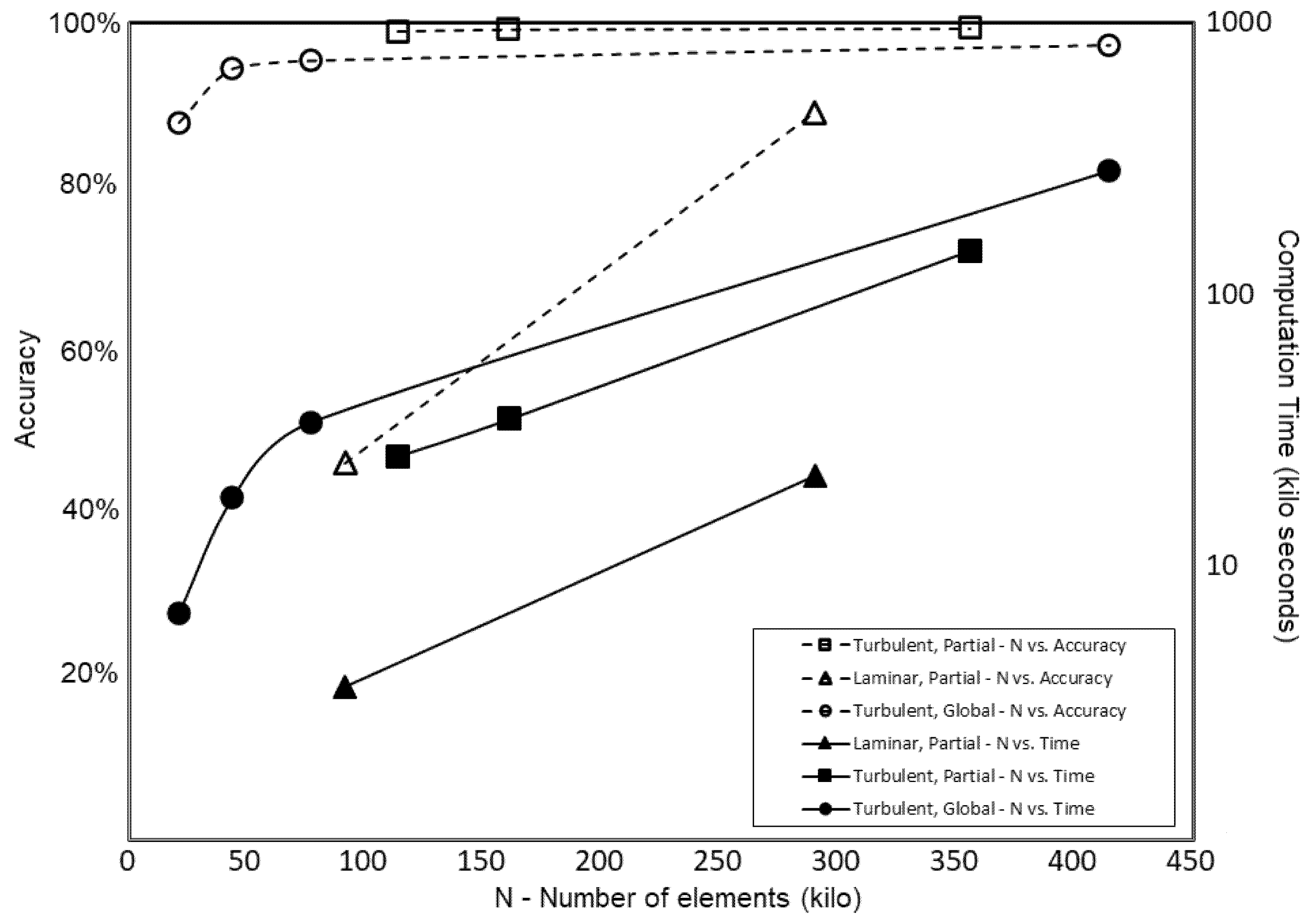
Figure 5 shows the accuracy and computation times that are plotted against the mesh number for different models. The graph shows that Turbulent model with Partial Refinement (rectangular markers) produces the best accuracy among the three models (Laminar model with Partial Refinement, Turbulent model with Global Mesh, and Turbulent model with Partial Refinement). Moreover, its computing time is less than the Turbulent model with Global Mesh (circular markers). The computing time of the Laminar model with Partial Refinement (triangular marker) is the lowest, but the accuracy is also very low. The laminar model should only be used to make sure that the CFD model can be properly executed. High accuracy can be easily achieved by the Turbulent model with Partial Refinement, even with a low amount of mesh.

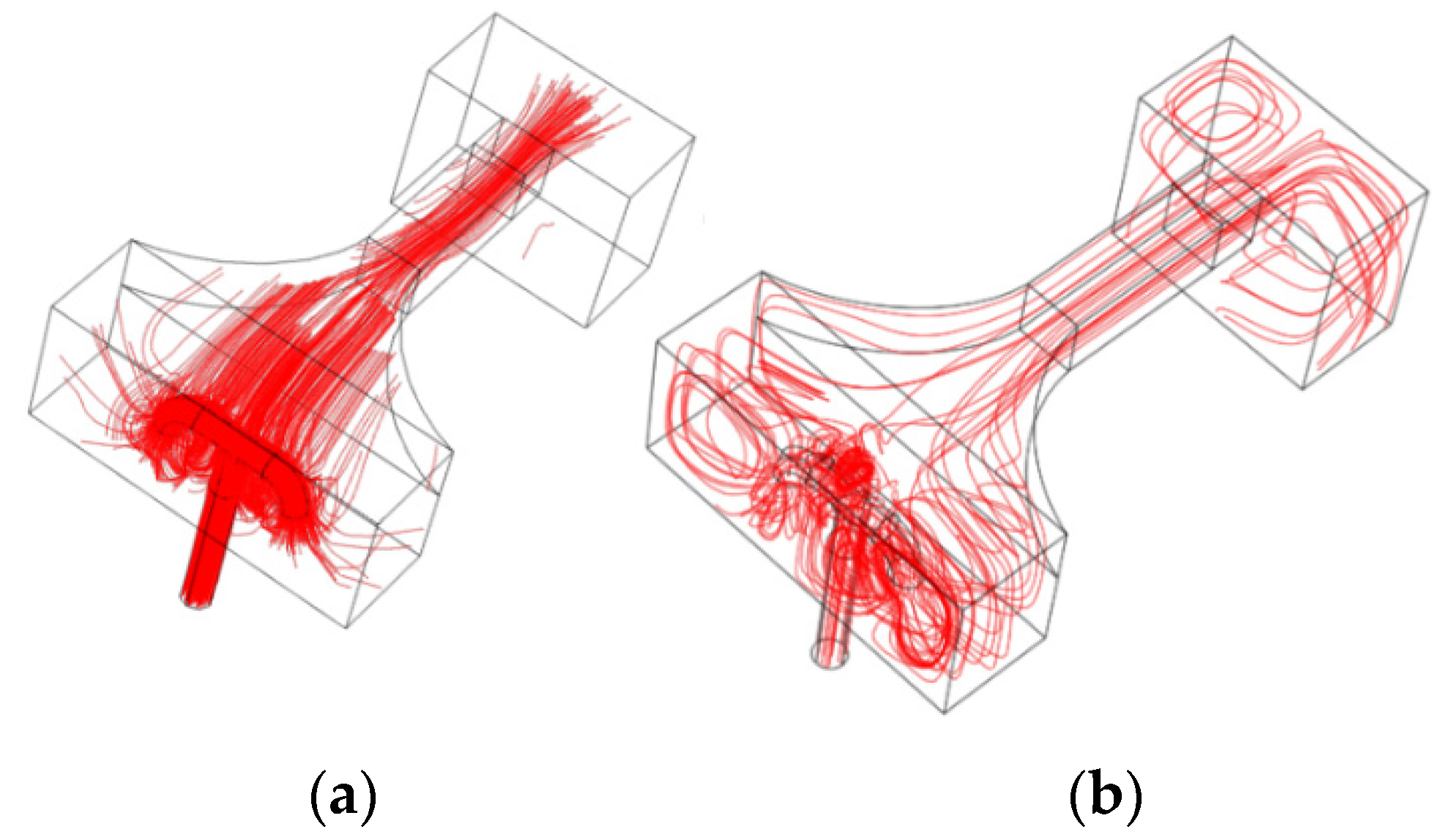
Streamlines in the water tank when the mean inlet flow is 3 m/s are shown in Figure 6. The streamlines are obtained using “standard point controlled” method and using “Number of Points” entry of 80 points. The streamlines on the left and right are obtained when the computation modules used are Laminar model and Turbulent k-$\epsilon$ model, respectively. The streamlines from the Laminar model are parallel and straight in the observation chamber, but they are clearly absent from the circular flows in the drainage chamber, as well as in the diverging chambers that are demonstrated by the Turbulent model.

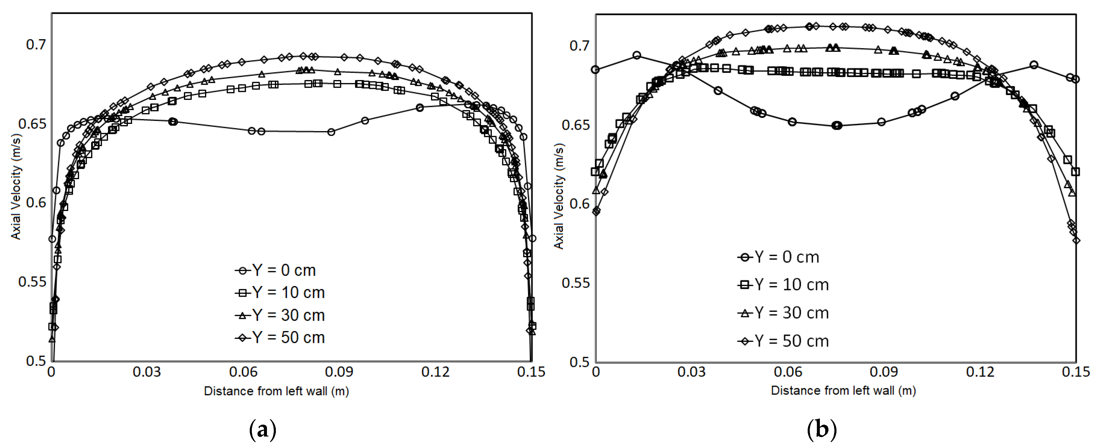
Observing the axial velocity profiles along the observation chamber, the Laminar model shows reasonable parabolic shapes (data are not shown here), however the amount of flow rate and mean velocity show deviation from the correct values. The profile of axial velocity along the observation chamber obtained from the Turbulent models are depicted in Figure 7. Each velocity profile is obtained at the same horizontal mid-section of the observation chamber, but at different distances “Y” from the starting of the chamber (taken as the interface between the converging chamber and observation chamber). The development of the velocity profile can be observed in this figure as the profile changes into a more parabolic shape as the Y is increasing. The velocity profiles demonstrate the typical characteristic of turbulent profile consisting of a turbulent core in the middle and laminar sublayer near the wall [45]. Note, however, that for the Model B4 (global mesh), the laminar sublayer is pronounced, while for Model F (partial refinement), it is very difficult to observe due to its small thickness. The accuracy of Model F in predicting the expected flowrate and mean velocity however is higher than that of Model B.

The velocity map and streamlines, viewed from the top of the flume, can be seen in Figure 8. The flow direction goes from top to bottom (diffusing chamber to the drainage chamber). Panel (a) on the left shows the velocity map of laminar model, while panels (b) and (c) are from the turbulent model, but with different mesh schemes. All models present reasonable straight parallel streamlines in the observation chamber. The Laminar model shows gradual increase in speed as it enters the observation chamber, as can be observed from the changing color. On the contrary, the Turbulent models both show consistent average velocity along the observation chamber. The Laminar model fails to produce the twin circulation zones that occur in the drainage chamber. These circulation zones are physically observed during real experimentation. The two Turbulent models clearly show these circulation zones with slight difference. The circulation zones by the Model B4 (Figure 8 panel (b)) are shown to be less chaotic than that of Model F (Figure 8 panel (c)).

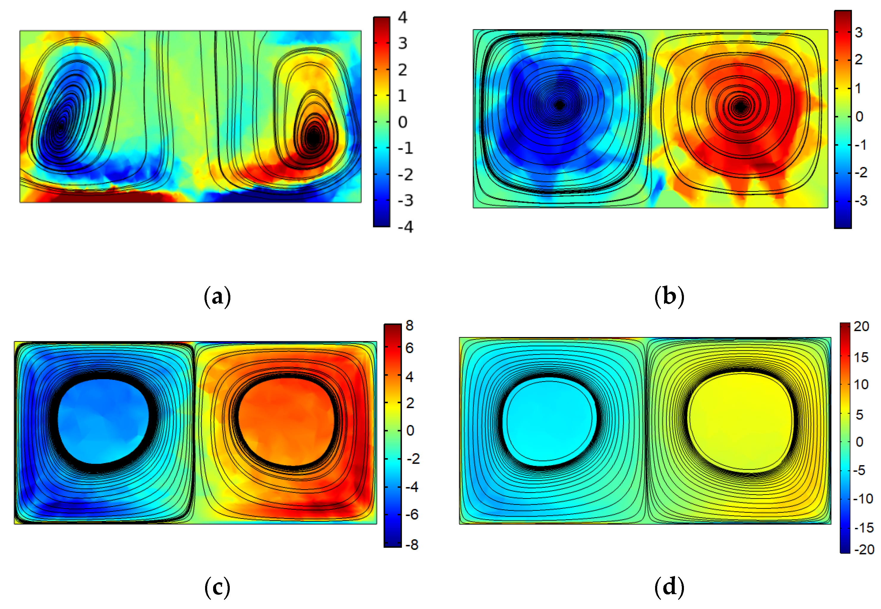
Vorticity is a local measure of the rotational motion of fluid particle relative to its own centroid, while the circulation can be considered as the measure of the rotational motion in global sense, relative to a distance reference point. After passing the observation chamber, water enters a short drainage chamber that is three times wider than the observation chamber but much deeper in the vertical sense. Here, due to the high speed in the observation chamber, the water shoots into the back wall of the chamber, but it also starts to fall due to the gravity. Hence, the stream splits into a pair of almost identical spiraling flows downward. Shown in Figure 9 are streamlines projected on a two-dimensional plane cut across approximately the middle height of the drainage chamber. On each panel, the streamlines demonstrate a pair of spiraling circles running in opposite directions. Note that the flow is coming from the observation chamber located, according to these pictures, relatively above the rectangular areas shown in the panels. The color map describes local vorticity values, and the scales indicate that, on average, the two pairs have a similar amount but in opposite directions. In this figure, each panel represents a circulation zone in the chamber from the same Reynolds numbers, around 72 K (uniform inlet velocity of 3 m/s), but each is computed using different mesh density and element types used in the drainage chamber domain. On panel (a), the fluid model is laminar, and the elements used in the drainage chamber is tetrahedral. On panels (b), (c), and (d), the k-$\epsilon$ Turbulent model is used, but the number of elements used (only in the drainage chamber) are 5498, 14,681, and 61,052, respectively. On panel (b), only tetrahedral elements are used, but various elements are used for results shown in panels (c) and (d). It can be seen that the utilization of various elements results in smooth vorticity map and streamlines that are less discrete. The symmetry of the circular flow is captured when the mesh density is very high but, generally, panel (c) shows that essential flow structure is sufficiently captured. The maximum and minimum values on the scales indicate the amount of vorticity details that can be captured by the respected mesh density. On panels (b), (c), and (d), while the maximum and minimum vorticity are different, the average values inside and around the cores of the circulation area is around 4 to 5. On panel (c) and (d), zones with large vorticity up to 20/s can be captured, but these areas are concentrated near the walls. As is expected, the large vorticity occurs near the walls where large shear strain is expected to occur. On panel (a), the Laminar model results in a pair of seemingly symmetric circulation zones. The zones, however, appear to be shifted to the side walls. Moreover, the vorticity map shows some level of local spins, but the distribution is different from that shown in other panels. The laminar model certainly has failed to produce the desired outcomes, despite of the high mesh density that has been employed.

5. Fabrication and Manufacturing

Welding was the most challenging process of the manufacturing activity in this project. All fabrication (cutting, folding, welding, assembly, etc.) had to be performed mostly off-site at a private workshop due to the space limitation for hot works in our campus. Particularly, the welding of individual manifold was the primary challenge. The inlet and outlet manifolds needed to be designed, cut, welded, and assembled without the benefit of a fully equipped fabrication facility. Furthermore, the limitations of the available workshop dictated that tolerances could be held only down to ¼” (~6.35 mm) for most features of size and ½” (~12.7 mm) for some larger features. The choice of 18 GA (0.049” or 1.27-mm) Austenitic Stainless Steel for the manifolds dictated that TIG (Tungsten static electrode Inert Gas shielded) welding was necessary to accomplish production. Alternative processes were ruled out for manifold production due to heat transfer concerns that would lead to excessive warpage of the fabricated sheet metal structures. Additional requirements of the design included the need for flush weld joints which would be less easily accomplished than other welding processes. Shown in Figure 10 one of the completed holding tanks (left) prior to being assembled with the inlet manifold (top right). The student who performed the welding used many cardboard templates (such as the one shown on panel (a) of Figure 10) to determine the cutting of the steel plate.

MIG (Metal wire feed electrode Inert Gas shielded) welding was chosen for frame production. Mild Steel Square Tube with 1/16” wall thickness (~1.59 mm) was chosen for the frame and could withstand MIG welding with minimal concerns for warpage. The design did not require the welded joints to be flush with the welded materials. The steel square tubes that were welded together required a coat of rust protective paint due to the material properties that would cause rusting. A Miller Multi-Matic 220 multi-process welder (Miller Electric Manufacturing Co., Appleton, WI, USA) was used for all welding processes, selected due to its versatility of process selection and advanced user interface and arc control systems. The frame had undergone minor modifications from the original design to acclimate for the weight of the pump, transportation, and vibrations that would pass through the system. Jack screws, similar to stands, allowed the system to elevate off the wheels to limit vibration through the floor, level the entire system and to relieve stress from the wheels, as their specifications stated that they would only withstand 544.31 kg. The frame that the pump was set onto had its own set of jack screws that allowed it to be lifted off the frame for the rubber insulators to absorb vibrations produced by the pump. The 15 × 15 × 60 cm³ observation chamber was made of 0.635 cm thick transparent plexiglass. The corners are secured using both glue and bolts. To prevent leaking, rubber gasket is applied throughout. Finally, several holes are drilled on the upper edge of the chamber wall (not shown in the figure) to allow experiment platform to be secured onto.

6. Experiment Results and Discussion

The following experiments were conducted using the water tank after its fully built to test its capability:

• Velocity Measurement of flow in the observation chamber;
• Tests on flow straightener designs;
• Flow visualization using dye;
• Measurements of drags.

6.1. Velocity Measurement of Flow in the Observation Chamber

The speed of the water flow can be controlled by adjusting the rotational speed or frequency of the pump’s propeller using the programmable speed controller. In the first experiment, we wish to establish the relationship between the frequency of the propeller and the resulting water velocity in the observation chamber. The average velocity in the observation chamber is measured using a flow meter by Vernier (Vernier, Beaverton, OR, USA) (product number FLO-BTA) shown in Figure 11 panel (a). The sensor is designed for external flow measurement such as flow in open channels and rivers. The measurement range of this affordable sensor is up to 4 m/s, with a typical resolution of $\pm 1.2$ mm/s, and an accuracy of about 1 percent. A data acquisition card, LabQuest Mini, also by Vernier (product number LQ-MINI), is used to collect the data and transfer the data to a laptop through a USB cable. The dynamic data can be displayed by Graphical Analysis GUI software available for free by Vernier. The data can be exported to either Excel, Matlab, or Phyton, for further analysis and post processing. Typical data sampling in our experiment is 1 Hz.

During one set of data collection, we seek to check the speed variability across the chamber’s depth. Here, we perform the flow measurement by placing the sensor’s propeller near (about 3 cm above) the chamber’s floor and approximately at mid-height above the chamber’s floor. The data collection for each trial was done at least for 40 s. On each trial, the frequency of the pump is increased from 10 Hz to 60 Hz using intervals of 10 Hz. This data collection results in insignificant variability of the time-averaged speed between the two locations. Examples of data collected over a period of 120 s for pump frequencies of 40 Hz and 50 Hz are shown in Figure 11 panel (b). The transient regime for about 25 s at the beginning of data collection can be easily identified in both data. The steady state regime maintains a constant average speed and indicates small fluctuations. Data with solid labels are taken for measurement at “Bottom”, while data with open labels are from “Middle”. Data indicate that the placement of samples in between these two locations would result in more-or-less identical outcomes.

6.2. Tests on Flow Straightener Designs

The second set of experiments involved velocity measurement in the presence of a flow straightener. The flow straightener functions to dissipate the turbulence water flowing into the observation chamber. The three (3) designs by students are shown in Figure 12; Models 1, 2, and 3 displayed in panels (a), (b), and (c), respectively. The cross section of all the models is 15 × 15 cm. Model 1 was constructed by PVC tubes of the same diameter (12.7 mm) cut at the same length (~10 cm) that are glued along its long sides. These cut pipes were then arranged in parallel, and bonded together on its long sides to form a channel. This model has the largest area of holes. Model 2 is a 3D-printed PLA plastic rectangular block of 15 × 15 × 5 cm³, furnished with 12-by-12 holes, each about 1.2 cm in diameter. Model 3 is a combination of parallel 0.5”-PVC (12.7 mm in diameter) pipes that are hold together using 3D-printed blocks with holes on their ends. Among the three models, Model 1 is the cheapest, but is very tedious to make, as each pipe has to be glued one by one. During the bonding process, the pipes can be placed in between two parallel walls. Model 2 is the most expensive, when the printing time is included in the calculation. While the SolidWorks (Dassault Systèmes SolidWorks, Inc., Waltham, MA, USA) CAD model for this model is easy to make, it took more than 12 h to print the model using a regular desktop 3D-printer. The thin walls separating the holes require the model to be printed with high density (high infills), and this prolongs the printing process. While involving 3D-printed blocks, Model 3 is inexpensive, as the holes on these blocks are well separated from one another, requiring less printing density compared to Model 2. Nevertheless, the arrangement of the pipes into these blocks is quite tedious. In terms of durability, it was quickly found that Model 1 disintegrated quite easily after several tests in the water. Model 2 also shows signs of plastic fibers detached from the bulk structure after several tests. Model 3 is the most durable, but its effectiveness is the lowest.

The data of flow velocity, taken when the pump’s speed is 10 Hz, versus time for different models of flow straighteners, are presented in Figure 13. The blue, red, black, and green lines indicate water velocity without flow straightener, with Model 1, with Model 2, and with Model 3, respectively. On average, the velocity data for Model 1 (red line) is very similar to the case where no flow straightener is installed (blue line). Some degree of deviation from the flow with no straightener (blue line) is reflected by data using Model 2. Compared to other models, Model 3 shows the largest deviation from the flow with no flow straightener (blue line). Clearly, the Model 1 produces the least flow disturbance in terms of time-averaged velocity outcome. The expected outcomes can be attributed to the difference in the cross-section areas of the holes of each model. The largest area of holes for Model 1 is contributed by the holes by the pipes and the holes in between these pipes. Nevertheless, the Model 2 can be seen to produce a more stable velocity (black line) across the time compared to Model 1 and Model 3.

Time-averaged (over the steady state period) water flow velocity obtained from the flow meter for various pump’s frequencies are presented in Figure 13. The data points are labeled using white circles (no flow straightener), white square (Model 1 of flow straightener), and white triangle (Model 2 of flow straightener). A linear relationship of

$$\overline{V}=0.014\times Fr-0.042 \left(R^2=0.9999\right)$$

(4)

was discovered for data obtained without the flow straightener. Here, $\overline{V} \left(\mathrm{m}/\mathrm{s}\right)$ and $Fr \left(Hz\right)$ are the mean velocity and pump’s frequency, respectively. The non-zero intercept suggests the minimum frequency (associated with a minimum water velocity) needed to turn the propeller of the flow meter of about 3 Hz. The known linear relation between the pump’s frequency and average velocity establishes the formulation of $\overline{V} vs. F.$ for future experimentation. Velocity data obtained using the flow straightener Model 1 shows similarity to the data obtained without the flow straightener. On the other hand, Model 2 produces velocity data that deviates at high pump’s frequency. The linear relationship is also quantified as $\overline{V}=0.0166\times Fr-0.0663 \left(R^2=0.9951\right)$.

On a separate, simple experiment, two students measured the water velocity by means of a Lagrangian approach. Here, the time needed by a ~1 × 1 × 2 cm³ cork to travel for 50 cm is measured using a manual stopwatch. This measurement results in smaller velocity compared to ones measured using the propeller. These Lagrangian velocities are displayed in Figure 14 using dark cross legends. The lower estimation can be attributed to the drag produced by the weight of the cork, as well as accuracy of the manual data collection. Nevertheless, the manual measurement using cork provides a simple and quick validation of the Eulerian method employed in the automatic measurement using digital flow meter.

6.3. Flow Visualization Using Dye

The effects of placing the flow straightener in the water stream was examined by means of dye injection. While this method is simple and affordable, students performing the tasks can learn valuable lessons. For example, students realize that the fluid density had to be carefully chosen, as a fluid that was too light would rise to the top (float) and the fluid mixture was too dense then it would sink to the bottom. The fluid was also mixed with food coloring to make it easier to observe. After running several tests using hand soap, oil, sugar, and honey, it was concluded that honey diluted with a small amount of water gave the best results. These tests were run by using a syringe with the mixed fluid. Figure 15 shows the difference in flow behavior through the utilization of injected dye. The left picture (panel (a)) shows the flow turbulence when there is no flow straightener inserted in the chamber. Panels (b) and (c) show the resulting flow behavior when Model 2 is used. Here, the flow is almost straight and uniform with minimum turbulence characteristic.

6.4. Measurements of Drags

Objects exposed to fluid flow experienced both drag and lift forces. Being able to demonstrate this phenomenon for objects in the water flow is one important objective of the water flume project. Experimentation on drag reported below was performed by students in Thermal Fluid Lab course on Fall 2019. The drag force acting on objects, such as long prismatic cylinders and bars, is registered using a force sensor from Vernier (Go Direct ^® Force Sensor—GDX-FOR) that uses strain gauge to measure as small as $\pm 0.1 \mathrm{N}$ up to $\pm 50 \mathrm{N}$ of axial force, sufficient range for our fluid application. A sampling rate of 50 Hz, out of a possible maximum of 1000 Hz, is used in our application. This device can be either directly connected to a laptop using a USB cable, or wirelessly using a Bluetooth to a mobile device. The stream data can be displayed on a laptop and recorded using a software Graphical Analysis available for free from Vernier. The force sensor can also be connected to the data acquisition card by Vernier—LabQuest Mini. This allows simultaneous measurement of multiple sensors with other data such as water speed, temperature, and lift. The ~7 × 4 × 5 cm³ sensor device is placed on $~15\times 15\times 1.5 {\mathrm{cm}}^3$ (1.36 kg) aluminum sled supported by four smooth wheels (rollers) that rest on the walls of the observation chamber (Figure 16). The sled was machined to include a hollowed pin on its top to secure the force sensor. A hole was drilled at the center of the sled to allow samples to be secured using bolt and nut. The other end of the bar is free. The force registration is performed by aligning the sensor’s hook to the flow direction and securing it to a reference point fixed to the chamber’s wall. The four smooth wheels reduce the contribution friction caused by the sled’s weight and maximize the registration of the hydrodynamic drag by the sensor.

The drag measurement has been conducted for several objects: plastic cylinders, 3D-printed cylinders, solid aluminum cylinders, and square bars, as well as rotating bladeless turbine models. A preliminary attempt using a 3D-printed fixture to hold hollow plastic cylinder samples and 3D-printed samples resulted in promising data. However, it also indicated the need for rigid and sturdy support and samples that do not float. The force data is converted into Drag Coefficient, $C_D$ using the following formulation [43,44]:

$$C_D=\frac{2{\overline{F}}_D}{\rho {\overline{V}}^{2}A}$$

(5)

where ${\overline{F}}_D, \rho , \overline{V},$ and $A$ are the time-averaged drag force, water density, time-averaged water velocity, and frontal area of the cylinder sample, respectively. The frontal area only accounts for surface perpendicular to the water flow. Only data from the 16 mm diameter aluminum cylinder and square aluminum bar are presented in this report.

Shown in Figure 17 is an example of raw data of the force obtained from the force sensor for a period of 120 s when the data is taken at 50 Hz sampling frequency. The average velocity of the water flow here is about 59.4 cm per second. The oscillation of drag force is expected to be caused by the unsteadiness of the flow and the vortex shedding that occurs when fluid flow passes the object. The average force is about 0.38 N, and its standard deviation is $\pm 0.072 \mathrm{N}.$

The drag force data for each sample was collected for four different pump speeds: 0.35, 0.50, 0.60, and 0.66 m/s. All measurement was obtained when steady state had been reached. Figure 18 shows monotonic and non-linear increase in the drag forces for the samples in the range of the applied flow speed. The two samples demonstrate a very similar trend. The error bars show the standard deviation over the data population of speed and force measurement. The error percentage presented by the flow meter is less than that by the force sensors. A consistent increase in the deviation from the mean of the force data is observed when the flow speed increases. This is expected, as the force should be proportional to the square of flow speed. Data from the flow meter indicate consistent deviation throughout the range of the flow speed.

Figure 19 shows the plot of the average drag coefficients for increasing Reynolds numbers. The average ${\overline{C}}_D$ here is calculated using the time-averaged velocity and time-averaged force taken at a specific pump’s frequency. The error bars indicate the “maximum” and “minimum” values of the drag coefficients, calculated using the maximum and minimum velocity and force data reading. The large fluctuation of force data at high velocity is reflected here as large range of “maximum” and “minimum” coefficients. Nevertheless, the average drag coefficients for both cases remain relatively constant in the presented range of Reynolds numbers. The average drag coefficients, over the given Reynolds numbers, are $1.48\pm 0.25$ and $1.58\pm 0.13$ for the cylinder and square bar, respectively. The plot of $C_D$ for cylindrical bar as a function of Reynolds numbers for $0\le Re\le {10}^4$, proposed by Tang et al. [54], is also shown in this figure. The expression is stated here for clarity:

$$C_D={10}^{{\left(0.0041\times (\log \left(Re\right)\right)}^3+0.0853\times {\left(\log \left(Re\right)\right)}^2-0.65\times \log \left(Re\right)+1.05)}$$

(6)

The function is obtained by regression analysis of $C_D$ data on cylinder bars obtained from various data collection. The dash line in Figure 19 shows the constant $C_D$ number for a long cylinder that is typically published in textbooks. The presented comparison shows that the $C_D$ values obtained in our lab can be considered reasonable. For $C_D$ of the cylinder bar, the deviation from both published $C_D$s is large when the Reynolds number is low, but the error is minimized as the Reynolds number increases. The outcome certainly warrants further refinement of the experiment apparatus and more data collection at various Reynolds numbers.

Alternatively, the drag coefficients can be obtained by first plotting the drag force data against the square of the time-averaged speed, as shown in Figure 20. Using standard linear regression analysis, the linear relationship between $F_D$ and ${\overline{V}}^2$ can be obtained. For the presented samples, the following relations are obtained ${\overline{F}}_D=1.1623 {\overline{V}}^2$ and ${\overline{F}}_D=1.3449 {\overline{V}}^2$ for the cylinder bar and square bar samples, respectively. The high $R^2$ values for the two samples indicate a strong fit in the regression process. It also indicates that the linear relation is appropriate, as the $C_D$ is expected to be constant in the applied range of Reynolds numbers. Note that the zero intercept in this case is not automatic, and it must be enforced as the zero force should be correlated with zero velocity. Eventually, the drag coefficients can be calculated from the gradients of the lines using the following formulation, which can be derived from (4)

$${\widehat{C}}_D=\frac{2 K}{\rho A}$$

(7)

where $K$ is the gradient of the linear relationship between ${\overline{F}}_D$ and ${\overline{V}}^2$. The coefficients found using this method are very similar to the average coefficients, however this method results in coefficients that are closer to the known values from textbooks [43,44,45].

Presented in

Table 8. List of the $C_D$ values obtained in our experiments compared to that presented in textbooks. The 2D and 3D refer to the two-dimensional and three-dimensional assumptions of the immersed bodies. The ${\overline{C}}_D$ refers to the averaged coefficient of drag. The ${\widehat{C}}_D$ is obtained using the linear regression analysis of ${\overline{F}}_D vs. {\overline{V}}^2$.

Sample	Diameter/Side	${\overline{\mathit{C}}}_{\mathit{D}}$	${\widehat{\mathit{C}}}_{\mathit{D}}$	$\mathbf{Known}{\mathit{C}}_{\mathit{D}}\left(2\mathbf{D}\right)$ [44]	$\mathbf{Known}{\mathit{C}}_{\mathit{D}}\left(3\mathbf{D}\right)$ [44]
Cylinder	15.94 mm	$1.48\pm 0.25$	1.39	1.2	0.74–0.82
Square bar	15.93 mm	$1.58\pm 0.13$	1.61	2.1 or 2.2

is a list of the $C_D$ values obtained in our experiments compared to those presented in textbooks. The 2D and 3D refer to the two-dimensional and three-dimensional assumptions of the immersed bodies. The ${\overline{C}}_D$ refers to the averaged coefficient of drag. This ${\overline{C}}_D$ is obtained by simply taking the average of all $C_D$s calculated using different mean velocities and their corresponding drag forces. The alternative ${\widehat{C}}_D$ is obtained by first plotting the drag force versus the square of the mean velocities (${\overline{F}}_D vs. {\overline{V}}^2)$ and then computing the gradients of their linear relationship. The last column of the table shows the $C_D$ value when the cylinder is considered as a three-dimensional (3D) body. The length-to-diameter ratio of our sample is $\frac{L}{D} ~ 7$, and the corresponding $C_D$ value is in between 0.74 and 0.82 [44]. Compared to the 2D version of the known values, both methods result in drag coefficients within reasonable margin errors for the given experiment setup and range of applied Reynolds numbers ($5000\le Re\le {10}^4$). The known 2D $C_D$ is stated to be valid for ${10}^3\le Re\le {10}^4$ (laminar regime), while the 3D $C_D$ is valid for $Re\ge {10}^4$ (turbulent regime) [44].

Given the limitation of the support system and the accuracy of the sensors, the drag coefficients obtained in this experiment can be considered reasonable. The close walls presented by the observation chamber introduce effects on the vortex trail, hence the drag forces. Numerical studies at low Reynolds numbers showed that the wall increases the drag coefficient [55,56]. Experimentation at high Reynolds numbers (above 3000) on a cylinder, flat plates, and a square bar indicates the effects of walls on the pattern of the vortex-shedding [57]. The presence of the flow meter upstream of the sample, as mentioned previously, should have affected the force reading. Simultaneous flow rate reading is not necessary, as the relationship between the pump’s frequency and flow speed has been known. Alternative supporting systems for the bar, for example pin support or fixed support on both ends, should be studied in future. Lastly, the absence of flow straightener needs to be considered, as it is known to affect the flow characteristics in the observation chamber.

7. Budget

Table 9. List of major components of the flume, amount and its 2018 price. Note that the labor cost is not included here.

Item	Total Price (USD)	Percent of Total Cost (%)
3″ Self-priming centrifugal pump	1105	19.91
Programmable 3-phase AC motor speed control	723	13.03
Acrylic Sheet 0.7″ thickness	298	5.37
Stainless Steel (various thickness)	805.9	14.52
Low-carbon steel square tubes and sheets	694.5	12.51
Various hoses, pipes, and fittings	654	11.78
Various bearings and mountings	138.8	2.50
PVC pipes, fitters, and elbows	159	2.86
Welding screen	240	4.32
Argon gas supply for welding	504	9.08
Various shipping of items	228.5	4.12
Total	5551	100

shows major items purchased for the flow tank, totaling approximately USD 5550. This is slightly higher than the USD 3500 cost of a custom-made water tunnel with a 30 cm wide and 180 cm long test section reported by Darfler and Tsai [2]. Our budget matches well with a flow loop with similar scale testing chamber reported by Northern Arizona State University [58]. However, this system can only perform laminar flow due to the small pump size. The centrifugal pump, as is expected, is the most expensive item in our project. However, its cost is still less than 22% of the total budget. The cost for the speed controller is also modest. The remaining cost covers the materials, such as stainless steel plates for the tank body, an acrylic sheet for the observation chamber, various pipes and valves for connectors, and steel tubes for the supporting frames. Gas supply for the welding takes less than USD 1000. The total cost listed here does not include the labor cost for the welding, assembly, design, transportation, wiring, and painting. All price is based on 2018 market values. An up-to-date pump price may be found on the manufacturer’s website [59].

8. Conclusions

The design and manufacturing process of an educational water flume has been shown to provide a learning platform for engineering students. The project is suitable for a senior design capstone project that would take two (2) semesters to complete. The design process has provided complex hands-on exercise materials for students desiring to master engineering fundamentals and skills such as computer aided designs, computer analysis of structures and fluid flows, electrical circuits, and experimentation. The open flume can be an expensive investment, but its versatility truly provides avenues for multi-disciplinary creative research. For a small-scale water flume, the required pump is governed by the height of the observation chamber and desired flow rate for the experiments. Welding of the tank body and supporting frames take the most challenging step and must be facilitated well. Professional welding and manufacturing, when budget is allowed, should be preferred to obtain a quality product, as rusting can become imminent.

References

1. Bixler, B.; Pease, D.; Fairhurst, F. The accuracy of computational fluid dynamics analysis of the passive drag of a male swimmer. Sports Biomech. 2007, 6, 81–98. [Google Scholar] [CrossRef] [PubMed]
2. Darfler, R.C.; Tsai, W.W. Method for a Low Cost Hydrokinetic Test Platform: An Open Source Water Flume. In Proceedings of the ASEE Annual Conference and Exposition, Columbus, OH, USA, 25–28 June 2017. [Google Scholar] [CrossRef]
3. Washuta, N.J.; Howison, J.; Clark, B.L.; Imhoff IV, R.H.; Dos Reis, L. Water Tunnel Design; A Senior Capstone Project to Promote Hands-on Learning in Fluids. In Proceedings of the ASEE Annual Conference and Exposition, Salt Lake City, UT, USA, 24–27 June 2018. [Google Scholar] [CrossRef]
4. Panah, A.E.; Barakati, A. Design and Build a Water Channel for a Fluid Dynamics Lab. In Proceedings of the ASEE Annual Conference and Exposition, Columbus, OH, USA, 25–28 June 2017. [Google Scholar] [CrossRef]
5. Cohrs, M.; Ernst, W.; Vaidya, A. Potential for energy harvesting from vortex induced oscillations. Int. J. Ecol. Dev. 2013, 26, 1–9. [Google Scholar]
6. Camassa, R.; Chung, B.J.; Howard, P.; McLaughlin, R.; Vaidya, A. Vortex induced oscillations of cylinders at low and intermediate reynolds numbers. In Advances in Mathematical Fluid Mechanics—Dedicated to Giovanni Paolo Galdi on the Occasion of His 60th Birthday; Springer: Berlin/Heidelberg, Germany, 2010; pp. 135–145. [Google Scholar] [CrossRef]
7. Araneo, J.; Chung, B.J.; Cristaldi, M.; Pateras, J.; Vaidya, A.; Wulandana, R. Experimental control from wake induced autorotation with applications to energy harvesting. Int. J. Green Energy 2019, 16, 1400–1413. [Google Scholar] [CrossRef]
8. Wulandana, R.; Foote, D.; Vaidya, A.; Chung, B.J. Vortex-Induced Autorotation Potentials of Bladeless Turbine Models. Int. J. Green Energy 2021. (accepted for publication). [Google Scholar]
9. Sun, W.; Zhao, D.; Tan, T.; Yan, Z.; Guo, P.; Luo, X. Low velocity water flow energy harvesting using vortex induced vibration and galloping. Appl. Energy 2019, 251, 113392. [Google Scholar] [CrossRef]
10. Cao, D.; Ding, X.; Guo, X.; Yao, M. Design, Simulation and Experiment for a Vortex-Induced Vibration Energy Harvester for Low-Velocity Water Flow. Int. J. Precis. Eng. Manuf. Green Technol. 2020, 8, 1–14. [Google Scholar] [CrossRef]
11. Cao, D.; Ding, X.; Guo, X.; Yao, M. Improved Flow-Induced Vibration Energy Harvester by Using Magnetic Force: An Experimental Study. Int. J. Precis. Eng. Manuf. Green Technol. 2020, 8, 879–887. [Google Scholar] [CrossRef]
12. Arionfard, H.; Nishi, Y. Experimental investigation of a drag assisted vortex-induced vibration energy converter. J. Fluids Struct. 2017, 68, 48–57. [Google Scholar] [CrossRef]
13. Fernandes, A.C.; Armandei, M. Low-head hydropower extraction based on torsional galloping. Renew. Energy 2014, 69, 447–452. [Google Scholar] [CrossRef]
14. Rostami, A.B.; Fernandes, A.C.; Bakhshandeh Rostami, A.; Fernandes, A.C.; Rostami, A.B.; Fernandes, A.C. The effect of inertia and flap on autorotation applied for hydrokinetic energy harvesting. Appl. Energy 2015, 143, 312–323. [Google Scholar] [CrossRef] [Green Version]
15. Fernandes, A.C.; Bakhshandeh Rostami, A. Hydrokinetic energy harvesting by an innovative vertical axis current turbine. Renew. Energy 2015, 81, 694–706. [Google Scholar] [CrossRef]
16. Rostami, A.B.; Fernandes, A.C. Mathematical model and stability analysis of fluttering and autorotation of an articulated plate into a flow. Commun. Nonlinear Sci. Numer. Simul. 2018, 56, 544–560. [Google Scholar] [CrossRef]
17. Raghavan, K.; Garcia, E.M.H.; Bernistas, M.M.; Ben-Simon, Y. The Vivace converter: Model tests at reynolds numbers around 100,000. J. Offshore Mech. Arct. Eng. 2009, 131, 1–13. [Google Scholar]
18. Chang, C.-C.J.; Kumar, R.A.; Bernitsas, M.M. VIV and galloping of single circular cylinder with surface roughness at 3.0× 10⁴≤ Re≤ 1.2× 10⁵. Ocean Eng. 2011, 38, 1713–1732. [Google Scholar] [CrossRef]
19. Bernitsas, M.M.; Raghavan, K.; Ben-Simon, Y.; Garcia, E. VIVACE (Vortex Induced Vibration Aquatic Clean Energy): A New Concept in Generation of Clean and Renewable Energy From Fluid Flow. ASME J. Offshore Mech. Arct. Eng. 2008, 130, 41101–41115. [Google Scholar] [CrossRef]
20. Shao, N.; Lian, J.; Liu, F.; Yan, X.; Li, P. Experimental investigation of flow induced motion and energy conversion for triangular prism. Energy 2020, 194, 116865. [Google Scholar] [CrossRef]
21. Yan, X.; Lian, J.; Liu, F.; Wang, X.; Shao, N. Hydrokinetic energy conversion of Flow-induced motion for triangular prism by varying magnetic flux density of generator. Energy Convers. Manag. 2021, 227, 113553. [Google Scholar] [CrossRef]
22. Barber, R.B.; Hill, C.S.; Babuska, P.F.; Wiebe, R.; Aliseda, A.; Motley, M.R. Flume-scale testing of an adaptive pitch marine hydrokinetic turbine. Compos. Struct. 2017, 168, 465–473. [Google Scholar] [CrossRef] [Green Version]
23. Okulov, V.L.; Naumov, I.N.; Kabardin, I.; Mikkelsen, R.; Sørensen, J.N. Experimental investigation of the wake behind a model of wind turbine in a water flume. J. Phys. Conf. Ser. 2014, 555, 012080. [Google Scholar] [CrossRef] [Green Version]
24. Talukdar, P.K.; Sardar, A.; Kulkarni, V.; Saha, U.K. Parametric analysis of model Savonius hydrokinetic turbines through experimental and computational investigations. Energy Convers. Manag. 2018, 158, 36–49. [Google Scholar] [CrossRef]
25. Sarma, N.K.; Biswas, A.; Misra, R.D. Experimental and computational evaluation of Savonius hydrokinetic turbine for low velocity condition with comparison to Savonius wind turbine at the same input power. Energy Convers. Manag. 2014, 83, 88–98. [Google Scholar] [CrossRef]
26. Kailash, G.; Eldho, T.I.; Prabhu, S.V. Performance study of modified savonius water turbine with two deflector plates. Int. J. Rotating Mach. 2012, 2012. [Google Scholar] [CrossRef] [Green Version]
27. Patel, V.; Eldho, T.I.; Prabhu, S.V. Performance enhancement of a Darrieus hydrokinetic turbine with the blocking of a specific flow region for optimum use of hydropower. Renew. Energy 2019, 135, 1144–1156. [Google Scholar] [CrossRef]
28. Kyozuka, Y.; Akira, H.; Duan, D.; Urakata, Y. An Experimental Study On the Darrieus-Savonius Turbine For the Tidal Current Power Generation. In Proceedings of the Nineteenth International Offshore and Polar Engineering Conference, Osaka, Japan, 21–26 June 2009. [Google Scholar]
29. Jahangir Alam, M.; Iqbal, M.T. Design and development of hybrid vertical axis turbine. In Proceedings of the Canadian Conference on Electrical and Computer Engineering, St. John’s, NL, Canada, 3–6 May 2009; pp. 1178–1183. [Google Scholar] [CrossRef]
30. Volpe, M.A.; Beninati, M.L.; Riley, D.R.; Krane, M.H.; Fontaine, A.A. Development of measurement methods for testing of hydrokinetic devices to evaluate the environmental effect on local substrate. In Proceedings of the OCEANS’11-MTS/IEEE Kona, Waikoloa, HI, USA, 19–22 September 2011. [Google Scholar] [CrossRef] [Green Version]
31. Zhou, T.; Endreny, T.A. Reshaping of the hyporheic zone beneath river restoration structures: Flume and hydrodynamic experiments. Water Resour. Res. 2013, 49, 5009–5020. [Google Scholar] [CrossRef]
32. Duan, G. Upgrading an Experimental Flume for Engineering Research Education. 2009. Available online: https://apps.dtic.mil/sti/citations/ADA516451 (accessed on 1 December 2020).
33. Ubing, C.; Ettema, R.; Thornton, C.I. Flume experiments on baffle-posts for retarding open channel flow. J. Hydraul. Res. 2017, 55, 430–437. [Google Scholar] [CrossRef]
34. Bong, C.H.J.; Liow, C.V. Hydraulic characteristics of flow through angled baffle-plates in an open channel. Int. J. River Basin Manag. 2020, 18, 377–382. [Google Scholar] [CrossRef]
35. Roussinova, V.; Balachandar, R. Open channel flow past a train of rib roughness. J. Turbul. 2011, 12, 1–17. [Google Scholar] [CrossRef]
36. Yiping, L.; Anim, D.O.; Wang, Y.; Tang, C.; Du, W.; Lixiao, N.; Yu, Z.; Acharya, K.; Chen, L. Laboratory simulations of wave attenuation by an emergent vegetation of artificial Phragmites australis: An experimental study of an open-channel wave flume. J. Environ. Eng. Landsc. Manag. 2015, 23, 251–266. [Google Scholar] [CrossRef]
37. Camassa, R.; Chung, B.J.; Gipson, G.; McLaughlin, R.; Vaidya, A. Vortex Induced Oscillations of Cylinders. 2008. Available online: https://ecommons.cornell.edu/handle/1813/11484 (accessed on 1 November 2020).
38. Gharahjeh, S.; Aydin, I. Application of video imagery techniques for low cost measurement of water surface velocity in open channels. Flow Meas. Instrum. 2016, 51, 79–94. [Google Scholar] [CrossRef]
39. Crimaldi, J.P.; Knight, D.W. A Laser-Based Flow Visualization System for Fluid Mechanics Instruction. In Proceedings of the 2005 American Society for Engineering Education Annual Conference & Exposition, Session 1526, Portland, OR, USA, 12–15 June 2005. [Google Scholar]
40. Korkischko, I.; Meneghini, J.R. Experimental investigation of flow-induced vibration on isolated and tandem circular cylinders fitted with strakes. J. Fluids Struct. 2010, 26, 611–625. [Google Scholar] [CrossRef]
41. Chung, B.; Cohrs, M.; Ernst, W.; Galdi, G.P.; Vaidya, A. Wake—Cylinder interactions of a hinged cylinder at low and intermediate Reynolds numbers. Arch. Appl. Mech. 2015, 86, 627–641. [Google Scholar] [CrossRef]
42. Cengel, Y.A.; Cimbala, J.M. Fluid Mechanics Fundamental and Applications, 1st ed.; McGraw Hill: New York, NY, USA, 2006. [Google Scholar]
43. Fox, R.W.; Pritchard, P.J.; McDonald, A.T. Introduction to Fluid Mechanics, 6th ed.; John Wiley & Sons, Inc.: Hoboken, NJ, USA, 2004. [Google Scholar]
44. White, F.M. Fluid Mechanics, 7th ed.; McGraw Hill: New York, NY, USA, 2011. [Google Scholar]
45. Janna, W.S. Introduction to Fluid Mechanics, 4th ed.; CRC Press: Boca Raton, FL, USA, 2009. [Google Scholar]
46. McMaster-Carr Website. Available online: Mcmaster.com (accessed on 1 April 2018).
47. AMT. 3″ Self-Priming Centrifugal Pumps. Available online: http://amtpumps.com/site/wp-content/uploads/2017/01/SPE-15-16.pdf (accessed on 1 June 2018).
48. Cimbala, J. The Role of CFD in Undergraduate Fluid Mechanics Education. In Proceedings of the 59th Annual Meeting of the APS (American Physical Society) Division of Fluid Dynamics, Tampa Bay, FL, USA, 19–21 November 2006; pp. 19–21. [Google Scholar]
49. Lowe, S.A. Omission of critical Reynolds number for open channel flows in many textbooks. J. Prof. Issues Eng. Educ. 2003, 129, 58–59. [Google Scholar] [CrossRef]
50. Frei, W. Which Turbulence Model Should I Choose for My CFD Application? | COMSOL Blog. 2017. Available online: https://www.comsol.com/blogs/which-turbulence-model-should-choose-cfd-application/ (accessed on 25 May 2021).
51. Subramanian, A.; Goudarzi, N. CFD Analysis of a Water Flume Design for Testing Marine and Hydrokinetics Energy Converters. In ASME 2018 Power Conference; ASME International: Lake Buena Vista, FL, USA, 2018. [Google Scholar] [CrossRef]
52. Pullinger, M.G.; Sargison, J.E. Using CFD to improve the design of a circulating water channel. In Proceedings of the 16th Australasian Fluid Mechanics Conference, Gold Coast, Australia, 3–7 December 2007; pp. 94–98. [Google Scholar]
53. Heyrani, M.; Mohammadian, A.; Nistor, I.; Dursun, O.F. Numerical modeling of venturi flume. Hydrology 2021, 8, 27. [Google Scholar] [CrossRef]
54. Tang, H.; Tian, Z.; Yan, J.; Yuan, S. Determining drag coefficients and their application in modelling of turbulent flow with submerged vegetation. Adv. Water Resour. 2014, 69, 134–145. [Google Scholar] [CrossRef]
55. Singha, S.; Sinhamahapatra, K.P. Flow past a circular cylinder between parallel walls at low Reynolds numbers. Ocean Eng. 2010, 37, 757–769. [Google Scholar] [CrossRef]
56. Chakraborty, J.; Verma, N.; Chhabra, R.P. Wall effects in flow past a circular cylinder in a plane channel: A numerical study. Chem. Eng. Process. Process Intensif. 2004, 43, 1529–1537. [Google Scholar] [CrossRef]
57. Wang, X.; Chen, J.; Zhou, B.; Li, Y.; Xiang, Q. Experimental investigation of flow past a confined bluff body: Effects of body shape, blockage ratio and Reynolds number. Ocean Eng. 2021, 220, 108412. [Google Scholar] [CrossRef]
58. Mesharri, A.; Flah, A.; Jace, B.; Jessica, L.; Jacob, G.; Matt, S. Educational Water Tunnel. 2016. Available online: https://ceias.nau.edu/capstone/projects/ME/2016/EducationalWaterTunnel/documents.html (accessed on 31 December 2020).
59. AMT. 3″ Self Priming Centrifugal. Available online: https://amtpumps.com/site/product/3-self-priming-centrifugal/ (accessed on 30 June 2020).
Figure 1. (a) Sketch of 1st design of the flow tank loop given by students and (b) the basic flow diagram for the calculation of pump head needed to determine the pump power.
Fluids 06 00242 g001
Figure 2. Left panel (a) shows the drawing of the water tank and its major components; 1. observation chamber, 2. centrifugal pump, 3. variable frequency drive or pump controller, 4. return pipe to the pump, 5. inlet manifold into the observation chamber, 6. holding tank, 7. structural frame, 8. wheels, and 9. ball valve. On the right, panel (b) shows the final product of the water tank supported by frames and wheels.
Fluids 06 00242 g002
Figure 3. The deformed shape of the supporting frame due to the dead loads indicate maximum deflection of about 0.001 inch occurs on the cross beam that supports the observation chamber. The 3D static analysis in ANSYS is performed by members of capstone senior design team.
Fluids 06 00242 g003
Figure 4. Panel (a) shows the computational domains involved in the analysis and panel (b) shows the non-uniform mesh generation implemented for the analysis.
Fluids 06 00242 g004
Figure 5. Convergence studies—data with dark labels indicate relationship between number of mesh and computation time, while the white markers indicate the relationship between the number of mesh and accuracy. The Laminar model shows the lowest accuracy and computing time. The Turbulent models can take 10 times longer time than the laminar flow, but its accuracy is very high.
Fluids 06 00242 g005
Figure 6. Three-dimensional streamlines obtained from an (a) Laminar model and (b) Turbulent model. The Turbulent model captures well the twin circulation zone occurring in the drainage tank and the collecting chamber. The Laminar model fails to capture the circulation zone despite of the use of large number of elements.
Fluids 06 00242 g006
Figure 7. Axial velocity profiles obtained at the horizontal mid-section of the observation chamber taken at different distances Y from the entrance obtained using (a) Global Mesh refinement and using “Normal” scheme (Model B4) and (b) Partial Refinement method (Model F).
Fluids 06 00242 g007
Figure 8. Streamlines in the observation chamber and the diffusion chamber as well as in the collecting chamber produced by (a) Laminar model, (b) Turbulent model with Global Mesh “normal” refinement, and (c) Turbulent model with Partial Refinement method. The mean velocity of these models at the inlet is 3 m/s.
Fluids 06 00242 g008
Figure 9. Panel (a) shows the circulation zone captured using laminar modeling; (b) Partial Refinement results in 5498 tetrahedron elements in the drainage tank, a minimum element quality of 0.6541, and an element volume ratio of 0.001275; (c) Global “Coarser Mesh” mesh with Turbulent model with 14,681 mixed elements, a minimum element quality 0.1307, and an element volume ratio 0.0021; and (d) Global Mesh refinement with “Normal” mesh with Turbulent model with 61,052 mixed elements in the drainage tank, a minimum element quality of 0.1251, and an element volume ratio of 9.8 × 10 4 .
Fluids 06 00242 g009
Figure 10. Panel (a) shows the cardboard model used in the making of the diffusion channel. Panel (b) shows the observation chamber being assembled, and panel (c) shows the final product of drainage chamber before being assembled into the main body.
Fluids 06 00242 g010
Figure 11. The panel (b) displays the velocity reading by Vernier flow meter versus time when the pump operates at 40 and 50 Hz. The propeller is placed either near the floor of the chamber (“Bottom”) or approximately in mid-height (“Middle”). Data suggests minimum difference by the two methods. The panel (a) shows the propeller being lowered in the “Middle” position in the observation chamber.
Fluids 06 00242 g011
Figure 12. Models of flow straightener used in the flow experimentation—(a) Model 1 is made of cut PVC pipes that are glued together in parallel arrangement. (b) Model 2 is a full 3D-printed apparatus designed in SolidWorks. (c) Model 3 is an assembly of PVC pipes fitted into 3D-printed block with holes.
Fluids 06 00242 g012
Figure 13. This figure shows mean velocities from the flowmeter for various flow straightener models taken for a period of 120 s when the pump speed is 10 Hz. The blue line is the velocity of water flow without flow straightener. The velocity after the installation of Model 2 shows stability compared to other models.
Fluids 06 00242 g013
Figure 14. This figure shows the comparison of time-averaged velocity data versus pump’s frequency. The data are obtained using Models 1 and 2 of the flow straighteners. The data from measuring the water velocity using floating cork are presented using cross symbols. Data from Model 1 shows minimal deviation from the reference data. The cork data underestimates the reference data, but it gives good estimate for a quick verification of the flow meter.
Fluids 06 00242 g014
Figure 15. The flow behavior at about 10 cm/s. was observed using color dye injected by a syringe. The left panel (a) shows the dispersion of the dye when no flow straightener was used. Turbulence characteristic can be seen from the dyes. Panels (b,c) shows the flow characteristic when Model 2 is used as flow straightener. Straight streamline is easily observed in this case.
Fluids 06 00242 g015
Figure 16. The figure on the left panel (a) shows the force sensor supported by the aluminum platform (sled) with its wheels placed along the wall of the observation chamber. The panel (b) on the right shows the complete setup of the drag sensor secured on the observation chamber with the flow meter placed upstream to allow simultaneous measurements of flow speed and drag forces. The water flows from left to right.
Fluids 06 00242 g016
Figure 17. This graph shows typical force data collected during a test. For this data, the time-averaged velocity is 0.594   ±   0.01 m/s (not shown), while the time-averaged force is 0.386   ±   0.072 N. The sample is 16 mm cylinder bar using data sampling of 50 Hz.
Fluids 06 00242 g017
Figure 18. The mean velocity vs. mean force shows monotonic increase in the drag force with the increase in applied velocity. Error bars show standard deviations that increase with the velocity. The errors from the flow meter are relatively smaller compared to that from the force sensor.
Fluids 06 00242 g018
Figure 19. Average drag coefficients ( C ¯ D ) for the circular cylinder and square bar for various flow speeds (Reynolds numbers). The error bars indicate the “maximum” and “minimum” C D values calculated using the extreme values of speeds and forces obtained during the sampling period of 120 s. The average C D values across the range of Reynolds number for the cylinder and square bar are 1.48 and 1.58, respectively. The data marked by dark circles are obtained using formulation proposed by Tang et al. [54], and the dash line represents the constant known C D typically presented in textbooks.
Fluids 06 00242 g019
Figure 20. Linear correlation between the drag force and V ¯ 2 (square of the velocity) can be used to obtain the drag coefficients. The high R 2 numbers suggest that the linear regression fits the data very well. The gradient for the square bar data (empty square markers) is slightly higher than that of the cylindrical bar (circle markers).
Fluids 06 00242 g020