Low Pressure Experimental Validation of Low-Dimensional Analytical Model for Air–Water Two-Phase Transient Flow in Horizontal Pipelines

Abstract

This paper presents a low-pressure experimental validation of a two-phase transient pipeline flow model. Measured pressure and flow rate data are collected for slug and froth flow patterns at the low pressure of 6 bar at the National University of Singapore Multiphase Flow Loop facility. The analyzed low-dimensional model proposed in comprises a steady-state multiphase flow model in series with a linear dynamic model capturing the flow transients. The model is based on a dissipative distributed parameter model for transient flow in transmission lines employing equivalent fluid properties. These parameters are based solely on the flowing conditions, fluid properties and pipeline geometry. OLGA simulations are employed as an independent method to validate the low-dimension model. Both low-dimensional and OLGA models are evaluated based on the estimated two-phase pressure transients for varying gas volume fraction (GVF). Both models estimated the two-phase flow transient pressure within 5% mean absolute percent error of the laboratory data. Additionally, an unavoidable presence of entrained air within a pipeline is confirmed for the case of 0% GVF as evidenced by the pressure transient estimation. Thus, dampened oscillations in the simulated 0% GVF case exists owing to an increase in the fluid compressibility.

1. Introduction

Multiphase flow is the simultaneous flow of two or more phases/components of gas, liquid, and/or solids. This category of flow has a wide range of applications ranging from medical and biological to the automotive, aerospace, power generation and oil and gas industries. For the latter industry in particular, several issues are requiring an accurate estimation of the hydraulic properties and dynamics of flowing fluids within the different compartments: upstream, midstream, and downstream. As an example, multiphase production and transportation systems are characterized by the presence of serious challenges specifically when considering the effect of slugging flow. Such issue is highlighted, as described in [1] by the occurrence of unstable flow regimes where liquid can cause the blockage of the gas phase leading to severe consequences such us flow rates, pressure and temperature oscillations. Hence, there is a critical need for reliable multiphase flow modeling tools allowing the detection, analysis, and elimination/reduction of the occurrence of these types of flow. Additionally, multiphase flow models can be used as a supporting tool during the design phase of oil and gas equipment and the development of hydrocarbons production and transportation systems. For example, for the case of high-pressure high-temperature (HPHT) subsea tiebacks, accurate prediction and assessment are required in order to be able to predict and appropriately mitigate flow assurance issues such as corrosion, hydrates formation and slugging that are directly related to the variation of flow regimes along long subsea pipelines [2]. Therefore, since multiphase flow models are crucial for the achievement of a wide range of applications within this industry, having an accurate and reliable prediction tool is crucial to overcome these different challenges.

Multiphase flow models fall in the categories of empirical and mechanistic models. Empirical models for gas-liquid flow, such as the work in [3,4], are based on correlations established using data gathered from experimental test facilities. These models have been used to determine the type of the flow regime based on the introduction of superficial velocities of the different phases of a multiphase flowing fluid. The accuracy of empirical models may be limited to the range of dataset considered. The second category includes analytical/mechanistic models, derived from the fundamental laws of fluid mechanics coupled with data-driven correlations. The impact of this class of models is its applicability to different pipeline geometries and fluid properties beyond the tested conditions. The authors in [5] determined such a mechanistic model using the stability criteria of the different gas–liquid flow patterns for both horizontal and vertical pipelines. This work was then extended in [6,7,8,9] offering greater depth of model accuracy and applicability.

The development of transient multiphase flow models began within the nuclear industry [10,11]. Multiple commercial transient multiphase flow packages followed these developments adding specificity for oil and gas applications such as the semi-empirical modeling tools OLGA [12] and LedaFlow [13]. Despite the level of accuracy they offer, the previous multiphase flow models are associated with some limitations, specifically a considerable computational time for complex system simulations. This shortcoming has been highlighted by the fact that industries have been moving toward deploying advanced data acquisition systems offering more accessibility and controllability of their production systems. Hence, the need for accurate real-time monitoring and prediction tools rises significantly. In this context, a low-dimensional (Low-D) reduced order model for transient multiphase flow in pipelines had been derived in [14]. This work presents a one-dimensional transient two-phase gas–liquid flow, combining the steady-state mechanistic model presented by Petalas and Aziz [9] in series with the single phase distributed lumped parameter model in [14] through the derivation of equivalent fluid properties. Precisely, the mechanistic model presented by Petalas and Aziz [9] captures the steady-state pressure drop and liquid holdup estimation for all pipe inclinations and flowing patterns. This information is combined with different gas-volume fraction values to develop equivalent fluid properties to be used as parameters for the transient portion of the model (transmission line modal model) developed in [14]. Such a modular approach is able to offer a computationally efficient and accurate solution to estimate the dynamics of multiphase flow in pipelines, reducing the computational burden of prediction seen in other multiphase flow models, thereby enabling real-time ability to estimate pressure and flow rate along a pipeline.

To evaluate both analytical and numerical multiphase flow models, experimental data can be used to quantify the range of model applicability and accuracy. Multiple flow loops have pioneered the experimental investigations of multiphase flow system within controlled environments. These flow loops have specific test section lengths, diameters, inclinations and operating pressures to identify fluid characteristics. The SINTEF multiphase flow loop reported in [15] is a large testing facility with approximately 1000 m of total pipelines length and 40 m vertical elevation. It can accommodate pressures up to 90 bar, gas flow velocities of 12 m/s and liquid flow velocities of 3.5 m/s through 4, 8 and 12-inch pipelines. This flow loop served as an input to the development of the OLGA simulation package. Other flow loops have emerged at multiple universities and research institutes, as reported in [16] including the Southwest Research Institute (SRI) flow loop, which is mainly designed for studying gas-water flows in a 400 m horizontal piping configurations with a diameter rated around 1 inch, the TUFFP1 loop at Tulsa University, destined to investigate vertical multiphase flows with a total loop length of 20 m, and the CRAN loop at Cranfield University with a 10 inch diameter 10 m length horizontal loop. Additionally, the WASP flow loop has been developed at the Imperial College London, which as presented in [17], is based on a 3 inch diameter horizontal flow loop with a total length around 30 m and can emulate flows containing water, air, sand and hydrocarbons as well. Also, the Colorado School of Mines flow loop, which is reported in [18], offers a vertical flow testing facility with three different pipe diameters of 2.24, 5.51, and 6 inches. Other multiphase flow loops have been built all around the world such us the NTNU’s multiphase flow loop [19] built with straight pipes of 50 m length and 1.18, 2.36, and 3.54 inches inner diameters, and the AAU’s flow loop in Aalborg University presented in [20]. Another emerging flow loop has been developed at the National University of Singapore (NUS). Research efforts realized at this facility supports a broad range of investigations related to modeling and sensor calibrations for infield applications. Specifically, the NUS multiphase flow facility offers the capability to generate complex flow regimes within oil, water, and gas mixtures by controlling the flow rates of the different phases flowing into the flow loops. Hence, various flow conditions and flow regimes can be investigated as detailed in [21].

This manuscript starts with a review of the dynamic model developed in [14]. This primer details the Low-D two-phase flow model using a steady-state flow model in series with a transient model that are coupled using equivalent fluid properties. Next, an accuracy evaluation of the two widely used steady-state multiphase flow models, namely the Beggs and Brill model and the Petalas and Aziz mechanistic model presented respectively in [4,10], is compared with the Stanford Multiphase Flow Database described in [22]. Following this presentation, an experimental evaluation using air-water two-phase flow in horizontal pipelines is provided using NUS flow loop for low pressure experiments. Both the Low-D model [14] and OLGA simulations [13] are evaluated and compared to the NUS laboratory data. The accuracy and sensitivity of the Low-D model is investigated by varying the number of modes in the model. The consequences of small amount of entrained air on the pipeline dynamic response are studied and confirmed for the case of entrained air within the 0% gas volume fraction (GVF) scenario. Finally, the consistency of the Low-D and OLGA models are assessed for different GVF levels.

2. Reduced-Order Dynamic Transient Multiphase Flow Model

In this section, a presentation of the low dimensional multiphase flow model provided in [14] is introduced. The parameters and modularity of the model are detailed as a primer. The steady-state and transient two-phase flow models are individually presented along with the integration process.

2.1. Low-Dimensional Transient Multiphase Flow Model

The multiphase low-dimensional transient pipeline flow model in [14] is created using an in-series model. First, the steady-state mechanistic model from [9] is implemented. Next, equivalent fluid properties are derived using parameters derived from the steady-state model. Finally, a dissipative distributed-parameter model is created using the equivalent fluid parameters to capture the flow transients. The details of the low-dimensional model development follow.

A liquid holdup-weighted parallel combination of the gas and liquid bulk moduli (${\beta }_G$ and ${\beta }_L$, respectively) is used to estimate the equivalent bulk modulus ${\beta }_{eq}$ in Equation (1). The equivalent density ${\rho }_{eq}$ of the two-phase fluid is calculated as a holdup-weighted series combination of the gas and liquid densities $({\rho }_G$ and ${\rho }_L$ respectively) presented in Equation (2).

$$\frac{1}{{\mathsf{\beta }}_{eq}}=\frac{E_L}{{\beta }_L}+\frac{1-E_L}{{\beta }_G}$$

(1)

$${\rho }_{eq}=E_L{\rho }_L+\left(1-E_L\right){\rho }_G$$

(2)

With these equivalent parameters, an equivalent fluid speed of sound $c_{eq}$ is calculated in Equation (3).

$$c_{eq}=\sqrt{\frac{{\beta }_{eq}}{{\rho }_{eq}}}$$

(3)

An equivalent Darcy friction factor $f_{eq}$ is also calculated in Equation (4) to match the steady-state frictional pressure gradient given by the mechanistic model. The Darcy friction factor calculation is based on the pipe geometry properties (diameter D and cross-section area A), the equivalent fluid density and the steady state flow properties (total flow rate Q and pressure drop $\mathsf{\Delta }{P}_{ss}$).

$$f_{eq}=\frac{2D{A}^2\mathsf{\Delta }{P}_{ss}}{{\rho }_{eq}{Q}^2}$$

(4)

Once calculated, the equivalent fluid properties are used to determine the equivalent dynamic viscosity ${\mu }_{eq}$ with the knowledge of flow type (laminar or turbulent). In the case of laminar flow, the equivalent dynamic viscosity is given in Equation (5).

$${\mu }_{eq}=\frac{1}{64}{\rho }_{eq}{V}_{m}D{f}_{eq}$$

(5)

For turbulent flow conditions, the equivalent viscosity is given by Equation (6)

$${\mu }_{eq}=\frac{1}{2.51}{\rho }_{eq}{V}_{m}D\sqrt{f_{eq}}\left[{10}^{-\frac{1}{2\sqrt{f_{eq}}}}-\frac{\epsilon }{3.7D}\right]$$

(6)

where $V_m$ is the gas and liquid mean velocity and ε is the pipe roughness.

The derivation of the dissipative distributed-parameter model used in this study is detailed in [14] and is experimentally validated in [23,24]. The dissipative distributed-parameter model viscous losses in the presence of turbulent flow is captured using a lumped turbulent friction resistance term as described in [14].

For laminar flow with a Mach number less than unity with a high length to diameter rate and a low normalized density variation, the Navier–Stokes equations, and the equation of state for the pipeline matrix model are:

$$\left[\begin{array}{c}{P}_{out}\\ Q_{in}\end{array}\right]=\left[\begin{array}{cc}\frac{1}{\cos \mathrm{h}\left(\mathsf{\Gamma }\right)}& -\frac{Z_c\sinh \left(\mathsf{\Gamma }\right)}{\cosh \left(\mathsf{\Gamma }\right)}\\ \frac{\sinh \left(\mathsf{\Gamma }\right)}{Z_c\cosh \left(\mathsf{\Gamma }\right)}& \frac{1}{\cosh \left(\mathsf{\Gamma }\right)}\end{array}\right]\times \left[\begin{array}{c}{P}_{in}\\ Q_{out}\end{array}\right]$$

(7)

where Γ is the propagation operator, $Z_c$ is the characteristic impedance, $P_{in}$, $P_{out}$ and $Q_{in}$, $Q_{out}$ are the input and the output pressure and volumetric flowrate respectively. The added lumped turbulent frictional resistance $R_{Tur}$ is included as:

$$R_{Tur}=\frac{f_{eq}{\rho }_{eq}LQ}{2D{A}^2}-R_{Lam}$$

(8)

where $R_{Lam}$ is the steady state frictional resistance of the pipeline assuming laminar flow. The final matrix representation of the pipeline dynamics is:

$$\left[\begin{array}{c}{P}_{in}\\ Q_{out}\end{array}\right]=\left[\begin{array}{cc}\frac{Z_c}{Z_c\cos \mathrm{h}\left(\mathsf{\Gamma }\right)+R_{Tur}\sinh \left(\mathsf{\Gamma }\right)}& \frac{Z_c^2\sinh \left(\mathsf{\Gamma }\right)+R_{Tur}{Z}_c\cosh \left(\mathsf{\Gamma }\right)}{Z_c\cos \mathrm{h}\left(\mathsf{\Gamma }\right)+R_{Tur}\sinh \left(\mathsf{\Gamma }\right)}\\ \frac{-\sinh \left(\mathsf{\Gamma }\right)}{Z_c\cos \mathrm{h}\left(\mathsf{\Gamma }\right)+R_{Tur}\sinh \left(\mathsf{\Gamma }\right)}& \frac{Z_c}{Z_c\cos \mathrm{h}\left(\mathsf{\Gamma }\right)+R_{Tur}\sinh \left(\mathsf{\Gamma }\right)}\end{array}\right]\times \left[\begin{array}{c}{P}_{out}\\ Q_{in}\end{array}\right]$$

(9)

Substituting the lumped turbulent resistance $R_{Tur}$ by zero results in recovering the dissipative transmission line model in Equation (7). The pipeline dynamic model in Equation (9) has been compared to the work of Johnston in [25] and shows good agreement.

The hyperbolic transfer functions in Equation (9) are replaced with a modal approximation of the fluid line dynamics as defined in [26], and later in [27]. The resulting transfer functions $T{F}_{jk}, j,k\in \left\{1,2\right\}$ in Equation (9) become a finite sum of second-order rational transfer functions:

$$T{F}_{jk}={\displaystyle \sum }_{i=1}^n\frac{a_{i\left(jk\right)}s+b_{i\left(jk\right)}}{s^2+2{\xi }_{ni\left(jk\right)}{\omega }_{ni\left(jk\right)}s+{\omega }_{ni\left(jk\right)}^2}$$

(10)

where n represents the number of system modes and ‘s’ is the Laplace variable. The parameters ${\omega }_{ni\left(jk\right)}$ and ${\xi }_{ni\left(jk\right)}$ are the natural frequency and the damping ratio of the ith mode, respectively. The modeling approach described by the three steps detailed above can be summarized by the diagram in Figure 1.

2.2. OLGA Multiphase Flow Model

The OLGA multiphase flow model is based on a three-fluid model as described in [13,28,29]. Specifically, the OLGA semi-empirical model is based on the equations describing both the conservation of mass and the momentum. The conservation of mass of the different phases is presented by five equations as follows. For the gas phase, the conservation of mass equation is given by:

$$\frac{\partial }{\partial t}\left(E_g{\rho }_g\right)=-\frac{1}{A}\frac{\partial }{\partial z}\left(A{E}_g{\rho }_g{\nu }_g\right)+{\psi }_g+G_g.$$

(11)

In the other hand, the mass conservation equation for the liquid phases (water and oil) is given as:

$$\frac{\partial }{\partial t}\left(E_L{\rho }_L\right)=-\frac{1}{A}\frac{\partial }{\partial z}\left(A{E}_L{\rho }_L{\nu }_L\right)+\frac{{\psi }_g{E}_L}{E_L+E_D}-{\psi }_e+{\psi }_d+G_L,$$

(12)

and for the water oil droplets, the same equation is defined as:

$$\frac{\partial }{\partial t}\left(E_D{\rho }_L\right)=-\frac{1}{A}\frac{\partial }{\partial z}\left(A{E}_D{\rho }_L{\nu }_D\right)+\frac{{\psi }_g{E}_D}{E_L+E_D}+{\psi }_e-{\psi }_d+G_D,$$

(13)

where $E$ denotes the phase holdup, $\rho$ is the density, $\nu$ is the velocity, $A$ is the pipe cross-sectional area, ${\psi }_g$ is the mass-transfer rate between the phases, ${\psi }_e$ and ${\psi }_d$ are the entrainment and deposition rates, and $G$ is the possible mass source of each phase. Subscripts $g$, $L$, and $D$ indicate the gas, liquid, and droplets, respectively.

Additionally, the momentum equations are presented. For the oil and water phases, the momentum equation is given as:

$$\begin{array}{cc}\frac{\partial }{\partial t}\left(E_L{\rho }_L{\nu }_L\right)=& -V_L\left(\frac{\partial P}{\partial z}\right)-\frac{1}{A}\frac{\partial }{\partial z}\left(A{E}_L{\rho }_L{\nu }_L^2\right)-{\lambda }_L\frac{1}{2}{\rho }_L\left|{\nu }_L\right|{\nu }_L\frac{S_L}{4A}-{\lambda }_i\frac{1}{2}{\rho }_g\left|{\nu }_r\right|{\nu }_r\frac{S_i}{4A}+E_L{\rho }_{L}g\cos \alpha \\ & -{\psi }_g\frac{E_L}{E_L+E_D}{\nu }_a-{\psi }_e{\upsilon }_i+{\psi }_d{\upsilon }_D-E_{L}d\left({\rho }_L-{\rho }_g\right)g\frac{\partial E_L}{\partial z}\sin \alpha , \end{array}$$

(14)

and for the combination of gas with liquid droplets, the momentum equation is presented as:

$$\begin{array}{cc}\frac{\partial }{\partial t}(E_g{\rho }_g{\nu }_g& + E_D{\rho }_L{\nu }_D)\\ & =-\left(E_g+E_D\right)\left(\frac{\partial P}{\partial z}\right)-\frac{1}{A}\frac{\partial }{\partial z}\left(A{E}_g{\rho }_g{\nu }_g^2+A{E}_D{\rho }_L{\nu }_D^2\right)-{\lambda }_g\frac{1}{2}{\rho }_g\left|{\nu }_g\right|{\nu }_g\frac{S_g}{4A}-{\lambda }_i\frac{1}{2}{\rho }_g\left|{\nu }_r\right|{\nu }_r\frac{S_i}{4A}\\ & +(E_g{\rho }_g+E_D{\rho }_L)g\cos \alpha +{\psi }_g\frac{E_L}{E_L+E_D}{\nu }_a+{\psi }_e{\upsilon }_i+{\psi }_d{\upsilon }_D, \end{array}$$

(15)

where $\alpha$ is the pipe inclination with the vertical, $P$ is the pressure, and $S$ is the wetted perimeters of the gas, liquid, and interface $i$.

In the OLGA multiphase flow model, all phases are assumed to be at the same temperature. Hence, one mixture energy equation needs to be solved, namely:

$$\begin{array}{cc}\frac{\partial }{\partial t}\left[m_g\right(I_g+\frac{1}{2}{\nu }_g^2& + gh)+m_L\left(I_L+\frac{1}{2}{\nu }_L^2+gh\right)+m_D\left(I_D+\frac{1}{2}{\nu }_D^2+gh\right)]\\ & =-\frac{\partial }{\partial t}\left[m_g{\nu }_g\left(H_g+\frac{1}{2}{\nu }_g^2+gh\right)+m_L{\nu }_L\left(H_L+\frac{1}{2}{\nu }_L^2+gh\right)+m_D{\nu }_D\left(H_D+\frac{1}{2}{\nu }_D^2+gh\right)\right]+H_s\\ & +U, \end{array}$$

(16)

where $I$ is the internal energy per unit mass, $h$ is the elevation, $H_s$ is the enthalpy from mass sources, and $U$ is the heat transfer from the pipe walls.

Collectively, these equations result in a system of nine conservation equations and one equation of state to be solved. The closure relationships such as the friction terms, the liquid holdup, and the droplets fractions and velocities are calibrated into the OLGA experimental database using a combination of correlations and physics-based equations. Two classes of flow regimes are considered by the OLGA model; distributed flow comprised of bubble and slug flow, and separated flow grouping stratified and annular-mist flow. The pipeline is divided into segments predefined by the model user and the constitutive equations are then numerically solved for each pipe segment.

2.3. Steady-State Multiphase Flow Models Comparison

The low-dimensional model in [14] is given as a coupling between two distinct models, a steady-state model and a dissipative distributed parameter transient model. Because of this modularity, the individual subdomain models can be evaluated. For the steady-state mechanistic model, a comparison of the Beggs and Brill model [4] and the mechanistic multiphase flow model introduced by Petalas and Aziz [9] is performed. Both models are then compared to experimental data presented in the Stanford Multiphase Flow Database [22] and the steady-state module provided in the OLGA Multiphase Flow Simulator [13]. The outcomes from this investigation will be used to select the steady-state multiphase flow model for this study.

The Stanford multiphase flow experimental database contains 5659 data points. This is the result of measurements performed from in-lab and from infield oil and gas tests. The datapoints were collected from 15 sources where a wide range of fluid properties and geometric characteristics are tested. In addition, the dataset offers a variety of inclinations and flow directions (from vertical downward to vertical upward). These variables are used as inputs to the steady state mechanistic model to estimate the liquid holdup and pressure drop within a pre-defined pipeline. A summary of the distributions of the different attributes presented in the Stanford Multiphase Flow database is shown in Figure 2.

Several flowing conditions are identified within the Stanford Multiphase Flow database offering a variety of flow regimes. Specifically, the flow patterns presented include bubbly, plug, stratified, froth, slug, annular mist and dispersed bubbly flow. Therefore, to compare the previously listed steady-state multiphase models (Beggs and Brill, Petalas and Aziz, and OLGA), an evaluation of the accuracy of each model on calculating the liquid holdup and pressure drop for each flow regime is evaluated. The results of the comparison are shown in

Table 1. R² values for the steady-state multiphase flow models vs. Stanford dataset.

Flow Regime	Pressure Drop Gradient			Liquid Holdup
	Beggs and Brill	Petalas and Aziz	OLGA	Beggs and Brill	Petalas and Aziz	OLGA
Bubble	0.775	0.856	0	0.870	0.932	0.887
Plug	0.699	0.718	0	0.823	0.898	0.825
Stratified	0.656	0.920	0	0.766	0.847	0.781
Froth	0.766	0.899	0.323	0.560	0.947	0.857
Slug	0.610	0.857	0	0.793	0.921	0.892
Annular Mist	0.774	0.904	0.002	0.701	0.897	0.841
Dispersed Bubble	0.935	0.861	0.512	0.890	0.922	0.812

.

From Table 1, it is observed that the Petalas and Aziz Multiphase Flow model provides a more accurate prediction for different flow regimes and thus selected for this study.

3. Dynamic Multiphase Flow Model Evaluation

Presented in this section is an evaluation of the transient flow response predicted from the dissipative distributed parameter transient with independent predictions. Namely, a comparison of the dissipative distributed parameter transient simulation with transient experimental data and with the OLGA Multiphase Flow Simulator is performed. The experimental data used in this section is provided by the NUS Multiphase Flow Loop. Results are analyzed based on variation on the GVF level as well as the amount of entrained air present within the pipeline.

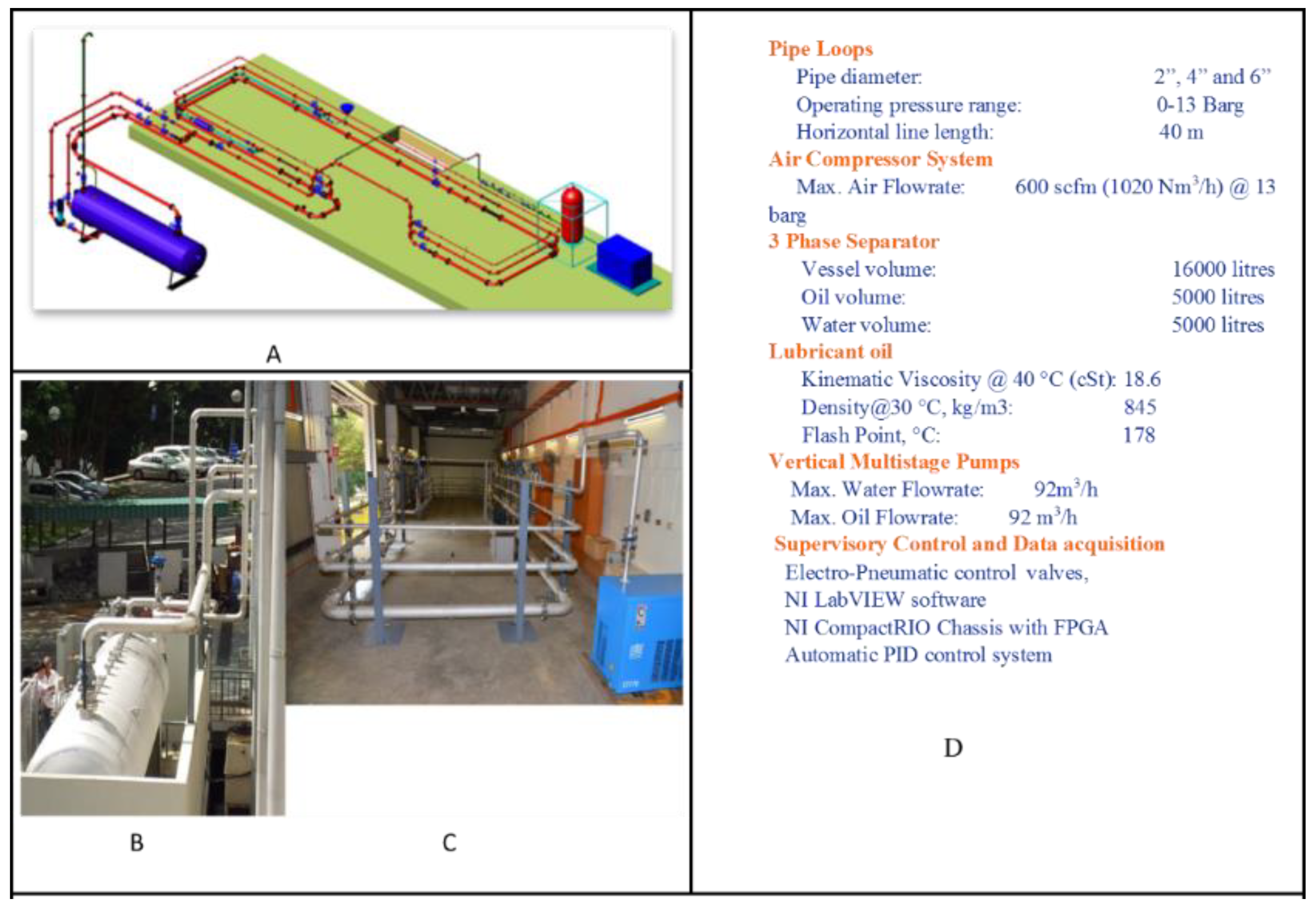
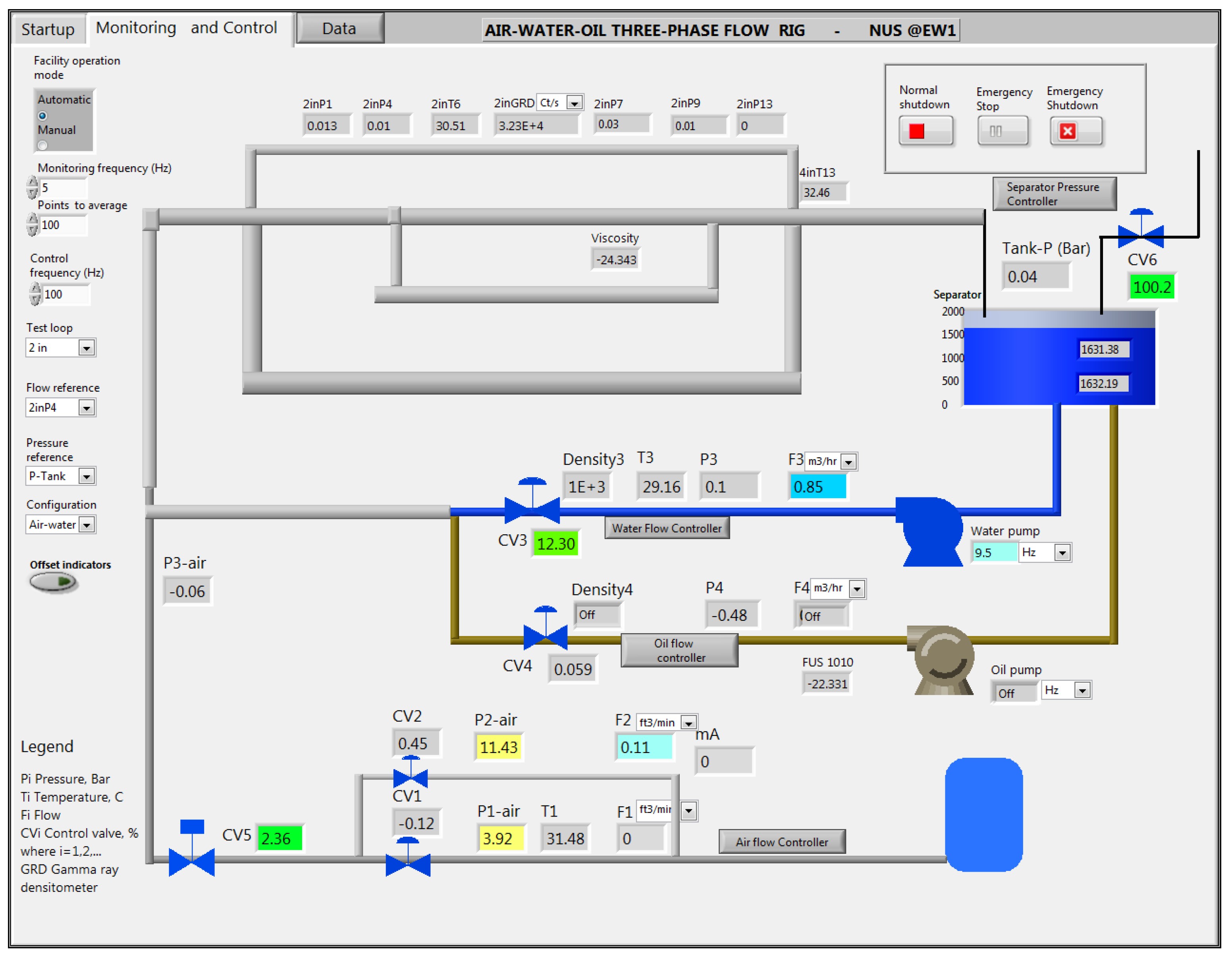
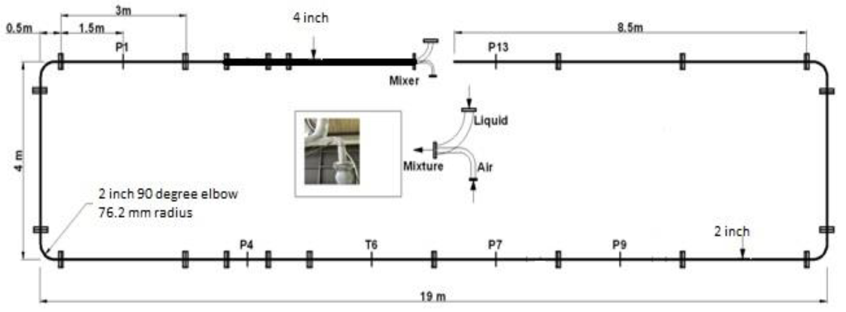
3.1. National University of Singapore (NUS) Experimental Facility, Instrumentation and Data Acquisition

The presented flow loop facility enables three phase flow analysis. Introducing an oil-water-air flow, this facility can be the hub for different studies regarding pipelines, separators, flow meters, pumps, etc. More details about the schematic of the used facility are presented in Figure 3.

To perform multiphase flow studies, indoor measured flow rates of air, water and oil phases are mixed at a pressure rate that can go up to 13 barg. The flow loop has been built using interchanged seamless stainless-steel sections with 3 m length.

To be able to automatically control all variables within the flow loop facility, a compact RIO main chassis is used supplied by National Instruments. As described in [30], the control unit “consists of a real-time processor, a reconfigurable field programmable gate array (FPGA) and the input/output (IO) modules” integrated within a supervisory control and data acquisition (SCADA) software developed within the LabVIEW environment.

To be able to achieve a broader range of flowing conditions, dried air, where humidity has been removed, has been supplied through a parallel circuit containing “two compressors connected in parallel to a receiver tank” [30]. For flow rates measurement two flow meters types are used. For low flow rates (0 to 17 Nm³/h) a differential pressure flow meter is used, although, for high flow rate (0 to 1115 m³/h) a vortex gas flow meter with uncertainty of 1% is employed.

As mentioned above, the three phases flows are controlled using the control software implemented as a Proportional, Integral, Derivative (PID) algorithm within the LabVIEW environment. All the measurements sensors used to control and measure the different properties of the flowing phases (pressure, temperature, and density) along the flow loop are presented in Figure 4.

Within the flow loop, airflow is calculated using the ideal gas equation providing the inlet pressure 2inP1 (Figure 4). Inlet measurements of air pressure and temperature are also collected (T1 and P1-air respectively) as well as in pipe properties (2inP7 and 2inT6). On the other hand, water is circulating from the three-phase separator tank toward the flow loop via a control valve CV3 (Figure 4). Water flow rate and water density are measured using a Coriolis flow meter with “an uncertainty of ±0.3% of the indicated value” [30]. Both phases are then mixed within a mixing section where phases exchange is prevented using check valves.

As detailed in [30], “the test section consisted of a 40 m long loop in a rectangular shape”. To assess the effect of both pressure and temperature, sensors have been placed at different locations along the flow loop as illustrated in Figure 4 and Figure 5.

The NUS flow loop facility is consisted of a rectangular flow loop connected to a three-phase separator tank. This latter tank is used to separate phases and to release the air phase to the atmosphere through valve CV6 as shown in Figure 4, while the liquid phase is redirected toward the flow loop.

Although being a three-phase flow loop facility, all the experimental studies shown in this work are mainly concerning air–water mixtures in horizontal pipelines.

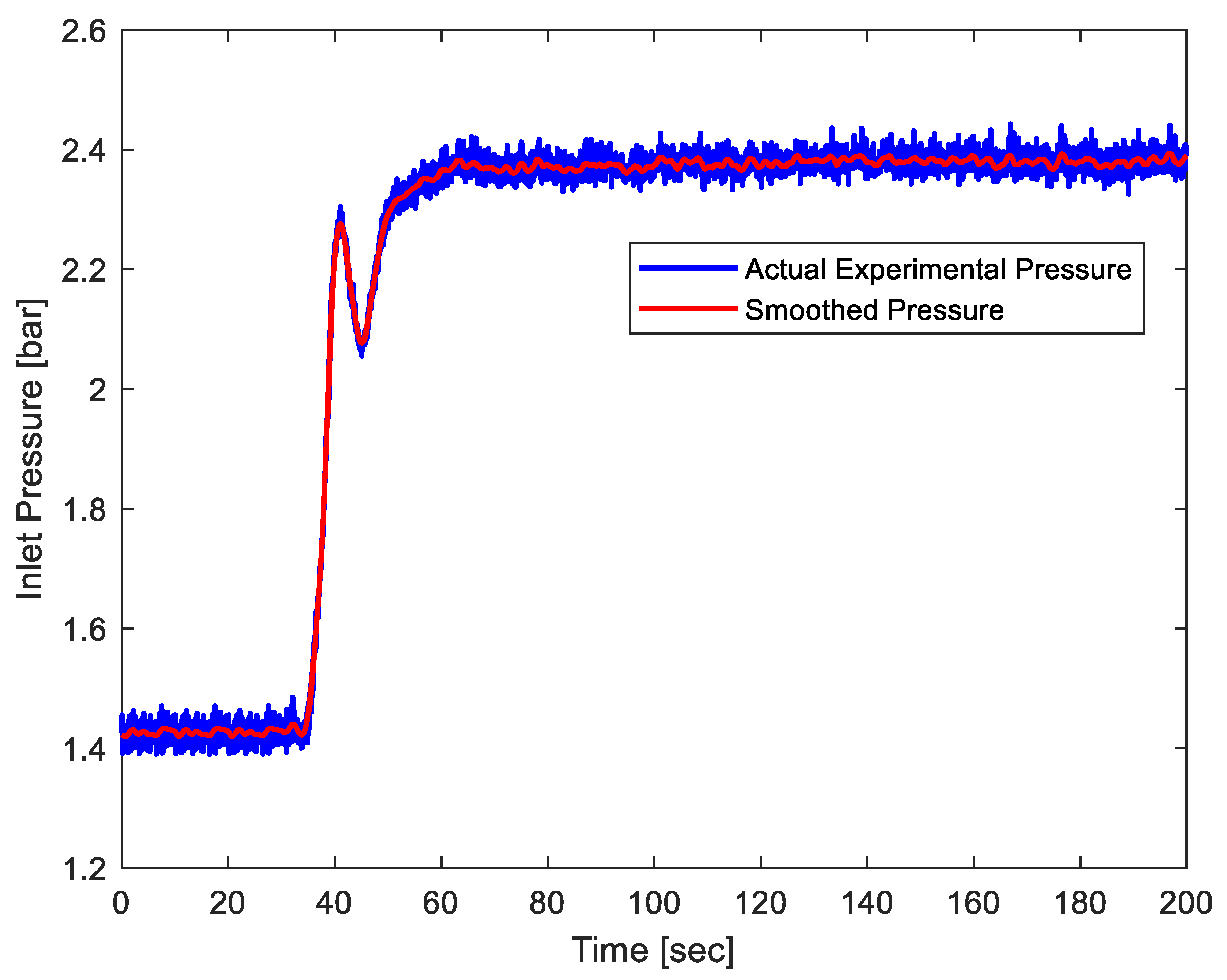
3.2. Dynamic Multiphase Flow Transient Response Evaluation

To minimize sensor noise, a filtering process is implemented. All measured variables were filtered using the weighted average smoothing tricube function:

$$w_i={\left[1-{\left(\frac{abs\left(i\right)}{\frac{npts-1}{2}}\right)}^3\right]}^3$$

(17)

where i and $w_i$ are respectively, the position and the weight associated to the current data point within the sample window. The resulting filtered signal is given by:

$$y_i=\frac{{{\displaystyle \sum }}_{k=-\frac{npts-1}{2}}^{\frac{npts-1}{2}}{w}_{i+k}{y}_{i+k}}{{{\displaystyle \sum }}_{k=-\frac{npts-1}{2}}^{\frac{npts-1}{2}}{w}_{i+k}}$$

(18)

An example of the smoothing procedure for the case of 10% GVF is presented in Figure 6.

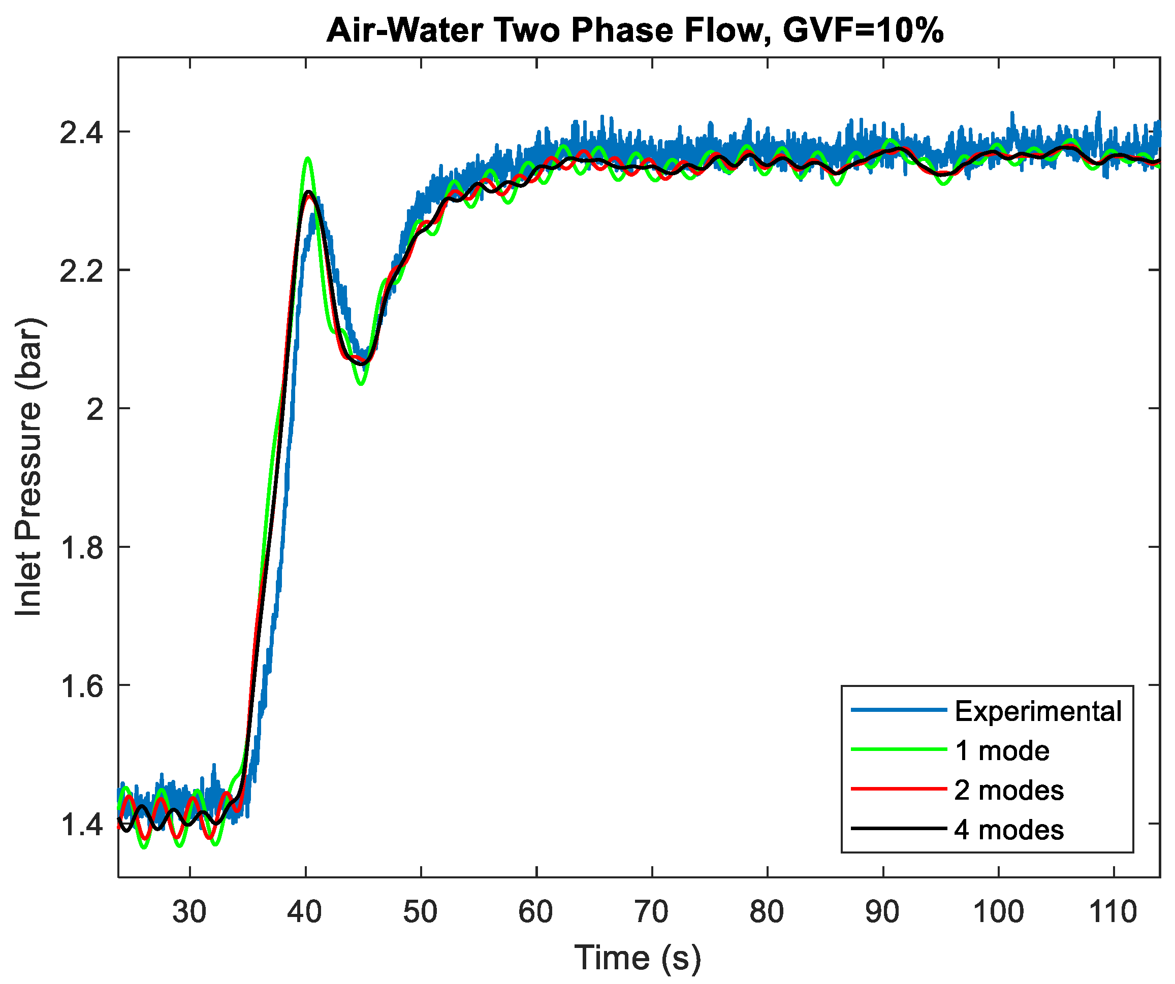
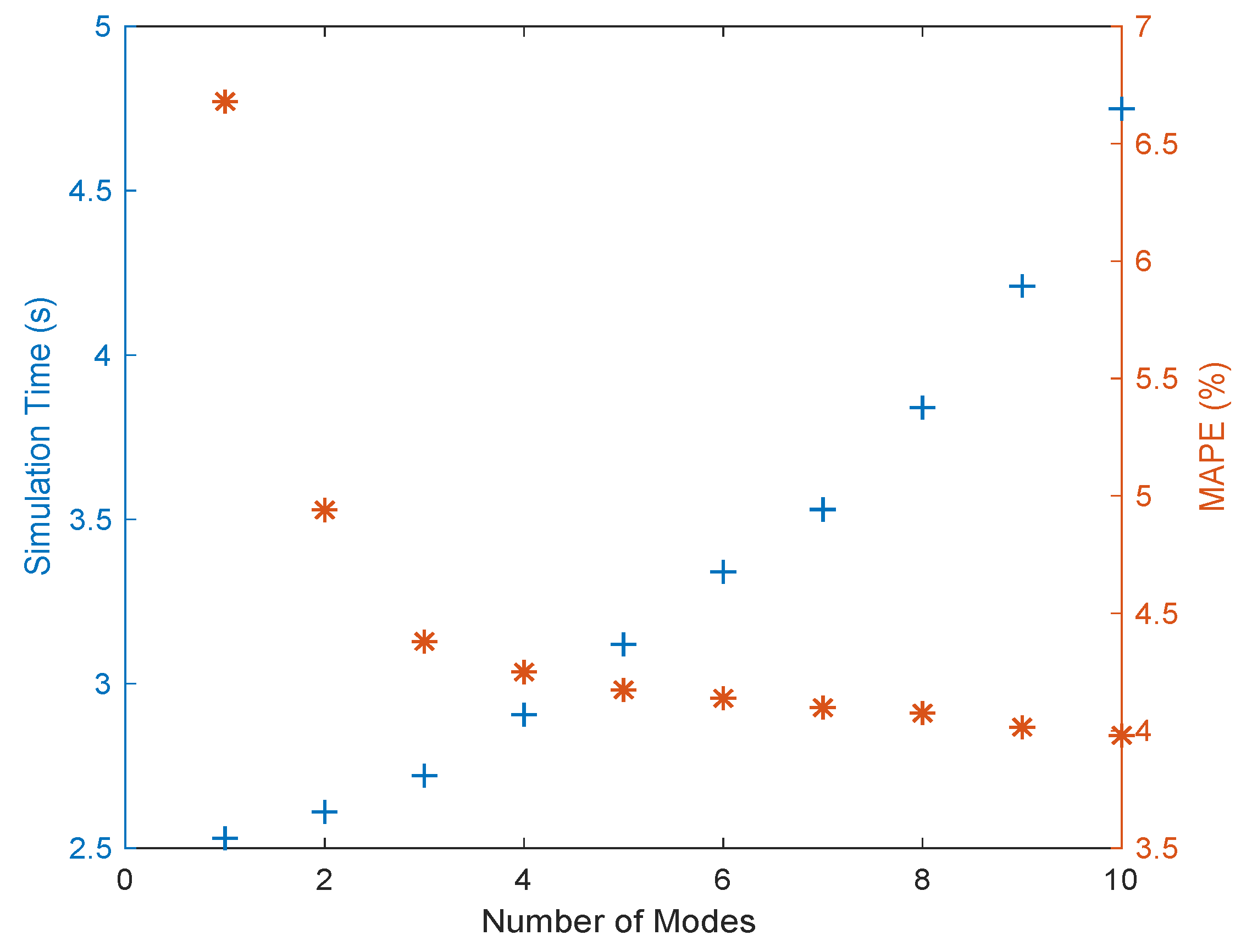
3.2.1. Effect of the Number of Modes on the Low-D Model Accuracy

The authors in [14] investigated the effect of the number of modes based on the estimation given by Equation (10) through sensitivity analysis (Figure 7). The focus of this section is on validating the distributed dissipative low dimensional model predictions with the experimental results for different model orders denoted as n.

Shown in Figure 8 are the computational time and the mean absolute percent error (MAPE) as a function of the number of modes considered in the Low-D model.

The expression used to evaluate the MAPE for a vector X with N values is given as:

$$MAPE=\frac{1}{N}{\displaystyle \sum }_{i=1}^N\left|\frac{X_i^{actual}-X_i^{estimated}}{X_i^{actual}}\right|$$

(19)

where $X_i^{actual}$ is the actual value and $X_i^{estimated}$ is the estimated value.

As the number of modes is increased, the MAPE decreases as a function of the number of modes while the computation time slightly increases. This tendency is inverted when considering a higher number of modes where the computational time increases dramatically without a significant improvement in the model predictions. Hence, selecting the appropriate number of modes is important depending on the desired model application and available computing power. For the remainder of the paper and based on the tradeoff analysis present in Figure 8, four modes will be used to approximate the transfer functions in Equation (10).

3.2.2. Effect of Entrained Air on the Pipeline Dynamic Response

The transient single-phase flow in pipelines has been extensively studied in the literature [27,31]. However, the effect of small amounts of entrained air on the pipeline dynamic response has not been established. Air pockets form inside the pipeline due to bubble entrainment through the action of pump suction or can be released as the pressure of the liquid decreases along the pipeline. Under standard conditions, water can contain up to 2% of entrained air per volume unit [32]. Depending on the application, the effect of entrained air can be either beneficial or detrimental. The presence of air in pipeline systems can result in numerous problems including loss of carrying capacity, disruption of the flow, reduced pump and turbine efficiency or create cavitation problems under low-pressure conditions causing significant damage to the pipeline structure. The speed of waves propagation is also reduced substantially with the presence of air in the pipeline and the damping can be increased allowing a shorter length of the fortified zone required for the high-integrity pressure protection system (HIPPS).

In this section, the NUS multiphase flow loop, the Low-D two-phase flow model [14], and the OLGA multiphase flow simulator [13] are used to investigate the effect of the entrained air on the pipeline dynamic response. Three cases are investigated using the water pump to vary the flow in the loop by stepping the liquid superficial velocity from 0.1 m/s to a pre-specified value while keeping the air compression constant. The summary of the three cases is listed in

Table 2. Liquid superficial velocity variation.

Case Number	Initial Liquid Superficial Velocity (m/s)	Steady-State Liquid Superficial Velocity (m/s)
1	0.1	2
2	0.1	3
3	0.1	4

.

The measured inlet pressure and the those predicted by the Low-D model and the OLGA simulations are given in Figure 9, Figure 10 and Figure 11. Both models show agreement of the steady-state predictions of the inlet pressure due to a step increase in the water flow with the experimental data. However, the Low-D model and the OLGA simulations are characterized by higher frequencies of oscillation associated with higher overshoot.

Note that the amplitude of oscillation decreases from case 1 to cases 2 and 3. This can be explained by a higher turbulent flow energy loss due to the increase of the liquid flow rate. Also, similarly to case 1, both the Low-D model and the OLGA simulations predicted higher frequency oscillation and overshoot. Upon further investigation of cases 1–3, the air velocity sensors are recording low flow rates, suggesting the presence of entrapped air in the system. The presence of entrained air in the pipeline results in a significant increase in the fluid compressibility.

The entrained air is modeled by altering the fluid equivalent bulk modulus. Two models are presented in the literature to account for the effect of the entrained air on the fluid bulk modus. In [31] it was proposed that:

$$\begin{array}{cc}{\beta }_{eq}={\beta }_L\frac{1+r_{\nu }}{1+\left(\frac{P_0}{P}\right)r_{\nu }\frac{{\beta }_L}{kP}}& ;r_{\nu }=\frac{V_{G_0}}{V_{L_0}}\end{array}$$

(20)

where ${\beta }_L$ is the liquid bulk modulus without entrained air, $V_{G0}$ is the entrained air average superficial velocity in the liquid at atmospheric pressure, $V_{L0}$ is the average liquid velocity at atmospheric pressure, $P_0$ is the atmospheric pressure, P is the fluid average pressure, and k is the isentropic exponent (normally, k = 1.4).

In [14], the equivalent bulk modulus of a two-phase flow mixture was characterized as a function of the GVF level. The same equation can be adopted to account for the effect of entrained air (very low GVF) on the equivalent bulk modulus. The pipeline compliance also affects the fluid compressibility [31] as:

$${\beta }^{\prime }=\beta \frac{1}{1+\frac{\beta }{{\beta }_P}\gamma }$$

(21)

where ${\beta }_P$ is the bulk modulus of the pipeline and $\gamma$ is given by:

$$\begin{array}{cc}\gamma =\frac{2\left(\frac{d_0}{d_i}\right)\left(1+\upsilon \right)+3\left(1-2\upsilon \right)}{{\left(\frac{d_0}{d_i}\right)}^2-1}& if \frac{S}{d_0}>0.1 \left(thick walls\right)\\ \gamma =\frac{d_i}{S}& if \frac{S}{d_0}<0.1 \left(thin walls\right)\end{array}$$

(22)

where $d_o$ is the outer pipe diameter, $d_i$ is the inner pipe diameter, $\upsilon$ is the Poisson’s number (0.3 for steel) and S is the pipe wall thickness. Shown in Figure 12 is the water equivalent bulk modulus as a function of the GVF level (up to 2%) using Model 1 evaluated based on Equation (15) and Model 2 (equivalent bulk modulus as present in Equation (1)).

The agreement between the two models in estimating the effect of entrained air on the water bulk modulus is noticed. Both models predict a decrease in the bulk modulus as the first air bubbles are introduced which results in an important increase of the fluid compressibility. The entrained air will also affect the fluid equivalent density as shown in [14]. Shown in Figure 13 is the equivalent density as a function of the GVF level.

The experimental average air and water superficial velocities measured in the flow loop are used to calculate the GVF. The updated equivalent fluid parameters are used as model inputs for the Low-D model for cases 1–3 (

Table 3. Equivalent fluid properties.

Case Number	GVF	Equivalent Bulk Modulus (Pa)	Equivalent Density (kg/m3)
1	0.015	7.12 $\times$ 106	983.55
2	0.016	6.85 $\times$ 106	982.94
3	0.014	7.57 $\times$ 106	984.48

).

In the OLGA simulator, an air feed corresponding to the average air velocity is introduced at the pipeline inlet to account for the entrained air. Shown in Figure 14, Figure 15 and Figure 16 are comparisons between the experimental data and model estimations assuming the presence of entrained air. The introduction of entrained air in the system results in lower natural frequencies and higher damping ratios. This translates to time domain predictions better matching of the oscillation frequency and the overshoot when compared to the experimental dataset.

3.2.3. Effect of Gas Volume Fraction (GVF) on the Pipeline Dynamic Response

The water pump and the air compressors control the superficial velocities achieving GVF levels between 10% and 90%. The measured liquid and air inlet superficial velocities at actual conditions and the outlet pressure are used as inputs for the Low-D model. On the other hand, OLGA simulations require the inputs to be present at standard conditions.

The measured and predicted inlet pressures are provided in Figure 17 for the cases of a GVF range from 10% to 90%. Comparing the 10% GVF case (Figure 17) to the low GVF dataset (GVF close to 0%) (Figure 14, Figure 15 and Figure 16), the inlet transient pressure response is characterized by a smaller transient overshoot caused by higher viscous damping and a decrease in the fluid speed of sound. This feature was captured by the Low-D model and the OLGA simulation. Both OLGA and Low-D model predictions demonstrated agreement with the experimental dataset within a MAPE of 5%. There are noticeable differences in terms of the overshoot transients and the settling time. These differences are attributed to the calculated damping ratio as supported in [14].

To evaluate and compare the overall prediction accuracy of the models, the MAPE with respect to the experimental dataset is provided for GVF levels varying from 10% to 90% (

Table 4. Low-D model and OLGA MAPE comparison.

GVF (%)	MAPE (%)
	Low-D Model	OLGA
10	1.96	2.82
20	3.43	4.25
30	2.91	3.41
40	2.60	3.01
50	3.32	3.82
60	2.12	1.60
70	1.87	1.91
80	1.72	1.79
90	1.63	1.65

). Note that only the pressure transients are considered for accuracy assessment.

4. Discussion

As a higher GVF level is imposed inside the pipeline, the time-averaged pressure drop varies due to the transition between different two-phase flow patterns, the interaction between phases and the friction losses effect. This phenomenon was equally captured by the Low-D and the OLGA models. In the other hand, increasing the GVF results also in an overdamped system for the presented dataset. It has been noticed that the Low-D model gives for most of the experimental validation cases a better estimation of the system’s overshoot when compared to the OLGA simulation. The accuracy of the OLGA simulator improves considerably for the higher-pressure dataset while the Low-D model is characterized by a relatively constant performance. This may be explained by the fact that the closure relationships used in the OLGA model are mostly calibrated using oil and gas high-pressure field data.

Certain assumptions were applied in the presented study. The data presented and discussed in this paper are characterized by low-pressure levels (less than 6 bar) due to the equipment limitations and safety consideration of the NUS multiphase flow loop (maximum pressure rated at 13 barg) whereas the pressure can exceed 500 bars for the case of high-pressure oil and gas production. Similarly, all the tests were performed at temperatures near standard conditions while multiphase flow production fluids can undergo considerable temperature variations especially in the subsea environment. The results were also limited to air-water mixtures. To capture the effect of the pressure, temperature and fluids properties variations on the pipeline dynamic response, the fluid properties are updated for each pressure and temperature condition using a pressure/volume/temperature (PVT) file. The use of physics-based relationships in both the Low-D and OLGA models will also ensure a reduced sensitivity to the operating conditions when compared to purely empirical models since these relationships are not correlated to a specific dataset and analysis can be achieved when investigating different operating ranges. Hence, the conclusions drawn from the comparison between the experimental data and the mathematical models should remain valid at different pressure and temperature conditions or fluids. To validate this assumption, the discussed models should be compared not only to experimental test results but also to field data.

In Figure 17, for the case of 20% GVF, significant slugging is observed in the test section, indicated by the sudden increase of the water flow rate and inlet pressure. This phenomenon is created by the accumulation of water at the bend upstream of the test section before being suddenly pushed by the air pressure. Hydrodynamic slugging is caused by the gas phase flowing at high velocities rate over a slow-moving liquid phase. This results in waves that form on the liquid surface that grow to bridge the entire cross-section of the pipe. Compared to terrain slugging, hydrodynamic slugging is characterized by higher frequency and lower amplitude pressure oscillations. While the terrain slugging is present in the simulated pressure by both models, the hydrodynamic behavior of slug flow is not captured as the Low-D and OLGA models only capture the area-averaged pressure seen by the pipeline. The OLGA slug-tracking module, an additional extension for the OLGA multiphase flow model, can be enabled to track the hydrodynamic slugging behavior.

As shown in Figure 18, a slug flow unit can be defined as a succession of a slug film (stratified or annular flow) and a slug body (dispersed bubble flow).

Like OLGA, a hydrodynamic slug-tracking module can be incorporated to the Low-D model as a future study, especially when extending the present work to cover inclined multiphase flows as well. This module will consider the slug flow structure and its effect on the pipeline’s dynamic response. First, the length of the slug film $L_f$, length of the slug buddy $L_s$, the liquid holdup distribution and the slug unit frequency are estimated. This will enable the derivation of a relationship between the slug flow structure parameters and the pipelines’ and fluids’ physical properties. The resulting slug flow structure estimations are then used as scheduling parameters to switch between a stratified flow model (slug film) and a dispersed-bubble flow model (slug body). This procedure enables the estimation of the pressure fluctuation due to the succession of slug units. The additional slug transient module can be easily disabled if only the average pressure is of interest.

To validate the proposed slug-tracking model, additional transient data will be collected at the NUS flow loop to evaluate the model accuracy in predicting the slug flow structure parameters and the pipeline dynamic response for two-phase slug flows and/or inclined pipeline configuration.

5. Conclusions

In this paper, the transient behavior of air–water two-phase flow mixtures in horizontal pipelines was studied through experimental data and mathematical models. The experimental data were collected from the National University of Singapore multiphase flow loop, a facility that offers a modular structure enabling the study the different GVF levels and flow regimes encountered in oil and gas production.

The comparison between the experimental data with low pressure and the Low-D model predictions permitted the quantification of the effect of the number of modes on the Low-D model accuracy and the simulation time. As expected, increasing the model order (number of modes) results in an improved accuracy but requires a longer computational time. A tradeoff between accuracy and simulation time is, therefore, suggested by the modeling environment depending on the required accuracy and available computational power. The analysis of the single-phase flow experimental dataset established the existence of entrained or entrapped air in the system due to the action of the water pump. It has been shown that the presence of entrained air in the pipeline results in a significantly lower speed of sound of the fluid leading to a considerable increase in the pipeline damping and a decrease in the natural frequency.

The Low-D model pressure predictions and the OLGA simulations were compared to the measured transient pressure for different GVF levels. Both models showed a good agreement with the experimental data with a mean absolute percent error lower than 5%. While the Low-D model is characterized with a relatively constant performance for different pressure conditions, the OLGA model accuracy improved for higher-pressure conditions. Considering this level of accuracy and taking into account the difference between the OLGA multiphase flow model and the Low-D model in term of computational requirements, the proposed Low-D model can be deployed to achieve real-time tasks varying from production monitoring, prediction of pressure and flow rate along pipelines, instantaneous flow pattern tracking as well as coupling with flow assurance models for pipeline integrity management analysis.

As a future step, field data will be collected, aiming at evaluating the effect of the fluid properties, pressure, and temperature variations on the model’s accuracy. A slug-tracking module is also suggested for the Low-D model to simulate the hydrodynamic slugging conditions.

References

1. Pedersen, S.; Durdevic, P.; Yang, Z. Review of slug detection, modeling and control techniques for offshore oil & gas production processes. IFAC Pap. 2015, 48, 89–96. [Google Scholar]
2. Maria, S.; Iyalla, I.; Okulaja, O. Investigating Flow Regimes in High Temperature High Pressure HPHT Gas Subsea Tieback. In Proceedings of the SPE Nigeria Annual International Conference and Exhibition, Online, 11–13 August 2020. [Google Scholar]
3. Beggs, D.H.; Brill, J.P. A study of two-phase flow in inclined pipes. J. Pet. Technol. 1973, 25, 607–617. [Google Scholar] [CrossRef]
4. Hagedorn, A.R.; Brown, K.E. Experimental study of pressure gradients occurring during continuous two-phase flow in small-diameter vertical conduits. J. Pet. Technol. 1965, 17, 475–484. [Google Scholar] [CrossRef]
5. Taitel, Y.; Dukler, A.E. A model for predicting flow regime transitions in horizontal and near horizontal gas-liquid flow. Aiche J. 1976, 22, 47–55. [Google Scholar] [CrossRef]
6. Barnea, D. A unified model for predicting flow-pattern transitions for the whole range of pipe inclinations. Int. J. Multiph. Flow 1987, 13, 1–12. [Google Scholar] [CrossRef]
7. Xiao, J.; Shonham, O.; Brill, J. A comprehensive mechanistic model for two-phase flow in pipelines. In Proceedings of the SPE Annual Technical Conference and Exhibition, New Orleans, Louisiana, 23–26 September 1990. [Google Scholar]
8. Ansari, A.; Sylvester, N.; Shoham, O.; Brill, J. A comprehensive mechanistic model for upward two-phase flow in wellbores. In Proceedings of the SPE Annual Technical Conference and Exhibition, New Orleans, Louisiana, 23–26 September 1990. [Google Scholar]
9. Petalas, N.; Aziz, K. A mechanistic model for multiphase flow in pipes. J. Can. Pet. Technol. 2000, 39. [Google Scholar] [CrossRef]
10. Moore, K.; Rettig, W. RELAP4: A Computer Program for Transient Thermal-Hydraulic Analysis; Aerojet Nuclear Co.: Idaho Falls, ID, USA, 1973.
11. Fisher, A.; Reid, D.; Tan, M.Z.; Galloway, G. Extending the Boundries of Casing Drilling. In Proceedings of the IADC/SPE Asia Pacific Drilling Technology Conference and Exhibition, Kuala Lumpur, Malaysia, 13–15 September 2004. [Google Scholar]
12. Bendiksen, K.H.; Maines, D.; Moe, R.; Nuland, S. The dynamic two-fluid model OLGA: Theory and application. Spe Prod. Eng. 1991, 6, 171–180. [Google Scholar] [CrossRef]
13. Danielson, T.J.; Bansal, K.M.; Hansen, R.; Leporcher, E. LEDA: The next multiphase flow performance simulator. In Proceedings of the 12th International Conference on Multiphase Production Technology, Barcelona, Spain, 25–27 May 2005. [Google Scholar]
14. Meziou, A.; Chaari, M.; Franchek, M.; Borji, R.; Grigoriadis, K.; Tafreshi, R. Low-dimensional modeling of transient two-phase flow in pipelines. J. Dyn. Syst. Meas. Control 2016, 138, 101008. [Google Scholar] [CrossRef]
15. Jayanti, S.; Hewitt, G. Prediction of the slug-to-churn flow transition in vertical two-phase flow. Int. J. Multiph. Flow 1992, 18, 847–860. [Google Scholar] [CrossRef]
16. Falcone, G.; Teodoriu, C.; Reinicke, K.M.; Bello, O.O. Multiphase-flow modeling based on experimental testing: An overview of research facilities worldwide and the need for future developments. Spe Proj. Facil. Constr. 2008, 3, 1–10. [Google Scholar] [CrossRef]
17. King, M.; Hale, C.; Lawrence, C.; Hewitt, G. Characteristics of flowrate transients in slug flow. Int. J. Multiph. Flow 1998, 24, 825–854. [Google Scholar] [CrossRef]
18. Sutton, R.P.; Christiansen, R.L.; Skinner, T.K.; Wilson, B.L. Investigation of Gas Carryover With a Downward Liquid Flow. In Proceedings of the SPE Annual Technical Conference and Exhibition, San Antonio, TX, USA, 24–27 September 2006. [Google Scholar]
19. NTNU. NTNU Multiphase Flow Loop. Available online: https://www.ntnu.edu/ept/laboratories/multiphase (accessed on 20 May 2021).
20. Pedersen, S. Plant-Wide Anti-Slug Control for Offshore Oil and Gas Processes. Ph.D. Thesis, Aalborg University, Aalborg East, Denmark, 2016. [Google Scholar]
21. NUS Multiphase Flow Loop. Available online: https://www.researchgate.net/lab/Wai-Lam-Loh-Lab-Multiphase-Flow-Loop-Wai-Lam-Loh (accessed on 20 July 2020).
22. Petalas, N.; Aziz, K. Stanford Multiphase Flow Database—User’s Manual, Version 0.2; Petroleum Engineering Department, Stanford University: Stanford, CA, USA, 1995. [Google Scholar]
23. Brown, F.T. The Transient Response of Fluid Lines. Asme. J. Basic Eng. 1962, 84, 547–553. [Google Scholar] [CrossRef]
24. Franke, M.E.; Malanowski, A.J.; Martin, P. Effects of temperature, end-conditions, flow, and branching on the frequency response of pneumatic lines. ASME. J. Dyn. Sys. Meas. Control. 1972, 94, 15–20. [Google Scholar] [CrossRef]
25. Johnston, D.N. Numerical modelling of unsteady turbulent flow in tubes, including the effects of roughness and large changes in Reynolds number. Proc. Inst. Mech. Eng. Part C J. Mech. Eng. Sci. 2011, 225, 1874–1885. [Google Scholar] [CrossRef] [Green Version]
26. Oldenburger, R.; Goodson, R. Simplification of hydraulic line dynamics by use of infinite products. ASME. J. Basic Eng. 1964, 86, 1–8. [Google Scholar] [CrossRef]
27. Hsue, C.Y.; Hullender, D.A. Modal approximations for the fluid dynamics of hydraulic and pneumatic transmission lines. In Proceedings of the Fluid Transmission Line Dynamics 1983, Proceedings of the Winter Annual Meeting, Boston, MA, USA, 13–18 November 1983; American Society of Mechanical Engineers: New York, NY, USA, 1983; pp. 51–77. [Google Scholar]
28. Bendiksen, K.; Brandt, I.; Fuchs, P.; Linga, H.; Malnes, D.; Moe, R. Two-phase flow research at SINTEF and IFE: Some experimental results and a demonstration of the dynamic two-phase flow simulator OLGA. In Proceedings of the Offshore Northern Seas Conference, Stavanger, Norway, 26 August 1986. [Google Scholar]
29. Bendiksen, K.; Brandt, I.; Jacobsen, K.; Pauchon, C. Dynamic simulation of multiphase transportation systems. In Proceedings of the Multiphase Technology and Consequences for Field Development Forum, Stavanger, Norway, 26–27 October 1987. [Google Scholar]
30. Loh, W.L.; Hernandez-Perez, V.; Tam, N.D.; Wan, T.T.; Yuqiao, Z.; Premanadhan, V.K. Experimental study of the effect of pressure and gas density on the transition from stratified to slug flow in a horizontal pipe. Int. J. Multiph. Flow 2016, 85, 196–208. [Google Scholar]
31. Wylie, E.; Streeter, V.L. Fluid Transients; McGraw-Hill Co.: New York, NY, USA, 1978. [Google Scholar]
32. Fox, J.A. Hydraulic Analysis of Unsteady Flow in Pipe; Macmillan International Higher Education: London, UK, 1977. [Google Scholar]
Figure 1. Multiphase flow reduced-order model structure.
Fluids 06 00220 g001
Figure 2. Stanford Multiphase Flow Database—variables distributions.
Fluids 06 00220 g002
Figure 3. Schematic views and pictures of the experimental setup: (A) full 3D view, (B) separator tank, (C) pipe flow loops, (D) specifications [30].
Fluids 06 00220 g003
Figure 4. Experimental setup control panel [30].
Fluids 06 00220 g004
Figure 5. Top view schematic of the physical configuration of the 2-inch test loop, mixing section, and instrumentation [30].
Fluids 06 00220 g005
Figure 6. Smoothing procedure results, 10% gas volume fraction (GVF) case.
Fluids 06 00220 g006
Figure 7. National University of Singapore (NUS) experimental results vs. Low-D model predictions as function of the truncation order n, 10% GVF case.
Fluids 06 00220 g007
Figure 8. Simulation time vs. mean absolute percent error (MAPE).
Fluids 06 00220 g008
Figure 9. Experimental vs. simulations (Inlet Pressure, liquid/case 1).
Fluids 06 00220 g009
Figure 10. Experimental vs. simulations (Inlet Pressure, liquid/case 2).
Fluids 06 00220 g010
Figure 11. Experimental vs. simulations (Inlet Pressure, liquid/case 3).
Fluids 06 00220 g011
Figure 12. Equivalent fluid bulk modulus.
Fluids 06 00220 g012
Figure 13. Equivalent fluid density.
Fluids 06 00220 g013
Figure 14. Experimental vs. simulations (Inlet Pressure, liquid with entrained air/case 1).
Fluids 06 00220 g014
Figure 15. Experimental vs. simulations (Inlet Pressure, liquid with entrained air/case 2).
Fluids 06 00220 g015
Figure 16. Experimental vs. simulations (Inlet Pressure, liquid with entrained air/case 3).
Fluids 06 00220 g016
Figure 17. Pipeline dynamic response evaluation: slug flow (GVF = 10% to 60%), froth flow (GVF = 70% to 90%).
Fluids 06 00220 g017
Figure 18. Slug flow unit schematic [31].
Fluids 06 00220 g018