Article

Discrete Vortex Prediction of Flows around a Cylinder Near a Wall Using Overlapping Grid System

1
Ocean Engineering Department, Institut Teknologi Sepuluh Nopember, Surabaya 60111, Indonesia
2
Marine Engineering Department, Institut Teknologi Sepuluh Nopember, Surabaya 60111, Indonesia
3
Indonesian Hydrodynamic Laboratory, BPPT, Surabaya 60111, Indonesia
*
Author to whom correspondence should be addressed.
Fluids 2021, 6(6), 211; https://doi.org/10.3390/fluids6060211
Submission received: 28 March 2021 / Revised: 22 April 2021 / Accepted: 23 April 2021 / Published: 8 June 2021

Abstract

:
Modelling of unidirectional and oscillatory flows around a cylinder near a wall using an overlapping grid system is carried out. The circular grid system of the cylinder was overlapped with the rectangular grid system of the wall. The use of such an overlapping grid system is intended to reduce the CPU time compared to the cloud scheme in which vortex-to-vortex interaction is used, i.e., especially in calculating the shedding vortex velocity, since calculating the vortices velocity takes the longest CPU time. This method is not only time efficient, but also gives a better distribution of surface vorticity as the scattered vortices around the body are now concentrated on a grid point. Therefore, grid-to-grid interaction is used instead of vortex-to-vortex interaction. Velocity calculation was also carried out using this overlapping grid in which the new incremental shift position was summed up to obtain the total new vortices position. The engineering applications of this topic are to simulate the loading of submarine pipeline placed close to the seabed or to simulate the flow as a result of the scouring process below the cylinder since there is space for the fluid to flow beneath it. The in-line and transverse force coefficients are found by integrating the pressure around the cylinder surface. The flow patterns are then obtained and presented. The comparison of the results with experimental evidence is presented and the range of good results is discussed.

1. Introduction

Various studies involving cylinders in close proximity to an impermeable surface have been conducted using computers and laboratories in the last five decades. Using the discrete vortex method, it is indicated that the best agreements are at G/D = 0.2 and G/D = 0.5, where G is the gap and D is the diameter of the cylinder [1]. The results show that the interaction between the lee-side recirculating flow and the gap flow, which inhibits large-scale vortex roll-up, is developed behind the cylinder. Furthermore, the results at G/D = 1.0 indicate cancellation of opposite signed vorticity in the near-wall region.
A boundary shear flow in proximity of a circular cylinder is numerically investigated using a finite element method [2]. It has a strong effect on the flow behind the cylinder and also the force acting on the cylinder. The variation of the Reynolds number and gap ratio also have a significant role. In this investigation, with a fixed Reynolds number, the drag force increases as the gap spacing decreases. The lift force decreases at a fixed gap ratio, and the drag force varies with a change in Reynolds number. The lift force decreases as the Reynolds number increases.
The flows around two cylinders in close proximity under the influence of the initial conditions using a finite element-based program at low Reynolds numbers, have also been investigated [3].
Another research at low to moderate Reynolds numbers using a numerical model based on 3D RANS simulation was carried out [4]. The drag coefficient increases as the cylinder approaches the wall until G/D = 1. However, as soon as the cylinder became closer than G/D = 1, the flow was submerged into the wall’s boundary layer, and the mean drag coefficient decreased as the base pressure also decreased.
An investigation employing a high Reynolds number and moderate to large gap ratio has also been carried out [5]. This investigation utilized large eddy simulation (LES) using Re = 13,100. At a moderate gap ratio, it yields a long and nearly stationary separation bubble. While the development of gap ratio yields an asymmetric wake with a long shear layer, the bigger gap ratio allows a symmetric flow near the wake to occur.
The vibration of a cylinder near a wall using a partition iterative scheme was studied based on the Petrov–Galerkin formulation [6]. This was carried out to simulate flow past a freely vibrating circular cylinder placed in proximity to a stationary plane wall. The wall proximity effect on vortex-induced vibration (VIV) of an elastically mounted circular cylinder with 2D were systematically studied in two-dimension laminar flow at low Reynolds number. Hydrodynamic forces, vibration characteristics phase relation and response frequencies were also studied.
Another variation is by using an oscillatory flow [7]. This condition was investigated by exposing a cylinder, placed near a wall, to an oscillatory flow and then the span-wise correlation was calculated based on the cylinder surface. This investigation indicated that the effect of wall proximity is insignificant, especially when the fluctuations in surface pressure are taken into consideration.
In this study, further developing the image method by [8], a simple overlapping polar grid system was used for the cylinder to give a good definition of the flow close to the cylinder surface. The grid node on the cylinder surface located at the center of the surface element provides the control points at which the Martensen equation is solved to give zero tangential velocity and satisfy the Dirichlet boundary condition [9].
A potential flow scheme has been used to model this kind of configuration for a low range of Reynolds numbers [10]. In this model, there is no separation model, and the flow resembles a stream-line flow. The force coefficients can then be calculated through the use of the Blasius equation by directly substituting and integrating the complex potential around the cylinder.

2. Basic Formulation

In this study, with only a wall below and near the cylinder, the complex potential equation can then be approximated as follows:
ω ( z ) = u e i + i 2 π e = 1 N e γ e d S e ln ( z z e ) + 1 2 π w = 1 N w 1 σ w 1 d S ω 1 ln ( z z ω 1 ) +   i 2 π υ = 1 N ν Γ ν ln ( z z ν )
The strength of a vortex γ n around the cylinder and a source σ w 1 at element w of the wall g in this equation can be calculated by satisfying the Dirichlet boundary condition of zero tangential velocity on the cylinder surface and the Neumann boundary condition of zero normal velocity along the wall. M w   shows the number of walls, in this case equal to 1 since the wall is only placed below the cylinder, in which N w 1   shows the number of elements of the bottom wall.
As there are two different boundary conditions imposed on the circumference of the cylinders and on the walls, the Martensen equation can be written into two expressions to take into account the influence of the wall:
1 2 γ m + c k m n γ n d S n + c k m w σ w d S w + u . d S m + v N v l m v Γ v = 0
1 2 σ υ + c k v n γ n d S n + c k v w σ w d S w + u . d S v n + v N v l υ v Γ v = 0  
in which k υ n , k υ w , and k m w are the kernels of the integral. σ w is the strength of the wall source at point w, d S m is the tangential direction vector of the cylinder element m, while d S υ n is the normal direction vector of the wall element v.
The velocity of a vortex can then be calculated through the use of the polar and the rectangular grid nodes. The contribution from the wall sources is implemented using the rectangular grid nodes. This implies that a bilinear interpolation and re-interpolation in polar and rectangular coordinates are needed to distribute and redistribute the vortex strength and velocity onto two grid nodes. The force coefficients can then be calculated by integrating the pressure distribution from the point of stagnation to the vicinity of the cylinder surface.
Due to the nature of the kernel functions above, which are asymptotically equal to zero as the distance approaches infinity, the integration reduces to the integrals around the cylinder surface and the wall. It can be seen from Equations (2) and (3) that the Martensen equation cannot be solved independently since each equation contains two unknowns, γ n   and σ w . Therefore, the Dirichlet boundary condition of zero tangential velocity on the circumference of the cylinders implied in Equation (2) and the Neumann boundary condition of zero normal velocity along the walls implied in Equation (3) must be solved simultaneously.

3. Methodology

3.1. Surface Velocity Calculation

As the source strength far away from the cylinders are relatively small, their contribution is neglected beyond a cut-off at a certain finite distance from the cylinders, which produces a finite number of wall elements Nw, as follows:
n = 1 N e k m n γ n d S n + w = 1 N w k m w 1 σ w 1 d S w     1 + ( u e i ( β m ) ) + v = 1 N v l m v Γ v = 0
to satisfy the Dirichlet boundary condition at element m of the cylinder circumference and
n = 1 N e k v n 1 γ n d S n + w = 1 N w k m w 1 σ w 1 d S w     1 + ( u e i ( β v g ) ) + v = 1 N v l v v g Γ v = 0
to satisfy the Neumann boundary condition at element v of the wall g. To find the unknown value of the vortex strength γ n   and the source strength σ w , these equations can now be expressed in the matrix form as follows:
( K m n K m v 1 K v n 1 K v 1 v 2 11 ) ( γ n σ v 1 ) = ( R H S R H S 1 )
where the components inside the matrix are all submatrices with 1, signifying the bottom wall.

3.2. Segmentation of the Domain

It can be seen from Equation (1) that after shedding vortices, the order of Nw operations must be carried out when performing the velocity calculation for a vortex due to the contribution of only a wall source and the number of operations will be this velocity calculation for a vortex added by Nv + 1, the number of vortices in the flow, if mutual vortex interaction is used. The final total number of operations will be this number multiplied by the number of shed vortices Nv.
Using rectangular grid nodes as shown in Figure 1 below, this number could be reduced by replacing the factor Nv + 1 with j , k N j , k + 1 , which is obviously a smaller number. About the same amount of CPU saving can also be found during the source strength calculation in the component of Equation (6) from the contribution of the shed vortices, which also use the rectangular grid elements.
It is shown in Figure 1 that the size of the rectangular grid segment is arranged in order of the length of the wall source element. This means that the rectangular wall elements are uniform throughout the whole fluid domain. The first row of the rectangular grid nodes next to the wall are arranged in such a way as to give the best visualization of the flow pattern.
The polar grid coordinate is extended up to 65 segments. The lower part of the polar grid coordinate below the bottom wall is removed. The active polar grid coordinate is dependent on whether there is vortex or not in the grid; in this case, the grid node is designated as ‘on’. Otherwise, if there is no vortex in the grid, in which case, the grid node is designated as ‘off’. In this calculation process, we cannot exactly calculate the number of grids as the grid can be either on or off. The same reason is also applied to the rectangular grid.
The time step chosen was t ^   = Ut/D = 0.15. The effect of spatial time and time step is optimal when the number of elements of the cylinder is 64. If the number of elements of the cylinder is smaller, it seems that the picture of the flow produced is too coarse. On the other hand, if the number of elements of the cylinder is greater than 64, the amount of vortex shedding is too large. The length of the rectangular grid node segment is made similar to the length of the elements of the cylinder. If the time step is less than 0.15, then the number of vortex shedding is also too large. On the other hand, if the time step is greater than 0.15, then the flow pattern is too coarse.

3.3. Introduction of Vortices into the Flow

The discrete vortices are introduced into the flow so that the position of separation and the trajectory of the separated shear layer are consistent with the experimental results. In fact, these are determined by complex fluid motions in the boundary layer involving a delicate balance between convection and diffusion with the additional important influence of the local surface static pressure gradient.
The presence of the walls in close proximity to the cylinder obviously changes the wake behaviour behind the cylinder. This is partly due to the effective increase in local velocity and partly due to interference from the reflected periodic wake. In this present simple model, only the ’blockage’ effect is considered and all the effects of the boundary layer interaction between the cylinder and the wall are ignored. The effects of Reynolds number are implicit in the choice of various model parameters such as the element lengths and grid dimensions. These have been largely specified on the basis of previous works [8,11], as well as the sensitivity studies.

3.4. Distribution of Circulation on to the Grid

The strength of a vortex is distributed in its own surrounding polar grid nodes and rectangular grid nodes. A vortex shed from the cylinders is distributed in the same manner and stored in a different array. The polar grid nodes are used to evaluate the interaction among vortices shed from the cylinder while the rectangular grid nodes are used to evaluate the influence of wall to the vortices.
It can be seen from Figure 1 that the use of polar grid elements close to the wall could create a situation where an active polar grid node is situated outside the fluid domain between the walls, even though the vortex it represents is still inside. This active node is then treated as usual, bearing in mind that the active nodes only represent a redistribution of vortices in the flow and also that there is no direct interaction between the polar grid nodes and the wall elements.

3.5. Random Walk Method

The random walk method has been widely used to model the viscous diffusion of high Reynolds number flow using the discrete vortex method [12,13]. The basis of this scheme is to give a random displacement to each vortex to produce a scatter equivalent to the diffusion of vorticity in the continuum.
In two dimensions, the solution of the diffusion equation is the vorticity decay of a line vortex as follows:
ω ( r , t ) = Γ 4 π v t e x p ( r 2 4 v t )
Equation (7) is a function of radius r and time t. Hence, the vorticity decays as the distance from its center increases and it also decays as the time increases. In this equation, Γ is assumed to consist of a large number of small vorticity elements, all initially located at the origin, but are free to diffuse outwards independently of one another over a period of time. This equation is regarded as a vorticity density probability distribution curve to be matched by the random displacements to which we will subject the small elements during the numerical diffusion simulation process [14,15].
Due to the r2 factor, it can be seen that the vorticity decay equation is an even function relative to its center. If Equation (7) is integrated in terms of the area of a circle whose center is at the vorticity center, it will result in:
P ( r , t ) = 1 e x p ( r 2 4 v t )
in which P states the probability that a given element will lie somewhere within a circle radius r and this equation also represents the Gaussian normal distribution of zero mean and a standard deviation of 4 v t . It follows from this that given two random numbers P1 and P2, within the interval (0,1), the values
r = 4 v Δ ln 1 1 P 1
and
θ = 2 π P 2
δ z v r ω = r e i θ
will give representative displacements for a group of vortices in radial and angular direction under this distribution of probability. Hence, the influence of the Reynolds number is represented in the form of a diffusion process.

3.6. Calculation of Velocity

The complex velocity at a point z = x + i y   in the flow field is simply the derivative of Equation (1) as follows:
d w ( z ) d z = u i v = u e i a + i 2 π n = 1 N e γ n d S n z z n + 1 2 π h = 1 M w w = 1 N w h σ w h d S w h z z w h + i 2 π v = 1 N v Γ v z z n
in which u and v are the velocity components in x and y directions, respectively. As explained previously, there is no direct vortex-to-vortex interaction in calculating the velocity in the field domain, only a grid-node-to-grid-node interaction. This process is carried out to reduce the great number of vortex-to-vortex interactions. This can be reduced by the grid-node-to-grid-node scheme system which has a much smaller number of interactions. Thus, the grid-node-to-grid-node scheme must have a lesser CPU time since the interaction involved is smaller. As the calculation of vortex velocity is carried out after the introduction of vortices into the flow, this equation has to be modified slightly by eliminating the second term of Equation (12) as the surface vorticity has already been released and absorbed in the shed vortices Nv as follows:
d w ( z ) d z = u i v = u e i a + 1 2 π h = 1 M w w = 1 N w h σ w h d S w h z z w h + i 2 π j , k Γ j , j k z z j , k  
in which z j , k shows the coordinate of the active grid nodes either in relation to the polar or the rectangular grid system. The source contribution in the second term of the equation is carried out through the use of the overlapping rectangular grid system. The velocity of the active rectangular grid nodes due to the source distribution of the walls is then
u ¯ w ( z ) = 1 2 π h = 1 M w w = 1 N w h σ w h d S w h z z w h
where N w h   is the total number of elements at wall h.
The velocity of a vortex v shed from the cylinder due to the wall is then found through the use of the following bilinear interpolation:
u ( z v ) = u v ( z v ) + u p w ( z v ) + u r w ( z v )
where u v ( z v ) is the vortex velocity due to other vortices shed from the cylinder, u p w ( z v ) is the vortex velocity due to the influence of the walls and u r w ( z v ) is the vortex velocity due to the diffusion of the random walk above.

3.7. Time Integration

A first order accurate Euler scheme is used to find the new locations of the vortices, as follows:
z v ( t + Δ t ) = z v ( t ) + δ z v r w + δ t u v ( t ) ( z v )  
where z v ( t ) is the initial position, δ z v r w is the increment due to the random walk scheme above [9] and δ t u v ( t ) ( z v ) is the increment due to the convection scheme.
Since an overlapped grid system is used in the scheme, the new position of each vortex is then referenced to both the polar and rectangular grid systems. In other words, each vortex has two base nodes from which its relative position at every time step is measured and renewed.

3.8. Force and Pressure Calculation

The force calculation can be carried out after the convection and diffusion processes by solving the following equation:
u t = 1 ρ p
and hence,
p = p s S 1 S ρ γ ( S ) t d S
which is derived from the Navier–Stokes equation on the basis that at any point Sn in the cylinder surface, the velocity parallel to the surface is given by u t = γ n . From that equation, a numerical expression for the change in surface pressure over the element n during the discrete time step Δt can then be obtained as:
Δ p n = ρ γ n Δ S n Δ t = ρ Γ n Δ t
The difference of pressure Δ p n   is measured from the stagnation pressure p s = 1 2 ρ u 2 at the stagnation point Ss. Hence, the pressure at element m will be
p n = p s ρ Δ t n = 1 m Γ n
The other force that contributes to drag and lift forces is the one due to the skin friction (viscous drag) on the surface of the cylinder, as follows:
τ n = μ ω n = μ γ n d S n d A n
where µ is the dynamic viscosity.
The form drag, lift and skin friction coefficients can be calculated as follows:
C D = D 1 2 ρ u 2 d = 2 ρ u 2 d n = 1 m ( p ¯ n sin β n Δ S n + τ ¯ n cos β n Δ S n )
C L = L 1 2 ρ u 2 d = 2 ρ u 2 d n = 1 m ( p ¯ n cos β n Δ S n τ ¯ n sin β n Δ S n )
where d is the diameter of the cylinder and β is the tangent angle of the element. The basic procedure is based on the integration of the elemental pressure around a cylinder. The pressure around the cylinder then can be integrated numerically to obtain the value of the force coefficients.

3.9. Method of Enhancement

Theoretically, the source wall distribution should extend from   to   as expressed in the continuous form of the Equations (2) and (3) above. However, lim x σ w ( x ) = 0 or in other words, the blockage effect experienced by the cylinder due to the presence of the wall is small at distant points. The wall is modelled by source extending along the wall until a point when the mutual interaction between the distant wall elements and the cylinder or shed vortices is relatively small.
The influence of the number of sources modelling the wall on the fluid velocity just outside the cylinder surface element closest to the wall are shown in Figure 2. It can be seen that the rate of change of the cylinder surface vorticity strength γ k   to the wall extension γ k x w = 0   is less than 0.01, when the distance of the end wall elements to the cylinder center is greater than 3D. This value is then used to determine the wall length after shedding vortices. The wall end points can be determined by measuring this distance from the extreme position of a vortex.

4. Results and Discussion

4.1. Uni-Directional Flow

Experiments in a wind tunnel were conducted under a Reynolds number of 4.5 × 10⁴ for the flow around a circular cylinder placed at various heights above a plane boundary [16]. It was revealed that regular vortex shedding persisted at the Strouhal number St = Uf/D for all gaps down to G/D = 0.3. For all values of G/D < 0.3, strong regular vortex shedding began to be suppressed, and when the cylinder touched the wall, there was no regular shedding of vortices.
As the cylinder was moved away from the wall, the pressure distribution around the cylinder became more symmetric near the stagnation point and at G/D = 0.4 it was perfectly symmetric. At small gaps, the separation point on the side nearest to the wall moved down stream to the narrowest point of the gap. The flow around a cylinder close to a wall can be considered to be analogous to the flow around two cylinders in a side-by-side arrangement. For G/D > 0.5 the two flows were similar. However, the flow around two cylinders becomes bi-stable for G/D < 0.5, whereas a cylinder near a wall shows no such in-stability.
The flow pattern of a cylinder near a wall at various gaps of 0, 0.2, and 0.4 diameters were reproduced from the experiment results [12]. It is shown in Figure 3, copyright by [12], that suggested this reduction is mainly caused by the interference of the wall with the vortex shedding and the immersion of the cylinder in the lower energy wall-boundary layer flow.
However, their data appears to reveal an upward trend in the recorded values of the Strouhal number of approximately 5% at a gap of 0.75 diameters. It is argued that this effect is caused by a reduction of the scale of the vortex formation region due to the proximity of the wall, and that when the shear layers are brought closer together, their interaction is facilitated, and the shedding period is shortened [17]. Variation of vortex shed-ding frequency as a function of wall distance from the cylinder are plotted in Figure 4, which shows that the shedding frequency gradually increased as the gap decreased. A 10% increase of shedding frequency is expected when the gap is very small.
It is shown that when the gap ratio G/D is greater than 2, the cylinder behaves similar to an isolated cylinder due to the influence of the wall being relatively low. Based on these experimental studies, the model was tested at a high Reynolds number of 100,000 and at several gap ratio values of 2.0, 1.5, 1.0, 0.5, 0.25, 0.1. At the first gap ratio G/D = 2 and at the non-dimensional times of 1 and 5, the flow behind the cylinder is shown in Figure 5.
In this study, the separation point close to the wall is shifted downstream to about 125 degrees, while the one on the top side of the cylinder surface is shifted upstream to about 135 degrees, measured from the positive X-axis. The shear layer emanating from the lower half of the cylinder seems to stretch longer than the upper one, even though no forced asymmetry was implemented. The formation region also seems to be slightly longer than that of an isolated cylinder by about 5 to 7%. This is due to the fact that the close presence of the wall creates an asymmetric velocity field around the circumference of the cylinder in which the velocity of the fluid particles close to the wall are relatively higher than the rest. The asymmetric velocity field around the cylinder also promotes the roll-up of the vortices earlier than that of the isolated cylinder.
As the flow further develops, a regular vortex shedding is clearly established, and this is also reflected in the graph of the force coefficients. The drag coefficient is slightly less than 1.14, which is the value for an isolated cylinder, and the lift coefficient oscillates around a mean value of about 0.15 with the Strouhal number relatively unchanged from 0.2. The steady flow implies that a repulsive force exists in the direction which tend to displace the cylinder away from the wall. The obvious difference between this flow pattern and that of an isolated cylinder is that the vortices close to the wall tend to approach it tangentially, follow it and then leave it tangentially as well, while those on the other side are freely convected, similar to an isolated cylinder. Numerically, this is obviously due to the source distribution along the wall. It tends to reflect the vortices close to it back to the fluid domain.
This is also shown in the calculation in that generally, when the vortices are close enough to the wall, the strength of the sources in that region are positive (sources), while those in the region sparsely populated by vortices show negative values (sinks).
The CPU time taken at each section is shown in Table 1. It is shown that the percentage of time taken to calculate the vortex velocity is the greatest, up to 73.97%. The second biggest CPU time is the calculation of the cylinder surface velocity, as much as 16.03%.
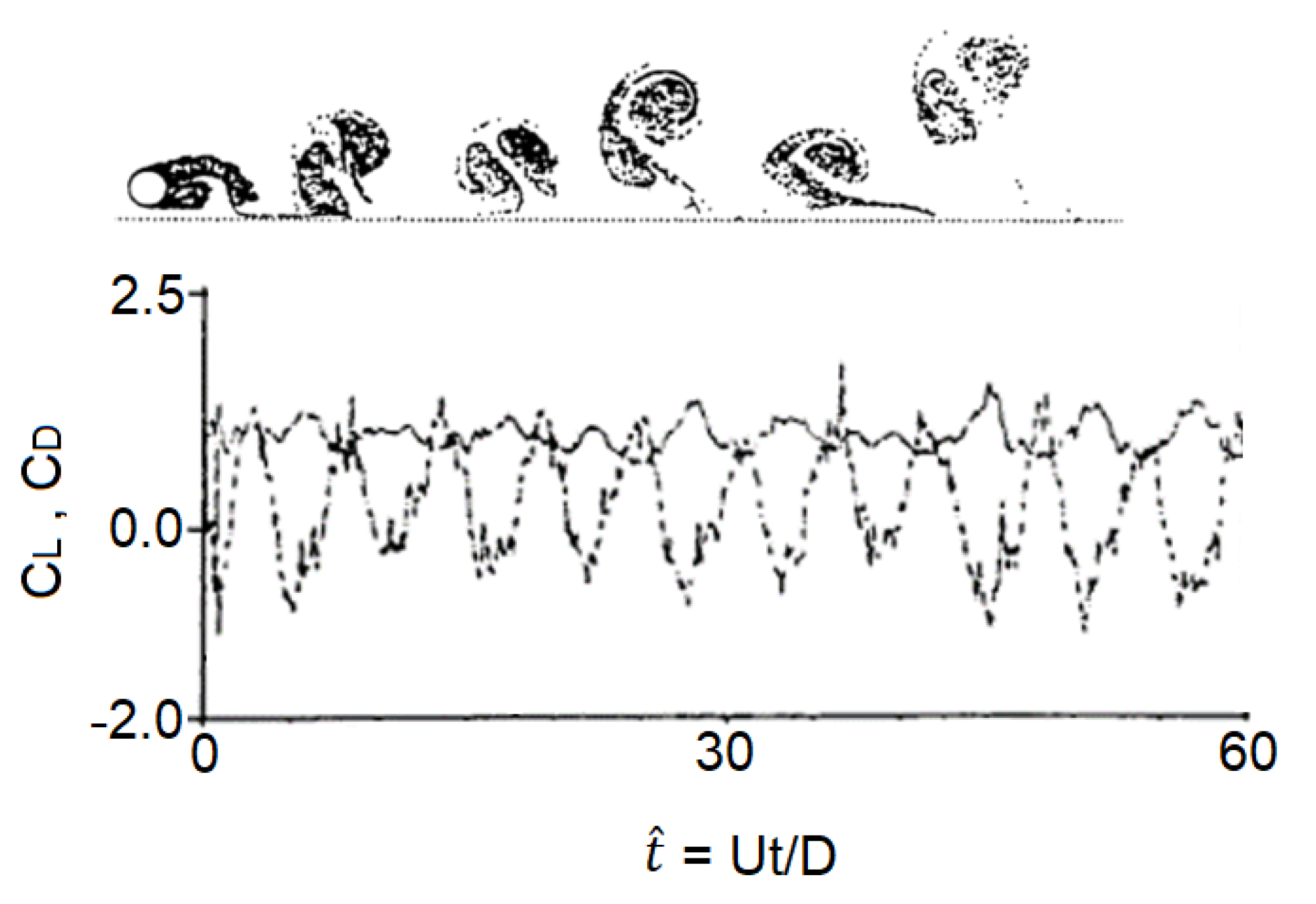
The influence of the wall on the hydrodynamic characteristics of the cylinder increases as the gap ratio is reduced to 1.5, 1, 0.75, 0.5 and 0.25, as shown in Figure 6, Figure 7, Figure 8, Figure 9, Figure 10 and Figure 11. The drag coefficient decreases to 1.13 and the mean value of the lift coefficient is around zero, in which these values are those of the isolated cylinder.
The cylinder can be seen to be increasingly deflected in a tangential direction as the gap between the cylinder and the wall is decreased. It is also shown in these figures that as the velocity in the gap region increases, vortices with high strengths are created, which in turn produces a strong mutual interaction. This results in a higher velocity in the region along the wall behind the cylinder, which then causes the vortex street to be deflected as the vortices close to the wall move further away from those located further into the flow.
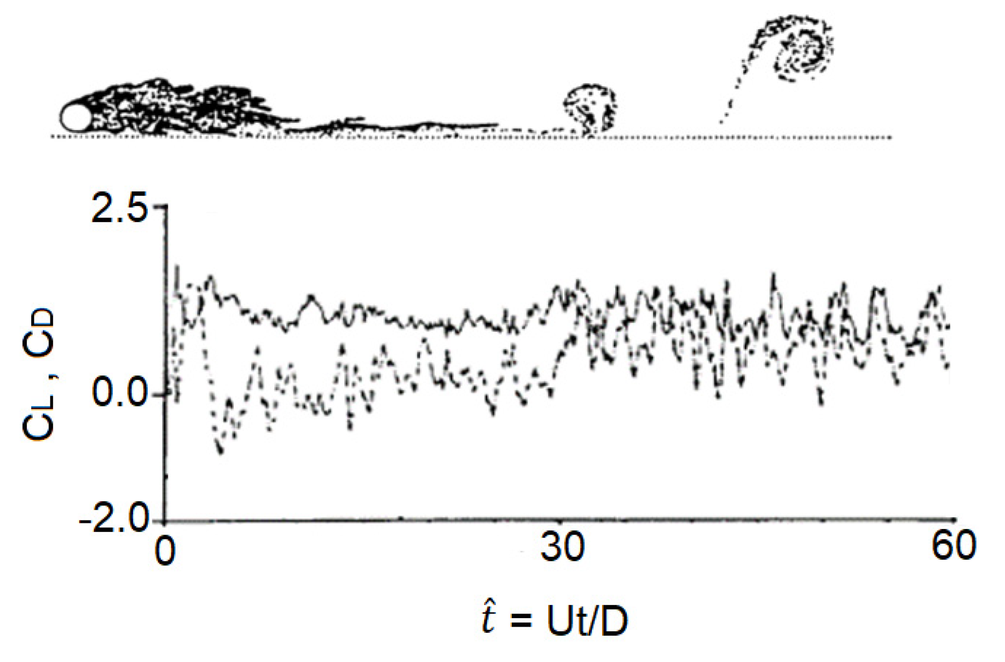
An asymmetric effect further occurs when the gap ratio G/D is reduced to 0.25 and the influence of the wall as described above is further pronounced. The vortex street becomes more skew-symmetric due to the greater influence of the wall, which is reflected in the higher velocity in the gap region, as shown in Figure 11. It can also be seen that the repulsive force, shown as the average lift coefficient, is higher and reaches 0.75 with a Strouhal number equal to 0.17 and the drag coefficient slightly increases to 1.45. Experimental evidence shows that when the gap ratio G/D < 0.15, regular vortex shedding is suppressed due to the complicated behavior of the turbulent boundary layer interaction in the gap region.
Flow visualization, hot film and PIV experiments have been conducted to investigate the flow around a circular cylinder with a close proximity to a wall for Reynolds numbers in the range of 1200 ≤ Re ≤ 4960 [18]. The results revealed that four distinct regions may be identified for describing the flow within the observed flow dynamics. For very small gap ratios, G/D ≤ 0.125, the gap flow is either suppressed or extremely weak, and no regular vortex shedding occurs downstream of the cylinder. This condition is not tested in this present study. The flow field for small gap ratios, 0.254 ≤ G/D ≤ 0.375, is very similar to that for very small gap ratios, except that there is now a pairing between the inner shear-layer shed from the cylinder and the separated wall boundary layer. Intermediate gap ratios—0.54 ≤ G/D ≤ 0.75—are characterized by the onset of vortex shedding from the cylinder. In addition, there is a significant decrease in the size of the upstream separation region. For the final region, characterized by the largest gap ratio considered, G/D ≥ 1.0, there is no separation of the wall boundary layer, either upstream or downstream of the cylinder. In addition, the flow around the cylinder is now essentially the same as the flow around an isolated circular cylinder. The variations of the Strouhal numbers with respect to the gap ratio is very dependent on the Reynolds number. For low Reynolds number flows, Re = 2600, the Strouhal number for G/D ≤ 2.0 is significantly greater than that of an isolated circular cylinder. However, for higher Reynolds numbers (Re = 4000) St seems to be insensitive to G/D. In contrast to other studies, there does not seem to be a minimum value of G/D below which periodicities are not detected in the wake. However, for G/D ≤ 0.25, the wake Strouhal number is more properly associated with periodicities in the outer shear-layer from the cylinder, as opposed to classical vortex shedding.
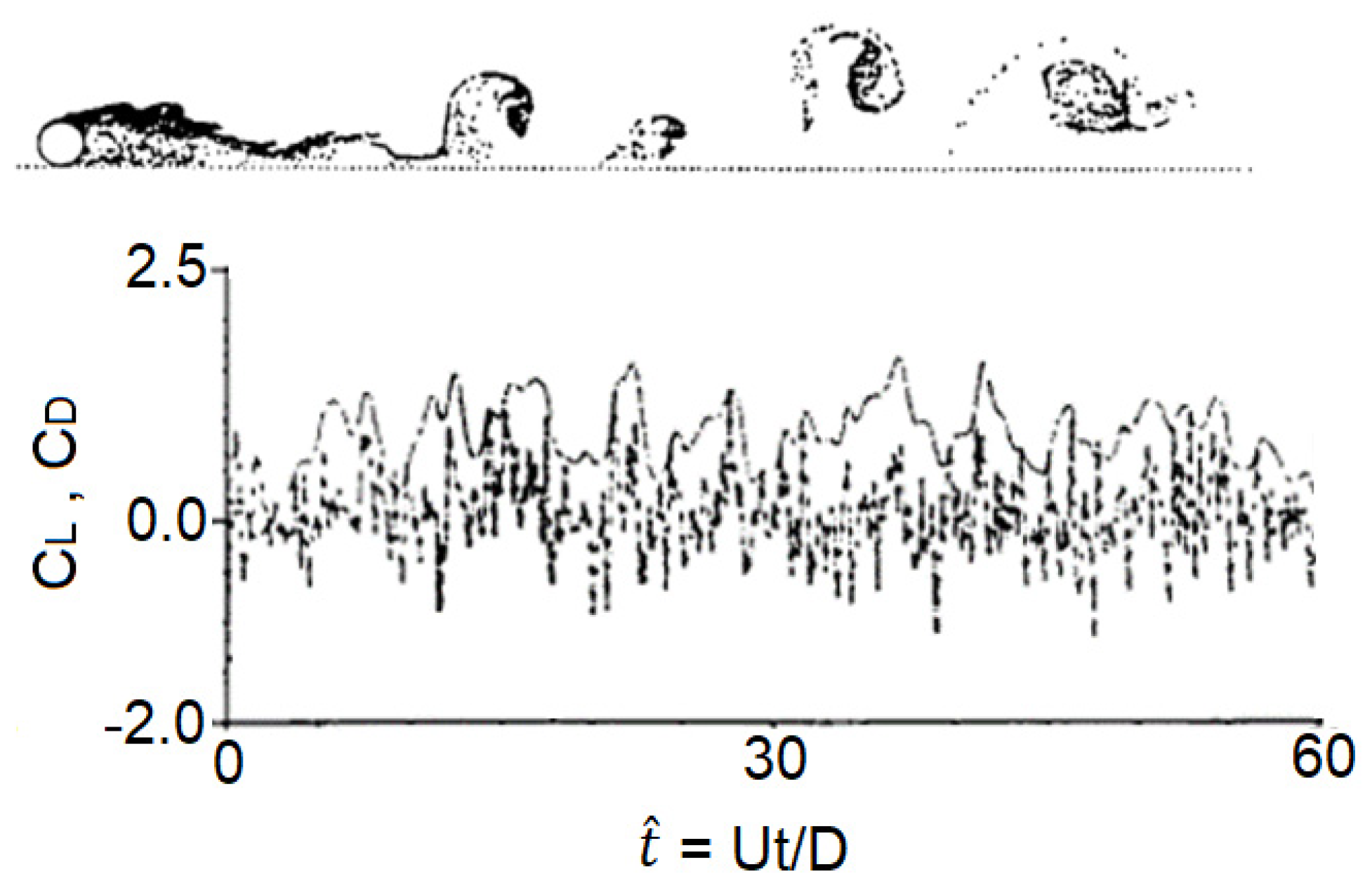
This affects the formation region which is lengthened to about eight times the cylinder diameter. Although there is no turbulence model applied in this study, numerically, the regular vortex shedding was still suppressed by the cancellation of the vortices shed from the lower part of the cylinder as they move closer than 0.05D from the wall, the minimum distance in which a vortex is still considered ‘alive’. The result for a gap ratio of 0.1D is presented in Figure 12. The loss of circulation due to the vortex cancellation is then compensated in the next calculation of the surface vorticity for the next time step. At this gap ratio, the mean value of the lift and drag coefficients are increased unrealistically, even though the suppressed oscillating flow pattern is achieved. This unrealistic result is attributed to the strong interaction between the closest elements of the cylinder and the wall, and the resultant interaction could not model the interaction between the wall and the cylinder boundary layer correctly.
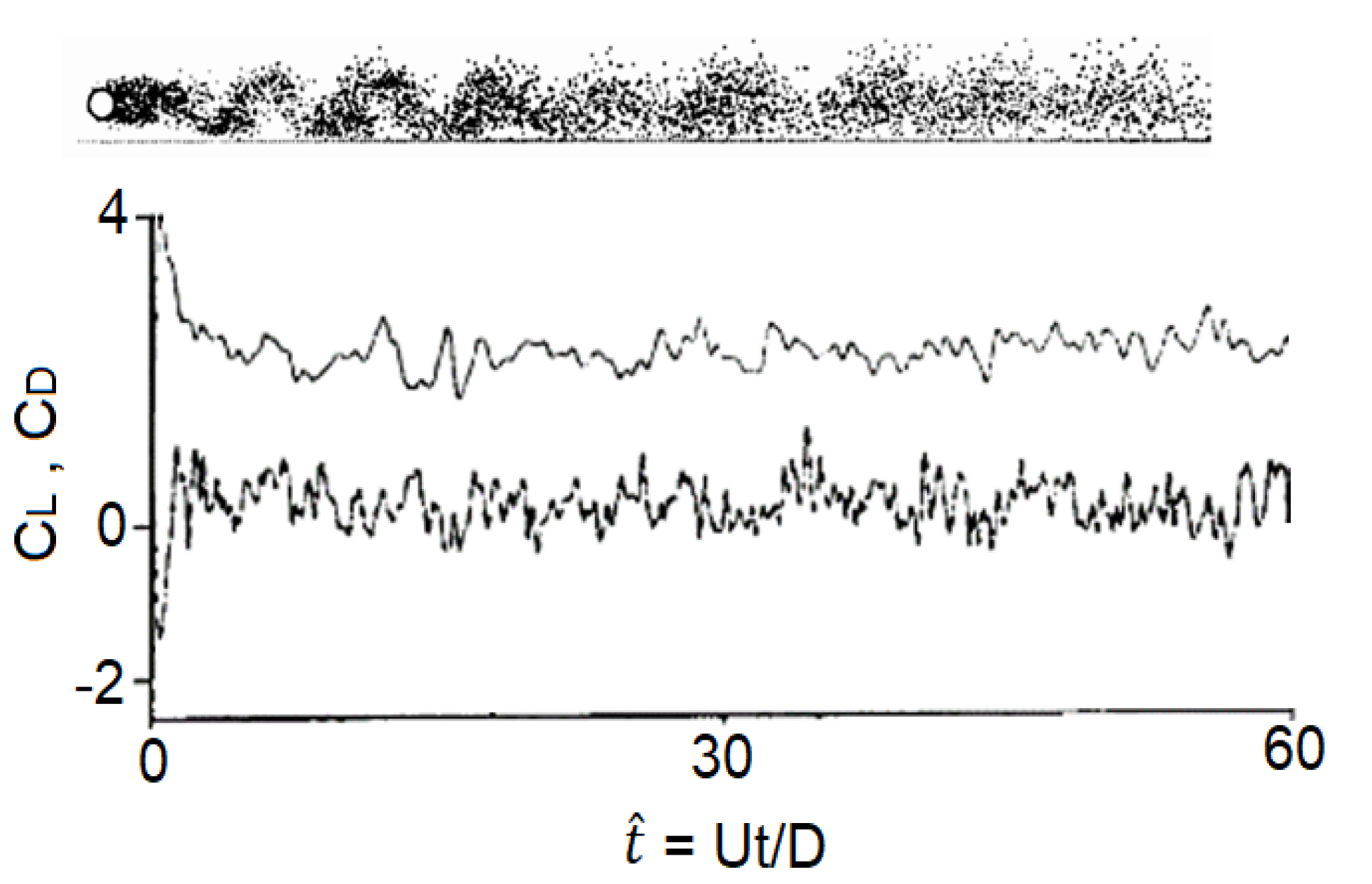
The effects of the Reynolds number at a fixed gap ratio value of G/D = 1 are also investigated in this study and the results are presented in Figure 12, Figure 13, Figure 14 and Figure 15. At Reynolds number 100, the resolution of the flow pattern is not as high as anticipated due to the dominant influence of the Random Walk diffusion scheme. The drag coefficient is found to be around 2.3 and the mean value of the lift coefficient is around 0.4.
The value of the Strouhal number is difficult to ascertain due to the numerical noise. This shows that the presence of the wall causes the drag coefficient to increase by about 10% and this can be attributed to the higher velocity in the gap region, which in turn creates stronger vortices that have a greater influence on the drag characteristics of the cylinder when they accumulate and interact in the formation region. At a higher Reynolds number of 500, a better picture of the flow pattern is observed; this is also reflected in the increased definition of the lift coefficient, as shown in Figure 12.
The drag coefficient is reduced to around 1.9, which is slightly higher than the value of the isolated cylinder, while the mean value of the lift coefficient is around 0.3. The mean maximum value of the lift coefficient is around 0.8 with the Strouhal number value around 0.17. The drag coefficient continuously decreases at higher Reynolds numbers, greater than 1000, with values of around 1.6, 1.2 and 1.15, as shown in Figure 13, Figure 14 and Figure 15, respectively. The mean maximum lift coefficient increases to around 0.9 with the Strouhal number reaching 0.2, which are both around the value obtained for the isolated cylinder. A summary of the results for the force coefficients of a cylinder placed at various distances from the wall with a Reynolds number of 100,000 is shown in Table 2 below. The effect of the variation of the Reynolds number, in the range of 100 to 50,000, on the force coefficients at a gap ratio value of G/D = 1 is shown in Table 3.
In a constant flow regime, the upper separation point moves upwards by decreasing G/D, indicating that the separation angle, θ, decreases too. This can be described by the growing stream-wise pressure gradient induced by the gap flow [4].

4.2. Oscillatory Flow

The range of validity of the present model and the parameters defining it were discussed. The object of this section of the study is to examine the influence of the proximity of a cylinder to a plane surface bounding an oscillatory flow in the context of the limitations of the model used.
It was concluded that the present model could only produce results in reasonable agreement with the experimental results when the β value ( K c R e ) 1 / 2 lies in a range in which the ‘boundary layer thickness’ is around half to twice the length of the local element. The Keulegan–Carpenter number Kc is a parameter which shows the scale of the motion of the water particles relative to the cylinder diameter. It is necessary to investigate the behavior of the present model upon the variation of the diameter of the first ring with respect to the cylinder diameter and also of the time step.
Using the cylinder parameters (the number of elements Ne is 64, the time step Δt is 0.15, and vortices are released from the first ring out) the hydrodynamic behavior of the cylinder and its flow pattern at the Keulegan–Carpenter number K c = U T D   of 40, with gap ratios G/D of 2, 1, 0.5, 0.2, 0.1, and values of Reynolds number Re of 25,000, 50,000, 75,000, 100,000, are investigated.   u is the maximum velocity and the equation is u = u cos ( 2 π t T ) .
At the first gap ratio of G/D = 2, the flow pattern and the force coefficient are displayed in Figure 16. At t ^   = 22.5, the pseudo-Karman vortex type of flow is produced behind the cylinder. The influence of the wall that is expressed in the suppression of the vortex street is not apparent in the region close to the cylinder. This is mainly due to the relatively wide gap between the cylinder and the wall. When the flow is reversed, more vortices will move closer again to the cylinder, compared to that of the isolated cylinder, as they are unable to spread in a downward direction due to the presence of the wall. It is seen that the vortices approach the wall tangentially. However, any vortices crossing the wall have been removed.
The in-line force coefficient is only slightly less than the experiment results by about 5% [19,20]. The values for the drag and inertia coefficients of the experimental results are 1.43 and 1.17, while those obtained from the present study are 1.56 and 1.89, respectively.
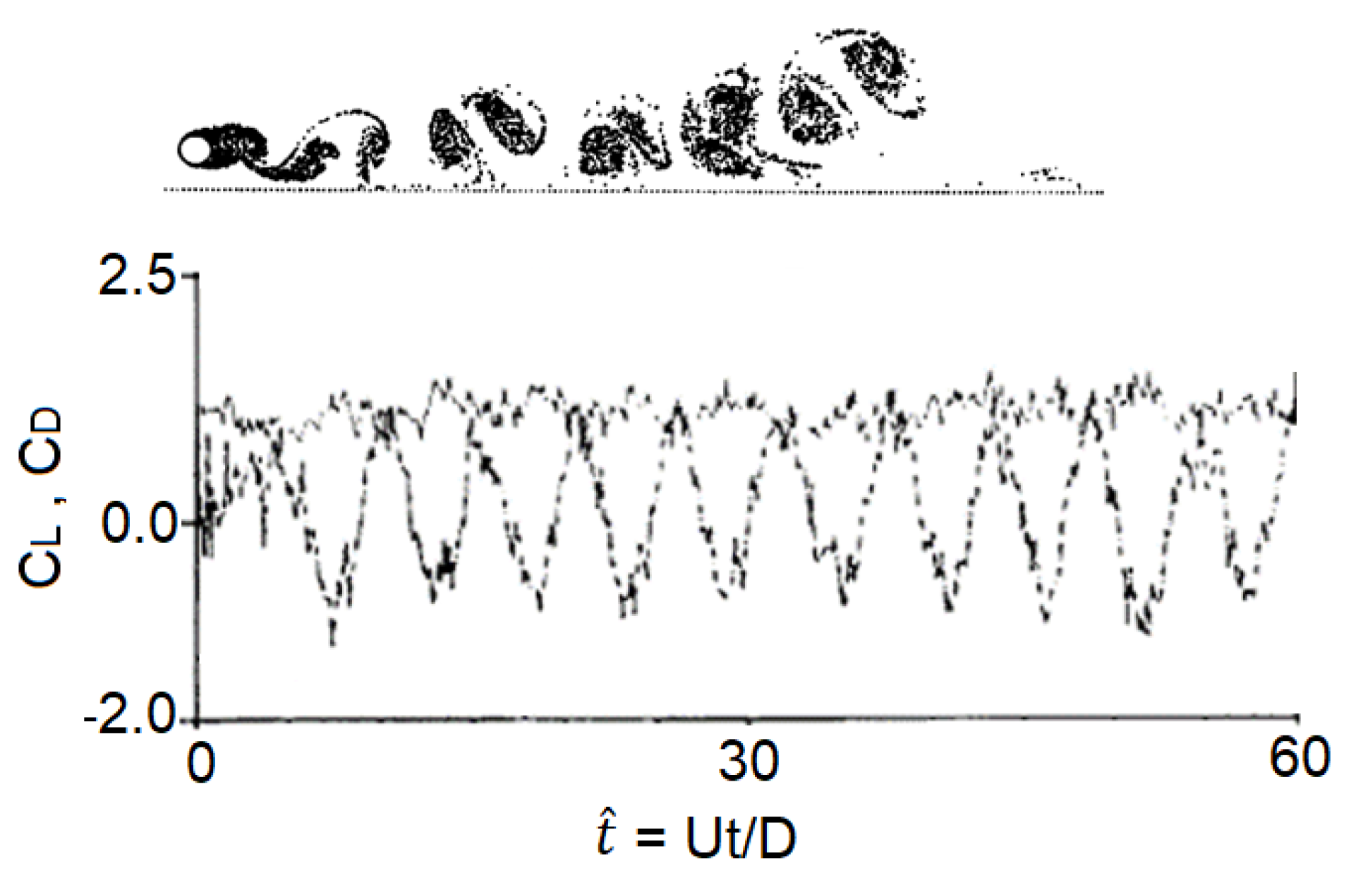
At the lower gap ratio of G/D = 1, the pseudo-Karman vortex street type flow also appeared behind the cylinder. The stronger influence of the wall is reflected in a more curved shape of the vortex street when it approaches the wall. This can also be seen in the higher amplitude of the drag coefficient which increases by about 5% compared to the previous case. As also displayed in Figure 17, the amplitude of the drag coefficient is higher than the experimental results by about 4% [20], whereas the phase is in quite good agreement.
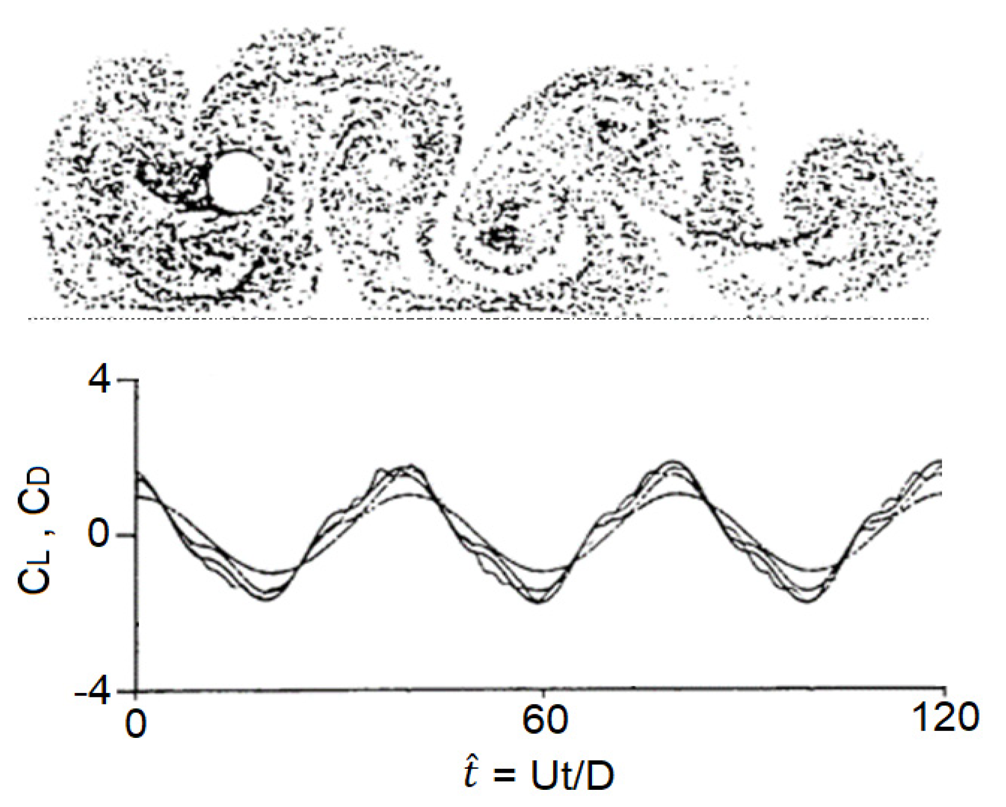
As the gap ratio is reduced to G/D = 0.5, the difference in the amplitude of the drag coefficient compared to that of the experimental results is narrowed to about 3% and the phase of the flows are again in good agreement, as shown in Figure 18. The flow pattern still has similarities with the unbounded oscillatory flow, but the trend of a deflected wake on the wall side of the cylinder is increasingly pronounced.
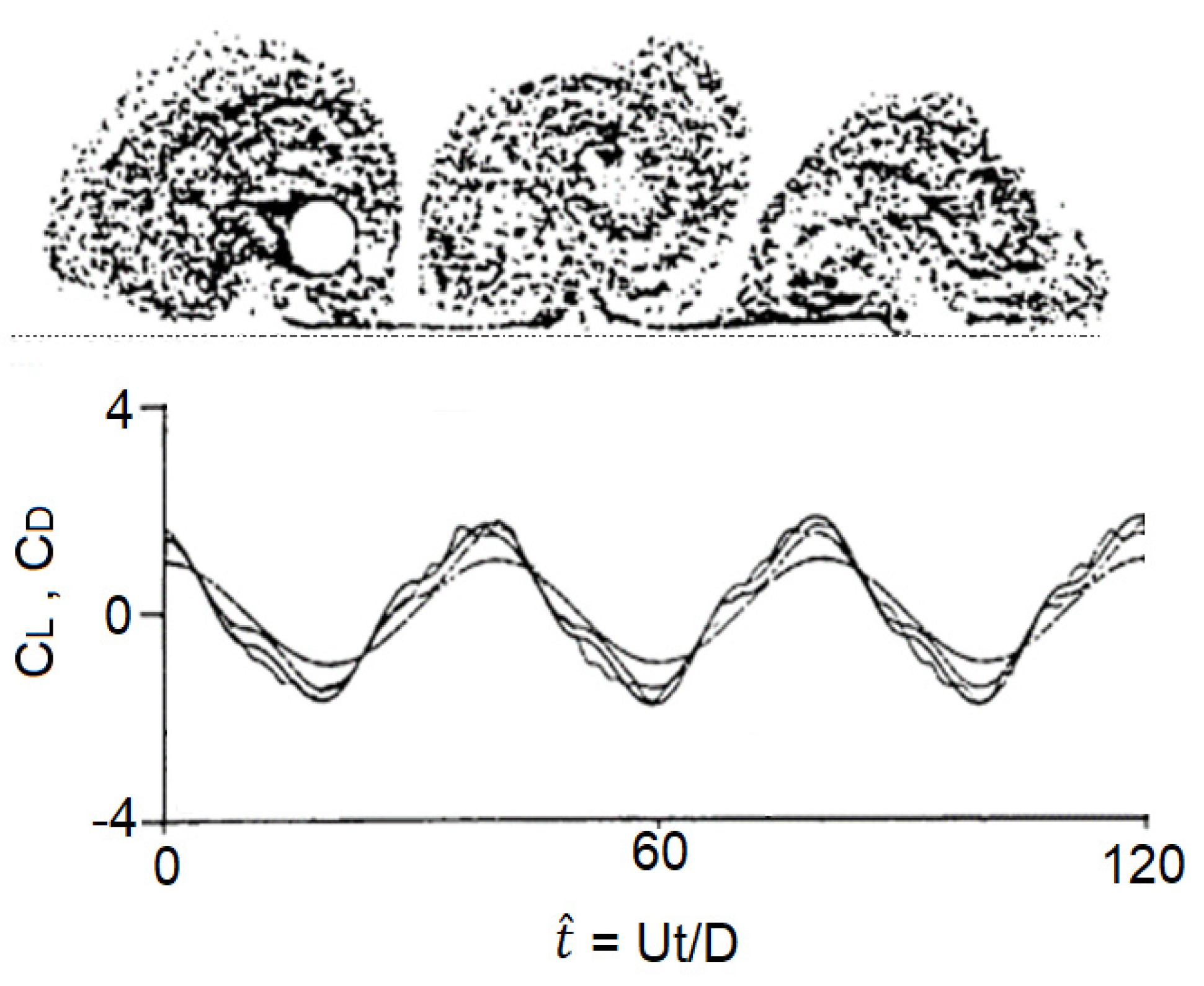
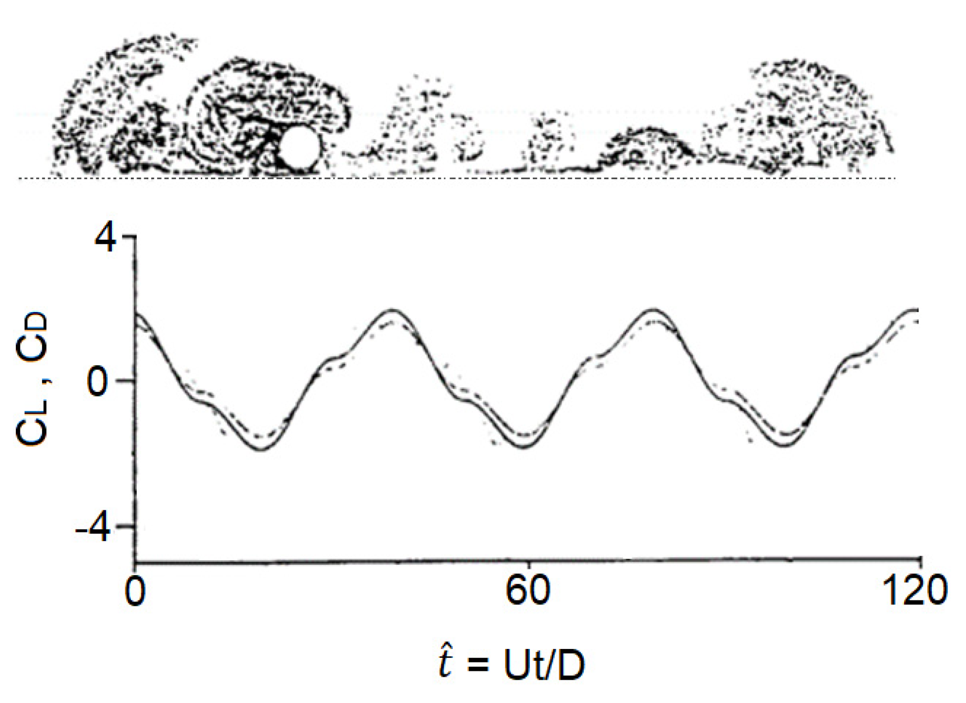
The flow becomes even more distorted when the cylinder is placed closer with G/D = 0.2. A drag coefficient with amplitude around 1.9 is produced, which is within 2% of the experimental results, as shown in Figure 19. As reported by a number of studies [21,22], when the gap ratio is close to the wall, the turbulent boundary layers created on the wall and cylinder surface and their interaction causes the drag coefficient of the cylinder to drop to about 1.3.
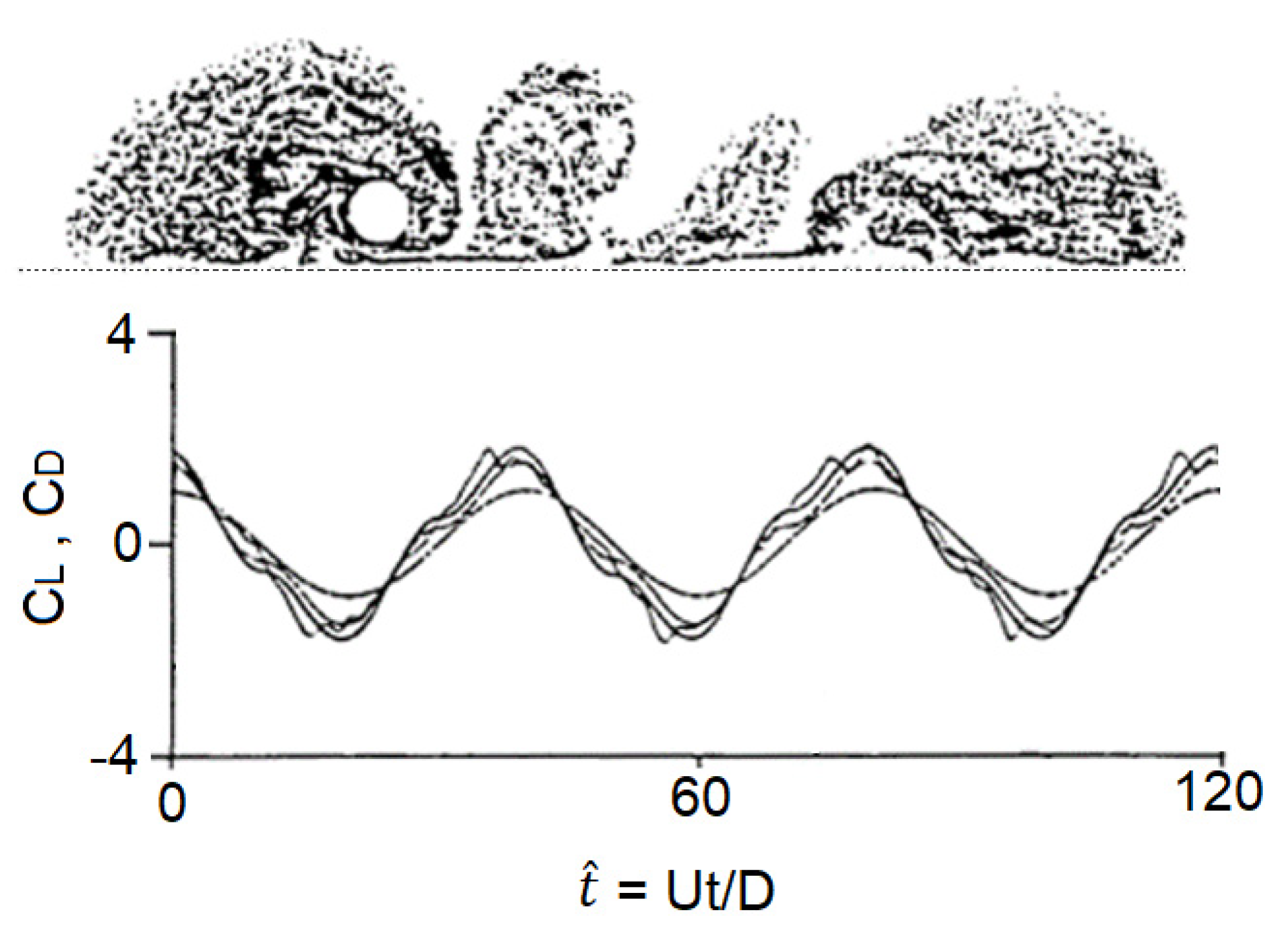
As has been discussed already, the present study model cannot reproduce the effects, and although the results are surprisingly close to experimental results for the larger gap ratios, for G/D less than 0.2, they become increasingly unrealistic, as shown in 
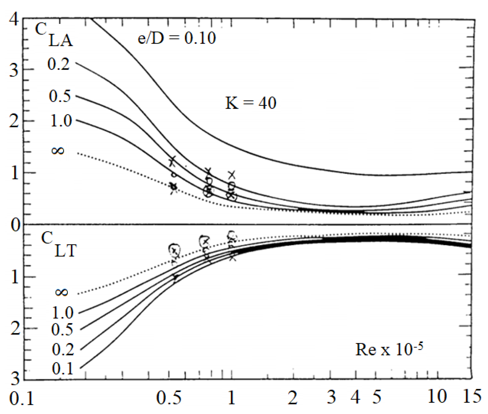
Figure 20. The effect of the wall proximity on the lift coefficient of a circular cylinder is shown in Figure 21. CLA and CLT are the mean peak of the lift coefficients in directions against and towards the wall, respectively.
The effect of wall proximity becomes insignificant, however, when the turbulence either in the form of organized motion (namely, vortex shedding in the case of a wall-free cylinder) or in the form of disorganized wake flow in the case of a wall-mounted cylinder, is considered [7].

5. Conclusions

Another use of the discrete vortex model for investigating the flow around a single cylinder placed near a plane wall in unidirectional and oscillatory flow has been presented. In this model, the size of the wall source element is equal to the size of the rectangular grid segment. Two different kinds of boundary conditions are solved simultaneously on the cylinder, with zero tangential velocity, and on the wall, with zero normal velocity. The influence of the vortices on the cylinder is computed using the polar grid node while that of the wall is computed using the rectangular grid. In other words, there is no direct calculation of the interaction between the wall and the active polar grid nodes. This grid strategy was chosen in an attempt to achieve a satisfactory interaction between the cylinder, shed vortices and the wall sources. In oscillatory flows, an increase in the mean peak drag coefficient compared to that of an isolated cylinder was also detected. In the case of a cylinder placed near a plane wall in unidirectional flows, the positive mean lift coefficient is generally predicted well. However, when the gap is less than 0.1 D the algorithm fails to produce realistic results for the force coefficient since there is no exact boundary layer program in the model.

Author Contributions

Conceptualization, W.W.; formal analysis, W.W., E.M.W. and M.S.; methodology, W.W., E.M.W. and M.S.; supervision, W.W.; validation, W.W., E.M.W. and M.S.; writing, W.W., E.M.W. and M.S. All authors have read and agreed to the published version of the manuscript.

Funding

This research was financially supported by the Ministry of Education and Culture of Indonesia.

Institutional Review Board Statement

Not applicable.

Informed Consent Statement

Not applicable.

Data Availability Statement

Not applicable.

Acknowledgments

The authors would like to thank Martin J. Downie for his patient supervision. Thanks also to Bilal Pradanahadi for typing this paper. Gratitude is also given to Diar and Frea M. Wardhana for their patience and help during the research.

Conflicts of Interest

The authors declare no conflict of interest.

References

  1. Engelbreth, K.I. Viscous Flow around a Circular Cylinder Near a Plane Wall. Master’s Thesis, Department of Marine Technology, Norwegian University of Science and Technology, Trondheim, Norway, 2011. [Google Scholar]
  2. Chen, L.F.; Wu, G.X. Boundary Shear Flow Past a Cylinder Near a Wall. J. Appl. Ocean Res. 2019, 92, 101923. [Google Scholar] [CrossRef]
  3. Laroussi, M. Vortex Shedding for Flow Past Circular Cylinder: Effects of Initial Conditions. Univ. J. Fluid Mech. 2015, 3, 19–32. [Google Scholar]
  4. Salehi, M.A.; Mazaheri, S.; Kazeminezhad, M.H. Study of Flow Characteristics around a Near-Wall Circular Cylinder Subjected to a Steady Cross-Flow. Int. J. Coast. Offshore Eng. 2018, 1, 45–55. [Google Scholar] [CrossRef] [Green Version]
  5. Prsic, M.A.; Ong, M.C.; Pettersen, B.; Myrhaug, D. Large Eddy Simulation of Flow around a Circular Cylinder Close to a Flat Seabed. J. Mar. Struct. 2016, 46, 127–148. [Google Scholar] [CrossRef] [Green Version]
  6. Li, Z.; Yao, W.; Yang, K.; Jaiman, R.K.; Khoo, B.C. On the Vortex-Induced Oscillations of a Freely vibrating cylinder in the Vicinity of a Stationary Plane Wall. J. Fluids Struct. 2016, 65, 495–526. [Google Scholar] [CrossRef]
  7. Kozakiewicz, A.; Sumer, B.M.; Fredsoe, J. Spanwise Correlation on a Vibrating Cylinder Near a Wall in Oscillatory Flows. J. Fluids Struct. 1992, 6, 371–392. [Google Scholar] [CrossRef]
  8. Murray, B.A. Hydrodynamic Loading due to Appurtenances on Jacket Structures. Ph.D. Thesis, Newcastle University, Newcastle upon Tyne, UK, 1992. [Google Scholar]
  9. Wardhana, W. Prediction of 2D Separated Flows about a Circular Cylinder in the Presence of Boundaries. Ph.D. Thesis, Newcastle University, Newcastle Upon Tyne, UK, 1995. [Google Scholar]
  10. Yamamoto, T.; Nath, J.H.; Slotta, L.S. Wave Forces on Cylinders Near a Plane Boundary. J. Waterw. Harb. Coast. Eng. Div. 1974, 100, 345–359. [Google Scholar] [CrossRef]
  11. Downie, M.J. An Inviscid Model for the Fluid Forces Induced by Vortex Shedding from a Circular Cylinder. Ph.D. Thesis, Royal Military College of Science, Shrivenham, UK, 1981. [Google Scholar]
  12. Bearman, P.W.; Zdravkovich, M.M. Flow around a Circular Cylinder Near a Plane Boundary. J. Fluid Mech. 1978, 89, 33–47. [Google Scholar] [CrossRef]
  13. Chorin, A.J. Numerical Study of Slightly Viscous Flow. J. Fluid Mech. 1973, 57, 785–796. [Google Scholar] [CrossRef]
  14. Chorin, A.J. Vortex Sheet Aproximation of Boundary Layers. J. Comput. Phys. 1978, 27, 428–442. [Google Scholar] [CrossRef] [Green Version]
  15. Lewis, R.I. Vortex Element Methods for Fluid Dynamic Analysis of Engineering Systems; Cambridge University Press: Cambridge, UK, 1991. [Google Scholar]
  16. Lewis, R.I.; Porthouse, D.T.C. Recent Advances in the Theoretical Simulation of Real Fluid Flows; North East Coast Institute of Engineers and Shipbuilders: Newcastle-on-Tyne, UK, 1983; Volume 99. [Google Scholar]
  17. Angrilli, F.; Bergamaschi, S.; Cossalter, V. Investigation of Wall Induced Modifications to Vortex Shedding from a Circular Cylinder. J. Fluid Eng. 1982, 104, 518–522. [Google Scholar] [CrossRef]
  18. Price, S.J.; Sumner, D.; Smith, J.G.; Leong, K.; Paidoussis, M.P. Flow Visualization Around Circular Cylinder Near to a Plane Wall. J. Fluids Struct. 2002, 16, 175–191. [Google Scholar] [CrossRef]
  19. Sarpkaya, T. Forces on Cylinders and Spheres in a Sinusoidally Oscillating Fluid. J. Appl. Mech. 1975, 42, 32–37. [Google Scholar] [CrossRef]
  20. Sarpkaya, T. In-Line and Transverse Forces on Cylinders in Oscillatory Flows. In Proceedings of the Offshore Technology Conference, Houston, TA, USA, 2 May 1976. [Google Scholar]
  21. Graham, J.M.R. Computation of Viscous Separated Flow Using a Particle Method. In Proceedings of the Conference on Numerical Methods for Fluid Dynamics, Oxford, UK, 21–24 March 1988. [Google Scholar]
  22. Bearman, P.W.; Wadcock, A.J. The Interaction between a Pair of Circular Cylinders Normal to a Stream. J. Fluid Mech. 1973, 61, 499–511. [Google Scholar] [CrossRef]
Figure 1. The overlapping grid system.
Fluids 06 00211 g001
Figure 2. Effect of wall length to the cylinder.
Fluids 06 00211 g002
Figure 3. The flow pattern of a cylinder near a wall, G/D = 0; G/D = 0,2; G/D = 0.4, copyright [12].
Fluids 06 00211 g003
Figure 4. Vortex shedding frequency vs. wall distances.
Fluids 06 00211 g004
Figure 5. The flow pattern at t ^ = 1 and 5 at G/D = 0.5.
Fluids 06 00211 g005
Figure 6. The flow pattern and force coefficients for G/D = 2 and Re = 100,000.
Fluids 06 00211 g006
Figure 7. The flow pattern and force coefficients for G/D = 1.5 and Re = 100,000.
Fluids 06 00211 g007
Figure 8. The flow pattern and force coefficients for G/D = 1 and Re = 100,000.
Fluids 06 00211 g008
Figure 9. The flow pattern and force coefficients for G/D = 0.5 and Re = 100,000.
Fluids 06 00211 g009
Figure 10. The flow pattern and force coefficients for G/D = 0.25 and Re = 100,000.
Fluids 06 00211 g010
Figure 11. The flow pattern and force coefficients for G/D = 0.1 and Re = 100,000.
Fluids 06 00211 g011
Figure 12. The flow pattern and force coefficients for G/D = 1 and Re = 100.
Fluids 06 00211 g012
Figure 13. The flow pattern and force coefficients for G/D = 1 and Re = 500.
Fluids 06 00211 g013
Figure 14. The flow pattern and force coefficients for G/D = 1 and Re = 1000.
Fluids 06 00211 g014
Figure 15. The flow pattern and force coefficients for G/D = 1 and Re = 10,000.
Fluids 06 00211 g015
Figure 16. The flow pattern at t = 120, and the force coefficients for G/D = 2, Kc = 40 and Re = 25,000.
Fluids 06 00211 g016
Figure 17. The flow pattern at t = 120, and the force coefficients for G/D = 1, Kc = 40 and Re = 25,000.
Fluids 06 00211 g017
Figure 18. The flow pattern at t = 120, and the force coefficients for G/D = 0.5, Kc = 40 and Re = 25,000.
Fluids 06 00211 g018
Figure 19. The flow pattern at t = 120, and the force coefficients for G/D = 0.2, Kc = 40 and Re = 25,000.
Fluids 06 00211 g019
Figure 20. The flow pattern at t = 120, and the force coefficients for G/D = 0.1, Kc = 40 and Re = 25,000.
Fluids 06 00211 g020
Figure 21. The mean peak of the lift coefficient vs. Reynolds numbers.
Fluids 06 00211 g021
Table 1. The CPU time percentage of the algorithm.
Section NumberPurpose of SectionCPU Time
1Input/Output1.59
2Define Grid0
3Calculate Nodal Velocity73.97
4Calculate Vortex Velocity2.38
5Vortex Displacement1.6
6Distribute Circulation1.1
7Calculate Surface Velocity16.03
8Calculate Forces0.01
Table 2. Results for Reynolds number 100.
Gap RatioDrag CoefficientLift Coefficient
G/DCDCL
0.1unrealisticunrealistic
0.250.751.45
0.50.411.2
0.750.311.17
10.251.15
1.50.221.13
20.151.13
Table 3. Results for G/D = 1.
Reynolds NumberLift CoefficientDrag Coefficient
ReCdCL
1000.42.3
5000.31.9
10000.31.6
10,0000.251.2
100,0000.151.15
Publisher’s Note: MDPI stays neutral with regard to jurisdictional claims in published maps and institutional affiliations.

