Low-Noise Synthetic Turbulence Tailored to Lateral Periodic Boundary Conditions

Abstract

The present work is dedicated to turbulence synthesis tailored to lateral periodic boundary conditions for direct noise computations through compressible large eddy simulations. Synthetic turbulence can be essential for aeroacoustic applications when computing airfoil turbulent inflow noise or for accurately capturing the behavior of boundary layers. This behavior determines both trailing edge noise and complex flow structures such as laminar separation bubbles. For airfoil simulation purposes, spanwise periodic boundary conditions are usually considered. If synthetic perturbations are injected without observing the periodicity rule, strong spurious pressure waves are emitted and pollute the entire computational domain. In this work, the random Fourier modes method for turbulence generation is adapted in order to respect the spanwise periodicity constraint right at the computational domain inlet. This approach does not affect the turbulence properties such as the spectral shape and the turbulent kinetic energy decay. Since the emphasis is put on the generation and convection of the turbulence, only the turbulence convection region between the inlet and the airfoil is considered in this paper, without the airfoil. Two geometrical configurations are tested: the first one is a simple box with a constant mesh size, and the second one concentrates the fine cells on the area in front of the airfoil. In the second configuration, the computational cost is reduced by up to 25%, but more spurious noise is present because of interpolation areas between different grids using the Chimera method. Finally, the results’ reproducibility is assessed using different turbulence realizations.

1. Introduction

Low-Reynolds number (i.e., $Re\le 5\times {10}^5$ [1]) aerodynamic applications such as small wind turbines or drones appear to be more and more present for civil or military use. The flow on blades can be subject to complex phenomena such as laminar boundary layer separation, transition towards turbulence, boundary layer reattachment or even stall [1]. Boundary layer separation and reattachment form the well-known laminar separation bubble (LSB) that can lead to wing stall when the LSB bursts at high angles of attack. In this situation, the underlying mechanisms still need to be understood [2,3]. Furthermore, the noise emitted by drones at low Reynolds numbers is a subject of growing interest [4,5]. It is also the case for higher-Reynolds number applications such as full-scale wind turbines [6].

For both low- and high-Reynolds number applications, inflow turbulence is of significant importance. In the case of a full-scale wind turbine, inflow turbulence is responsible for broadband low-frequency noise [7,8]. For low-Reynolds number applications, inflow turbulence not only affects emitted noise but also strongly impacts the aerodynamics. Indeed, it is experimentally suggested that the transition towards turbulence of the LSB on an airfoil, its length and its burst are highly affected by inflow perturbations [2,3]. The effect of inflow turbulence on the LSB separation, transition and reattachment points has also been numerically studied using different turbulent intensities or integral length scales. For example, Hosseinverdi et al. [9] generated an LSB on a flat plate and injected turbulence built with Fourier modes, while Schmidt et al. [10] injected turbulence based on a modified digital filter approach to disturb an LSB present on an SD7003 airfoil.

For acoustic predictions or LSB insights, numerical simulations such as large eddy simulations (LES) are a good compromise between resolution and computational cost. Previous studies showed the importance of generating realistic inflow turbulence in simulations. There are still two major challenges concerning synthetic turbulence. The first one is that most methods are unable to accurately reproduce experimental turbulence high-order statistics at the computational domain inlet [11]. The second challenge concerns direct noise computation (DNC) which requires that synthetic turbulence methods generate low levels of spurious noise [12].

The different categories and methods of synthetic inflow turbulence were reviewed in Dhamankar et al. [11]. While library-based turbulence methods are efficient in terms of statistics’ reproducibility, they can only be used for specific applications and can be very expensive. The recycling methods avoid a long turbulence adaptation distance but present the drawback of generating spurious modes in the flow [11]. Furthermore, these methods exploit turbulent boundary layer similarity laws for rescaling. The last category of methods is based on synthetic turbulence generators and includes several approaches. These approaches are still missing correct third-order turbulence statistics but have the advantage of being directly embedded in solvers, without running any other simulation in parallel. Kraichnan [13] first proposed a spectral approach with a Gaussian distribution for the mode amplitudes. Smirnov et al. [14] and Batten et al. [15] extended this work by adding anisotropy and inhomogeneity properties. Among others, Karweit et al. [16] or Bechara et al. [17] generated isotropic turbulent fields with a deterministic energy distribution using a theoretical spectrum. This method, called random Fourier modes (RFM), consists of building turbulence with a realistic prescribed energy spectrum and has the advantage of naturally producing an incompressible velocity field, in order to synthesize low-noise turbulence. Sescu et al. [18] later showed that a synchronicity between the turbulence perturbations and the mean flow is needed to avoid the generation of spurious vorticity waves. The RFM method was used with two-dimensional structures to compute the leading edge noise of wavy airfoils with the Euler equations in Clair et al. [19].

The synthetic eddy method (SEM) [20] is another technique to produce turbulence and was initially used for channel flow incompressible simulations. This method has been modified to introduce realistic scale inhomogeneities in a flat-plate turbulent boundary layer in the wall-normal direction [21], and to reduce spurious noise emission [18] by making the resulting fluctuating velocity field incompressible. Later, Kim and Haeri [22] extended this work to retrieve a von Kármán spectrum by optimizing the method with constraint parameters. They applied it to turbulence interaction noise on a wavy airfoil with the Euler equations.

Another group of methods for the generation of inflow perturbations was introduced by Klein et al. [23]. With an incompressible solver, the authors used white noise digital filtering to create turbulent fields. In [23], these perturbations were employed to study the influence of the integral length scale, the mean flow velocity profile and the turbulent intensity on plane jets and on the interface of a water film ejected into air. Later, Ewert [24] introduced the random particle mesh method (RPM) to obtain a solenoidal velocity field using digital filtering on a fluctuating vector stream function. He successfully applied this method to compute slat noise. At the same time, Xie et al. [25] improved the computational efficiency of the digital filtering method. They applied it to a plane channel flow and to an urban-type configuration, using an incompressible solver. Kim et al. [26] then modified this last method by adding a mass flux correction at the inlet and by making the velocity field solenoidal through the Pressure-Implicit with Splitting of Operators (PISO) algorithm corrector steps. This allowed them to delete the spurious pressure waves by making the turbulence generation method consistent with the incompressible solver even if the adaptation distance increased. Kim and Xie [27] used this turbulence generation method to study the effect of freestream turbulence on a NACA0012 airfoil dynamic stall. They worked in the context of a small or medium-size wind turbine by choosing a chord-based Reynolds number equal to $1.35\times {10}^5$. Recently, Gea-Aguilera et al. [28] extended the RPM method by replacing the white noise field by a scalar randomly taking the value $\pm 1$ for each synthetic eddy, which resulted in a computational cost improvement. This method is called advanced digital filtering and was used to compute airfoil leading edge noise by solving the linearized Euler equations.

For DNC, silent synthetic turbulence is sought but is still difficult to obtain. Indeed, in compressible codes, the velocity is often prescribed at the inlet without the thermodynamic variables, that leads the code to adapt the flow field and to generate undesired pressure fluctuations, as explained in Gloerfelt and Robinet [12]. Another source of spurious noise is found in airfoil aeroacoustic simulations. Indeed, spanwise periodic boundary conditions are commonly used to limit the computational cost, but the inflow turbulence does not necessarily respect this condition, that leads the solver to generate undesired pressure waves. Kim and Haeri [22] solved this problem for their modified SEM by duplicating the generated turbulence virtual boxes on each side of the span limits. Clair et al. [19] used in their Euler-based solver a two-dimensional RFM method built with a wavenumber component in the periodic direction equal to zero. Indeed, at a low Mach number, the wavenumbers with a non-zero component in the spanwise direction have a negligible impact on the far-field noise radiated in the mid-span plane, if the airfoil span is at least three times greater than its chord [19,29]. However, when the Mach number increases, the modes whose wavenumber component in the spanwise direction is non-zero become important for the far-field noise calculation.

The aim of the present work is to eliminate the spurious noise triggered by the spanwise non-periodicity of three-dimensional synthetic turbulence. In this paper, synthetic turbulence is generated using the RFM method inside Code_Safari [30], an EDF R&D code. It enables one to carry out relaxation filtering LES [31,32] using high-order finite-difference schemes and selective filters. In the first step, the RFM method is used inside Code_Safari to generate divergence-free turbulence at the inlet. This method was especially chosen because of its straightforward capability to impose a desired turbulent spectrum, its simplicity of implementation and its ability to synchronize the turbulent fluctuations with the mean flow [18]. In the second step, an extension of the RFM method called RFM-P is proposed. The RFM-P approach forces the random Fourier modes to respect the periodicity condition in the lateral direction, meaning that less spurious noise is generated. In the context of airfoil simulations, the lateral direction is chosen along the span.

This paper is organized as follows. First, the flow solver and the synthetic turbulence methods are described in Section 2. Then, spatially decaying homogeneous isotropic turbulence (HIT) simulations using both the RFM method and the RFM-P extension are detailed in Section 3. Two geometrical configurations are proposed. The first one is used for a reference calculation, and the second one is built for the purpose of computational cost reduction. Since this study focuses on the turbulence generation and convection, the airfoil is not included in the present computations. Only the region between the inlet and a virtual airfoil is considered. The turbulence properties are analyzed to determine the RFM-P performance compared to the RFM one.

2. Numerical Methods: Flow Solver and Inflow Synthetic Turbulence

2.1. Flow Solver

In this work, an EDF R&D finite-difference code, called Code_Safari [30], is used to carry out DNC through LES. Considering a Newtonian fluid and a Cartesian mesh $\underline{x}=$ (x, y, z) transformed into a curvilinear one $\underline{\xi }=$ ($\xi$, $\eta$, $\zeta$), the compressible equations to be solved are

$$\frac{\partial }{\partial t}\widehat{\mathbf{U}}+\frac{\partial }{\partial \xi }({\mathbf{F}}_{\xi }-{\mathbf{F}}_{\xi }^{\nu })+\frac{\partial }{\partial \eta }({\mathbf{F}}_{\eta }-{\mathbf{F}}_{\eta }^{\nu })+\frac{\partial }{\partial \zeta }({\mathbf{F}}_{\zeta }-{\mathbf{F}}_{\zeta }^{\nu })=0,$$

(1)

where t is the time, $\widehat{\mathbf{U}}=\mathbf{U}/J$ with $\mathbf{U}={(\rho ,\rho \mathbf{u},\rho e)}^T$ the conservative variables vector and J is the curvilinear transformation matrix Jacobian. The density is $\rho$, $\mathbf{u}={(u,v,w)}^T$ denotes the velocity vector in the Cartesian coordinates, and e is the total specific energy. Here, the equation of state is assumed to be the ideal gas law. Non-viscous fluxes are ${\mathbf{F}}_{\xi }$, ${\mathbf{F}}_{\eta }$, ${\mathbf{F}}_{\zeta }$, while the viscous ones are ${\mathbf{F}}_{\xi }^{\nu }$, ${\mathbf{F}}_{\eta }^{\nu }$, ${\mathbf{F}}_{\zeta }^{\nu }$. Their expressions can be found in Daude et al. [30]. To avoid the dissipation and dispersion of acoustic waves, the spatial discretization is carried out by an optimized 4th-order 11-point scheme [33], and the time advancement is realized by an optimized 2nd-order 6-step Runge–Kutta scheme [33]. From the first to the third points in the orthogonal direction with respect to the boundaries, the Tam and Webb dispersion-relation-preserving (DRP) [34] backward scheme is used for the spatial discretization. For the fourth and the fifth points, the DRP centered scheme is chosen. The dissipation of the non-resolved scales and of the grid-to-grid oscillations is ensured by a 6th-order explicit selective filter optimized on 11 points instead of subgrid models [35]. In the orthogonal direction with respect to the boundaries, filters based on centered decreasing-order schemes are used for numerical robustness from the first to the fifth points. The DRP centered scheme is applied for the fourth and fifth points, and standard schemes are chosen from the first to the third points. In this paper, outflow boundary conditions designate the Bogey and Bailly boundary conditions [36].

The Tam and Dong inflow boundary conditions [37] are implemented on 5 points in order to minimize the spurious noise when an inlet disturbance is introduced [12]. These conditions are given by

$$\left(\frac{1}{V_g}\frac{\partial }{\partial t}+\frac{\partial }{\partial r}+\frac{1}{r}\right)\left[\begin{array}{c}{\rho }^{\prime }\\ \underline{u^{\prime }}\\ p^{\prime }\end{array}\right]=\left(\frac{1}{V_g}\frac{\partial }{\partial t}+\frac{\partial }{\partial r}+\frac{1}{r}\right)\left[\begin{array}{c}{\rho }_i^{\prime }\\ \underline{u_i^{\prime }}\\ p_i^{\prime }\end{array}\right],$$

(2)

where $p^{\prime }$ is the fluctuating pressure assumed equal to the acoustic pressure, ${\rho }^{\prime }$ and $\underline{u^{\prime }}$ are the fluctuations of density and velocity, r is the radius in the spherical coordinates, $V_g$ is the phase velocity and (${\rho }_i^{\prime }$, $\underline{u_i^{\prime }}$, $p_i^{\prime }$) are the desired fluctuating quantities at the inlet. In Equation (2), ${\rho }_i^{\prime }$ and $p_i^{\prime }$ are set to zero since their expressions are unknown, although this is a source of spurious noise, as noticed by Gloerfelt and Robinet [12]. As it will be seen in Section 2.2.1, $\underline{u_i^{\prime }}$ is analytically known so that the right-hand side term of Equation (2) can be semi-analytically computed before being introduced in the equation, the Jacobian matrix between the Cartesian and the curvilinear grid being numerically computed. Finally, Equation (2) is computed at each substep of the Runge–Kutta algorithm to reduce the emitted spurious noise [12,37].

Code_Safari is parallelized using the OpenMPI Message Passing Interface (MPI) library. Periodic boundary conditions are treated as simple MPI communications using ghost points. Overset meshes with 8th-order interpolation are built with Overture [38], developed in the Lawrence Livermore National Laboratory. Details about the computational platform and libraries are given in Section 3.1.4.

2.2. Inflow Synthetic Turbulence

This section describes the synthetic turbulence algorithms implemented in Code_Safari. Firstly, the classical random Fourier modes (RFM) method is described in Section 2.2.1. Secondly, the RFM-P extension is described in Section 2.2.2; it takes into account the lateral periodic boundary conditions when computing the turbulence wavenumbers.

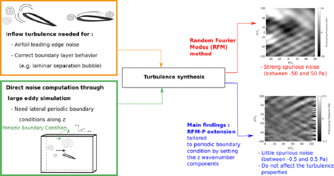
2.2.1. Classical Random Fourier Modes Method

The RFM method, based on [39], builds an incompressible turbulent velocity field by adding up N Fourier modes. Figure 1 schematically shows one mode and gives notations for the local spherical base ($\underline{e_{r_n}}$, $\underline{e_{{\theta }_n}}$, $\underline{e_{{\varphi }_n}}$).

The turbulent velocity field $\underline{u^{\prime }}$ can be written as

$$\underline{u^{\prime }}\left(\underline{x},t\right)=2\sum _{n=1}^N{\tilde{u}}_{n}cos\left(\underline{k_n}•\underline{x}+{\psi }_n-k_{nx}{U}_{x}t\right)\underline{{\sigma }_n},$$

(3)

where • denotes the scalar product, U_x is the mean flow field, ${\tilde{u}}_n$ is the nth mode amplitude, ${\psi }_n$ is the nth mode random phase, $\underline{{\sigma }_n}$ is the nth mode direction and $\underline{k_n}=\left(k_{nx},k_{ny},k_{nz}\right)$ is the nth mode wavenumber. To limit spurious noise, the incompressibility condition, $\underline{\nabla }•\underline{u^{\prime }} = 0$ is used, that leads to

$$\underline{k_n}•\underline{{\sigma }_n}=0.$$

(4)

Thus, the vector $\underline{{\sigma }_n}$ must be in the ($\underline{e_{{\theta }_n}}$, $\underline{e_{{\varphi }_n}}$) plane. Furthermore, Kim and Haeri [22] and Sescu and Hixon [18] showed that the mean flow and the disturbances must be synchronized to generate minimum spurious noise. This condition means that the angular frequency of the disturbance must be written as $\underline{k_n}•\underline{U}$, as it is written in Equation (3). Other details about the RFM method can be found in Appendix A. The RFM method generates a frozen divergence-free isotropic homogeneous turbulence with imposed turbulent kinetic energy $k_t$ and a longitudinal integral length scale ${\mathsf{\Lambda }}_f$. The chosen spectrum is the modified von Kármán one [17], given by Equation (A6). The wavenumber amplitudes are logarithmically distributed, and the wavenumber components are randomly computed using the spherical coordinate system angles, as seen in Appendix A.

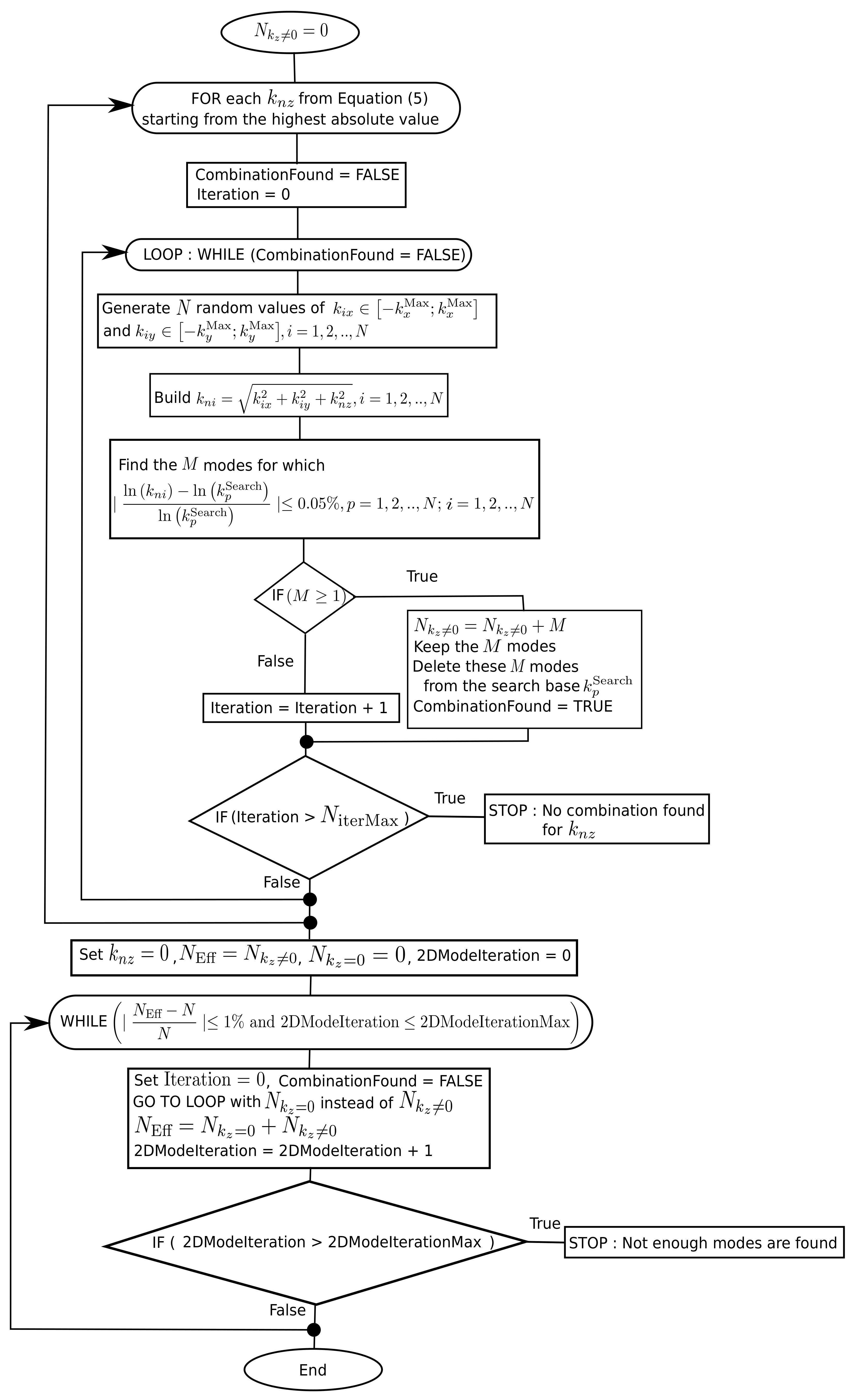
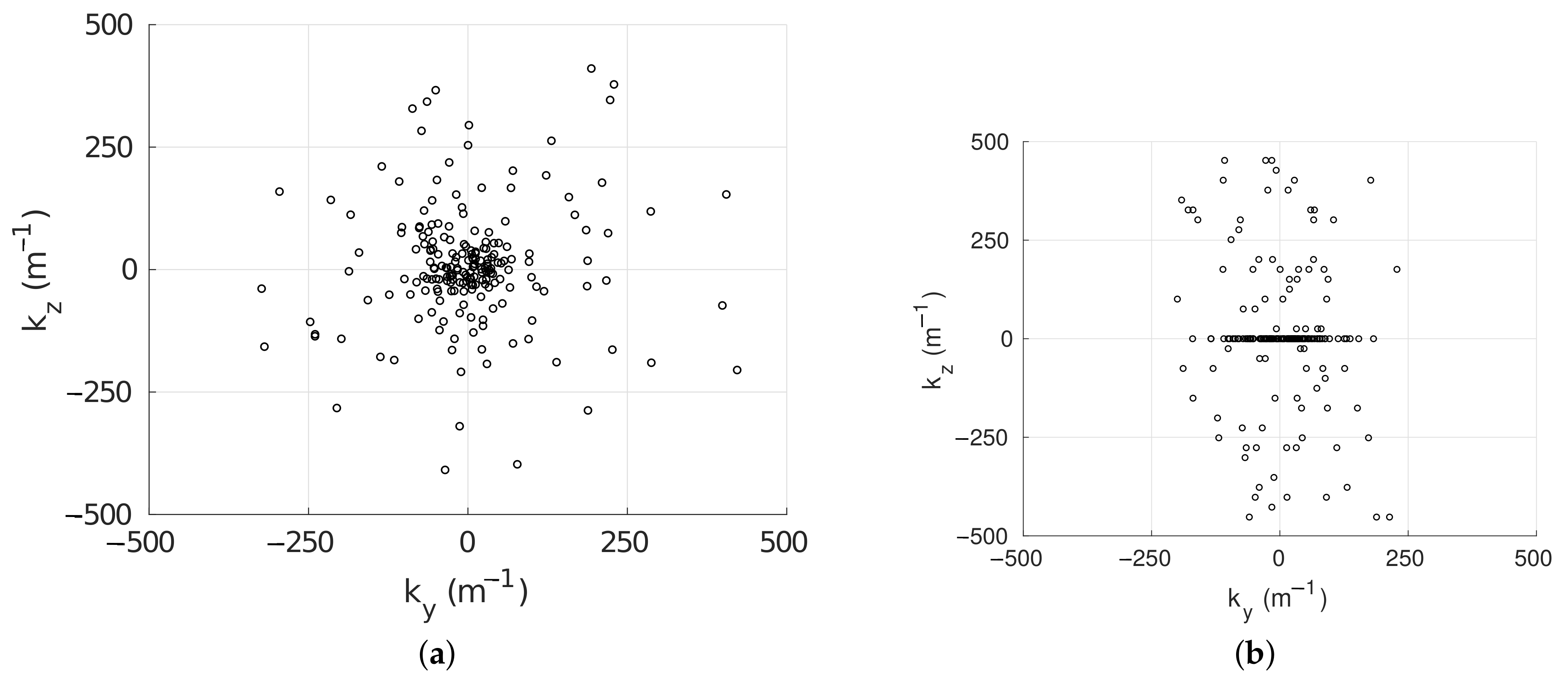
2.2.2. Random Fourier Modes Method Tailored to Periodic Boundary Conditions

In this section, the RFM method is adapted to take into account spanwise periodicity boundary conditions for airfoil simulations. This extension will be called RFM-P in the following, for making a distinction from the RFM method. As the wavenumber components are randomly chosen to respect isotropy in the classical RFM method, spurious noise can be generated when using periodic boundary conditions, as it will be seen in Section 3.2.1. Indeed, a discontinuity of the turbulent velocity is present between the two opposite periodic boundaries. To enforce periodicity, the inflow turbulence is modified by the solver, leading to significant spurious pressure, vorticity and entropy fluctuations. To correct this issue, the spanwise component of the wavenumbers is first chosen in the RFM-P extension as a multiple of the smallest positive wavenumber component respecting the periodicity. Thus, no modification of the inflow turbulence is needed, meaning that the spurious fluctuations disappear. If z denotes the periodic direction, then the only possible values for the z-component of the wavenumbers are

$$k_{nz}=\pm \frac{2\pi n}{L_z},n=1,2,\dots ,N_z,$$

(5)

where $L_z$ is the computation domain length in the z direction and $N_z$ is the number of admissible positive wavenumber components along z. It is defined as

$$N_z=E\left(\frac{k_z^{\mathrm{Max}}}{2\pi /L_z}\right),$$

(6)

where $E\left(•\right)$ is the integer part and $k_z^{\mathrm{Max}}$ is the maximum wavenumber that the mesh can accept, based on the smallest mesh size and on the numerical scheme employed. For example, when using the optimized finite-difference 11-point scheme of Bogey and Bailly [33], this wavenumber must be set to $k_z^{\mathrm{Max}}=\frac{2\pi }{4.6{\mathsf{\Delta }}_z}$ to accurately resolve every injected wave, where ${\mathsf{\Delta }}_z$ is the mesh size in the z-direction. The same notation is adopted for the maximum wavenumbers $k_x^{\mathrm{Max}}$ and $k_y^{\mathrm{Max}}$ along x and y. Then, the RFM-P algorithm computes a set of N targeted wavenumber amplitudes $k_n^{\mathrm{Search}}$ with a logarithmic distribution following Equation (A3). In the second step, randomly chosen wavenumber components $k_{nx}$ and $k_{ny}$ are combined with the admissible values of $k_{nz}$ given by Equation (5) to retrieve the targeted modes. The flow chart for the RFM-P approach is described in Figure 2. Note that the index p is used in this figure, such that the search base corresponding to the wanted wavenumber is written as $k_p^{\mathrm{Search}}$. The pseudo-random wavenumbers are generated using the intrinsic function RANDOM_NUMBER of Fortran Intel compilers. The seed is initialized using the system clock.

The first step of the algorithm consists in generating a maximum number of modes with a non-zero z-component $N_{k_z\ne 0}$, using the values computed by Equation (5). Most of the time, it is impossible to obtain $N_{k_z\ne 0}=N$. Thus, in the second step, a certain number of modes $N_{k_z=0}$ with $k_{nz}$ equal to zero are generated to reach N modes. Eventually, there will be $N_{k_z\ne 0}$ three-dimensional modes and $N_{k_z=0}$ two-dimensional modes. Furthermore, to ensure a maximum of three-dimensional modes, at least one mode must be found for each possible non-zero z-component from Equation (5) or the algorithm will stop. Several iterations (Iteration in Figure 2) can be needed, but only one is usually sufficient so that $N_{\mathrm{iterMax}}$ in Figure 2 can be set to ten. Note also that it is not possible to impose a strict number of modes using the RFM-P extension. Indeed, it becomes difficult to obtain the low-wavenumber amplitudes when the z-component is enforced because it means that the two other wavenumber components must be very small. Thus, an effective number of modes $N_{\mathrm{Eff}}$ exists. To be sure that $N_{\mathrm{Eff}}$ is close enough to N, several iterations (denoted 2DIterationMax in Figure 2) are needed when adding two-dimensional modes. This number of iterations depends on N and on the mesh size. Typically, for the present simulations and $N=200$ modes, 2DIterationMax = 500 is sufficient to obtain $\mid \frac{N_{\mathrm{Eff}}-N}{N}\mid \le 1\%$.

While the RFM method uses random ${\theta }_n$ and ${\varphi }_n$ values for computing the wavenumber components, RFM-P starts from the components to compute the angles in a second step using

$${\theta }_n=arccos\left(\frac{k_{nz}}{k_n}\right)\mathrm{and},$$

(7)

$${\varphi }_n=\left\{\begin{array}{cc}arccos\left(\frac{k_{nx}}{\sqrt{k_{nx}^2+k_{ny}^2}}\right),\hfill & \mathrm{if}{k}_{ny}\ge 0\hfill \\ 2\pi -arccos\left(\frac{k_{nx}}{\sqrt{k_{nx}^2+k_{ny}^2}}\right),\hfill & \mathrm{otherwise}.\hfill \end{array}\right.$$

(8)

The other quantities such as ${\alpha }_n$, $\underline{{\sigma }_n}$, ${\psi }_n$ and ${\tilde{u}}_n$ are computed the same way as in the RFM method described in Appendix A, and the final turbulent fluctuations are calculated using Equation (3). Contrary to the RFM method that is built to respect isotropy, it is clear that the RFM-P approach breaks this isotropy condition by selecting a discrete set of wavenumber values in the periodic direction. This lack of isotropy is illustrated in Figure 3 where the wavenumber distribution is represented for both RFM and RFM-P approaches using a domain length in the periodic direction $L_z=0.25$ m, a search base of $N=200$ modes distributed between 25 and 500 m⁻¹ and $k_x^{\mathrm{Max}}=k_y^{\mathrm{Max}}=k_z^{\mathrm{Max}}=466$ m⁻¹. The number of modes $N_{\mathrm{Eff}}=198$ is obtained, with $N_{k_z=0}=114$ and $N_{k_z\ne 0}=86$. While the RFM method distributes the modes randomly, the RFM-P extension concentrates the modes along the axis $k_x=k_y=0$. It can also be noticed that many two-dimensional structures ($k_z=0$) are obtained. This constraint is, however, thought to be a good approximation when taking a small slice of an airfoil, since most of the structures along z will be aerodynamically seen as two-dimensional structures. One can notice that even with the RFM method, the largest structures will be two-dimensional due to the small span length (2${\mathsf{\Lambda }}_f$), meaning that the isotropy is also broken. When computing leading edge noise in the acoustic far-field, Clair et al. [19] and Atassi [29] explained that only the modes following the relation $k_{nz}\le \frac{k_{nx}M}{\sqrt{1-M^2}}$ will be cut on for an observer in the mid-span plane if the span is at least three times greater than the chord. The mean flow Mach number is denoted $M=U_x/c$, where c is the speed of sound and $U_x$ is the mean flow velocity along x. At a low Mach number, this means that only the modes with a low-wavenumber component in the periodic direction will play a role in the leading edge noise. Thus, taking only two-dimensional structures as Clair et al. [19] did could be a good approximation. However, when M increases, more and more modes will be cut on, meaning that it can be necessary to inject three-dimensional structures to correctly compute the leading edge noise in the mid-span plane, as conducted in the RFM-P approach.

3. Simulations of Spatially Decaying Homogeneous Isotropic Turbulence

In this section, the RFM-P extension is compared to the RFM method, using a case of spatially decaying homogeneous isotropic turbulence (HIT). First, the numerical configurations and the different simulations are described, along with the processing methods. In the second step, the results of both approaches are compared. The aim is to study the turbulence properties between the inlet plane and the close proximity of the airfoil leading edge. Therefore, only the domain between the inlet and the airfoil leading edge is considered in the following. Two meshing configurations are studied. The first one, called Single Grid, serves as a reference since it is a simple box with a constant mesh size. The second configuration, called Multi Grids, is a modified version of Single Grid in order to reduce the computational cost. Details are given in Section 3.1.1. A comparison of the turbulence properties between both configurations and both synthetic turbulence generation approaches will be performed. Since the turbulence is stochastic, the present results may depend on the particular turbulence realization. Thus, the results of two different realizations are presented for the Single Grid configuration only. Some data and results of this section are available in the Supplementary Materials at the end of the conclusion.

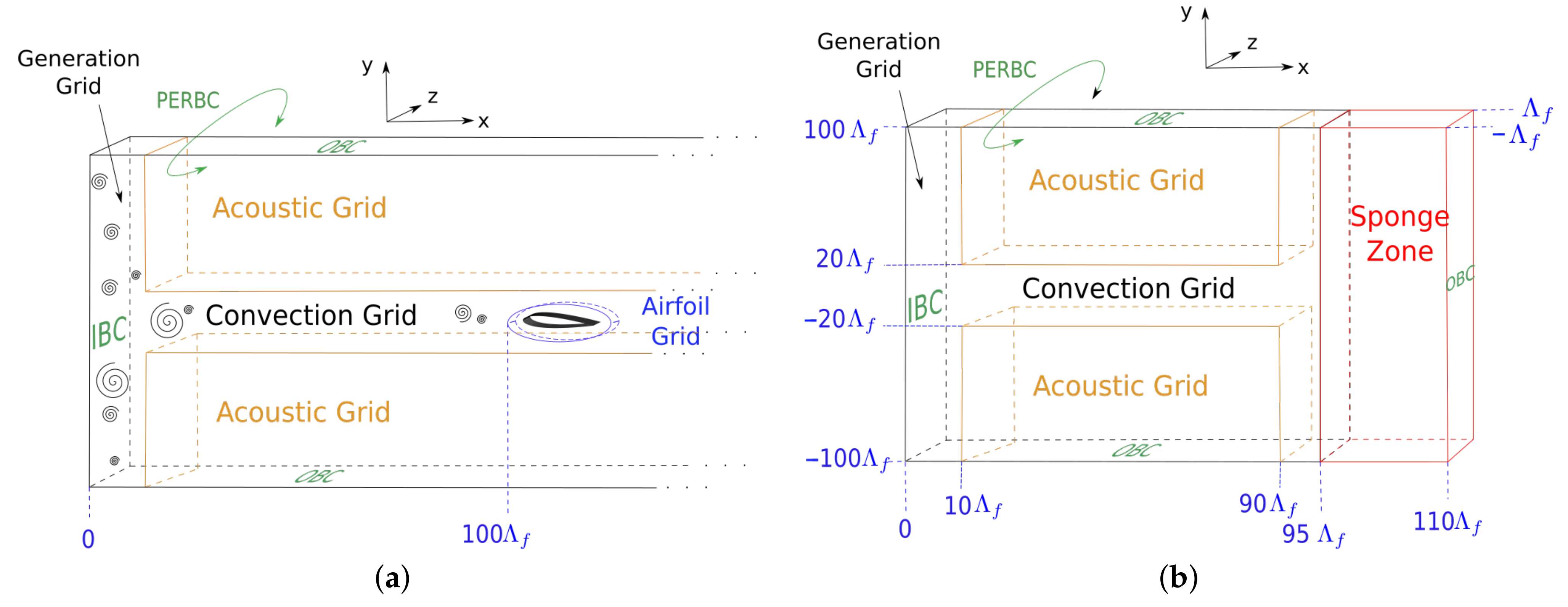
3.1. Studied Configurations and Numerical Setups

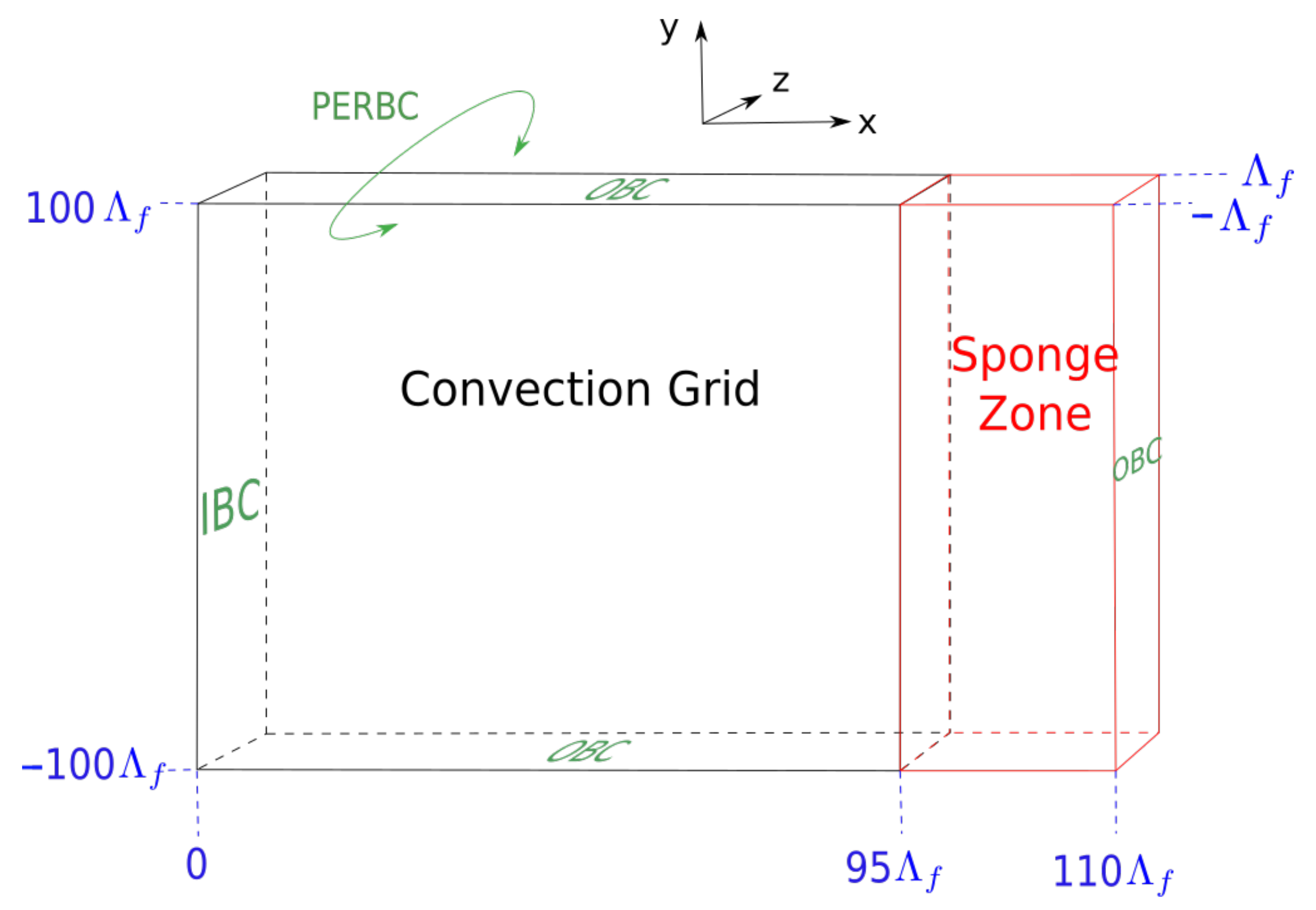
3.1.1. Configurations

The inflow turbulence is based on Comte-Bellot and Corrsin’s [40] results taken at their first measurement plane. They give the longitudinal integral length scale ${\mathsf{\Lambda }}_f$ and the turbulent kinetic energy $k_t$, whose values will be given in Section 3.1.2. These two quantities drive the configuration numerical setups. The Single Grid configuration is shown in Figure 4 and is first composed of a main grid, called the convection grid, with a uniform mesh size $\mathsf{\Delta }$. Then, at the end of the domain, a sponge zone is added to damp turbulent structures before they reach the exit boundary. The boundary conditions, described in Section 2.1, are also presented in this figure: IBC stands for inflow boundary condition, OBC for outflow boundary condition and PERBC for periodic boundary condition. The dimensions of the computational domain are based on similar configurations found in the literature. The domain length along x is set to $L_x=9.5c$, where c is the virtual airfoil chord. Indeed, Eljack [41] or Thomareis and Papadakis [42] showed by some convergence tests on a NACA0012 that this distance, between the inlet and the airfoil leading edge, is sufficient to have convergence on the pressure and friction coefficients, even when an LSB is present. The sponge zone length along x is equal to 1.5c, beginning at 9.5c. Similarly, the $L_y$ computational domain length, in the chord-normal direction, is set to 20c. Finally, the airfoil span is set to $L_z=0.2c$ to limit the computational cost. The chord is set to $c=10{\mathsf{\Lambda }}_f$, as it can been found in the experiments of Wang et al. [3] or Moreau et al. [43]. The data transfer between the convection grid and the sponge zone is ensured by an 8th-order interpolation [30]. The mesh size $\mathsf{\Delta }$ for turbulence convection up to the airfoil is set to $\mathsf{\Delta }={\lambda }_g/1.1$ to have enough resolved structures, where ${\lambda }_g$ is the transverse Taylor micro-scale of the injected turbulence.

Then, to decrease the computational cost, the Multi Grids configuration is proposed. The motivation behind this configuration is to reduce the size of the convection grid along the y axis, as shown in Figure 5a where an airfoil is drawn only for clarity purposes. The remaining computational domain is composed of a generation grid at the inlet with a mesh size equal to $\mathsf{\Delta }$ and of two acoustic grids with a mesh size equal to $2\mathsf{\Delta }$, since no turbulence is needed in these areas. The acoustic grids begin at 10${\mathsf{\Lambda }}_f$ downstream of the inlet plane to avoid an interaction with the generation grid. The turbulence is convected from the inlet plane towards the airfoil through the convection grid, while the smallest scales are dissipated when passing through the acoustic grids. As no airfoil is needed in the present study, Figure 5b displays the geometry considered in the present work. The configuration is basically the same but a sponge zone is added at the computational domain exit as in the Single Grid configuration. Boundary conditions and dimensions for acoustic and convection grids are given in the figure. The convection grid has a height of 40${\mathsf{\Lambda }}_f$. Global dimensions are the same as those for the Single Grid configuration. In the acoustic grids, the small structures whose wavelengths respect $\lambda <4.6\mathsf{\Delta }$ are numerically damped by the filter during their convection by the mean flow. The advantage of this second configuration is that it halves the number of calculation points. Details such as the total number of points for both configurations are given in

Table 1. Geometrical and mesh data for both Single Grid and Multi Grids configurations. ${\mathsf{\Lambda }}_f$ stands for the longitudinal integral length scale and ${\lambda }_g$ for the transverse Taylor micro-scale of the turbulence.

Configuration	$\frac{{\mathit{L}}_{\mathit{x}}}{{\mathsf{\Lambda }}_{\mathit{f}}}$, $\frac{{\mathit{L}}_{\mathit{y}}}{{\mathsf{\Lambda }}_{\mathit{f}}}$, $\frac{{\mathit{L}}_{\mathit{z}}}{{\mathsf{\Lambda }}_{\mathit{f}}}$	Mesh Size in Convection Grid	Mesh Size in Acoustic Grids	Number of Mesh Points	Number of Interpolation Points
Single Grid	95, 200, 2	${\lambda }_g/1.1$	/	6.79 × 106	1.07 × 105
Multi Grids	95, 200, 2	${\lambda }_g/1.1$	$2{\lambda }_g/1.1$	3.34 × 106	2.08 × 105

.

3.1.2. Simulation Parameters

For each configuration, three simulations are carried out. The first simulation is conducted with the RFM method described in Section 2.2.1, the second simulation with the RFM-P extension described in Section 2.2.2 and the third one with the RFM-P approach, but only with two-dimensional structures, meaning that $k_z=0$ for every mode. The simulations are respectively named RFM, RFM-P3D and RFM-P2D. The physical turbulence parameters are those measured by Comte-Bellot and Corrsin [40] in their wind tunnel first plane, that are $k_t=0.0739$ m²·s⁻², ${\mathsf{\Lambda }}_f=0.024$ m and ${\lambda }_g=0.0048$ m. This gives a Reynolds number of $R{e}_{{\lambda }_g}=\frac{{\lambda }_g\sqrt{2/3k_t}}{\nu }=72$, where $\nu$ is the kinematic viscosity. This low Reynolds number could be problematic for subgrid models, particularly for the classical models which assume a large separation between small and large turbulent scales. The numerical filtering used in the present work has the advantage of overcoming this limitation, meaning that the mesh size only determines the spectral range that is resolved [32].

The modified von Kármán spectrum is discretized with $N=$ 200 modes between 20 and 500 m⁻¹ since the energy is concentrated in this wavenumber range. In addition, for the RFM-P extension, the maximum wavenumber in each direction is chosen according to the accurate limit of resolution of the 4th-order 11-point scheme such that $k_x^{\mathrm{Max}}=k_y^{\mathrm{Max}}=k_z^{\mathrm{Max}}=335$ m⁻¹ ≃ $\frac{2\pi }{4.6\mathsf{\Delta }}=313$ m⁻¹. The accurate limit is a little bit exceeded so that more modes can be introduced, but it is important to note that all the modes are still resolved by the scheme and the mesh.

The Mach number is set to $M=U_x/c=0.1$, giving a turbulent intensity of $I_t=\frac{\sqrt{2/3k_t}}{U_x}=0.65\%$. The Mach number is greater than the one of Comte-Bellot and Corrsin’s experiments because of the high computational cost and bad conditioning of Code_Safari at low Mach numbers. The CFL number is equal to 0.95 to ensure stability and to reduce diffusion or dispersion errors brought by the chosen schemes. Simulations are carried out on 12$t_{L_x}^{*}=\frac{N_{\mathrm{ite}}{\mathsf{\Delta }}_t{U}_x}{L_x}$, where $t_{L_x}^{*}$ is the normalized convection time based on $L_x$ and $U_x$, ${\mathsf{\Delta }}_t$ is the time step and $N_{\mathrm{ite}}=7.14\times {10}^4$ is the number of computation iterations. The numerical filtering strength is set to ${\sigma }_{\nu }=0.2$, as in Bogey and Bailly [44]. As already seen in Section 2.2.2, an effective number of modes $N_{\mathrm{Eff}}$ is obtained, whose values are given in

Table 2. Desired mode number N, effective mode number $N_{\mathrm{Eff}}$ and three-dimensional structure number $N_{3D}$ for the simulations.

Simulation	N	${\mathit{N}}_{\mathbf{Eff}}$	${\mathit{N}}_{3\mathit{D}}$
RFM_Single_Grid	200	200	200
RFM-P3D_Single_Grid	200	198	68
RFM-P2D_Single_Grid	200	196	0
RFM_Multi_Grids	200	200	200
RFM-P3D_Multi_Grids	200	199	62
RFM-P2D_Multi_Grids	200	196	0
RFM_Single_Grid_Realization2	200	200	200
RFM-P3D_Single_Grid_Realization2	200	200	67
RFM-P2D_Single_Grid_Realization2	200	196	0

, as well as the number of three-dimensional structures $N_{3D}$ in the RFM-P3D simulations. The effective number of modes is close to the target value, with a maximum relative error of 2%.

Finally, the three simulations of the Single Grid configuration are conducted for another turbulence realization to study the influence of different mode draws, the second realization being independent from the first one. The corresponding simulation names end with _Realization2 in Table 2.

3.1.3. Probes and Processing Method

In this section, the sets of probes used to compute the resolved turbulent kinetic energy and the one-dimensional spectra are described. These quantities are calculated using data on the last 2$t_{L_x}^{*}$. The resolved turbulent kinetic energy $k_t^r$ along x is studied with a line of probes placed at $y=z=0$ and with a 3$\mathsf{\Delta }$ space between two successive probes. The longitudinal spectral power density $E_{vv}\left(k_y\right)$ of the y-velocity v is computed on $x=0$ and $x=90{\mathsf{\Lambda }}_f$. On each x position at $z=0$, 106 probes are placed between $y=-10{\mathsf{\Lambda }}_f$ and $y=10{\mathsf{\Lambda }}_f$ with a $\mathsf{\Delta }$ space between each successive probe. The minimum and maximum y positions are chosen so that enough probes can be placed without being in the interpolation areas between convection and acoustic grids. The periodogram method is used to compute the spectra using all 106 points on each x position. Thus, these spectra have a spectral resolution of 13 m⁻¹ and a sampling wavenumber of 1400 m⁻¹. They are computed at each iteration of the last 2$t_{L_x}^{*}$ and averaged on this time window.

3.1.4. Computation Platform and MPI Decomposition

Simulations are carried out on Occigen, a supercomputer belonging to the CINES (French National Computing Center for Higher Education). Only Haswell [email protected] processors are used with an Infiniband FDR 56 Gbit/s communication bus. The 2.0.1 OpenMPI library for Intel compilers is employed. The distribution of cores in simulations is conducted so that each core has roughly the same number of calculation points in each direction, both in Single Grid and Multi Grids configurations, except in the z direction where there are not enough calculation points to cut the domain into several processes. For this purpose, the Single Grid simulations are run with 180 cores spread on 8 nodes of 24 cores, while the Multi Grids simulations are carried out on 140 cores spread on 6 nodes of 24 cores. Thus, it is important to notice that the number of cores and their distribution on the grids are not the same between Single Grid and Multi Grids configurations for core layout optimization. For each configuration, the number of points per core in the three directions is given in

Table 3. Number of points per core for each configuration in every direction (see Figure 4 and Figure 5).

	Single Grid			Multi Grids
	x	y	z	x	y	z
Convection Grid	60	60	11	48	43	11
Sponge Zone	40	60	11	40	53	11
Acoustic Grids	/	/	/	48	53	6
Generation Grid	/	/	/	81	53	11

. The numbers of interpolation points, due to the interface between acoustic and convection grids and the sponge zone, are given in Table 1 for both Single Grid and Multi Grids configurations. As the calculation point number decreases with the Multi Grids configuration, the number of interpolation points increases, which must be taken into account when estimating the computational cost.

3.2. Comparison of the RFM and RFM-P Approaches for Both Configurations

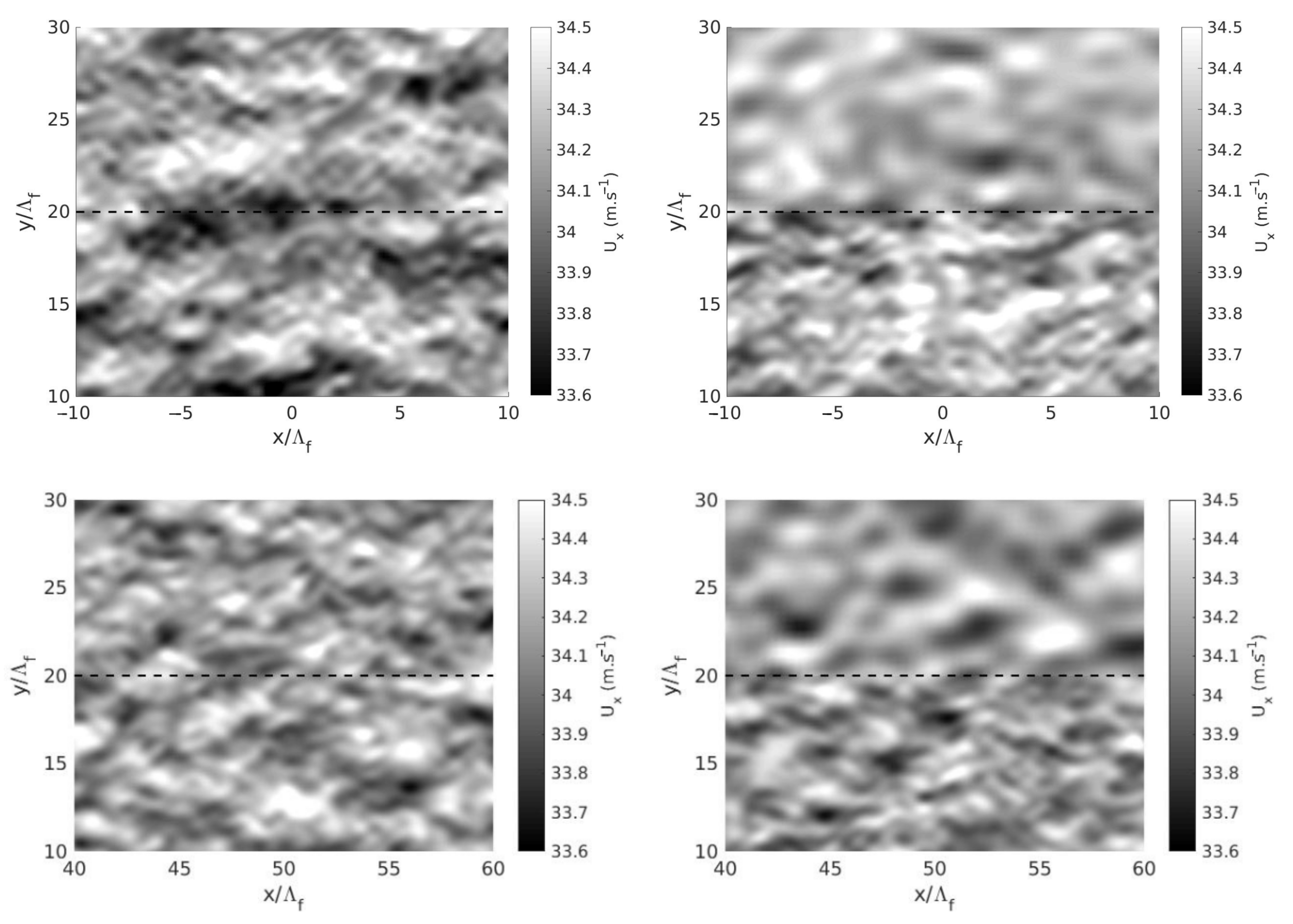
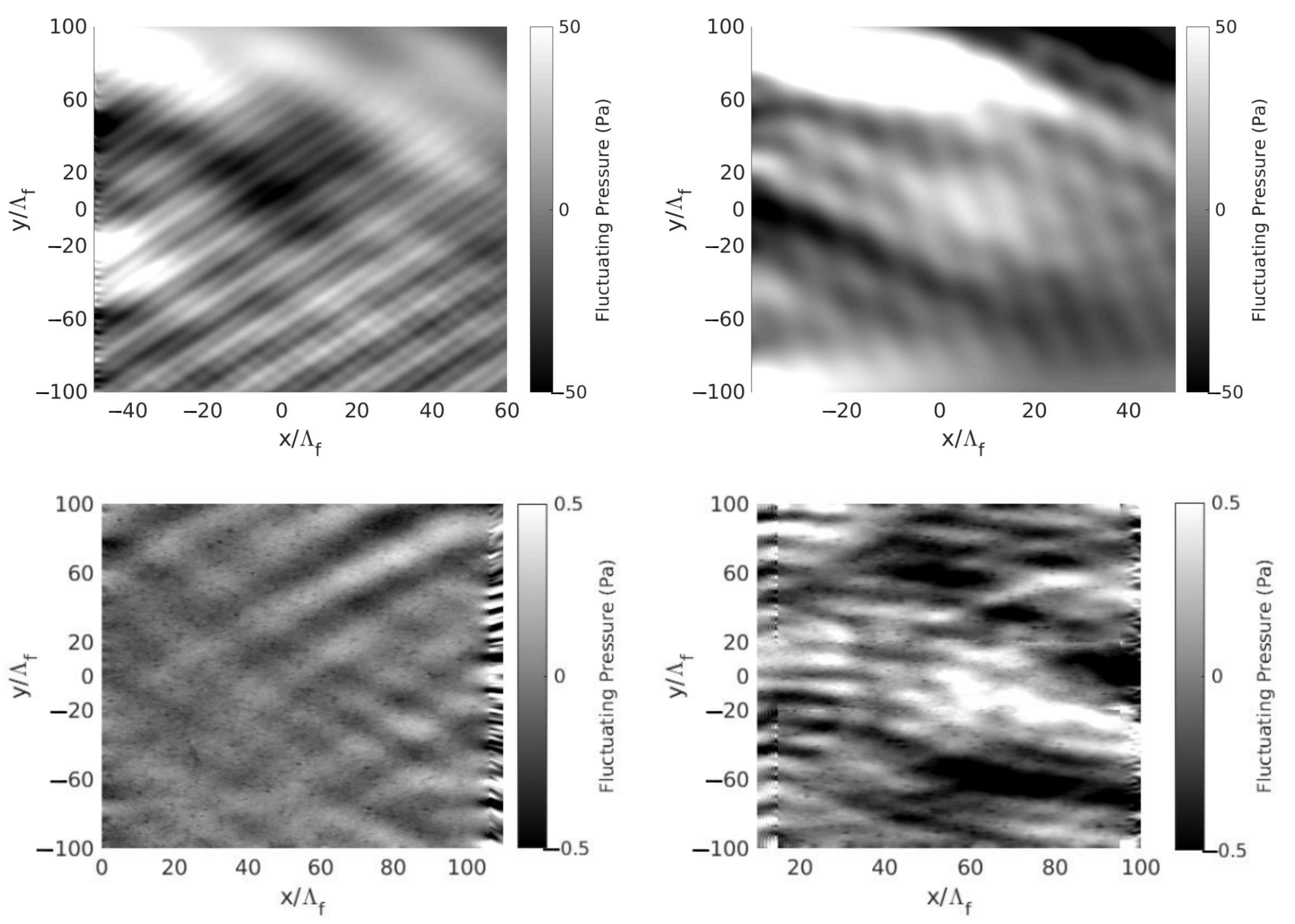
3.2.1. Instantaneous Velocity and Pressure Fields

Instantaneous x-velocity at $z=0$ is shown at the last iteration in Figure 6 for both Single Grid and Multi Grids configurations and for both RFM and RFM-P3D simulations. The velocity fields are zoomed in on the frame [40${\mathsf{\Lambda }}_f$,60${\mathsf{\Lambda }}_f$] × [10${\mathsf{\Lambda }}_f$,30${\mathsf{\Lambda }}_f$]. In the Single Grid configuration, small and large scales can be observed in all of the domain, while for the Multi Grids configuration, small scales can only be seen in the convection grid in both figures. No significant differences are visible between RFM and RFM-P3D simulations, considering both configurations.

Similarly, the corresponding fluctuating pressure fields at $z=0$ are shown in Figure 7. There is a high decrease in the spurious noise between RFM and RFM-P3D simulations. It is worth mentioning that the pressure is scaled between −50 and 50 Pa for the RFM simulations, while it is scaled between −0.5 and 0.5 Pa for the RFM-P3D simulations. This represents the main result of the paper, in that the RFM-P extension does not significantly affect the velocity field, while it strongly reduces the spurious noise. When considering only the RFM-P3D simulations in Figure 7, it can be seen that the pressure fields have higher levels in the Multi Grids configuration than in the Single Grid one. This issue can be attributed to the overset method where interpolations take place. As explained by Sharan et al. [45], numerical dispersive waves can be reflected between the different grids of the mesh. These waves can grow with time and pollute the computational domain. For the Single Grid configuration, noise is mainly radiated from the sponge zone. This will not be a problem for airfoil computations, since the sponge zone will be far behind the airfoil and will be extended to a longer distance to make it more efficient.

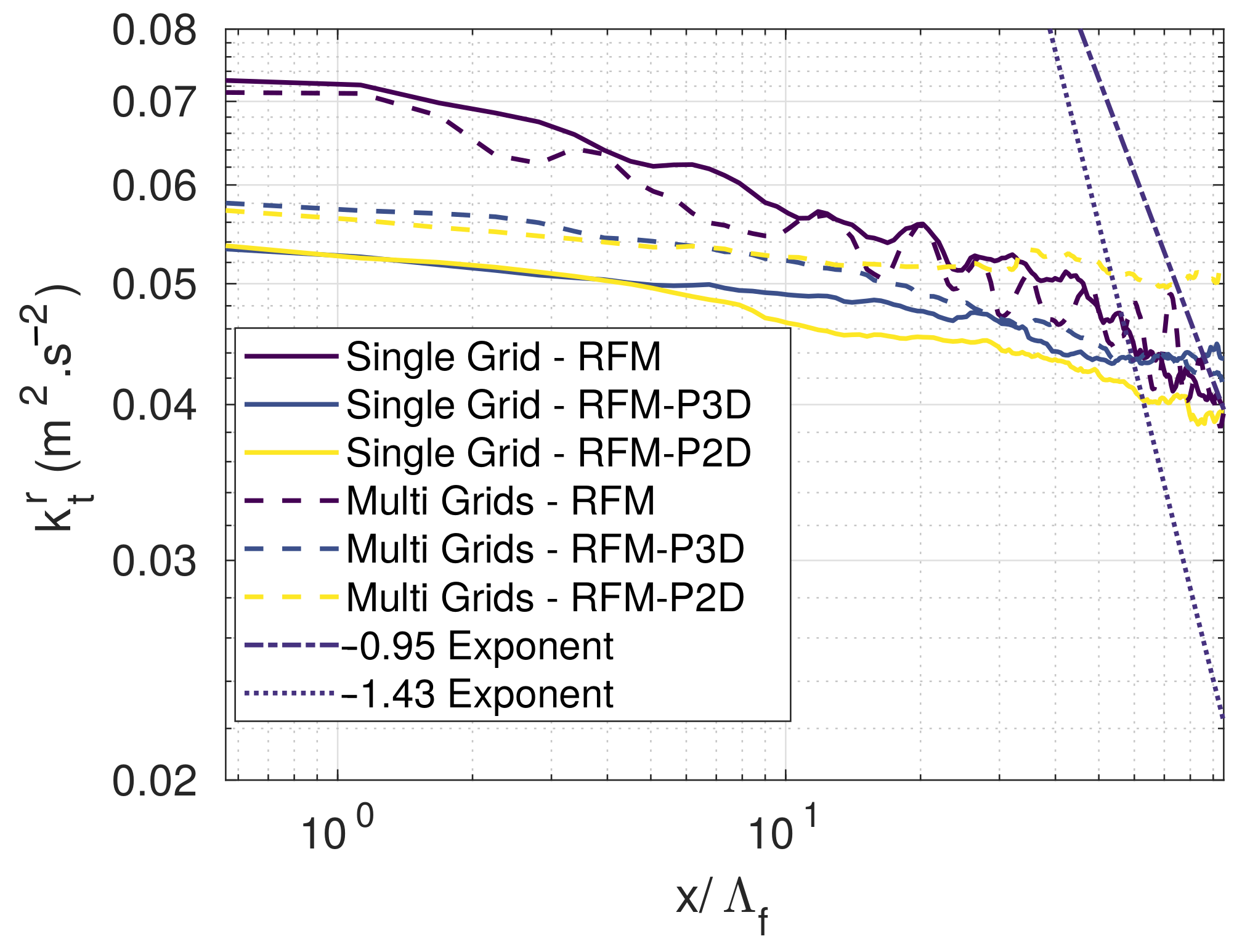
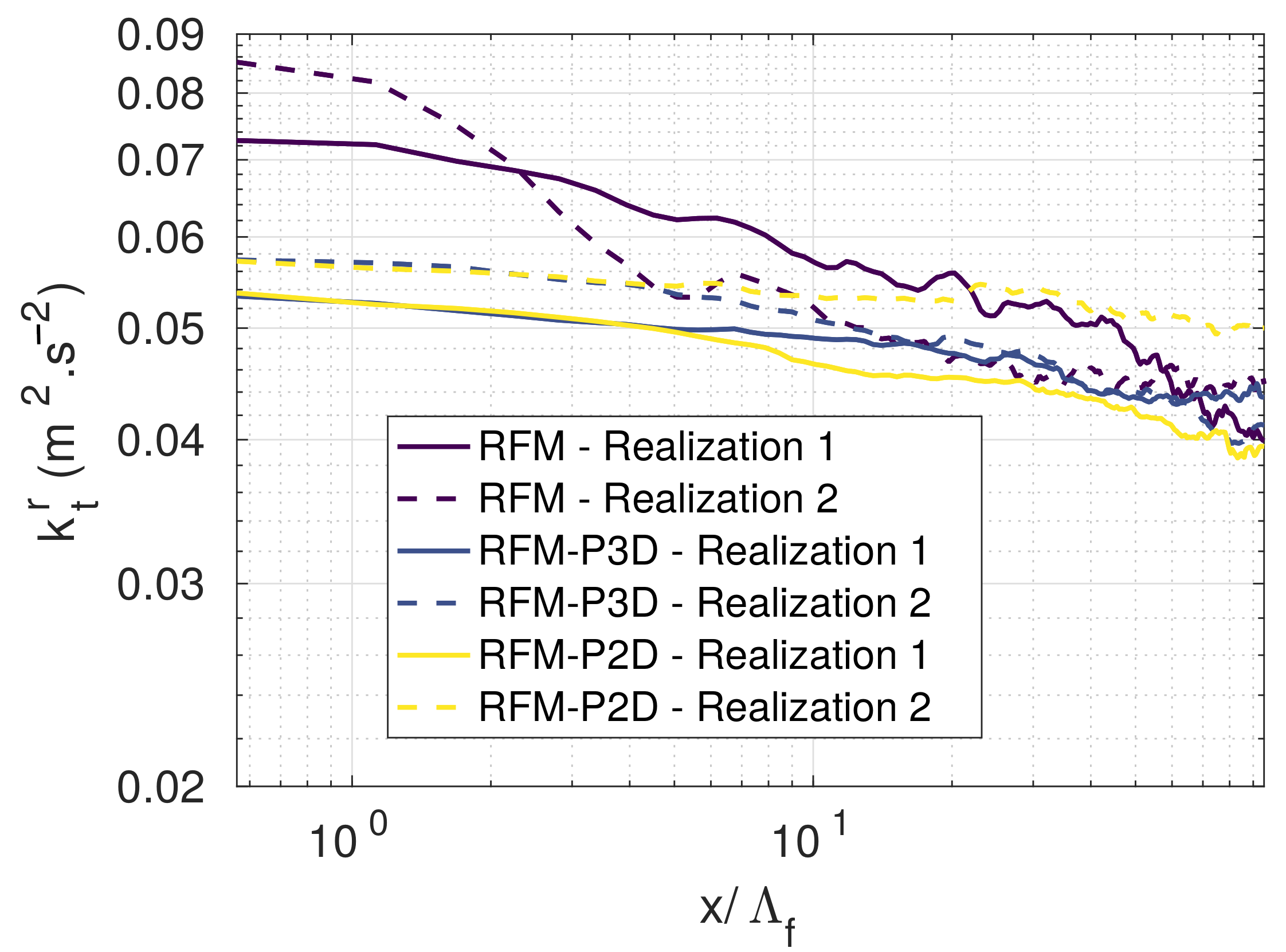
3.2.2. Turbulent Kinetic Energy Evolution

Figure 8 shows the decay of the resolved turbulent kinetic energy $k_t^r$ using probes described in Section 3.1.3. In LES, only a part of the spectrum is calculated; thus, the resolved kinetic energy $k_t^r$ is smaller than the total turbulent kinetic energy $k_t$. In the present work, $k_t^r$ is estimated as 0.055 m²·s⁻² at the inlet, with $k_t=$ 0.0739 m²·s⁻². From Figure 8, it can be seen that RFM-P simulations are close to this value for both configurations, but the RFM simulations overestimate it. As the RFM method is not suitable for periodic boundary conditions, the solver must strongly adapt velocity and pressure fields to enforce the periodicity which causes the generation of high-amplitude undesired waves. It is important to note that the velocity fluctuations are not directly superimposed to the mean flow but computed through Equation (2). Thus, they can be modified right at the inlet if they do not respect the periodicity condition. This explain why the resolved turbulent kinetic energy takes different values on x = 0 depending on the simulation. Additionally, this issue is present because the span is very small (only 2${\mathsf{\Lambda }}_f$, 11 computational points), that means that all the points of the domain are affected by the periodicity condition, contrary to the study [46], where the span was 5${\mathsf{\Lambda }}_f$ and the turbulent kinetic energy of every simulation started from the same value. However, the high-amplitude spurious noise problem was present even in this configuration.

The extreme values of the empirical decay exponent for grid-generated turbulence [47] are also plotted in Figure 8, showing that the spatial decay is really small in the simulations. For RFM-P simulations, 25% of the initial energy is lost when reaching the airfoil leading edge. This spatial loss should increase if the mean velocity decreases, giving more time for dissipation. Indeed, considering $\frac{d{k}_t}{dt}=-ϵ$ [48], where $ϵ$ is the turbulent kinetic energy dissipation rate, and assuming a frozen turbulence, the evolution of $k_t$ with respect to x is $\frac{d{k}_t}{dx}=-\frac{ϵ}{U_x}$, $ϵ$ being independent from $U_x$.

If the turbulence temporal decay does not depend on the Mach number, its spatial decay does, as seen above. Here, $M=0.1$ is sufficiently low to be able to capture some changes in the turbulence statistics during its convection along the domain length $L_x$. Indeed, the convection time at a distance of $L_x=$ 95${\mathsf{\Lambda }}_f$ can be expressed as

$${\tau }_{L_x}=6.7\times {10}^{-2}\mathrm{s}=11.75{\tau }_{\eta }={\tau }_{{\mathsf{\Lambda }}_f}/1.61,$$

(9)

where ${\tau }_{\eta }=\sqrt{\frac{\nu }{ϵ}}$ is the Kolmogorov time scale and ${\tau }_{{\mathsf{\Lambda }}_f}=\frac{{\mathsf{\Lambda }}_f}{\sqrt{2/3k_t}}$ is the decaying time for the largest scales. Thus, only the small scales have the time to evolve in this particular situation, meaning that the small spatial decay observed could only be a consequence of the relatively high Mach number of this particular situation in comparison with the Mach number of Comte-Bellot and Corrsin’s experiments [40]. The ratio between the numerical and experimental turbulent kinetic energy spatial decays can be expressed as $\frac{{\left.\frac{d{k}_t}{dx}\right|}_{\mathrm{Simu}.}}{{\left.\frac{d{k}_t}{dx}\right|}_{\mathrm{Expe}.}}=\frac{M^{\mathrm{Expe}.}}{M^{\mathrm{Simu}.}}=0.37$. Additionally, the same small energy decay was already observed in a previous study [46] using the same numerical tools but with a larger domain length $L_x=250{\mathsf{\Lambda }}_f$. As a consequence, the convection time was comparable to the large-scale decaying time. Thus, even when the large scales have the time to evolve during their convection, most of the dissipation is due to the small scales, meaning that the turbulent kinetic energy should remain nearly the same at a sufficiently long distance to reach the airfoil leading edge.

The fact that the numerical decay is not in agreement with the empirical one comes from the synthetic turbulence generation method. Indeed, the third-order moment is not reproduced and this moment is responsible for the energy transfer from the large scales to the smallest, as explained by Dhamankar et al. [11] in their review. However, for airfoil simulations, this disagreement can be beneficial since the turbulent kinetic energy at the leading edge can be the same as or very close to the energy set at the inlet. Finally, Figure 8 shows that the energy using the Multi Grids configuration increases slightly compared to the one of the Single Grid configuration for RFM-P simulations. This increase is of 7% only. To explain it, Figure 9 compares the turbulent kinetic energy decay obtained for two different turbulence realizations using the Single Grid configuration. One can notice that the results between the two realizations are different and that the increase in the kinetic energy in the second realization is similar to the one obtained in Figure 8 with the Multi Grids configuration. The overestimation with the RFM method is still present compared to the other simulations. Thus, the difference in the kinetic energy between the Multi Grids and Single Grid configurations in Figure 8 is not necessarily the consequence of the different configurations but of the different realizations. The increase in the energy in Figure 8 for the Multi Grids-RFM-P2D simulation after 20${\mathsf{\Lambda }}_f$ is also due to the realization variability since the same behavior is visible in Figure 9 for Realization 2 in the Single Grid-RFM-P2D simulation. More realizations would be desirable to compute an uncertainty error in the method, but that would also be very computationally expensive.

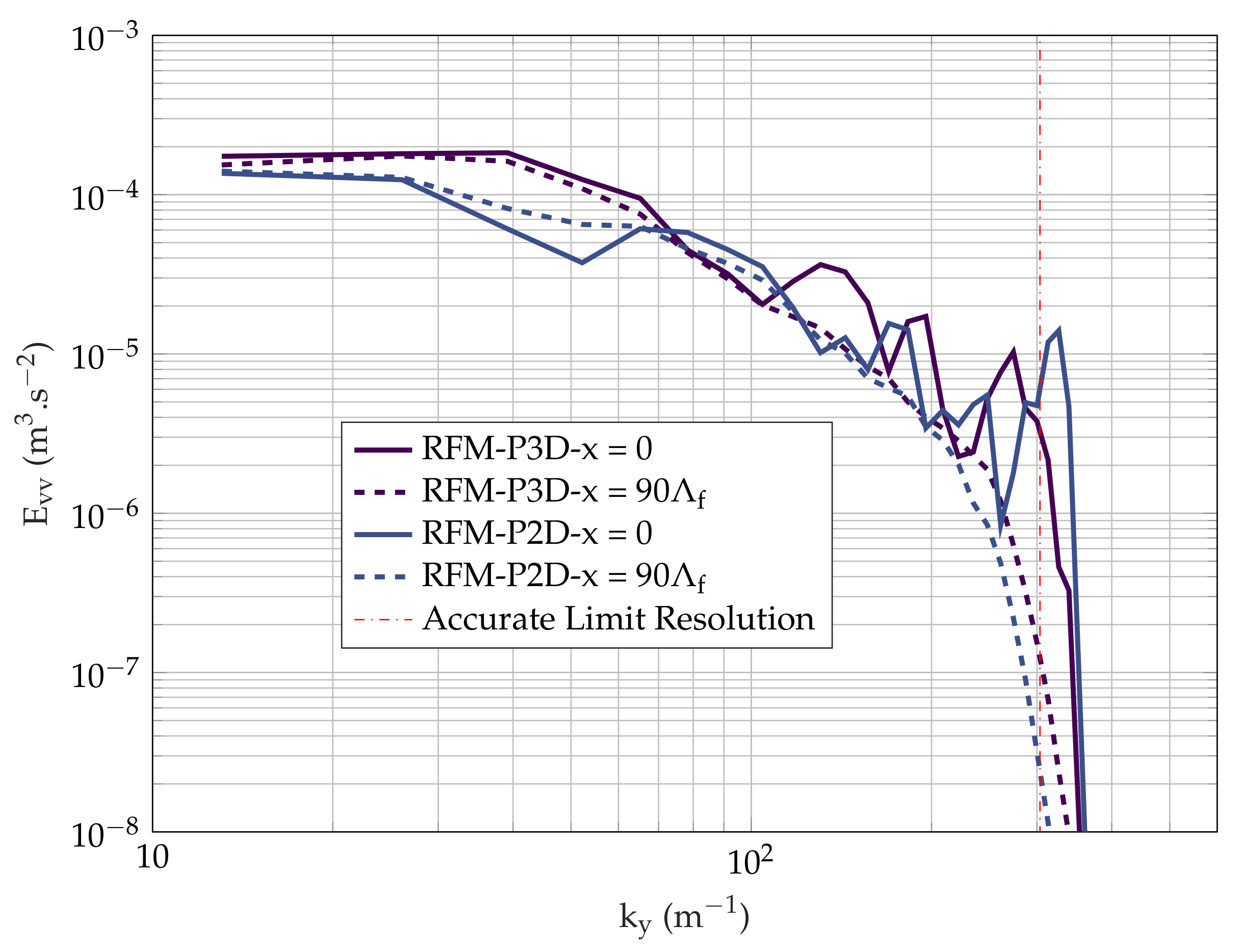
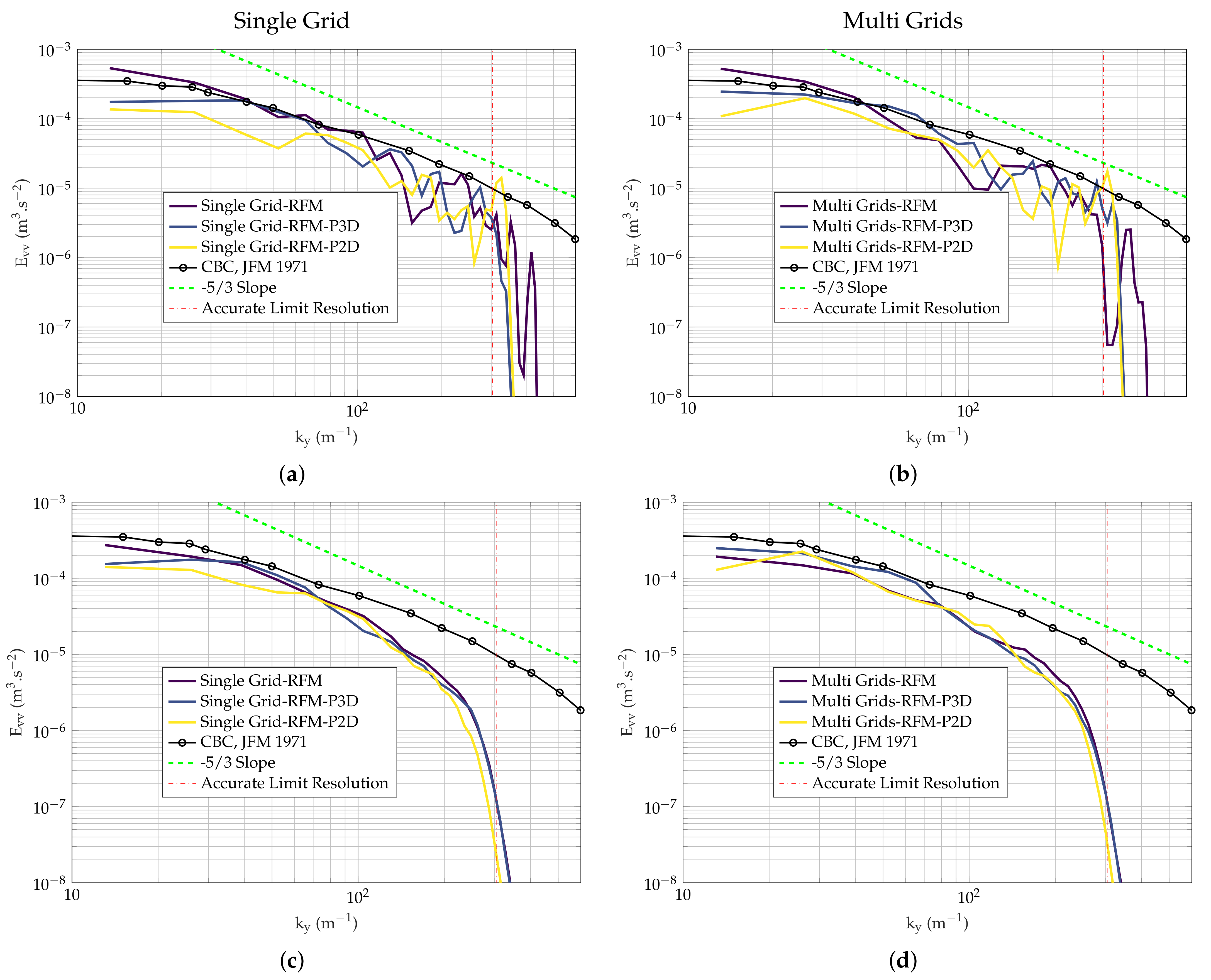
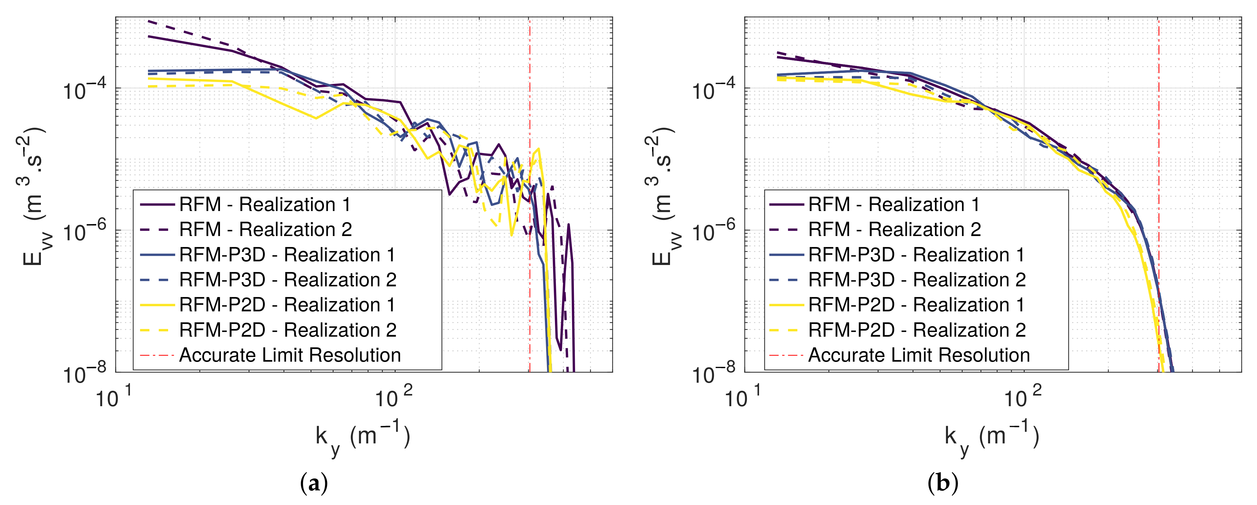
3.2.3. One-Dimensional Spectra

One-dimensional spectra $E_{vv}$ along the y direction are obtained using probes described in Section 3.1.3. The top plots of Figure 10 show these spectra for the Single Grid and Multi Grids simulations at the box inlet, $x=0$, while the bottom plots show the same spectra at $x=90{\mathsf{\Lambda }}_f$. The resolution limit plotted as a vertical line corresponds to the smallest wavenumber that can be accurately calculated by the numerical scheme with the chosen mesh size. First, by comparing Figure 10a and Figure 10b, similar results are obtained between configurations Single Grid and Multi Grids at the inlet. The simulations are also compared to the measurements of Comte-Bellot and Corrsin [40], showing that both methods are capable of reproducing the desired experimental spectrum. However, the RFM method seems to overestimate the energy at the lowest wavenumber which can be explained by the same reason given for the kinetic energy overestimation in Section 3.2.2. The RFM-P extension tends to underestimate the energy at the lowest wavenumber. This could be due to the small domain length $L_z=2{\mathsf{\Lambda }}_f$, that may not be sufficient to introduce the largest scales. Indeed, using the same turbulence parameters, it was observed in [46] that the energy was correctly computed at the lowest wavenumber when the domain length along z was more than twice the present one.

A different behavior is observed at intermediate wavenumbers (30 m⁻¹ ≤ $k_y$ ≤ 60 m⁻¹). On the one hand, the RFM and RFM-P3D approaches are close to each other. On the other hand, the RFM-P2D simulation shows lower energy levels compared to the two other simulations at $x=0$. An explanation for this observation will be proposed later in this section.

Spectra right at the inlet are not the best criteria to assess the relevance of the RFM-P extension. Indeed, peaks in the spectra are present because of the discrete distribution of the energy between modes. It is necessary to look at the spectra near the end of the computational domain since this will be the location of the airfoil leading edge in future simulations. The adaptation distance between the inlet and the outlet allows the energy transfer between modes to be carried out by the Navier–Stokes equations. Spectra in Figure 10c,d are indeed smoother, and the three simulations give similar results. The high-wavenumber energy has been numerically dissipated between $x=0$ and $x=90{\mathsf{\Lambda }}_f$ because of a lack of grid resolution, as the red dashed vertical line shows. Retrieving high-wavenumber energy is only possible by decreasing the mesh size. The RFM-P simulation with two-dimensional structures seems to be, again, less energetic than the other simulations at low wavenumbers, but only for the Single Grid configuration. Note that the Comte-Bellot and Corrsin [40] measurements correspond to the inlet plane ($x=0$) for all plots of Figure 10. It is not possible to compare numerical spectra at $x=90{\mathsf{\Lambda }}_f$ with measurements at the same location because the mean flow velocity is different from the one used in the experiments.

Finally, Figure 11 shows the results between both planes for the Single Grid configuration and only for the RFM-P extension because the RFM method was shown to overestimate the low-wavenumber energy due to the periodicity problem. It can be seen that the energy at low wavenumbers is nearly the same between both positions, while the energy at high wavenumbers is dissipated. Spectra become smoother and non-resolved scales are attenuated, that explains the decay of the turbulent kinetic energy in Figure 8. It means that the large structures are purely convected and that the transfer towards the small scales does not take place, as already explained. Notice that smaller scales could be added to the simulation by reducing the mesh size. Thus, a full range of scales could be obtained, without dissipation between the inlet and the airfoil.

As conducted for the kinetic energy, the results for a second turbulence realization are compared with those of the first realization for the Single Grid configuration in Figure 12. On the first plane, results between realizations seem to be quite similar for low wavenumbers only. The difference visible at high wavenumbers comes from the different distributions of modes between realizations. On the second plane, the difference between the two realizations can hardly be seen, and the RFM-P2D simulation still contains less energy at low wavenumbers. Looking at Figure 10, Figure 11 and Figure 12 for $x=0$, the RFM-P2D simulation is less energetic for $k_y\le 70$ m⁻¹. This is a consequence of the algorithm of Figure 2 used to generate the wavenumbers. Indeed, setting $k_z=0$ allows greater values of $k_y$ to be reached in order to fill all the wavenumbers $k=\sqrt{k_x^2+k_y^2+k_z^2}$ of the desired spectrum. Thus, more energy is injected at higher values of $k_y$ compared to the RFM-P3D simulation where $k_z\ne 0$. In conclusion, regarding spectra, the RFM-P3D simulation gives better results than the RFM one because there is no energy overestimation at the inlet for the lowest wavenumbers.

3.2.4. Computational Cost

In this section, the computational costs of all simulations are presented. Section 3.1.4 should be kept in mind while reading the present results since the distribution and number of cores are not the same between configurations, meaning that the performance’s results are approximate.

Table 4. Computational cost of each simulation.

Simulation	Cost (Core Hours)
RFM_Single_Grid	6150
RFM-P3D_Single_Grid	6150
RFM-P2D_Single_Grid	6300
RFM_Multi_Grids	4700
RFM-P3D_Multi_Grids	4750
RFM-P2D_Multi_Grids	4600

shows the computational cost in core hours for each simulation. The Multi Grids configuration seems to be less expensive which is due to the smaller mesh number in comparison with the Single Grid configuration. A gain of 25% in the computational cost can be achieved, which can be useful for expensive airfoil simulations.

4. Conclusions

To compute airfoil leading edge noise and to trigger boundary layer instabilities using compressible large eddy simulations, synthetic turbulence compatible with periodic boundary conditions is needed. When the classical random Fourier modes method is used to generate synthetic turbulence, spurious noise is present because this method does not respect the periodicity condition in the spanwise direction, since the wavenumber components are randomly chosen. In the present work, an adaptation of the random Fourier modes method for periodic boundary conditions, called the RFM-P extension, was developed and compared with the RFM method in a case of spatially decaying homogeneous isotropic turbulence, using two-dimensional or three-dimensional modes. The RFM-P algorithm computes modes whose wavenumber component in the lateral direction is compatible with the periodic boundary condition. Two geometrical configurations were considered to study the spatial decay of turbulence using both approaches. The first configuration, called Single Grid, is a simple box with a constant mesh size, and the second one, called Multi Grids, reduces the computational cost by up to 25% by decreasing the mesh size where detailed turbulence is not needed. Results show that the RFM-P extension permits a better control of the turbulent kinetic energy compared to the RFM method, while the spectral shape is not disturbed. Furthermore, the decay of the turbulent kinetic energy is small compared to the empirical decay exponents. This decrease is only due to the dissipation of the smallest scales, while larger scales are unchanged and purely convected towards the outlet. The RFM method produces undesired high-amplitude waves generated at the inlet to force the turbulent fluctuations to be periodic. The RFM-P extension, developed in this work, is effective in getting rid of these waves. The drawback of the second configuration is the interpolation using the Chimera method, which causes additional spurious pressure fluctuations at the inlet compared to the constant mesh size configuration. In the future, the RFM-P approach will be tested in airfoil simulations to study the effect of inflow turbulence on the broadband noise emitted by an airfoil at various angles of attack.

Finally, the authors of the present work are aware of the RFM-P extension’s limitations, inherited from the RFM method, such as the spatial and temporal periodicities of the fluctuations or the inability to introduce a turbulent field directly into the computational domain. Gea-Aguilera et al. [28] showed that the advanced digital filtering and RFM methods resulted in similar airfoil leading edge noise predictions, in a two-dimensional configuration. Therefore, a comparison between the RFM-P extension, the incompressible SEM of Kim and Haeri [22] and the advanced digital filtering method of Gea-Aguilera et al. [28] in a three-dimensional configuration could be worthwhile.

References

1. Mueller, T.J.; DeLaurier, J.D. Aerodynamics of small vehicles. Annu. Rev. Fluid Mech. 2003, 35, 89–111. [Google Scholar] [CrossRef]
2. Alam, M.M.; Zhou, Y.; Yang, H.; Guo, H.; Mi, J. The ultra-low Reynolds number airfoil wake. Exp. Fluids 2010, 48, 81–103. [Google Scholar] [CrossRef]
3. Wang, S.; Zhou, Z.; Alam, M.M.; Yang, H. Turbulent intensity and Reynolds number effects on an airfoil at low Reynolds numbers. Phys. Fluids 2014, 26, 115107. [Google Scholar] [CrossRef]
4. Yauwenas, Y.; Fischer, J.; Moreau, D.; Doolan, C. The effect of inflow disturbance on drone propeller noise. In Proceedings of the 25th AIAA/CEAS Aeroacoustics Conference, Delft, The Netherlands, 20–23 May 2019. [Google Scholar]
5. Casalino, D.; van der Velden, W.; Romani, G. Aeroacoustics Analysis of Urban Air Operations using the LB/VLES Method. In Proceedings of the 25th AIAA/CEAS Aeroacoustics Conference, Delft, The Netherlands, 20–23 May 2019. [Google Scholar]
6. Oerlemans, S.; Schepers, J.G. Prediction of wind turbine noise and validation against experiments. Int. J. Aeroacoustics 2009, 8, 555–584. [Google Scholar] [CrossRef]
7. Tian, Y.; Cotté, B. Wind turbine noise modeling based on Amiet’s theory: Effects of wind shear and atmospheric turbulence. Acta Acust. United Acust. 2016, 4, 626–639. [Google Scholar] [CrossRef] [Green Version]
8. Buck, S.; Oerlemans, S.; Palo, S. Experimental validation of a wind turbine turbulent inflow noise prediction code. AIAA J. 2018, 56, 1495–1506. [Google Scholar] [CrossRef]
9. Hosseinverdi, S.; Balzer, W.; Fasel, H.F. Direct Numerical Simulations of the Effect of Free-Stream Turbulence on “Long” Laminar Separation Bubbles. In Proceedings of the 42nd AIAA Fluid Dynamics Conference and Exhibit, New Orleans, LA, USA, 25–28 June 2012. [Google Scholar]
10. Schmidt, S.; Breuer, M. Source term based synthetic turbulence inflow generator for eddy-resolving predictions of an airfoil flow including a laminar separation bubble. Comput. Fluids 2017, 147, 1–22. [Google Scholar] [CrossRef]
11. Dhamankar, N.S.; Blaisdell, G.A.; Lyrintzis, A.S. Overview of Turbulent Inflow Boundary Conditions for Large-Eddy Simulations. AIAA J. 2018, 56, 1317–1334. [Google Scholar] [CrossRef]
12. Gloerfelt, X.; Robinet, J.C. Silent inflow condition for turbulent boundary layers. Phys. Rev. Fluids 2017, 2, 124603. [Google Scholar] [CrossRef] [Green Version]
13. Kraichnan, R.H. Diffusion by a random velocity field. Phys. Fluids 1970, 13, 22–31. [Google Scholar] [CrossRef]
14. Smirnov, A.; Shi, S.; Celik, I. Random flow generation technique for Large Eddy Simulations and particle-dynamics modeling. ASME J. Fluids Eng. 2001, 123, 359–371. [Google Scholar] [CrossRef]
15. Batten, P.; Goldberg, U.; Chakravarthy, S. Interfacing statistical turbulence closures with Large-Eddy Simulation. AIAA J. 2004, 42, 485–492. [Google Scholar] [CrossRef]
16. Karweit, M.; Blanc-Benon, P.; Juvé, D.; Comte-Bellot, G. Simulation of the propagation of an acoustic wave through a turbulent velocity field: A study of phase variance. J. Acoust. Soc. Am. 1991, 89, 52–62. [Google Scholar] [CrossRef] [Green Version]
17. Bechara, W.; Bailly, C.; Lafon, P. Stochastic Approach to Noise Modeling for Free turbulent flows. AIAA J. 1994, 32, 455–463. [Google Scholar] [CrossRef] [Green Version]
18. Sescu, A.; Hixon, R. Toward low-noise synthetic turbulent inflow conditions for aeroacoustic calculations. Int. J. Numer. Methods Fluids 2013, 73, 1001–1010. [Google Scholar] [CrossRef]
19. Clair, V.; Polacsek, C.; Garrec, T.L.; Rebou, G. Experimental and Numerical Investigation of Turbulence-Airfoil Noise Reduction Using Wavy Edges. AIAA J. 2013, 51, 2695–2713. [Google Scholar] [CrossRef] [Green Version]
20. Jarrin, N.; Benhamadouche, S.; Laurence, D.; Prosser, R. A Synthetic-Eddy-Method for generating inflow conditions for large eddy simulations. Int. J. Heat Fluid Flow 2006, 27, 585–593. [Google Scholar] [CrossRef] [Green Version]
21. Pamiès, M.; Weiss, P.; Garnier, E.; Deck, S.; Sagaut, P. Generation of synthetic turbulent inflow data for large eddy simulation of spatially evolving wall-bounded flows. Phys. Fluids 2009, 21, 045103. [Google Scholar] [CrossRef]
22. Kim, J.W.; Haeri, S. An advanced synthetic eddy method for the computation of aerofoil-turbulence interaction noise. J. Comput. Phys. 2015, 287, 1–17. [Google Scholar] [CrossRef] [Green Version]
23. Klein, M.; Sadiki, A.; Janicka, J. A digital filter based generation of inflow data for spatially developing direct numerical or large eddy simulations. J. Comput. Phys. 2003, 186, 652–665. [Google Scholar] [CrossRef]
24. Ewert, R. Broadband slat noise prediction based on CAA and stochastic sound sources from a fast random particle-mesh (RPM) method. Comput. Fluids 2008, 37, 369–387. [Google Scholar] [CrossRef]
25. Xie, Z.T.; Castro, I.P. Efficient generation of inflow conditions for large eddy simulation of street-scale flows. Flow Turbul. Combust. 2008, 81, 449–470. [Google Scholar] [CrossRef] [Green Version]
26. Kim, Y.; Castro, I.P.; Xie, Z.T. Divergence-free turbulence inflow conditions for large-eddy simulations with incompressible flow solvers. Comput. Fluids 2013, 84, 56–68. [Google Scholar] [CrossRef] [Green Version]
27. Kim, Y.; Xie, Z.T. Modelling the effect of freestream turbulence on dynamic stall of wind turbine blades. Comput. Fluids 2016, 129, 53–66. [Google Scholar] [CrossRef] [Green Version]
28. Gea-Aguilera, F.; Gill, J.; Zhang, X. Synthetic turbulence methods for computational aeroacoustic simulations of leading edge noise. Comput. Fluids 2017, 157, 240–252. [Google Scholar] [CrossRef]
29. Atassi, H.M. Unsteady Aerodynamics of Vortical Flows: Early and Recent Developments. In Aerodynamics and Aeroacoustics; Fung, K.-Y., Ed.; World Scientific: Singapore, 1994; pp. 121–172. [Google Scholar]
30. Daude, F.; Berland, J.; Emmert, T.; Lafon, P.; Crouzet, F.; Bailly, C. A high-order finite-difference algorithm for direct computation of aerodynamic sound. Comput. Fluids 2012, 61, 46–63. [Google Scholar] [CrossRef]
31. Fauconnier, D.; Bogey, C.; Dick, E. On the performance of relaxation filtering for large-eddy simulation. J. Turbul. 2013, 14, 22–49. [Google Scholar] [CrossRef] [Green Version]
32. Berland, J.; Lafon, P.; Daude, F.; Crouzet, F.; Bogey, C.; Bailly, C. Filter shape dependance and effective scale separation in large-eddy simulations based on relaxation filtering. Comput. Fluids 2011, 47, 65–74. [Google Scholar] [CrossRef]
33. Bogey, C.; Bailly, C. A family of low dispersive and low dissipative explicit schemes for flow and noise computations. J. Comput. Phys. 2004, 194, 194–214. [Google Scholar] [CrossRef]
34. Tam, C.; Webb, J. Dispersion-Relation-Preserving Finite Difference Schemes for Computational Acoustics. J. Comput. Phys. 1993, 107, 262–281. [Google Scholar] [CrossRef]
35. Bogey, C.; de Cacqueray, N.; Bailly, C. A shock-capturing methodology based on adaptative spatial filtering for high-order non-linear computations. J. Comput. Phys. 2009, 228, 1447–1465. [Google Scholar] [CrossRef]
36. Bogey, C.; Bailly, C. Three-dimensional non-reflective boundary conditions for acoustic simulations: Far field formulation and validation test cases. Acta Acust. United Acust. 2002, 88, 463–471. [Google Scholar]
37. Tam, C.K.W. Advances in numerical boundary conditions for computational aeroacoustics. J. Comput. Acoust. 1998, 6, 377–402. [Google Scholar] [CrossRef] [Green Version]
38. Henshaw, W.D. Mappings for Overture a Description of the Mapping Class and Documentation for Many Useful Mappings; Centre for Applied Scientific Computing, Lawrence Livermore National Laboratory: Livermore, CA, USA, 2011. [Google Scholar]
39. Gloerfelt, X.; Garrec, T.L. Generation of inflow turbulence for aeroacoustic applications. In Proceedings of the 14th AIAA/CEAS Aeroacoustics Conference, Vancouver, BC, Canada, 5–7 May 2008. [Google Scholar]
40. Comte-Bellot, G.; Corrsin, S. Simple Eulerian time correlation fo full and narrow-band velocity signals in grid-generated, isotropic turbulence. J. Fluid Mech. 1971, 48, 273–337. [Google Scholar] [CrossRef]
41. Eljack, E. High-fidelity numerical simulation of the flow field around a NACA-0012 aerofoil from the laminar separation bubble to a full stall. Int. J. Comput. Fluid Dyn. 2017, 31, 230–245. [Google Scholar] [CrossRef]
42. Thomareis, N.; Papadakis, G. Effect of trailing edge shape on the separated flow characteristics around an airfoil at low Reynolds number: A numerical study. Phys. Fluids 2017, 29, 014101. [Google Scholar] [CrossRef] [Green Version]
43. Moreau, S.; Roger, M.; Jurdic, V. Effect of angle of attack and airfoil shape on turbulence interaction noise. In Proceedings of the 11th AIAA/CEAS Aeroacoustics Conference (26th AIAA Aeroacoustics Conference), Monterey, CA, USA, 23–25 May 2005. [Google Scholar]
44. Bogey, C.; Bailly, C. On the application of explicit spatial filtering to the variables or fluxes of linear equations. J. Comp. Phys. 2007, 225, 1211–1217. [Google Scholar] [CrossRef]
45. Sharan, N.; Pantano, C.; Bodony, D.J. Time-stable overset grid method for hyperbolic problems using summation-by-parts operators. J. Comp. Phys. 2018, 361, 199–230. [Google Scholar] [CrossRef]
46. Rigall, T.; Cotté, B.; Lafon, P. Airfoil Noise Numerical Simulations with Direct Noise Computation and Hybrid Methods Using Inflow Synthetic Turbulence. In Proceedings of the 25th AIAA/CEAS Aeroacoustics Conference, Delft, The Netherlands, 20–23 May 2019. [Google Scholar]
47. Mohamed, M.S.; Larue, J.C. The decay power law in grid-generated turbulence. J. Fluid Mech. 1990, 219, 195–214. [Google Scholar] [CrossRef]
48. Pope, S.B. Turbulent Flows; Cambridge University Press: Cambridge, UK, 2000. [Google Scholar]
49. Bailly, C.; Juvé, D. A stochastic Approach to compute subsonic noise using linearized Euler’s equations. In Proceedings of the 5th AIAA/CEAS Aeroacoustics Conference and Exhibit, Bellevue, WA, USA, 10–12 May 1999. [Google Scholar]
Figure 1. Notations for the n th mode generated by the RFM method in the wavenumber domain. Figure inspired by [17].
Fluids 06 00193 g001
Figure 2. Flow chart for the RFM-P approach.
Fluids 06 00193 g002
Figure 3. Wavenumber distribution for (a) RFM method and (b) RFM-P extension, both for 200 modes and for L z = 0.25 m with k x Max = k y Max = k z Max = 466 m−1 (mesh size chosen as 2.93 × 10⁻³ m). For the RFM-P approach, N Eff = 198 modes, with N k z = 0 = 114 and N k z 0 = 86 .
Fluids 06 00193 g003
Figure 4. Schematic of the Single Grid configuration. IBC stands for inflow boundary condition, OBC for outflow boundary condition and PERBC for periodic boundary condition.
Fluids 06 00193 g004
Figure 5. Schematics of the Multi Grids configuration (a) for future airfoil computations and (b) for the present HIT computations.
Fluids 06 00193 g005
Figure 6. Velocity field along x at the last iteration for a subset of the domain at z = 0 . Left column: Single Grid configuration. Right column: Multi Grids configuration. Top plots: RFM simulations. Bottom plots: RFM-P3D simulations.
Fluids 06 00193 g006
Figure 7. Fluctuating pressure field at the last iteration. Left column: Single Grid configuration. Right column: Multi Grids configuration. Top plots: RFM simulations. Bottom plots: RFM-P3D simulations. The pressure is shown between −50 and 50 Pa for the RFM simulations, while it is shown between −0.5 and 0.5 Pa for the RFM-P3D simulations.
Fluids 06 00193 g007
Figure 8. Resolved turbulent kinetic energy k t r decay along x for the Single Grid and Multi Grids simulations. Decay exponents from grid-generated turbulence experiments of Mohamed and Larue [47].
Fluids 06 00193 g008
Figure 9. Resolved turbulent kinetic energy k t r decay along x for two realizations, for the Single Grid configuration only.
Fluids 06 00193 g009
Figure 10. One-dimensional spectra at x = 0 for configurations (a) Single Grid and (b) Multi Grids, and at x = 90 Λ f for configurations (c) Single Grid and (d) Multi Grids. CBC curve represents the Comte-Bellot and Corrsin experiment results [40] on their first measurement plane.
Fluids 06 00193 g010
Figure 11. One-dimensional spectra for the Single Grid configuration for RFM-P2D and RFM-P3D simulations.
Fluids 06 00193 g011
Figure 12. One-dimensional spectra for the Single Grid configuration and two different turbulence realizations at (a) x = 0 and (b) x = 90 Λ f . CBC curve represents the Comte-Bellot and Corrsin experiment results [40] on their first measurement plane.
Fluids 06 00193 g012