Frequency Power Spectra of Global Quantities in Unsteady Magnetoconvection

Abstract

We present the results of direct numerical simulations of power spectral densities for kinetic energy, convective entropy, and heat flux for unsteady Rayleigh–Bénard magnetoconvection in the frequency space. For larger values of frequency, the power spectral densities for all the global quantities vary with frequency (f) as $f^{-2}$. The scaling exponent is independent of Rayleigh number, Chandrasekhar’s number, and thermal Prandtl number.

1. Introduction

The temporal fluctuations [1] of spatially averaged (or, global) quantities are of interest in several fields of research, including turbulent flows [2,3,4,5,6,7], nanofluids [8], biological fluids [9,10], geophysics [11,12], and phase transitions [13,14]. The probability density function (PDF) of the temporal fluctuations of thermal flux in turbulent Rayleigh–Bénard convection (RBC) was found to have normal distribution with slight asymmetries near the tails. Auma$\widehat{\mathrm{i}}$tre and Fauve [5] also showed that the statistical properties of locally measured and globally averaged temperature field are quite different. They found that the power spectra of Nusselt number ($\mathrm{Nu}$), which is a measure of heat flux across the fluid layer in RBC, varies with frequency (f) as $f^{-2}$ at higher frequencies. The scaling exponent for the temperature field that is measured near the lower and upper boundaries is different from the one that is measured in the central part of the experimental cell. The direct numerical simulations (DNS) of the Nusselt number ($\mathrm{Nu}$) also showed the similar behaviour in the presence of Lorentz force [15] in water-based nanofluids ($\mathrm{Pr}=4.0$). The power spectral density (PSD) of the thermal flux in the frequency (f) space [2,5,15,16] was found to vary as $f^{-2}$. The frequency spectrum for the temperature field measured near the horizontal plates in Rayleigh–Bénard magnetoconvection [17] shows the exponent to vary between $-6$ and $-4$. The frequency spectra of kinetic energy and convective entropy for the problem of magnetoconvection are rarely available, either experimentally or numerically. The frequency spectrum for the Nusselt number [15] was recently computed only for one value of the thermal Prandtl number.

In this work, we present the results that were obtained by DNS for the frequency spectra of three global quantities: spatially averaged kinetic energy per unit mass (E), convective entropy per unit mass ($E_{\mathrm{\Theta }}$), and Nusselt number ($\mathrm{Nu}$) in unsteady Rayleigh–Bénard magnetoconvection (RBM) [18,19,20] for several values of Rayleigh number ($\mathrm{Ra}$), Prandtl number ($\mathrm{Pr}$), and Chandrasekhar number ($\mathrm{Q}$). The objective is to study the statistical properties of the fluctuating global quantities in Rayleigh-Bénard magnetoconvection. The kinetic energy per unit mass as well as the convective entropy per unit mass are found to vary with frequency as $f^{-2}$ at relatively higher frequencies. This behaviour does not depend on the Rayleigh number ($\mathrm{Ra}$), Prandtl number ($\mathrm{Pr}$), and Chandrasekhar’s number ($\mathrm{Q}$).

2. Governing Equations

The physical system consists of a thin layer of a Boussinesq fluid (e.g., liquid metals, melts of some alloys (i.e., $NaN{O}_3$ melt), nanofluids, etc.) of density ${\rho }_0$ and electrical conductivity $\sigma$ confined between two horizontal plates, which are made of electrically non-conducting, but thermally conducting materials. The lower plate is heated uniformly and the upper plate is cooled uniformly, so that an adverse temperature gradient $\beta$ is maintained across the fluid layer. A uniform magnetic field $B_0$ is applied in the vertical upward direction, which is also considered the positive direction of the z-axis. The x and y axes are in the horizontal plane with origin of the coordinate system taken on the lower plate. In the basic state, the fluid conducts heat without any motion. The stratification of the steady temperature field [$T_s\left(z\right)$] and the fluid density [${\rho }_s\left(z\right)$], in the conduction state [18], are given as:

$$\begin{array}{ccc}\hfill T_s\left(z\right)& =& T_b-\beta z,\hfill \end{array}$$

(1)

$$\begin{array}{ccc}\hfill {\rho }_s\left(z\right)& =& {\rho }_0\left[1+\alpha \left\{T_b-T_s\left(z\right)\right\}\right],\hfill \end{array}$$

(2)

where $T_b$ and ${\rho }_0$ are the temperature and density of the fluid at the lower plate, respectively. The fluid pressure [$P_s\left(z\right)$], in conductive state, is:

$$P_s\left(z\right)=C-\left[{\rho }_{0}g\left(z+\frac{1}{2}\alpha \beta z^2\right)+\frac{{B_0}^2}{2{\mu }_0}\right],$$

(3)

where g is the acceleration due to gravity and ${\mu }_0$ is the permeability of free space. The fluid pressure in the conductive state consists of hydrostatic, thermal, and magnetic pressures. The constant of integration (C) may be determined if the value of pressure at the upper plate [$P_s(z=d)$] is known. If we take $P_s(z=d)=P_0$, where $P_0$ is a constant (e.g., air pressure at the upper plate), the constant C turns out to be

$$C=P_0+\frac{{B_0}^2}{2{\mu }_0}+\left[{\rho }_{0}g\left(d+\frac{1}{2}\alpha \beta d^2\right)\right].$$

(4)

The fluid pressure, in the basic conductive state, then reads as:

$$P_s\left(z\right)=P_0+{\rho }_{0}g\left[\left(d-z\right)+\frac{1}{2}\alpha \beta \left(d^2-z^2\right)\right].$$

(5)

As soon as the temperature gradient across the fluid layer is raised above a critical value ${\beta }_c$ for fixed values of all fluid parameters (kinematic viscosity $\nu$, thermal diffusivity $\kappa$, and thermal expansion coefficient $\alpha$) and the externally imposed magnetic field ($B_0$), the convection sets in. All the fields are perturbed due to magnetoconvection and they may be expressed as:

$$\begin{array}{ccc}\hfill {\rho }_s\left(z\right)\to \tilde{\rho }(x,y,z,t)& =& {\rho }_s\left(z\right)+\delta \rho (x,y,z,t),\hfill \end{array}$$

(6)

$$\begin{array}{ccc}\hfill T_s\left(z\right)\to T(x,y,z,t)& =& T_s\left(z\right)+\theta (x,y,z,t),\hfill \end{array}$$

(7)

$$\begin{array}{ccc}\hfill P_s\left(z\right)\to P(x,y,z,t)& =& P_s\left(z\right)+p(x,y,z,t),\hfill \end{array}$$

(8)

$$\begin{array}{ccc}\hfill {\mathsf{B}}_0\to \mathsf{B}(x,y,z,t)& =& {\mathsf{B}}_0+\mathsf{b}(x,y,z,t),\hfill \end{array}$$

(9)

where $\mathsf{v}(x,y,z,t)$, $\mathrm{p}(x,y,x,t)$, $\theta (x,y,z,t)$ and $\mathsf{b}(x,y,z,t)$ are the fluid velocity, perturbation in the fluid pressure, the convective temperature and the induced magnetic field, respectively, due to magnetoconvection. The perturbative fields are made dimensionless by measuring all lengths in units of the clearance d between two horizontal plates, which is also the thickness of the fluid layer. Time is measured in units of the free fall time ${\tau }_f=1/\sqrt{\alpha \beta g}$. The convective temperature field $\theta$ and induced magnetic field $\mathbf{b}$ are made dimensionless by $\beta d$ and $B_0\mathrm{Pm}$, respectively. The magnetoconvective dynamics is then described by the following dimensionless equations:

$$\begin{array}{ccc}\hfill D_t\mathsf{v}& =& -\mathsf{\nabla }p+\sqrt{\frac{\mathrm{Pr}}{\mathrm{Ra}}}{\nabla }^2\mathsf{v}+\frac{\mathrm{Q}\mathrm{Pr}}{\mathrm{Ra}}\left[{\partial }_z\mathsf{b}+\mathrm{Pm}\left(\mathsf{b}\mathsf{·}\mathsf{\nabla }\right)\mathsf{b}\right]+\theta {\mathsf{e}}_3,\hfill \end{array}$$

(10)

$$\begin{array}{ccc}\hfill \mathrm{Pm}{D}_t\mathsf{b}& =& \mathrm{Pm}\left(\mathsf{b}\mathsf{·}\mathsf{\nabla }\right)\mathsf{v}+\sqrt{\frac{\mathrm{Pr}}{\mathrm{Ra}}}{\nabla }^2\mathsf{b}+{\partial }_z\mathsf{v},\hfill \end{array}$$

(11)

$$\begin{array}{ccc}\hfill D_t\theta & =& \sqrt{\frac{1}{\mathrm{Ra}\mathrm{Pr}}}{\nabla }^2\theta +{\mathrm{v}}_3,\hfill \end{array}$$

(12)

$$\begin{array}{ccc}\hfill \mathsf{\nabla }\mathsf{·}\mathsf{v}& =& \mathsf{\nabla }\mathsf{·}\mathsf{b}=0,\hfill \end{array}$$

(13)

where $D_t\equiv {\partial }_t+\left(\mathsf{v}\mathsf{·}\mathsf{\nabla }\right)$ is the material derivative. The unit vector ${\mathrm{e}}_3$ is directed vertically upward. Because the magnetic Prandtl number is very small ($\mathrm{Pm}\le {10}^{-5}$) for all terrestrial fluids, we set $\mathrm{Pm}$ equal to zero in the above set of hydrodynamic equations. The Navier–Stokes equation Equation (10) then takes the form, as given below.

$$D_t\mathsf{v}=-\mathsf{\nabla }p+\sqrt{\frac{\mathrm{Pr}}{\mathrm{Ra}}}{\nabla }^2\mathsf{v}+\frac{\mathrm{Q}\mathrm{Pr}}{\mathrm{Ra}}{\partial }_z\mathsf{b}+\theta {\mathsf{e}}_3.$$

(14)

The induced magnetic field ($\mathsf{b}$) is slaved to the velocity field ($\mathsf{v}$), as Equation (11) is simplified to

$${\nabla }^2\mathsf{b}=-\sqrt{\frac{\mathrm{Ra}}{\mathrm{Pr}}}{\partial }_z\mathsf{v}.$$

(15)

The fluid flow due to magnetoconvection, in the limit of $\mathrm{Pm}\to 0$, is described by the set of Equations (12)–(15). We consider the idealized boundary (stress-free) conditions for the velocity field on the horizontal boundaries. Relevant boundary conditions [18,21] at the horizontal plates, which are located at $\mathrm{z}=0$ and $\mathrm{z}=1$, are:

$$\frac{\partial {\mathrm{v}}_1}{\partial z}=\frac{\partial {\mathrm{v}}_2}{\partial z}={\mathrm{v}}_3={\mathrm{b}}_1={\mathrm{b}}_2=\frac{\partial {\mathrm{b}}_3}{\partial z}=\theta =0.$$

(16)

All of the fields are considered periodic in the horizontal plane. The fluid dynamics, as $\mathrm{Pm}\to 0$, is controlled by three dimensionless parameters: (1) Rayleigh number ($\mathrm{Ra}=\frac{\alpha \beta g{d}^4}{\nu \kappa }$), (2) Prandtl number ($\mathrm{Pr}=\frac{\nu }{\kappa }$), and (3) Chandrasekhar’s number ($\mathrm{Q}=\frac{\sigma B_0^2{d}^2}{{\rho }_0\nu }$). The critical values of Rayleigh number [${\mathrm{Ra}}_{\mathrm{c}}\left(\mathrm{Q}\right)$] and critical wave number [$k_c\left(\mathrm{Q}\right)$] are [18]:

$$\begin{array}{ccc}\hfill {\mathrm{Ra}}_c\left(\mathrm{Q}\right)& =& \frac{{\pi }^2+k_c^2}{k_c^2}\left[{({\pi }^2+k_c^2)}^2+{\pi }^2\mathrm{Q}\right],\hfill \end{array}$$

(17)

$$\begin{array}{ccc}\hfill k_c\left(\mathrm{Q}\right)& =& \pi \sqrt{a_{+}+a_{-}-\frac{1}{2}},where\hfill \end{array}$$

(18)

$$\begin{array}{ccc}\hfill a_{\pm }\left(\mathrm{Q}\right)& =& {\left(\frac{1}{4}\left[\frac{1}{2}+\frac{\mathrm{Q}}{{\pi }^2}\pm {\left\{{\left(\frac{1}{2}+\frac{\mathrm{Q}}{{\pi }^2}\right)}^2-\frac{1}{4}\right\}}^{\frac{1}{2}}\right]\right)}^{\frac{1}{3}}.\hfill \end{array}$$

(19)

The kinetic energy (E) and convective entropy ($E_{\mathrm{\Theta }}$) per unit mass are defined as:

$$\begin{array}{ccc}\hfill E\left(t\right)& =& \frac{1}{V}{\int }_0^{\frac{2\pi }{k_c}}dx{\int }_0^{\frac{2\pi }{k_c}}dy{\int }_0^1\frac{1}{2}{\mathrm{v}}^{2}dz,\hfill \end{array}$$

(20)

$$\begin{array}{ccc}\hfill E_{\mathrm{\Theta }}\left(t\right)& =& \frac{1}{V}{\int }_0^{\frac{2\pi }{k_c}}dx{\int }_0^{\frac{2\pi }{k_c}}dy{\int }_0^1\frac{1}{2}{\theta }^{2}dz.\hfill \end{array}$$

(21)

The Nusselt number ($\mathrm{Nu}$), which is the ratio of total heat flux and the conductive heat flux across the fluid layer, is given as:

$$\mathrm{Nu}\left(t\right)=1+\frac{\sqrt{\mathrm{Ra}\mathrm{Pr}}}{V}{\int }_0^{\frac{2\pi }{k_c}}dx{\int }_0^{\frac{2\pi }{k_c}}dy{\int }_0^1{\mathrm{v}}_3\theta dV.$$

(22)

The hydromagnetic system of Equations (12)–(15) presented here may also be used to investigate magnetoconvection in nanofluids with a low concentration of non-magnetic metallic nanoparticles [15] in water. A homogeneous suspension of nanoparticles in a viscous fluid works as a nanofluid. Because the properties of a nanofluid depend on those of the base fluid and the nanoparticles, the effective values of dimensionless parameters would depend on both. All of the fluid parameters are may be replaced by their effective values in the presence of nanoparticles. If $\varphi$ is the volume fraction of the spherically shaped nanoparticles, then the effective form of the density and electrical conductivity of a nanofluid may be expressed as:

$$\begin{array}{ccc}\hfill {\rho }_{nf}& =& (1-\varphi ){\rho }_f+\varphi {\rho }_p,\hfill \end{array}$$

(23)

$$\begin{array}{ccc}\hfill {\sigma }_{nf}& =& (1-\varphi ){\sigma }_f+\varphi {\sigma }_p,\hfill \end{array}$$

(24)

where ${\rho }_f$ and ${\sigma }_f$ are the density and electrical conductivity of the base fluid, respectively. Here, ${\rho }_p$ is the density and ${\sigma }_p$ is the electrical conductivity of nanoparticles. The effective thermal conductivity ($K_{nf}$) of a nanofluid [22] for smaller values of $\varphi$ is expressed as:

$$K_{nf}=K_f\left[\frac{(K_p+2K_f)-2\varphi (K_f-K_p)}{(K_p+2K_f)+\varphi (K_f-K_p)}\right],$$

(25)

where $K_f$ and $K_p$ are the thermal conductivities of the base fluid and that of sphere shaped nanoparticles, respectively. Similarly, the product of density and specific heat capacity [${\left(\rho c_V\right)}_{nf}$] may be expressed through the following relation [23]:

$${\left(\rho c_V\right)}_{nf}=(1-\varphi ){\left(\rho c_V\right)}_f+\varphi {\left(\rho c_V\right)}_p.$$

(26)

The effective dynamic viscosity (${\mu }_{nf}$) of a nano-fluid [24] may also be expressed as:

$${\mu }_{nf}={\mu }_f{(1-\varphi )}^{-2.5}.$$

(27)

The kinematic viscosity (${\nu }_{nf}$) and thermal diffusivity (${\kappa }_{nf}$) for nanofluids may then be estimated while using the formulae:

$$\begin{array}{ccc}\hfill {\nu }_{nf}& =& \frac{{\mu }_{nf}}{{\rho }_{nf}}=\frac{{\mu }_f{(1-\varphi )}^{-2.5}}{(1-\varphi ){\rho }_f+\varphi {\rho }_p},\hfill \end{array}$$

(28)

$$\begin{array}{ccc}\hfill {\kappa }_{nf}& =& \frac{K_{nf}}{{\left(\rho c_V\right)}_{nf}}=\frac{K_f\left[(K_p+2K_f)-2\varphi (K_f-K_p)\right]}{\left[(1-\varphi ){\left(\rho c_V\right)}_f+\varphi {\left(\rho c_V\right)}_p\right]\left[(K_p+2K_f)+\varphi (K_f-K_p)\right]}.\hfill \end{array}$$

(29)

The effective thermal Prandtl number (${\mathrm{Pr}}_{nf}$) for nanofluids is then defined as ${\mathrm{Pr}}_{nf}=\frac{{\nu }_{nf}}{{\kappa }_{nf}}$. The definitions of Rayleigh number (${\mathrm{Ra}}_{nf}$) and Chandrasekhar’s number (${\mathrm{Q}}_{nf}$) are also modified for nanofluids, and they read as:

$${\mathrm{Ra}}_{nf}=\frac{\alpha \beta g{d}^4}{{\nu }_{nf}{\kappa }_{nf}},{\mathrm{Q}}_{nf}=\frac{{\sigma }_{nf}{B}_0^2{d}^2}{{\left({\rho }_0\right)}_{nf}{\nu }_{nf}}.$$

(30)

Substituting the values of dimensionless parameters $\mathrm{Pr}$, $\mathrm{Ra}$ and $\mathrm{Q}$ by ${\mathrm{Pr}}_{nf}$, ${\mathrm{Ra}}_{nf}$ and ${\mathrm{Q}}_{nf}$, respectively, the set of Equations (12)–(15) describes magnetoconvection in nanofluids with low concentration of nanoparticles in a base fluid. The thermal Prandtl number (${\mathrm{Pr}}_{nf}$) of water-based nanofluids may be varied between $4.0$ and $6.5$ by varying the volume fraction ($\varphi$) of the spherical copper nanoparticles [15] between $8\%$ to $0.2\%$.

3. Direct Numerical Simulations

Direct numerical simulations of the magnetoconvective flows for different values of the dimensionless parameters are carried out using pseudo-spectral method. All of the perturbative fields are expanded such that they are consistent with the boundary conditions. Perturbations are expanded as:

$$\begin{array}{ccc}\hfill \mathsf{\Psi }(x,y,z,t)& =& \sum _{l,m,n}{\mathsf{\Psi }}_{lmn}\left(t\right)e^{i{k}_c(lx+my)}cos\left(n\pi z\right),\hfill \end{array}$$

(31)

$$\begin{array}{ccc}\hfill \mathsf{\Phi }(x,y,z,t)& =& \sum _{l,m,n}{\mathsf{\Phi }}_{lmn}\left(t\right)e^{i{k}_c(lx+my)}sin\left(n\pi z\right),\hfill \end{array}$$

(32)

where $\mathsf{\Psi }(x,y,z,t)={[{\mathrm{v}}_1,{\mathrm{v}}_2,p]}^{†}$ and $\mathsf{\Phi }(x,y,z,t)={[{\mathrm{v}}_3,\theta ]}^{†}$. The time dependent Fourier amplitudes of these fields are denoted by ${\mathsf{\Psi }}_{lmn}\left(t\right)={[U_{lmn},V_{lmn},P_{lmn}]}^{†}$ and ${\mathsf{\Phi }}_{lmn}\left(t\right)={[W_{lmn},{\mathrm{\Theta }}_{lmn}]}^{†}$, where l, m, and n are integers. The horizontal wave vector of all the perturbations is ${\mathit{k}}_H=(l{\mathsf{e}}_1+m{\mathsf{e}}_2)k_c\left(\mathrm{Q}\right)$, where ${\mathsf{e}}_1$ and ${\mathsf{e}}_2$ are the unit vectors along positive directions of the x- and y-axes, respectively. All of the numerical simulations are carried out in a three dimensional simulation box of size $L\times L\times 1$, where $L=2\pi /k_c\left(\mathrm{Q}\right)$. The value of $k_c$ is computed using the expression for the critical wave number $k_c\left(\mathrm{Q}\right)$ [see Equations (18) and (19)]. The continuity equations decide the possible values of the integers $l,m,n$. They can take values that satisfy the following equation.

$$il{k}_c\left(\mathrm{Q}\right)U_{lmn}+im{k}_c\left(\mathrm{Q}\right)V_{lmn}+n\pi W_{lmn}=0.$$

(33)

The computation of non-linear terms $\left(\mathsf{v}\mathsf{·}\mathsf{\nabla }\right)\mathsf{v}$ and $\mathsf{v}\mathsf{·}\mathsf{\nabla }\theta$ are computed while using Fast Fourier Transformation (FFT). It is done using the following steps:

(i)

Real space variables $\mathsf{v}(x,y,z)=({\mathrm{v}}_1,{\mathrm{v}}_2,{\mathrm{v}}_3)$ and $\theta (x,y,z)$ are computed at a given time t using inverse FFT of $\mathsf{v}\left(\mathsf{k}\right)$ and $\theta \left(\mathsf{k}\right)$, where $\mathsf{k}=l{k}_c{\mathsf{e}}_1+m{k}_c{\mathsf{e}}_2+n\pi {\mathsf{e}}_3.$

(ii)

The multiplication of field variables ${\mathrm{v}}_i(x,y,z){\mathrm{v}}_j(x,y,z)$ and ${\mathrm{v}}_i(x,y,z)\theta (x,y,z)$ for ($i,j=1,2,3$) are done at each grid point of the simulation box.

(iii)

FFT[${\mathrm{v}}_i(x,y,z){\mathrm{v}}_j(x,y,z)$] and FFT[${\mathrm{v}}_i(x,y,z)\theta (x,y,z)$] are computed using the package FFTW.

(iv)

Subsequently, the terms $i{k}_j\times FFT\left[{\mathrm{v}}_i(x,y,z){\mathrm{v}}_j(x,y,z)\right]$ and $i{k}_j\times FFT\left[{\mathrm{v}}_i(x,y,z)\theta (x,y,z)\right]$ with $j=1,2$ as well as $i{k}_j\times FFT\left[{\mathrm{v}}_i(x,y,z){\mathrm{v}}_j(x,y,z)\right]$ and $i{k}_j\times FFT\left[{\mathrm{v}}_i(x,y,z)\theta (x,y,z)\right]$ with $j=3$ are computed.

The aliasing error is removed using $2/3$-rule [25]. The integration in time is performed using a standard fourth order Runge–Kutta (RK4) scheme. The time step of RK4 integration scheme was monitored, so that the Courant–Friedrichs–Lewy (CFL) condition was satisfied for all times. The time step of ${10}^{-3}$ (in dimensionless units) is used for integration. The data points for the temporal signal of all global quantities are recorded at all time steps. The grid size was chosen, such that the smallest dissipative (Kolmogorov) scale is resolved. The thermal dissipative scale was the smallest for our simulations. A resolutions of $128\times 128\times 128$ was good enough for several of the simulations that are presented here. Each of the simulations was usually carried out for more than 600 dimensionless time units. For $Pr>1$, we carried the simulations with higher resolutions of $256\times 256\times 256$. Das and Kumar [15] test the code for a magnetoconvection problem, which give more details about the simulations. Once a simulation for fixed values of dimensionless parameters $\mathrm{Ra}$, $\mathrm{Pr}$ and $\mathrm{Q}$ is completed, the same procedure is repeated with a new set of $\mathrm{Ra}$, $\mathrm{Pr}$, and $\mathrm{Q}$.

4. Results and Discussion

The simulations are done for several values of thermal Prandtl number ($0.1\le \mathrm{Pr}\le 6.4$). These values of $\mathrm{Pr}$ are relevant for Earth’s liquid outer core [26]. They are also relevant for the problem of crystal growth [27] and water-based nanofluids [8]. The Rayleigh number is varied in a range $7.0\times {10}^4\le \mathrm{Ra}\le 3.04\times {10}^6$, while the Chandrasekhar’s number is varied in the range $50\le \mathrm{Q}\le {10}^3$. In numerical simulations, the value of $\mathrm{\Delta }T=T_b-T_u$ is always mapped to unity. The total temperature field [$\tilde{T}(x,y,z,t)$], in the dimensionless units, then reads as: $\tilde{T}(x,y,z,t)=1-z+\theta (x,y,z)$. 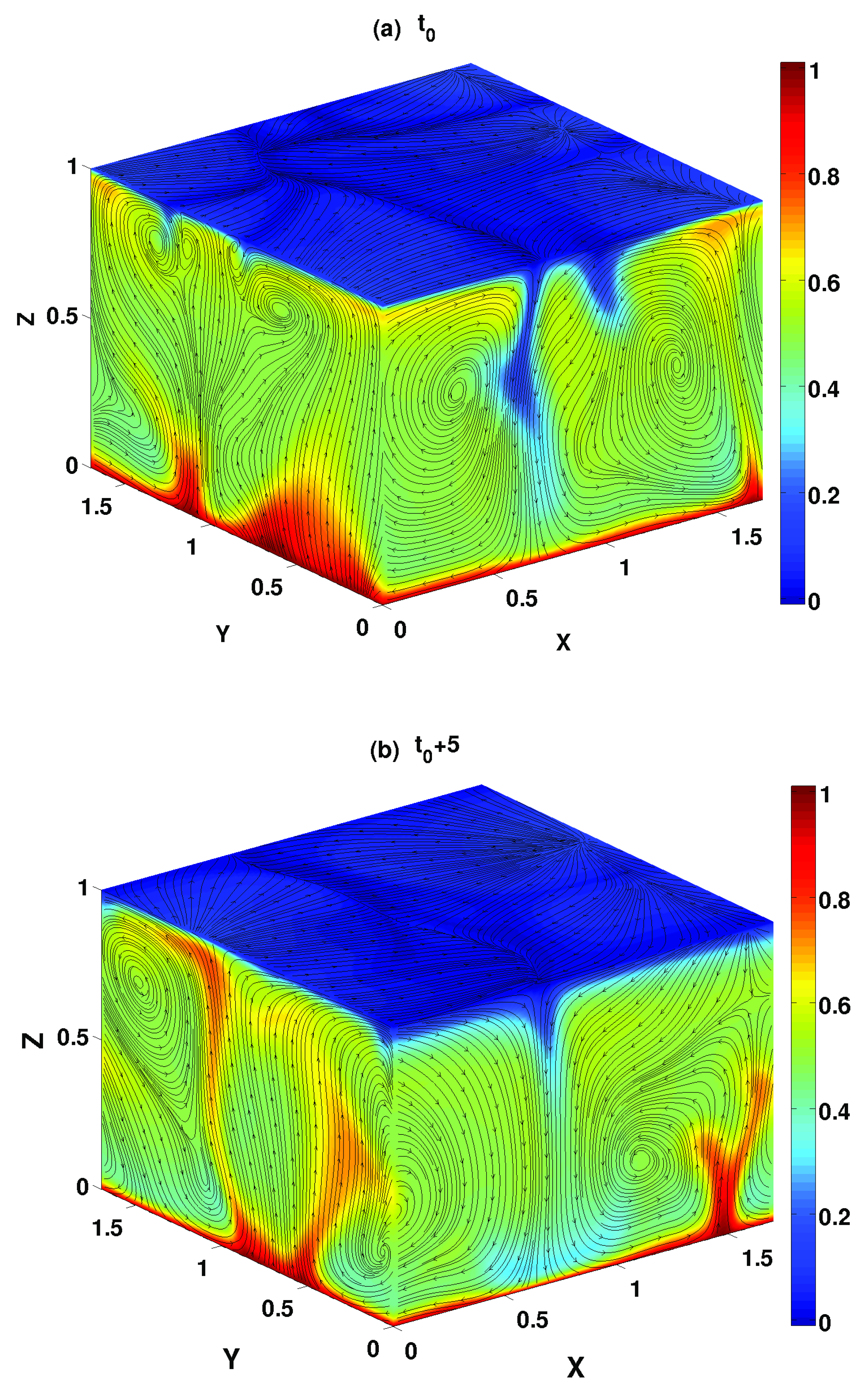Figure 1 shows the combined plot of the total temperature field [$\tilde{T}(x,y,z,t)$] and the velocity field [$\mathsf{v}(x,y,z,t)$] simultaneously at two different instants for a water based nanofluids (${\mathrm{Pr}}_{nf}=6.4$) for ${\mathrm{Ra}}_{nf}=5\times {10}^5$ and ${\mathrm{Q}}_{nf}=100$. The dimensions of the simulation box are $L\times L\times 1$, where $L=\frac{2\pi }{k_c\left({\mathrm{Q}}_{nf}\right)}=1.697$ for ${\mathrm{Q}}_{nf}=100$. The colour bar that is given in each of the viewgraphs shows the temperature field at different points in the convecting fluid. Red, blue, and other colours stand for the hottest, coolest, and intermediate temperatures, respectively. The arrows show the flow directions at the outer surfaces of the simulation box. Thin thermal boundary layers near the lower and upper surfaces of the simulations box are clearly visible. There are generations of thermal plumes (red coloured patches) at the lower boundaries if the temperature gradient is large enough. They are of different sizes and they appear quite irregularly at different locations on the horizontal plate. This also contributes to the fluctuations of fields. There is no viscous boundary layer because of the use of stress-free boundary conditions on the velocity field. Two viewgraphs in Figure 1 confirm the unsteady magnetoconvection. The flow structure is changing with time drastically. Figure 2 shows the variation of flow structures for ${\mathrm{Pr}}_{nf}=6.4$ and ${\mathrm{Ra}}_{nf}=5\times {10}^5$ and for two different values of Chandrasekhar number (${\mathrm{Q}}_{nf}$). Figure 2a shows the total temperature field [$\tilde{T}(x,y,z)$] and the velocity field [$\mathsf{v}(x,y,z)$] in the simulation at a randomly chosen time for ${\mathrm{Q}}_{nf}=100$. The flow structure that is shown in Figure 2b is for ${\mathrm{Q}}_{nf}=250$.

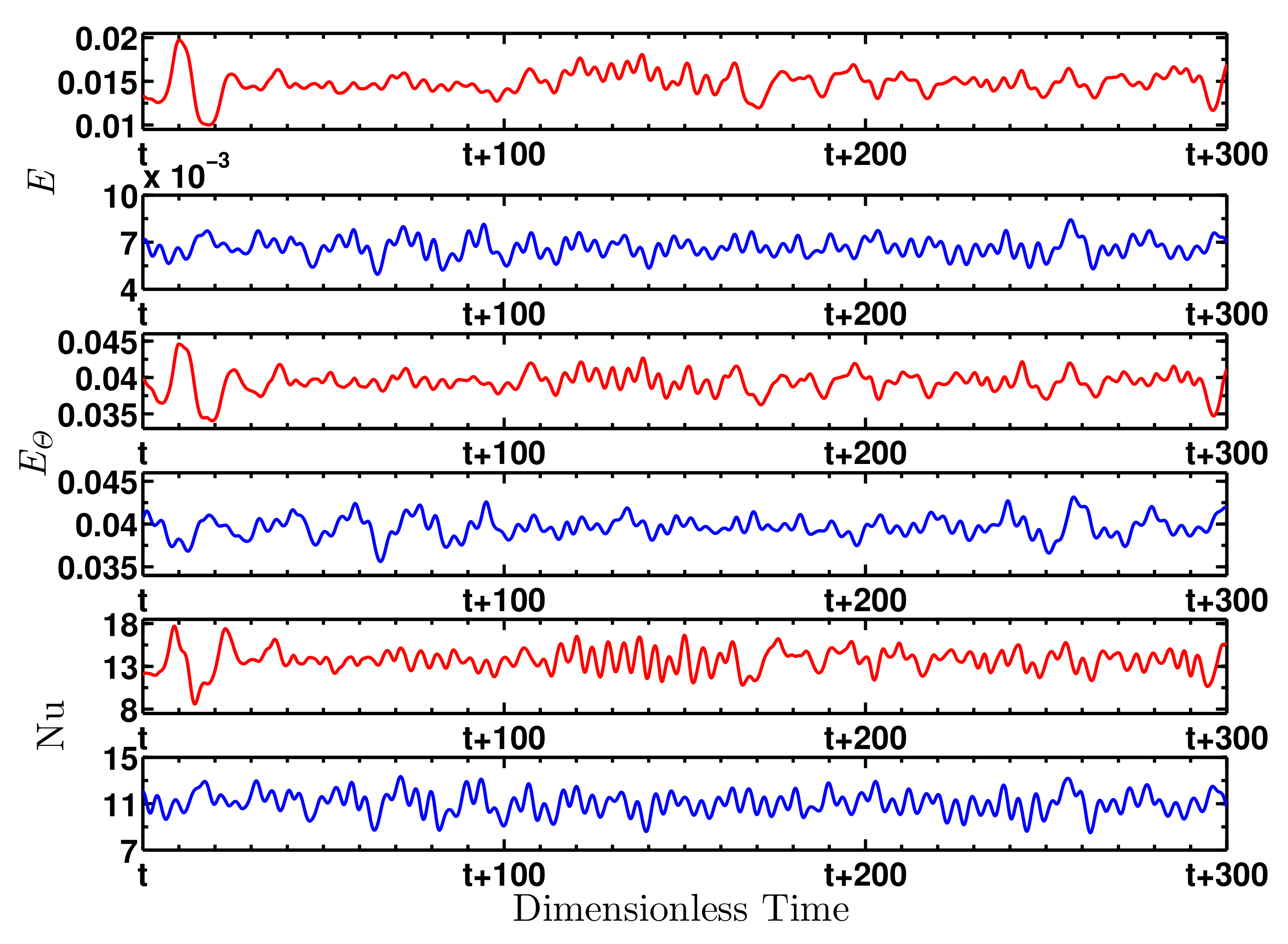
Figure 3 shows the temporal variations of three global quantities for $\mathrm{Ra}=5.0\times {10}^5$, $\mathrm{Pr}=4.0$ and for two different values of $\mathrm{Q}$: (1) the kinetic energy per unit mass (E), (2) the convective entropy per unit mass ($E_{\mathrm{\Theta }}$), and (3) the Nusselt number ($\mathrm{Nu}$). All fields are recorded on all grid points and then the global quantities are computed by averaging over the three-dimensional simulation box. The first two sets of curves (from the top) show the variation of E with dimensionless time for two different values of $\mathrm{Q}$. The red curve is for $\mathrm{Q}=100$ and the blue curve is for $\mathrm{Q}=400$. The energy signal varies irregularly with time. They show appreciable fluctuations. The mean of kinetic energy decreases with increase in $\mathrm{Q}$. The fluctuations of kinetic energy also decreases with an increase in $\mathrm{Q}$. Curves in the third and fourth rows (from the top) show the temporal variation of $E_{\mathrm{\Theta }}$, while curves in the fifth and sixth rows display the temporal signal of $\mathrm{Nu}$. They also vary irregularly with time. The mean values of the convective entropy per unit mass as well as the Nusselt number decrease with an increase in $\mathrm{Q}$. Their fluctuations also decrease, as $\mathrm{Q}$ is raised.

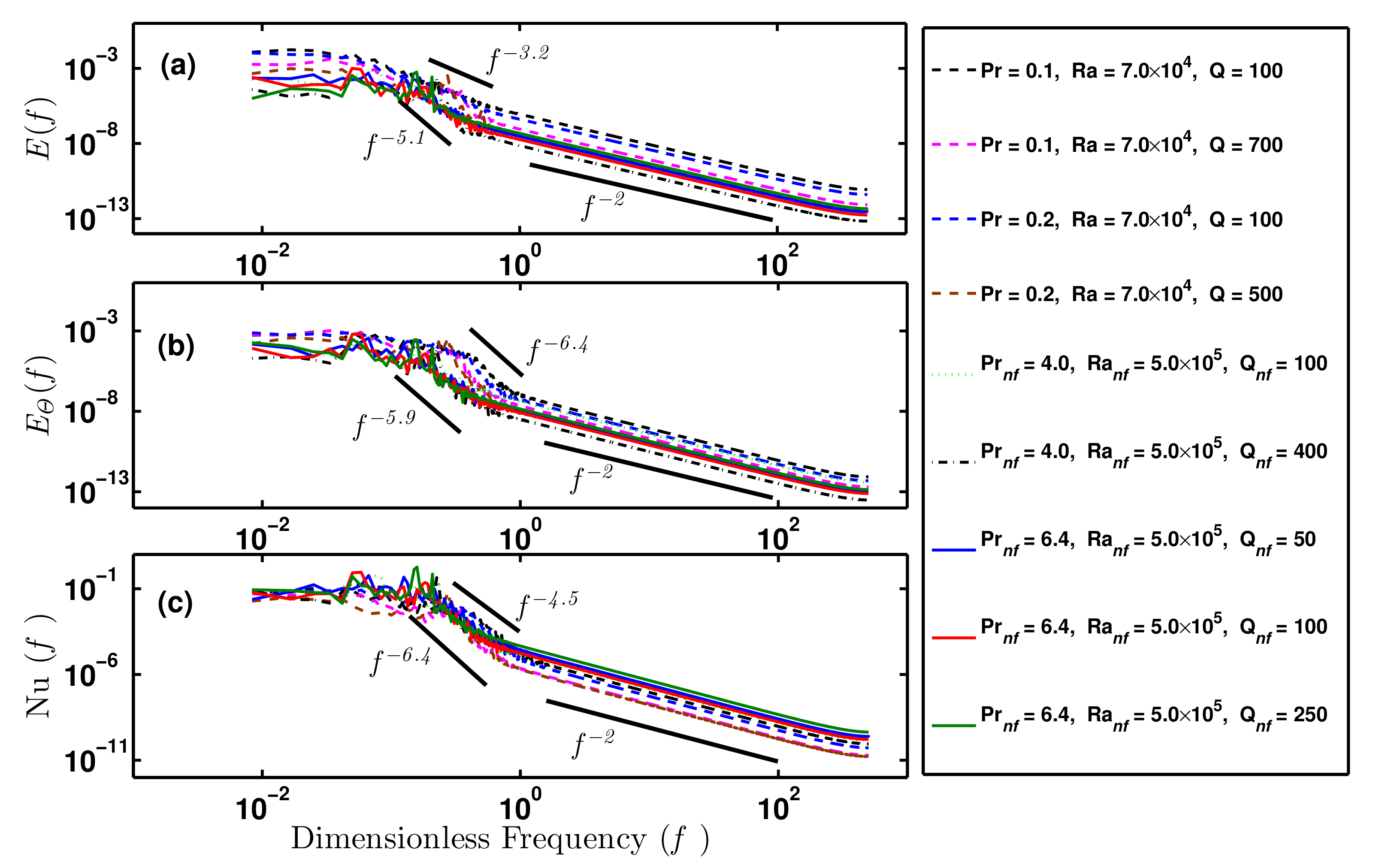
Figure 4 displays the power spectrum densities (PSD) for the global (spatially averaged) quantities in the frequency (f) space for several values of $\mathrm{Ra}$, $\mathrm{Pr}$ and $\mathrm{Q}$. The PSDs of the fluid speed [$E\left(f\right)={\left|\mathrm{v}\left(f\right)\right|}^2$] are shown in Figure 4a. As the thermal energy is injected slowly in the fluid, the spectra show a small slope at low frequencies. In a small frequency window (approximately, $0.04\lesssim f\lesssim 1.0$), the slope of curves $E\left(f\right)-f$ on the log-log scale varies between $-3.2$ to $-5.1$. The energy spectra [$E\left(f\right)$] have more noise in this frequency range. It may be due to irregularity in the size and frequency of thermal plumes from a particular position on the lower boundary. The spectra for nanofluids (${\mathrm{Pr}}_{nf}=4.0$ and $6.4$) show more noise. Smaller values of the thermal diffusivity of the fluid lead to an enhancement of the thermal noise, which makes the spectra nosier at lower frequencies. However, the $E\left(f\right)$ is found to have insignificant noise for $1<f<200$. The frequency spectrum of energy per unit mass [$E\left(f\right)$] decays slowly in this regime. This may be due to the box averaging of the perturbative fields, and it is different than the behaviour near horizontal boundaries. The PSD [$E\left(f\right)$] of the kinetic energy scales with frequency (f) almost as $f^{-\alpha }$ with $\alpha \approx 2$. The scaling behaviour is valid for more than two decades. The PSD shows a clear scaling behaviour for $f>1$. The scaling exponent is independent of $\mathrm{Pr}$, $\mathrm{Ra}$ and $\mathrm{Q}$ in this frequency window.

Table 1. List of Prandtl number $\mathrm{Pr}$, Chandrasekhar number $\mathrm{Q}$, Rayleigh number $\mathrm{Ra}$, exponents of Kinetic energy$\left(\alpha \right)$, exponents of Entropy $\left(\beta \right)$, and exponents of Nusselt number $\left(\gamma \right)$.

$\mathbf{Pr}$	$\mathbf{Ra}$	$\mathbf{Q}$	Exponent $\mathit{\alpha }$	Exponent $\mathit{\beta }$	Exponent $\mathit{\gamma }$
$0.1$	$7.0\times {10}^4$	100	$1.97$	$1.97$	$1.96$
		300	$1.97$	$1.97$	$1.97$
		500	$1.96$	$1.96$	$1.97$
		700	$1.96$	$1.97$	$1.97$
$0.2$	$7.0\times {10}^4$	100	$1.96$	$1.97$	$1.96$
		300	$1.97$	$1.97$	$1.96$
		500	$1.96$	$1.96$	$1.96$
$1.0$	$3.04\times {10}^6$	300	$1.96$	$1.97$	$1.96$
		500	$1.96$	$1.97$	$1.96$
		700	$1.97$	$1.96$	$1.96$
		1000	$1.96$	$1.97$	$1.97$
$2.0$	$3.04\times {10}^6$	500	$1.96$	$1.96$	$1.96$
		700	$1.96$	$1.96$	$1.96$
		1000	$1.96$	$1.97$	$1.96$
$4.0$	$5.0\times {10}^5$	100	$1.96$	$1.97$	$1.96$
		200	$1.96$	$1.97$	$1.97$
		400	$1.96$	$1.97$	$1.97$
$6.4$	$5.0\times {10}^5$	50	$1.96$	$1.97$	$1.96$
		100	$1.97$	$1.97$	$1.96$
		250	$1.97$	$1.96$	$1.97$

gives the numerically computed values of the exponent ($\alpha$) for different values of $\mathrm{Ra}$, $\mathrm{Pr}$, and $\mathrm{Q}$. A similar scaling law [$E\left(f\right)\sim f^{-2}$] was also observed in rotating Rayleigh–Bénard convection [16].

Figure 4b shows the PSDs of the convective entropy [$E_{\mathrm{\Theta }}\left(f\right)={\left|\theta \left(f\right)\right|}^2$] of the fluid in the frequency space for different values of $\mathrm{Ra}$, $\mathrm{Pr}$ and $\mathrm{Q}$. Its power spectra is also noisy in the dimensionless frequency range $0.04<f<1.0$. The slope on the log-log scale varies between $-5.9$ and $-6.4$. However, for $f>1.0$, $E_{\mathrm{\Theta }}$ scales with frequency as $f^{-\beta }$ with $\beta \approx 2$. Table 1 lists the numerically computed values of the exponent $\beta$. Interestingly, the power spectra of the temperature fluctuations are also found to vary as $f^{-2}$ in the rotating RBC experiments [2,16]. The temperature of convecting fluid near the horizontal plates in RBM was measured in experiments on magnetoconvection [17]. The frequency spectra of the temperature field near the horizontal plates vary clearly as $f^{-2}$ for $\mathrm{Q}=0$. Even for very small values of $\mathrm{Q}$ ($\mathrm{Q}\sim {10}^{-3}-{10}^{-4}$), this scaling regime shrinks drastically. The data points for the temperature field were measured locally in this experiment. The frequency spectra of local quantities near the boundary are known to decay faster [5]. The convective entropy is a global quantity and it is computed by taking an average over the simulation box. That is why the power law for the temperature field recorded locally in the experiment [17] may reflect the behaviour in a thin boundary layer near the horizontal plates. In addition, we have used stress-free conditions on the velocity field on the horizontal plates. We only have thermal boundary layers. These may be reasons for disagreement in the power behaviour.

Figure 4c shows the power spectral densities of the thermal flux [Nusselt number, $\mathrm{Nu}\left(f\right)]$ for several values of $\mathrm{Ra}$, $\mathrm{Pr}$, and $\mathrm{Q}$. PSDs of the Nusselt number also show the scaling behaviour. The PSDs are noisy, as in the case of energy and entropy signals, for dimensionless frequencies $0.04<f<1.0$, if $\mathrm{Pr}>1$. The scaling exponent varies between $-4.5$ to $-6.4$ in this frequency window. However, for higher values of dimensionless frequency ($1<f<200$), the spectra for thermal flux [$\mathrm{Nu}\left(f\right)$] also shows very clear scaling: $\mathrm{Nu}\left(f\right)\sim f^{-\gamma }$, with $\gamma \approx 2$. Table 1 shows the values of the exponent $\gamma$ that is computed in DNS. The measurements of the spectra of thermal flux in RBC also shows the similar scaling law [5]. The scaling behaviour for all global quantities for Rayleigh-Bénard magnetoconvection shows a similar power law. This is also observed in experiments in different systems [2,5] as well as in numerical simulations [15,16]. The power spectra of systems showing self-organised criticality [28] scale with frequency as $f^{-1}$, which is different than the scaling behaviour in the hydrodynamic systems discussed here.

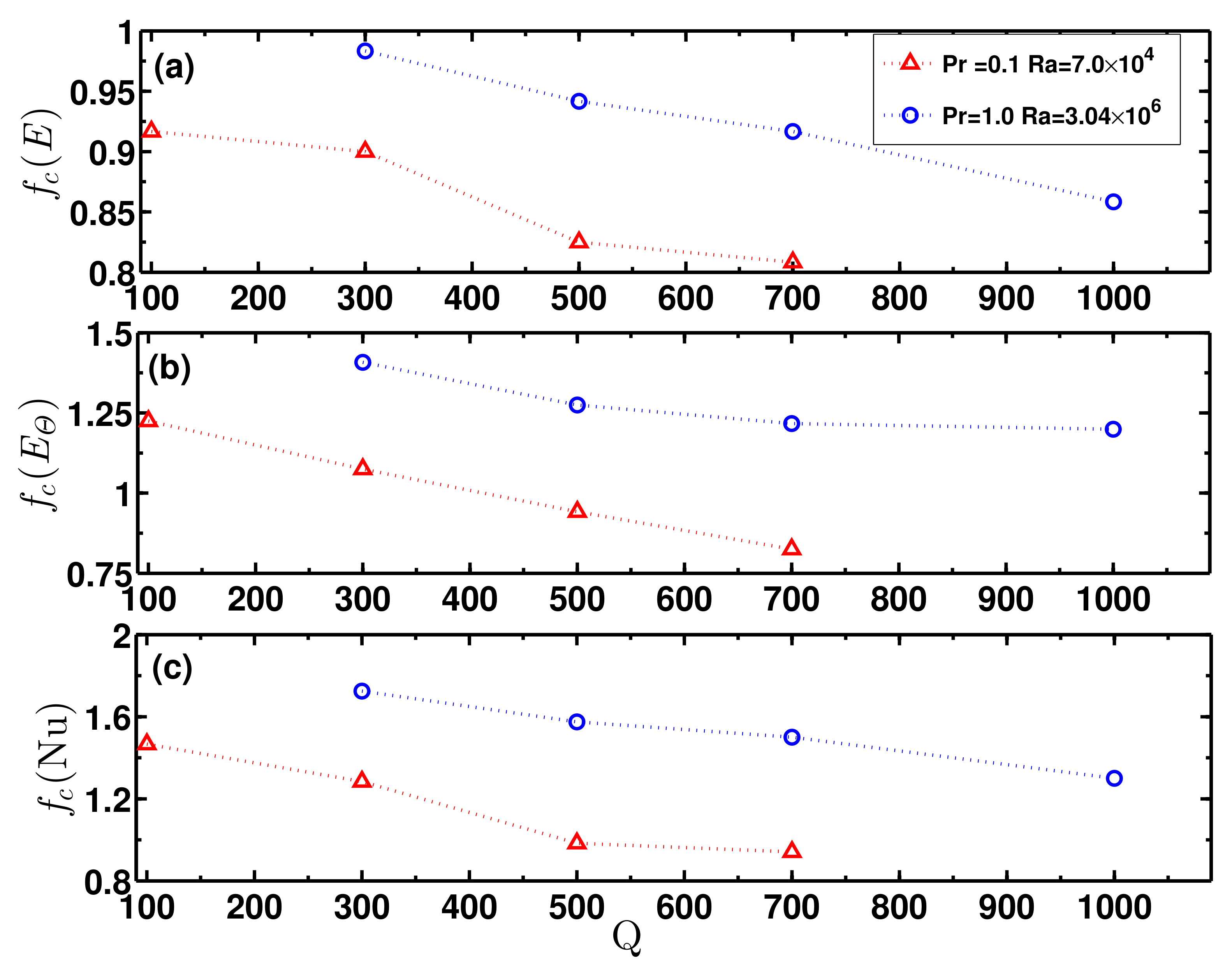
The scaling law showing the variation of the power spectra as $f^{-2}$ starts at a critical frequency ($f_c$) for different values of $\mathrm{Q}$. Figure 5 shows the variation of $f_c$ for $E\left(f\right)$, $E_{\mathrm{\Theta }}\left(f\right)$, and $\mathrm{Nu}\left(f\right)$ with $\mathrm{Q}$ for two different sets of $\mathrm{Ra}$ and $\mathrm{Pr}$. The critical frequency $f_c\left(E\right)$ decreases, as $\mathrm{Q}$ is increased (see Figure 5a). Figure 5b,c show the variations of $f_c\left(E_{\mathrm{\Theta }}\right)$ and $f_c\left(\mathrm{Nu}\right)$, respectively, with $\mathrm{Q}$. The values of critical frequencies are different for $E\left(f\right)$, $E_{\mathrm{\Theta }}\left(f\right)$ and $\mathrm{Nu}\left(f\right)$. However they all decrease with an increase in $\mathrm{Q}$ for given values of $\mathrm{Ra}$ and $\mathrm{Pr}$. A vertical magnetic field is known to delay the onset of fluid flow in RBC [18]. The external magnetic field suppresses the fluid motion, which leads to a decrease in $f_c\left(\mathrm{Q}\right)$, as $\mathrm{Q}$ is raised.

5. Conclusions

The results of DNS on Rayleigh–Bénard magnetoconvection show that frequency spectra of global quantities (the kinetic energy $E\left(f\right)$, convective entropy $E_{\mathrm{\Theta }}\left(f\right)$, and the Nusselt number $\mathrm{Nu}\left(f\right)$) vary differently in different frequency windows. At low frequencies, the thermal energy enters slowly into the moving fluid. The frequency spectra, therefore have a small slope at low frequencies. In a narrow intermediate frequency range, the spectral densities of global quantities decrease sharply with frequency (f). They show power law behaviour. However, the scaling exponents are dissimilar for different global quantities. The energy spectrum [$E\left(f\right)$] varies with the frequency (f) as $E\left(f\right)\sim f^{-\xi }$, with $3.2\le \xi \le 5.1$. Scaling behaviour for the convective entropy and Nusselt number are $E_{\mathrm{\Theta }}\left(f\right)\sim f^{-\eta }$, with $5.9\le \eta \le 6.4$ and $\mathrm{Nu}\left(f\right)\sim f^{-\zeta }$ with $4.5\le \zeta \le 6.4$, respectively. For frequencies above a critical frequency $f_c$, all global quantities show universal scaling behaviour. The critical values $f_c\left(E\right)$, $f_c\left(E_{\mathrm{\Theta }}\right)$, and $f_c\left(\mathrm{Nu}\right)$ are different for kinetic energy, convective entropy, and the Nusselt number, respectively. The spectra of all three global quantities scale with frequency as $f^{-2}$. The scaling exponent of $-2$ at higher frequencies are independent of $\mathrm{Ra}$, $\mathrm{Pr}$, and $\mathrm{Q}$. The scaling behaviour of the global quantities at higher frequencies appears to be a universal feature in turbulent flows. The results that are presented here may also be relevant for some problems of geophysics, water-based nanofluids, crystal growth, and magnetohydrodynamics.