Magnetic Helicity and the Geodynamo

Abstract

We present theoretical and computational results in magnetohydrodynamic turbulence that we feel are essential to understanding the geodynamo. These results are based on a mathematical model that focuses on magnetohydrodynamic (MHD) turbulence, but ignores compressibility and thermal effects, as well as imposing model-dependent boundary conditions. A principal finding is that when a turbulent magnetofluid is in quasi-equilibrium, the magnetic energy in the internal dipole component is equal to the magnetic helicity multiplied by the dipole wavenumber. In the case of the Earth, measurement of the exterior magnetic field gives us, through boundary conditions, the internal poloidal magnetic field. The connection between magnetic helicity and dipole field in the liquid core then gives us the toroidal part of the internal dipole field and a model value of 3 mT for the average core dipole magnetic field. Here, we present the theoretical analysis and numerical simulations that lead to these conclusions. We also test an earlier assertion that differential oblateness may be related to dipole alignment, and while there is an effect, rotation appears to be far more important. In addition, the relationship between dipole quasi-stationarity, broken ergodicity and broken symmetry is clarified. Lastly, we discuss how inertial waves in a rotating magnetofluid can affect dipole alignment.

1. Introduction

Explaining the origin of planetary and stellar magnetic fields has been a scientific quest since Larmor [1] hypothesized that magnetohydrodynamic (MHD) motions within the Sun, and by extension, the Earth, were responsible for the creation and maintenance of global magnetic fields. Numerical simulations of the geodynamo [2,3,4] have established that MHD processes within the Earth are capable of creating magnetic fields similar to the actual geomagnetic field, including reversals of the dominant dipole component.

However successful these numerical simulations were in proving the MHD nature of the geodynamo, the fundamental origin of the dominant, quasi-steady geomagnetic dipole field still remained a mystery [5]. In previous work, we showed that extending the statistical mechanics of ideal MHD turbulence opened the door to understanding the fundamental origin of the geodynamo [6,7] and then demonstrated that these ideal results appeared to apply to real (i.e., forced and dissipative) MHD turbulence [8,9]. In Reference [9], we put forward the hypothesis that differences in the oblateness of the outer and inner boundaries of a spheroidal shell could cause dipole alignment. In the present work, we studied the analogue of this with a Fourier model by using stretching-shrinking factors $q_x$, $q_y$, and $q_z$ ($q_{min}$ is the smallest and $q_{max}$ the largest of these factors). These factors change the relative lengths of the x-, y- and z-directions in both x-space and k-space, as will be described in Section 3.3.

We use a Fourier model as a surrogate for a spherical model because the statistical mechanics of ideal, rotating MHD turbulence are equivalent in the two cases [7]. Both models are based on the MHD equations transformed from physical, or x-space, to a dynamical system of interacting modes in k-space. In either x- or k-space, there is no imposed magnetic field; only overall rotation is imposed. Here, the magnetic field is dynamically generated by MHD turbulence.

We find, in both Fourier and spherical cases, that the largest-scale (smallest wavenumber k) magnetic field modes are very energetic and quasi-steady, i.e., random variables with large mean values subject to only very small fluctuations. The explanation of this is that there is a broken ergodicity: we expected all modes to be fluctuating zero-mean random variables and they mostly are—except for certain largest-scale modes, which will have a very large mean and comparatively very small fluctuations [6]. (Not all of the smallest-k modes need to have the same value—there is a dynamically broken symmetry.) The only requirement for this to occur is that the system have a non-zero magnetic helicity $H_M$. In the case of ideal rotating MHD turbulence, $H_M$ is an integral invariant, along with the energy E. In the forced, dissipative, quasi-equilibrium case, driven so that it has a large, relatively constant $H_M$, behavior is equivalent in that a largest-scale, quasi-steady ‘dipole’ component arises [8,9]. Although the Fourier and spherical models have equivalent ideal statistical mechanics and dynamical evolution in k-space, they appear, of course, very different and are not comparable in x-space, where the largest-scale mode in a periodic box has a sinusoidal shape, while in the spherical case it is a spherical harmonic dipole. (At times, we will refer to the largest-scale mode in the Fourier model as the ‘dipole’, although this is meant figuratively and not meant to imply that the x-space structures are similar, only that the corresponding modes in k-space are equivalent).

The smallest wavenumber k magnetic field quasi-steady mode (or modes) may be thought of as a ‘mean field’, but it is not the mean field that is assumed to exist in ‘mean field electrodynamics’ (MFE) [10]. The a priori MFE mean-field is introduced by altering the magnetic field evolution equation, thereby changing the fundamental nature of the MHD equations; the result is the MFE equations. Instead, basing our work on the MHD equations, we see that a quasi-steady, largest-scale component of the magnetic field emerges dynamically and has an explanation by a statistical mechanics with broken ergodicity and broken symmetry, as will be discussed at length in this paper. Thus, a ‘mean field’ emerges from MHD turbulence, per se, and there is no need to impose one a priori.

Let us add that the interesting question of geomagnetic reversals is not addressed here. This presumably depends on the equilibrium of an existing geomagnetic dipole orientation being destabilized by unseen processes in the Earth’s interior or by some natural bi-stability. Here, we are only concerned with a system that is in a state of equilibrium or quasi-equilibrium and important questions as to the cause of reversals are beyond the scope of this paper.

Our principal result is that without magnetic helicity there is no dipole field. Thus, if the Earth has a dipole field, we require that it have magnetic helicity. In fact, by measuring the strength of the Earth’s external dipole magnetic field and by mapping this mathematically onto the core-mantle boundary, we can estimate the value of the magnetic helicity in the core.

This principal result and all of the related results, we believe, further enhance the view that magnetic helicity and MHD turbulence play essential roles in understanding the fundamental cause of the geodynamo (and perhaps other astrophysical dynamos [11,12]). Next, we briefly review our numerical method, then summarize our new theoretical and computational results, followed by detailed explanations of how they were found.

2. Numerical Procedure

A Fourier spectral transform method [13] on an $N^3$ grid with $N=64$ is used; the minimum wave number is $\underline{k}=q_{min}$ and the maximum wave number is $\overline{k}=30.2q_{max}$. Time-integration is performed with a third-order Adams Bashforth–Adams Moulton method [14] with a time-step of $\Delta t=0.001$; initial magnetic and kinetic energy spectra are $E_M\left(k\right)\sim E_K\left(k\right)\sim k^{4}exp(-k^2/k_{\mathrm{o}}^2)$, where $k_{\mathrm{o}}=6$. Viscosity and magnetic diffusivity are set to zero so that the flow is ideal. (A grid size of ${64}^3$ was used so that the ten runs of

Table 1. Parameters for new ideal MHD turbulence runs, which all had the same constant energy $\mathcal{E}=1$, with less than 0.1% change during a run. The magnetic helicity ${\mathcal{H}}_M$ and ${\mathcal{H}}_C$ are given below and also changed less than 0.1%, except in the runs with ${\mathsf{\Omega }}_{\mathrm{o}}\ne 0$, where ${\mathcal{H}}_C$ fell quickly to ∼0 and fluctuated only slightly thereabout. The runs with cubical grids ($q_x=q_y=q_z=1$) begin with the letter C and those with stretched grids with the letter S. Simulation times were t = 0 to $t_{end}$, with $\Delta t=0.001$. The angular rotation vector of each run is ${\mathsf{\Omega }}_{\mathrm{o}}$, while the stretching factors are $q_x$, $q_y$ and $q_z$ for k-space (and the inverse of these for x-space). $\underline{R}$ is the average of the ratios $R={\mathcal{E}}_M^d/\underline{k}\left|{\mathcal{H}}_M\right|$, which are themselves averages over the last 20% of each run.

Run:	C0	CX	CY	CZ	S10	S20	S30	S1X	S1Y	S1Z
$t_{end}$:	500	400	400	400	500	500	500	400	400	400
$q_x$:	1	1	1	1	0.95	1	$\frac{1}{0.95}$	0.95	0.95	0.95
$q_y$:	1	1	1	1	$\frac{1}{0.95}$	0.95	1	$\frac{1}{0.95}$	$\frac{1}{0.95}$	$\frac{1}{0.95}$
$q_z$:	1	1	1	1	1	$\frac{1}{0.95}$	0.95	1	1	1
${\mathsf{\Omega }}_{\mathrm{o}}$:	0	$10\widehat{\mathbf{x}}$	$10\widehat{\mathbf{y}}$	$10\widehat{\mathbf{z}}$	0	0	0	$10\widehat{\mathbf{x}}$	$10\widehat{\mathbf{y}}$	$10\widehat{\mathbf{z}}$
${\mathcal{H}}_M$	0.1270	0.1307	0.1307	0.1269	0.1271	0.1266	0.1271	0.1271	0.1271	0.1271
${\mathcal{H}}_C$	0.0590	0	0	0	0.0589	0.0588	0.0592	0	0	0
$\overline{R}$:	0.989	0.955	0.967	0.975	1.001	1.000	1.046	0.982	1.072	1.017

could be completed in a reasonable amount of time with the resources available, an 8-core Linux computer, each core running at $\sim 8$ s$/\Delta t$). The integral invariants of ideal MHD turbulence are the volume-averaged energy E and magnetic helicity $H_M$, as well as the cross helicity $H_C$ when there is no rotation. The ideal invariants changed less than 0.1% during the runs of Table 1, while the kinetic helicity $H_K$, though it is an ideal invariant for hydrodynamic turbulence, fell to zero very quickly and had small fluctuations about that value. Further details concerning mathematical modeling and numerical procedure may be found in [6,8,9].

3. Summary of Results

Here, we present a brief summary of the major results to be detailed later in this paper. In what follows, both a Fourier model (periodic box) [9] and a spherical harmonic model (spherical shell) are employed, with the Fourier model serving numerically as a surrogate for the spherical harmonic model. While the periodic box is a 3-torus with no boundaries, the spherical shell model [7] has homogeneous boundary conditions, i.e., the normal components of all fields are zero on the spherical surfaces bounding the internal, turbulent magnetofluid; these boundary conditions were introduced by [15]. Here, these boundaries are not coincident with the Earth’s outer or inner core boundaries (whose precise topography is not well known, anyhow), but are set conceptually inside of them a short distance away at the top of each laminar boundary layer; at the core-mantle boundary (CMB), this laminar layer is estimated to be ∼160 m thick [16] or about 0.07% of the thickness of the outer core. It is within this laminar boundary layer that the magnetic field gains a radial component, eventually becoming the external magnetic field. The external field is connected to the internal, turbulent magnetic field by assuming tangential continuity at the model’s upper boundary. This view of magnetic structure appears to be reflected in Figure 1 of Reference [2]. The efficacy of this model is discussed in Section 3.2, below.

Please note that what is meant by the ‘dipole part’ of a Fourier expansion is comprised of those coefficients that have the smallest wavenumbers. In addition, in regard to the magnetic field, the Fourier coefficients that have positive magnetic helicity are ${\tilde{b}}_{+}\left(\mathbf{k}\right)$ and those with negative magnetic helicity are ${\tilde{b}}_{-}\left(\mathbf{k}\right)$; similarly, the Fourier coefficients that have positive kinetic helicity are ${\tilde{u}}_{+}\left(\mathbf{k}\right)$ and those with negative kinetic helicity are ${\tilde{u}}_{-}\left(\mathbf{k}\right)$. The set of coefficients with the same wavevector $\mathbf{k}$ will be called a ‘Fourier mode’ and the mode $\mathbf{k}$ and the mode $-\mathbf{k}$ are not independent because, for example, ${\tilde{b}}_{+}\left(\mathbf{k}\right)={\tilde{b}}_{+}^{*}(-\mathbf{k})$; coefficients can have the same wavenumber $k=\left|\mathbf{k}\right|$ and there are no coefficients with $k=0$. The number of independent modes for $\underline{k}\le k\le \overline{k}$ is $\mathcal{M}$; in our simulations, $N=64$ and $\mathcal{M}=$ 57,656. In what follows, for definiteness, we choose the global magnetic helicity ${\mathcal{H}}_M$ to be positive. The integral invariants of ideal MHD turbulence are, again, the energy E and magnetic helicity $H_M$, as well as the cross helicity $H_C$ when there is no rotation; these are all volume-averaged quantities as described in Section 5, as are the magnetic energy $E_M$, kinetic energy $E_K$ and related quantities.

3.1. Magnetic Dipole Energy and Magnetic Helicity

The energy in the dipole part of the magnetic field generated by MHD turbulence is equal to the absolute value of the magnetic helicity multiplied by the smallest wavenumber. This result was implicit in our previous formulations [6,7], but further analysis, discussed in more detail in Section 9, reveals that

$${\mathcal{E}}_M^d=\underline{k}\left|{\mathcal{H}}_M\right|.$$

(1)

Here, ${\mathcal{E}}_M^d$ is the expectation value $〈E_M^d〉$ of the dipole magnetic energy and the expectation value of the magnetic helicity is $〈H_M〉={\mathcal{H}}_M$, where ${\mathcal{H}}_M$ is a constant for ideal MHD turbulence; expectation values are defined in Section 6. As discussed in Section 4.2, the smallest possible wavenumber is $\underline{k}$ and is associated with the dipole, while the corresponding wavevector is $\underline{\mathbf{k}}$ (in the symmetric case, there are three of them).

The result (1) has been tested on ten new ideal MHD turbulence Fourier method simulations of Table 1, as well as ten real (forced, dissipative) simulations, drawn from [9] that are given in

Table 2. Forced, dissipative MHD turbulence runs of [9]. Time step was $\Delta t=0.001$ and simulation times were t = 0 to 2500 for the first seven, and t = 2500 to 3500 for the last three. The angular rotation vector of each run is ${\mathsf{\Omega }}_{\mathrm{o}}$, while the stretching factors were all $q_x=q_y=q_z=1$. $\underline{R}$ is the average of $R={\mathcal{E}}_M^d/\underline{k}\left|{\mathcal{H}}_M\right|$, which are themselves averages over the last 20% of each run.

Run:	NM01	NM02	NM03	NM04	NM05	NM06	NM07	NM02c	NM06c	NM08c
$E^{avg}$:	1.0151	1.0644	1.0486	1.0782	1.0404	1.0183	0.9982	1.0427	1.0462	0.9992
$H_M^{avg}$:	0.6251	0.6947	0.8049	0.7119	0.6513	0.6179	0.7118	0.8461	0.8491	0.7079
$H_C^{avg}$:	0.0163	0.0011	−0.0068	−0.0020	−0.0000	−0.0055	−0.0001	−0.0202	0.0059	0.0133
${\mathsf{\Omega }}_{\mathrm{o}}$:	0	0	0	0	$10\widehat{\mathbf{z}}$	$10\widehat{\mathbf{z}}$	$10\widehat{\mathbf{z}}$	0	$10\widehat{\mathbf{z}}$	$10\widehat{\mathbf{z}}$
$\overline{R}$:	1.020	0.997	0.977	0.950	0.918	1.059	0.988	1.000	1.015	1.038

. Let us denote the ratio of the right and left sides of (1) as $R={\mathcal{E}}_M^d/\underline{k}\left|{\mathcal{H}}_M\right|$. Averaging R over the last 20% of each run gives a value $\overline{R}$ for each run, and then averaging the averages $\overline{R}$ gives us a mean ${\overline{R}}_{avg}$ and standard deviation ${\overline{R}}_{std}$ for each of Table 1 and Table 2. Using the notation $\mathcal{R}={\overline{R}}_{avg}\pm {\overline{R}}_{std}$, for the ten runs in Table 1, $\mathcal{R}=1.000\pm 0.036$ and for the ten runs in Table 2, $\mathcal{R}=0.998\pm 0.041$. The significance of Table 2 (real MHD turbulence) is that the values of $\overline{R}$ are commensurate with those found in Table 1 (ideal MHD turbulence), i.e., real and ideal MHD turbulence behave similarly with regard to the theoretical prediction (1).

The prediction (1) can be visually verified, as seen in Figure 1 and Figure 2, where the lowest-wavenumber positive magnetic helicity coefficients ${\tilde{b}}_{+}\left(\underline{\mathbf{k}}\right)$ are normalized by $N^{3/2}$ (since the expectation value of any coefficient’s energy is $〈|{\tilde{b}}_{\pm }{\left(\mathbf{k}\right)|}^2〉/N^3$ or $〈|{\tilde{u}}_{\pm }{\left(\mathbf{k}\right)|}^2〉/N^3$, where $N^3$ is the grid size) and by ${\mathcal{H}}_M$ in accordance with (1); if all dipole coefficients had equal energies, their doubly normalized magnitudes would be $1/\sqrt{3}$ and if one of these coefficients had all the energy predicted by (1), its magnitude would be unity. Thus, the theoretical prediction (1) appears to be well confirmed through the Fourier method (periodic box) numerical simulations of both ideal and real MHD turbulence.

In addition to the energy ${\mathcal{E}}_M^d$ contained in the dipole modes of the magnetic field, given by (1), the rest of the magnetic field has an energy ${\mathcal{E}}_M^h$ (‘h’ stands for higher-wavenumber, non-dipole positive magnetic helicity components, as well as all negative magnetic helicity ones), while the velocity field has kinetic energy ${\mathcal{E}}_K$; the total energy is $\mathcal{E}={\mathcal{E}}_M^d+{\mathcal{E}}_M^h+{\mathcal{E}}_K$. In addition to (1), we find

$${\mathcal{E}}_M^h={\mathcal{E}}_K=\frac{1}{2}(\mathcal{E}-\underline{k}|{\mathcal{H}}_M\left|\right).$$

(2)

The essential result (2), along with (1), is discussed in Section 9. Using (1) and (2), we clearly have $\mathcal{E}={\mathcal{E}}_M^d+{\mathcal{E}}_M^h+{\mathcal{E}}_K$.

Next, we discuss the application of the principal result (1) to the Earth’s outer core. We use the spherical shell model of [7] and assume that ideal results are qualitatively applicable to the low-wavenumber (large length-scale) behavior of a real turbulent magnetofluid. This assumption was tested previously numerically on a Fourier model and seen to be a fairly good one at low wavenumber [9]. Forced, dissipative MHD turbulence behaves very similarly to ideal MHD turbulence at the largest wavelengths and important measures of MHD turbulence are commensurate, as application of the ideal result (1) to forced, dissipative numerical data shows us in Table 2.

3.2. Knowledge of the Internal Toroidal Field

The Fourier model examines MHD turbulence in a periodic box, for which there is no ‘outside’ but only an ‘inside’. Thus, the results above are pertinent to the flow interior to the Earth’s fluid (outer) core. We have considered MHD turbulence in the outer core by developing a spherical shell model that uses spherical Bessel function-spherical harmonic expansions and have found that the statistical theory of ideal MHD turbulence developed for the Fourier model system also applies to this case [7]. In this spherical shell model, there are poloidal $a_{lmn}$ and toroidal $b_{lmn}$ magnetic field coefficients, and it is the poloidal coefficients $a_{lmn}$ that can be matched to the Gauss coefficients $g_l^m$ and $h_l^m$ at the outer boundary of the numerical model. The toroidal coefficients $b_{lmn}$ are internal to the outer core and it had long been assumed that these were unknowable. However, consider the following results.

A turbulent magnetofluid in the rotating spherical shell model of [7] has the ideal invariants energy $\mathcal{E}$, where $\mathcal{E}={\mathcal{E}}_M+{\mathcal{E}}_K$, and magnetic helicity ${\mathcal{H}}_M$. In that model, the magnetic energy ${\mathcal{E}}_M$ and helicity ${\mathcal{H}}_M$ are given by

$$\begin{array}{ccc}\hfill {\mathcal{E}}_M& =& \frac{1}{2}\sum _{l,m,n}\left(|b_{lmn}{|}^2+k_{ln}^2{\left|a_{lmn}\right|}^2\right),\hfill \\ \hfill \end{array}$$

(3)

$$\begin{array}{ccc}\hfill {\mathcal{H}}_M& =& \sum _{l,m,n}{a}_{lmn}^{*}{b}_{lmn}.\hfill \end{array}$$

(4)

The indices l and m are the degree and order of a spherical harmonic $Y_l^m(\theta ,\varphi )$, and n denotes the nth zero $k_{ln}$ of ${\widehat{g}}_l\left(k_{ln}r\right)$ at $r=1$, where ${\widehat{g}}_l\left(k_{ln}r\right)$ is a linear combination of spherical Bessel and Neumann functions. Please see [7] for more details; in that paper, the smallest spherical shell dimensionless wavenumber for an Earth-like model is $\underline{k}=k_{11}\cong 1.8638$ (the next smallest wavenumber is $k_{21}\cong 2.1497$). The spherical shell version of (1) is

$${\mathcal{E}}_M^d=k_{11}\left|{\mathcal{H}}_M\right|.$$

(5)

The geomagnetic field is measured at the surface out to spherical harmonic degree $l=13$ [17], where about 93% of the magnetic energy at the Earth’s surface is in the dipole, $l=1$. However, at the CMB, only about 38% of its magnetic energy is locked up in the dipole $l=1$ components; this percentage is probably high, as there is presumably more energy that is unaccounted for in the $l>13$ components. The dipole’s Gauss coefficients $g_1^m$ and $h_1^m$ given by [17] indicate that 97% of the dipole’s energy is held by $g_1^0$, so the dipole moment is closely aligned with the rotation axis.

Theoretically, we expect that the components $a_{1m1}$ and $b_{1m1}$ that have the smallest wave number $\underline{k}=k_{11}$ contribute most to ${\mathcal{H}}_M$ in (4) [7]. Truncating the summations (3) and (4) to the $l=1$ and $n=1$ terms and setting $|{\mathcal{H}}_M|=+{\mathcal{H}}_M$, for ${\mathcal{H}}_M>0$, we have

$$\sum _{m=-1}^1{\left(b_{1m1}-k_{11}{a}_{1m1}\right)}^2=0.$$

(6)

Therefore, if we know the major part of the poloidal dipole magnetic field, then we also know the major part of the toroidal dipole field:

$$b_{1m1}=k_{11}{a}_{1m1}.$$

(7)

Note that, if we had set $|{\mathcal{H}}_M|=-{\mathcal{H}}_M$, the result would be $b_{1m1}=-k_{11}{a}_{1m1}$.

The important point here is that because we can relate the coefficients $a_{1m1}$ to the Gauss coefficients $g_1^m$ and $h_1^m$ through the boundary conditions, we know both the poloidal coefficients $a_{1m1}$ and, through (7), the toroidal coefficients $b_{1m1}$ in the outer core. Using the results in References [7,17], we find, with ${\mathcal{H}}_M>0$,

$$b_{101}=k_{11}{a}_{101}=2C{g}_1^0,b_{111}=k_{11}{a}_{111}=-C(g_1^1-i{h}_1^1).$$

(8)

Formulas in Reference [7] tell us that the conversion factor is $C\cong 19.5$ for degree $l=1$, leading to an estimated mean value of the dipole magnetic field in the outer core of 3.02 mT, or 11.7 times that of average geomagnetic dipole field at the CMB, which is 0.259 mT, based on the 2015 International Geomagnetic Reference Field (IGRF) coefficients [17]. Although the value of 3.02 mT comes from a model with homogeneous boundary conditions [7], the model appears to have some robustness because 3.02 mT is compatible with the value of 2.5 mT estimated by [18] as the mean strength of the total magnetic field in the Earth’s outer core. In addition, the IGRF data tells us that ${\mathcal{E}}_M^d=45.7$ J/m${}^3$ and ${\mathcal{H}}_M=24.5$ J/m${}^2$.

In the case of the dipole, $l=1$, using $k_{11}$ is appropriate because it is the minimum wavenumber $\underline{k}$ of the spherical shell model. However, for estimating higher multipole ($l\ge 2$) field strengths, it is unclear which wavenumber $k_{ln}$, or even how many, to use because the IGRF field components are indexed by degree l and order m, and, in the spherical shell model of [7], there are many wavenumbers $k_{ln}$ associated with each spherical harmonic degree l, but, at present, no obvious procedure for picking out which ones are important.

3.3. Differential Oblateness vs. Rotation in Dipole Alignment

In Reference [9], we put forward the idea that a greater oblateness of the inner core boundary (ICB) with respect to the CMB in the z-direction might influence dipole alignment. In the Fourier case, the analogy is that the periodic box would be stretched in the z-direction compared to the x- and y-directions in x-space; in k-space, this would entail a shrinking in the $k_z$-direction compared to the $k_x$ and $k_y$-directions (or some permutation of this). Thus, $k_j\to q_j{k}_j$, $j=x,y,z$, while $x\to x/q_x$, $y\to y/q_y$ and $z\to z/q_z$. A number of runs were performed, using various values of $q_x$, $q_y$ and $q_z$, with $q_x{q}_y{q}_z=1$, as Table 1 shows. In a numerical simulation with ${\mathcal{H}}_M>0$, the effect of making one of the $q_j$ smaller than the others is to give the positive magnetic helicity Fourier coefficient, say ${\tilde{b}}_{+}\left(q_x\widehat{\mathbf{x}}\right)$ with smallest wave number $k=q_x=q_{min}$, more energy than it would have if all the $q_j=1$; the reason for this is discussed in Section 8.

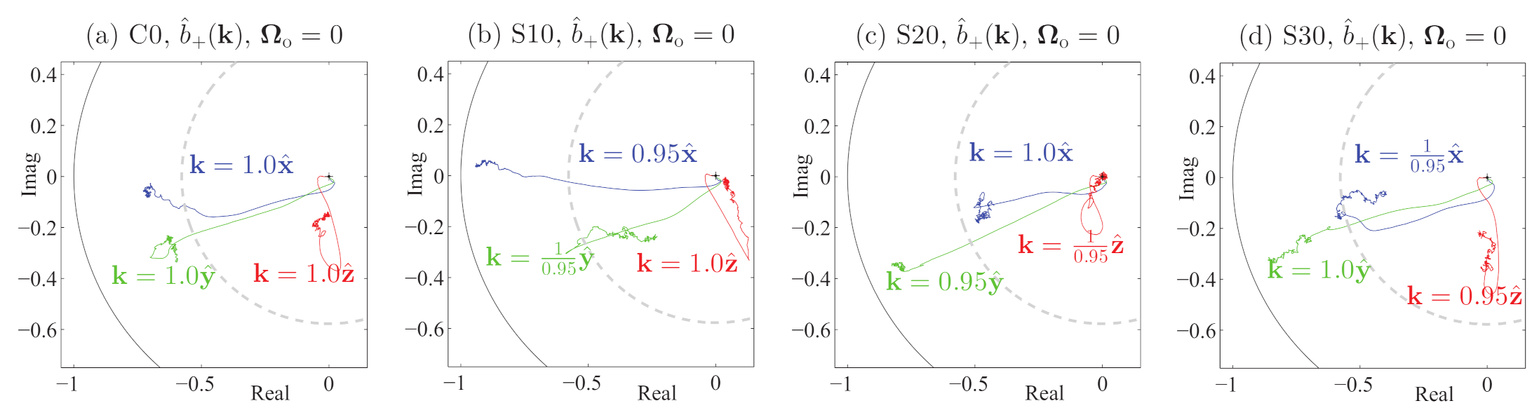
Let us again compare the evolution of the ${\tilde{b}}_{+}(\mathbf{k},t)$, $q_{min}\le k\le q_{max}$, for the four runs C0, S10, S20, and S30 of Table 1. This comparison is made using the trajectories shown in Figure 1, where we plot the real vs. imaginary parts of the doubly normalized ${\tilde{b}}_{+}(\mathbf{k},t)$. In Figure 1, we see that, when the smallest wavevector is in the (b) x-, (c) y- or (d) z-directions, it induces an increase in the magnitude of the corresponding ${\tilde{b}}_{+}(\mathbf{k},t)$ compared to (a), where all $q_j=1$. Although it was initially assumed that all coefficients would be zero-mean random variables [19,20], we clearly see ‘broken ergodicity,’ a concept defined by [21]. Broken ergodicity in MHD turbulence was first noted by [22]; in Figure 1, the phenomenon of ‘broken symmetry’ [23] also appears, in that nonlinear evolution can lead to a lack of equipartition even in the $q_x=q_y=q_z=1$ run C0.

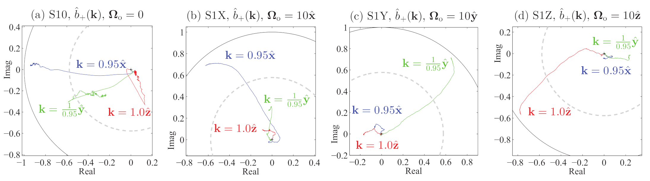
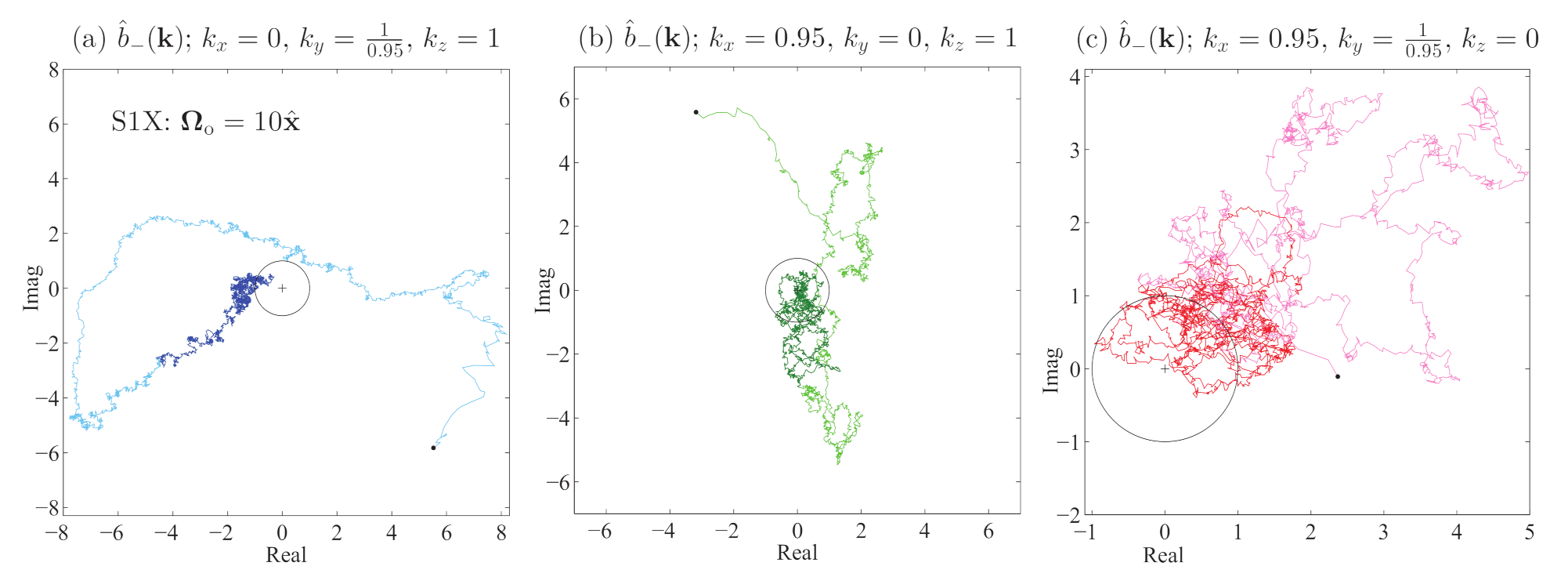
Next, consider Figure 2 where (a) pertains to reference run S10 and Figure 2b–d, which pertain to three runs whose parameters in Table 1 are the same as run S10, except that they have an imposed rotation: in Figure 2b, S1X has ${\mathsf{\Omega }}_{\mathrm{o}}=10\widehat{\mathbf{x}}$, in (c), S1Y has ${\mathsf{\Omega }}_{\mathrm{o}}=10\widehat{\mathbf{y}}$ and in (d), S1Z has ${\mathsf{\Omega }}_{\mathrm{o}}=10\widehat{\mathbf{z}}$. Figure 2 shows that the effect of rotation overrides the effect of differential oblateness. The low-wavenumber, positive magnetic helicity coefficients ${\tilde{b}}_{+}\left(\mathbf{k}\right)$ with $\mathbf{k}$ parallel to ${\mathsf{\Omega }}_{\mathrm{o}}$ develop much greater magnitude than those with $\mathbf{k}$ perpendicular to ${\mathsf{\Omega }}_{\mathrm{o}}$. We discuss a possible reason for this in Section 3.5 below.

3.4. Broken Ergodicity and Broken Symmetry

Figure 1 and Figure 2 show that the dipole components ${\tilde{b}}_{+}\left(\underline{\mathbf{k}}\right)$ exhibit quasi-stationarity, i.e., coherent structure due to broken ergodicity and broken symmetry. We discuss these phenomena in greater detail in Section 10. We believe we have a clearer understanding of their relationship and wish to summarize this here.

Assume $q_x=q_y=q_z=1$ and define a vector ${\tilde{\mathsf{v}}}_d$ in a 3D complex space by

$${\tilde{\mathsf{v}}}_d^T=N^{-3/2}\left[{\tilde{b}}_{+}\left(\widehat{\mathbf{x}}\right){\tilde{b}}_{+}\left(\widehat{\mathbf{y}}\right){\tilde{b}}_{+}\left(\widehat{\mathbf{z}}\right)\right]$$

(9)

This has the dot product $|{\tilde{\mathsf{v}}}_d{|}^2={\tilde{\mathsf{v}}}_d^{†}{\tilde{\mathsf{v}}}_d=\left|{\mathcal{H}}_M\right|$. At least one of the components of ${\tilde{\mathsf{v}}}_d$ will have a large mean value of magnitude $\sim \sqrt{|{\mathcal{H}}_M|}$ that is much larger than the fluctuations it experiences, which are O$\left({\mathcal{M}}^{-1/2}\right)$. The ‘dipole vector’ ${\tilde{\mathsf{v}}}_d$ will thus evolve to become quasi-stationary and, while the expectation value $〈{\tilde{\mathsf{v}}}_d〉$ is zero, the time-average of ${\tilde{\mathsf{v}}}_d$ is almost constant and has a magnitude $\sim {\mathcal{M}}^{1/2}$ greater than its standard deviation, as is seen in Figure 1. This is the origin of broken ergodicity.

The phase space of independent Fourier components can also be subject to an arbitrary unitary transformation. While the choice of a particular set of initial conditions leads to a specific direction for the quasi-stationary vector ${\tilde{\mathsf{v}}}_d$, a unitary transformation can be made so as to point it in any direction we chose: The canonical ensemble represents all directions, which average to zero, but the dynamical system can only evolve so that ${\tilde{\mathsf{v}}}_d$ points in one direction. This is the origin of broken symmetry.

Rotation, however, induces dipole alignment, though the reason why is not yet completely clear.

3.5. Rotation and Dipole Alignment

As mentioned above and shown in Figure 1, differential oblateness can cause alignment, but, as shown in Figure 2, rotation appears to be the absolute controlling factor. The rotation vector ${\mathsf{\Omega }}_{\mathrm{o}}$ enters explicitly into the basic equations only in the velocity Equation (10) and not in the magnetic induction Equation (11). However, it does enter into the magnetic induction equation implicitly through the electromotive field $\mathbf{E}=-\mathbf{u}\times \mathbf{b}$ because of the hydrodynamic inertial waves present in the velocity field $\mathbf{u}$ of a rotating system. While our discussion here will be brief, inertial waves, both Alfvén and hydrodynamic, are well known to be important in planetary cores, as discussed in detail by [24] and [25], respectively.

Here, we examine the inertial wave effects in the context of our Fourier model system. Since inertial waves may introduce a sinusoidal time variation into the electromotive field, the evolution of some of the Fourier magnetic dipole modes can be influenced: if ${\mathsf{\Omega }}_{\mathrm{o}}={\mathsf{\Omega }}_{\mathrm{o}}\widehat{\mathbf{z}}$, then ${\tilde{b}}_{+}\left(\widehat{\mathbf{x}}\right)$ and ${\tilde{b}}_{+}\left(\widehat{\mathbf{y}}\right)$ are strongly affected, while ${\tilde{b}}_{+}\left(\widehat{\mathbf{z}}\right)$ is not affected at all, to leading order in ${\mathcal{M}}^{1/2}$. A qualitative appraisal is given more detail in Section 11.

4. Mathematical Model

4.1. Basic Equations

The non-dimensional form of the 3D incompressible MHD equations in a rotating frame of reference with constant angular velocity ${\mathsf{\Omega }}_{\mathrm{o}}$ can be written as

$$\begin{array}{ccc}\hfill \frac{\partial \mathbf{\omega }}{\partial t}& =& \nabla \times \left[\mathbf{u}\times \left(\mathbf{\omega }+2{\mathsf{\Omega }}_{\mathrm{o}}\right)+\mathbf{j}\times \mathbf{b}\right]+\nu {\nabla }^2\mathbf{\omega },\hfill \\ \hfill \end{array}$$

(10)

$$\begin{array}{ccc}\hfill \frac{\partial \mathbf{b}}{\partial t}& =& \nabla \times \left[\mathbf{u}\times \mathbf{b}\right]+\eta {\nabla }^2\mathbf{b}.\hfill \end{array}$$

(11)

These are described, for example, by References [26,27]. Here, $\mathbf{u}(\mathbf{x},t)$ and $\mathbf{b}(\mathbf{x},t)$ are the turbulent velocity and magnetic fields, respectively. The velocity and magnetic fields are solenoidal: $\nabla ·\mathbf{u}=\nabla ·\mathbf{b}=0$, as are the vorticity $\mathbf{\omega }(\mathbf{x},t)$ and electric current density $\mathbf{j}(\mathbf{x},t)$, defined by

$$\mathbf{\omega }=\nabla \times \mathbf{u},\mathbf{j}=\nabla \times \mathbf{b}.$$

(12)

Non-dimensional density does not appear in (10) because it equals unity. The symbols $\nu$ in (10) and $\eta$ in (11) are shorthand for $1/R_E$ and $1/R_M$, i.e., the inverses of the kinetic and magnetic Reynolds numbers, respectively. In the dimensional form of the equations, $\nu$ is the kinematic viscosity, while $\eta$ is the magnetic diffusivity; $\nu =\eta =0$ for ideal MHD turbulence.

4.2. Fourier Representation

Discrete Fourier transforms for $\mathbf{u}$ and $\mathbf{b}$, connecting x-space (with vectors $\mathbf{x}$) to k-space (with vectors $\mathbf{k}$), are

$$\begin{array}{ccc}\hfill \left[\begin{array}{c}\mathbf{u}(\mathbf{x},t)\hfill \\ \mathbf{b}(\mathbf{x},t)\hfill \end{array}\right]& =& \sum _{\mathbf{k}}\left[\begin{array}{c}\tilde{\mathbf{u}}(\mathbf{k},t)\\ \tilde{\mathbf{b}}(\mathbf{k},t)\end{array}\right]\frac{exp\left(i\mathbf{x}·\mathbf{k}\right)}{N^{3/2}},\hfill \\ \hfill \end{array}$$

(13)

$$\begin{array}{ccc}\hfill \left[\begin{array}{c}\tilde{\mathbf{u}}(\mathbf{k},t)\hfill \\ \tilde{\mathbf{b}}(\mathbf{k},t)\hfill \end{array}\right]& =& \sum _{\mathbf{x}}\left[\begin{array}{c}\mathbf{u}(\mathbf{x},t)\\ \mathbf{b}(\mathbf{x},t)\end{array}\right]\frac{exp\left(-i\mathbf{x}·\mathbf{k}\right)}{N^{3/2}}.\hfill \end{array}$$

(14)

Here, N is the number of grid points in each x-space dimension. Note that the reality of $\mathbf{u}(\mathbf{x},t)$ and $\mathbf{b}(\mathbf{x},t)$ imply that $\tilde{\mathbf{u}}(\mathbf{k},t)={\tilde{\mathbf{u}}}^{*}(-\mathbf{k},t)$ and $\tilde{\mathbf{b}}(\mathbf{k},t)={\tilde{\mathbf{b}}}^{*}(-\mathbf{k},t)$.

Although the periodic box of the model system is usually taken to be a cube, here we will allow for the possibility that it might be elongated or compressed differently in the x-, y-, and z-directions; this simulates the difference in oblateness that may occur in the Earth’s inner and outer cores and might have dynamical importance [9]. To accomplish this elongation or compression, we define $\mathbf{x}$ and $\mathbf{k}$ by

$$\begin{array}{ccc}& & \mathbf{x}=x\widehat{\mathbf{x}}+y\widehat{\mathbf{y}}+z\widehat{\mathbf{z}}=\frac{2\pi }{N}\left(\frac{n_x}{q_x}\widehat{\mathbf{x}}+\frac{n_y}{q_y}\widehat{\mathbf{y}}+\frac{n_z}{q_z}\widehat{\mathbf{z}}\right),\hfill \\ \hfill \end{array}$$

(15)

$$\begin{array}{ccc}& & \mathbf{k}=k_x\widehat{\mathbf{x}}+k_y\widehat{\mathbf{y}}+k_z\widehat{\mathbf{z}}=q_x{m}_x\widehat{\mathbf{x}}+q_y{m}_y\widehat{\mathbf{y}}+q_z{m}_z\widehat{\mathbf{z}}.\hfill \end{array}$$

(16)

The components $n_j$ and $m_j$, $j=x,y,z$, are integers. The $n_j$ satisfy $0\le n_j<N$, while the integers $m_j$ lie in the range $-N/2+1$ and $+N/2$; thus, there are $N^3$ points in both spaces. No matter what the parameters $q_j>0$ are, the dot product $\mathbf{k}·\mathbf{x}$ in Equations (13) and (14) is then always

$$\mathbf{k}·\mathbf{x}=\frac{2\pi }{N}\left(n_x{m}_x+n_y{m}_y+n_z{m}_z\right).$$

(17)

The Fourier transforms (13) and (14) are thus unaffected by the parameters $q_j$, $j=x,y,z$. Here, we will choose $q_x{q}_y{q}_z=1$ so that the volume of the periodic box does not change even when any of the $q_j\ne 1$.

For computational purposes, we define the following vectors with integer components defined above:

$$\mathbf{n}=n_x\widehat{\mathbf{x}}+n_y\widehat{\mathbf{y}}+n_z\widehat{\mathbf{z}},\mathbf{m}=m_x\widehat{\mathbf{x}}+m_y\widehat{\mathbf{y}}+m_z\widehat{\mathbf{z}}.$$

(18)

The Fourier coefficients $\tilde{\mathbf{u}}(\mathbf{k},t)$ and $\tilde{\mathbf{b}}(\mathbf{k},t)$ are nonzero only for $1\le \left|\mathbf{m}\right|\le M<N/2$. The exact value of M is set by a de-aliasing requirement of [28]: $M^2$ is the largest integer such that $M^2\le 2N^2/9$. (Note: Although we will use k as the magnitude of $\mathbf{k}$, we will not use n as the magnitude of $\mathbf{n}$, nor m as the magnitude of $\mathbf{m}$ because we will use n and m as general indices that appear in various mathematical terms).

Let $q_{min}$ equal the smallest of $q_x$, $q_y$, and $q_z$, and let $q_{max}$ be the largest; then, the largest length-scale corresponds to smallest wavenumber $\underline{k}=q_{min}$, associated with $\mathbf{k}=\underline{\mathbf{k}}$, and the smallest length-scale to then largest wavenumber $\overline{k}=q_{max}M$, associated with $\mathbf{k}=\overline{\mathbf{k}}$. Dynamically interacting coefficients fit within a sphere in $\mathbf{m}$-space (ellipsoid in k-space); all coefficients outside this $\mathbf{m}$-sphere, as well as at $\mathbf{m}=0$, are initially zero and remain so during any numerical simulation. Since $\tilde{\mathbf{u}}(\mathbf{k},t)={\tilde{\mathbf{u}}}^{*}(-\mathbf{k},t)$ and $\tilde{\mathbf{b}}(\mathbf{k},t)={\tilde{\mathbf{b}}}^{*}(-\mathbf{k},t)$, only half of the $\mathbf{m}$ that satisfy $1\le \left|\mathbf{m}\right|\le M$ identify independent coefficients. Therefore, the number of independent modes $\mathbf{k}$ is $\mathcal{M}\cong 2\pi M^3/3$; here, for $N=64$, $\mathcal{M}\cong$ 57,515, while the actual numerical count is $\mathcal{M}=$ 57,656.

In k-space, the requirements $\nabla ·\mathbf{u}=\nabla ·\mathbf{b}=0$ become $i\mathbf{k}·\tilde{\mathbf{u}}(\mathbf{k},t)=i\mathbf{k}·\tilde{\mathbf{b}}(\mathbf{k},t)=0$. Thus, $\tilde{\mathbf{u}}(\mathbf{k},t)$ and $\tilde{\mathbf{b}}(\mathbf{k},t)$ have two independent complex vector coefficients each, which can be defined as follows: First, determine a coordinate system for each $\mathbf{k}$ by starting with a unit vector ${\widehat{\mathbf{e}}}_3\left(\mathbf{k}\right)=\mathbf{k}/k=\widehat{\mathbf{k}}$; then choosing a unit vector ${\widehat{\mathbf{e}}}_1\left(\mathbf{k}\right)$ orthogonal to ${\widehat{\mathbf{e}}}_3\left(\mathbf{k}\right)$, and then the remaining unit vector ${\widehat{\mathbf{e}}}_2\left(\mathbf{k}\right)$ is a vector product of the first two, forming a right-handed orthonormal basis for each $\mathbf{k}$:

$$\begin{array}{ccc}{\widehat{\mathbf{e}}}_1\left(\mathbf{k}\right)·{\widehat{\mathbf{e}}}_3\left(\mathbf{k}\right)=0,\hfill & \hfill & {\widehat{\mathbf{e}}}_2\left(\mathbf{k}\right)={\widehat{\mathbf{e}}}_3\left(\mathbf{k}\right)\times {\widehat{\mathbf{e}}}_1\left(\mathbf{k}\right),\hfill \\ \hfill \\ {\widehat{\mathbf{e}}}_i\left(\mathbf{k}\right)·{\widehat{\mathbf{e}}}_j\left(\mathbf{k}\right)={\delta }_{ij},\hfill & \hfill & {\widehat{\mathbf{e}}}_1\left(\mathbf{k}\right)·{\widehat{\mathbf{e}}}_2\left(\mathbf{k}\right)\times {\widehat{\mathbf{e}}}_3\left(\mathbf{k}\right)=1.\hfill \end{array}$$

(This is similar to a Craya–Herring decomposition [29]). Explicit choices [30] for any of the ${\widehat{\mathbf{e}}}_j\left(\mathbf{k}\right)$ will be mentioned as needed.

In terms of the ${\widehat{\mathbf{e}}}_j\left(\mathbf{k}\right)$ defined above, the Fourier vector coefficients $\tilde{\mathbf{u}}\left(\mathbf{k}\right)$ and $\tilde{\mathbf{b}}\left(\mathbf{k}\right)$ are

$$\begin{array}{ccc}\hfill \tilde{\mathbf{u}}(\mathbf{k},t)& =& {\tilde{u}}_1(\mathbf{k},t){\widehat{\mathbf{e}}}_1\left(\mathbf{k}\right)+{\tilde{u}}_2(\mathbf{k},t){\widehat{\mathbf{e}}}_2\left(\mathbf{k}\right),\hfill \\ \hfill \end{array}$$

(19)

$$\begin{array}{ccc}\hfill \tilde{\mathbf{b}}(\mathbf{k},t)& =& {\tilde{b}}_1(\mathbf{k},t){\widehat{\mathbf{e}}}_1\left(\mathbf{k}\right)+{\tilde{b}}_2(\mathbf{k},t){\widehat{\mathbf{e}}}_2\left(\mathbf{k}\right).\hfill \end{array}$$

(20)

However, an equivalent, but more efficacious helical representation can be used:

$$\begin{array}{ccc}\hfill \tilde{\mathbf{u}}(\mathbf{k},t)& =& {\tilde{u}}_{+}(\mathbf{k},t){\widehat{\mathbf{e}}}_{+}\left(\mathbf{k}\right)+{\tilde{u}}_{-}(\mathbf{k},t){\widehat{\mathbf{e}}}_{-}\left(\mathbf{k}\right),\hfill \\ \hfill \end{array}$$

(21)

$$\begin{array}{ccc}\hfill \tilde{\mathbf{b}}(\mathbf{k},t)& =& {\tilde{b}}_{+}(\mathbf{k},t){\widehat{\mathbf{e}}}_{+}\left(\mathbf{k}\right)+{\tilde{b}}_{-}(\mathbf{k},t){\widehat{\mathbf{e}}}_{-}\left(\mathbf{k}\right).\hfill \end{array}$$

(22)

Here, the positive and negative helicity unit vectors and components are

$$\begin{array}{ccc}\hfill {\widehat{\mathbf{e}}}_{\pm }\left(\mathbf{k}\right)& =& \frac{1}{\sqrt{2}}\left[{\widehat{\mathbf{e}}}_1\left(\mathbf{k}\right)\pm i{\widehat{\mathbf{e}}}_2\left(\mathbf{k}\right)\right],\hfill \\ \hfill \end{array}$$

(23)

$$\begin{array}{ccc}\hfill {\tilde{u}}_{\pm }(\mathbf{k},t)& =& \frac{1}{\sqrt{2}}\left[{\tilde{u}}_1(\mathbf{k},t)\mp i{\tilde{u}}_2(\mathbf{k},t)\right],\hfill \\ \hfill \end{array}$$

(24)

$$\begin{array}{ccc}\hfill {\tilde{b}}_{\pm }(\mathbf{k},t)& =& \frac{1}{\sqrt{2}}\left[{\tilde{b}}_1(\mathbf{k},t)\mp i{\tilde{b}}_2(\mathbf{k},t)\right].\hfill \end{array}$$

(25)

Note that ${\widehat{\mathbf{e}}}_{\pm }^{*}\left(\mathbf{k}\right)={\widehat{\mathbf{e}}}_{\mp }\left(\mathbf{k}\right)$. The orthonormality properties of the ${\widehat{\mathbf{e}}}_{\pm }\left(\mathbf{k}\right)$ are

$${\widehat{\mathbf{e}}}_{\pm }\left(\mathbf{k}\right)·{\widehat{\mathbf{e}}}_{\pm }^{*}\left(\mathbf{k}\right)=1,{\widehat{\mathbf{e}}}_{\pm }\left(\mathbf{k}\right)·{\widehat{\mathbf{e}}}_{\pm }\left(\mathbf{k}\right)=0={\widehat{\mathbf{e}}}_3\left(\mathbf{k}\right)·{\widehat{\mathbf{e}}}_{\pm }\left(\mathbf{k}\right).$$

(26)

An important property of the helical unit vectors concerns the curl operation:

$$i\mathbf{k}\times {\widehat{\mathbf{e}}}_{\pm }\left(\mathbf{k}\right)=\pm k{\widehat{\mathbf{e}}}_{\pm }\left(\mathbf{k}\right),$$

(27)

The vorticity and current in helical form are then

$$\begin{array}{ccc}\hfill \tilde{\mathbf{\omega }}(\mathbf{k},t)& =& k[{\tilde{u}}_{+}(\mathbf{k},t){\widehat{\mathbf{e}}}_{+}\left(\mathbf{k}\right)-{\tilde{u}}_{-}(\mathbf{k},t){\widehat{\mathbf{e}}}_{-}\left(\mathbf{k}\right)],\hfill \\ \hfill \end{array}$$

(28)

$$\begin{array}{ccc}\hfill \tilde{\mathbf{j}}(\mathbf{k},t)& =& k[{\tilde{b}}_{+}(\mathbf{k},t){\widehat{\mathbf{e}}}_{+}\left(\mathbf{k}\right)-{\tilde{b}}_{-}(\mathbf{k},t){\widehat{\mathbf{e}}}_{-}\left(\mathbf{k}\right)].\hfill \end{array}$$

(29)

Thus, the helical ± components of vorticity ${\tilde{\omega }}_{\pm }(\mathbf{k},t)=\pm k{\tilde{u}}_{\pm }(\mathbf{k},t)$ and current ${\tilde{j}}_{\pm }(\mathbf{k},t)=\pm k{\tilde{b}}_{\pm }(\mathbf{k},t)$ are directly connected to velocity and magnetic field ± helical components. The helical representation is very useful for theoretical analysis and graphical presentation of numerical data, though numerical simulation is done using the non-helical representation (19) and (20).

4.3. A Dynamical System

The Fourier-transformed 3D MHD equations are found by placing expansions for $\mathbf{\omega }(\mathbf{x},t)$ and $\mathbf{b}(\mathbf{x},t)$ of the form (13) into (10) and (11). The result is a set of coupled, nonlinear ordinary differential equations, i.e., the dynamical system

$$\begin{array}{ccc}\hfill \frac{\mathrm{d}\tilde{\mathbf{\omega }}(\mathbf{k},t)}{\mathrm{d}t}& =& \tilde{\mathbf{S}}(\mathbf{u},\mathbf{\omega };\mathbf{k},t)+\tilde{\mathbf{S}}(\mathbf{j},\mathbf{b};\mathbf{k},t)\hfill \\ & & +2i(\mathbf{k}·{\mathsf{\Omega }}_{\mathrm{o}})\tilde{\mathbf{u}}(\mathbf{k},t)-\nu k^2\tilde{\mathbf{\omega }}(\mathbf{k},t),\hfill \end{array}$$

(30)

$$\begin{array}{ccc}\hfill \frac{\mathrm{d}\tilde{\mathbf{b}}(\mathbf{k},t)}{\mathrm{d}t}& =& \tilde{\mathbf{S}}(\mathbf{u},\mathbf{b};\mathbf{k},t)-\eta k^2\tilde{\mathbf{b}}(\mathbf{k},t).\hfill \end{array}$$

(31)

The nonlinear terms denoted by $\tilde{\mathbf{S}}$ are vector convolutions:

$$\begin{array}{ccc}\hfill \tilde{\mathbf{S}}(\mathbf{u},\mathbf{b};\mathbf{k},t)& =& \frac{i}{N^{3/2}}\mathbf{k}\times \sum _{\mathbf{p}+\mathbf{q}=\mathbf{k}}\left[\tilde{\mathbf{u}}(\mathbf{p},t)\times \tilde{\mathbf{b}}(\mathbf{q},t)\right].\hfill \end{array}$$

(32)

The double summation in (32) is over all wavevectors $\mathbf{p}$ and $\mathbf{q}$ inside the truncation volume in k-space that satisfy $\mathbf{p}+\mathbf{q}=\mathbf{k}$. In our 3D numerical simulations, it is the Equations (30) and (31) that are integrated forward in time, with nonlinear terms such as (32) being evaluated by fast Fourier transform (FFT) methods, as needed.

In what follows, we will, again, set $\nu =\eta =0$. The motivation for this comes from [9], where it was seen to a good approximation that quasi-stationary, forced, dissipative MHD turbulence behaves ideally at low-k where large-scale, coherent structure is manifested; the ideal case allows us to avoid any idiosyncrasies due to the particular choice of forcing procedure. When $\nu =\eta =0$, the dynamical systems (30) and (31) conserve energy and magnetic helicity, and, if ${\mathsf{\Omega }}_{\mathrm{o}}=0$, also cross helicity; these invariants will be discussed in Section 5. However, ${\mathsf{\Omega }}_{\mathrm{o}}\ne 0$ for the Earth and most other planets, so that energy and magnetic helicity are of primary interest.

If Equation (30) is linearized (with $\nu =0$), and remembering that ${\tilde{\omega }}_{\pm }(\mathbf{k},t)=\pm k{\tilde{u}}_{\pm }(\mathbf{k},t)$, we have

$$\frac{\mathrm{d}{\tilde{u}}_{\pm }(\mathbf{k},t)}{\mathrm{d}t}=\pm i{\mathsf{\Omega }}_{\mathbf{k}}{\tilde{u}}_{\pm }(\mathbf{k},t),{\mathsf{\Omega }}_{\mathbf{k}}=\frac{2}{k}\mathbf{k}·{\mathsf{\Omega }}_{\mathrm{o}}.$$

(33)

These linearized modes represent inertial waves with frequencies ${\mathsf{\Omega }}_{\mathbf{k}}$, so that ${\tilde{u}}_{\pm }(\mathbf{k},t)\sim exp(\pm i{\mathsf{\Omega }}_{\mathbf{k}}t)$. The corresponding periods are $T_{\mathbf{k}}=2\pi /\left|{\mathsf{\Omega }}_{\mathbf{k}}\right|\le \pi \overline{k}/{\mathsf{\Omega }}_{\mathrm{o}}$; typically, these periods will be much less than total time over which the dynamical system (30) and (31) evolves and is studied.

In a Fourier representation, x-space is modeled as a periodic box, i.e., a 3-torus. However, a representation in terms of spherical Bessel functions and spherical harmonics can also be formulated, if x-space is modeled as either a sphere [31] or as a more Earth-like spherical shell [7]. This spherical shell representation provides a dynamical system similar to (30) and (31), one with the same invariants as the Fourier case and the same statistical mechanics. Thus, the Fourier model can serve as a surrogate for a spherical shell model, enabling us to study the physics of the MHD turbulence, at least qualitatively, that exists in the Earth’s outer core. At present, this is a necessity, since a transform method numerical simulation based on such a spherical shell model is not available, although a non-transform code intrinsically limited to an $N\sim 9$ grid has been developed and used to study MHD flows in a sphere [31,32]. However, this grid size is too small for our purposes, so we await the development of a transform method code.

5. Global Quantities

There are various important global quantities that can be expressed as averages over either x-space or, equivalently, k-space. We define the volume average of a quantity $\mathsf{\Phi }(\mathbf{x},t)$ multiplied by a quantity $\mathsf{\Psi }(\mathbf{x},t)$ in a periodic box of side length $2\pi$ as $\left\{\mathsf{\Phi }\mathsf{\Psi }\right\}$, where

$$\begin{array}{ccc}\hfill \left\{\mathsf{\Phi }\mathsf{\Psi }\right\}& \equiv & {\left(2\pi \right)}^{-3}\int \mathsf{\Phi }(\mathbf{x},t)\mathsf{\Psi }(\mathbf{x},t)d^{3}x=\frac{1}{N^3}\sum _{\mathbf{k}}{\tilde{\mathsf{\Phi }}}^{*}(\mathbf{k},t)\tilde{\mathsf{\Psi }}(\mathbf{k},t).\hfill \end{array}$$

(34)

Then, the volume-averaged energy E, enstrophy $\mathsf{\Omega }$, mean-squared current J, cross helicity $H_C$, magnetic helicity $H_M$ and mean-squared vector potential A (the last two defined in terms of the magnetic vector potential $\mathbf{a}$, where $\nabla \times \mathbf{a}=\mathbf{b}$) are

$$\begin{array}{c}\hfill E_K=\frac{1}{2}\left\{u^2\right\},E_M=\frac{1}{2}\left\{b^2\right\},\mathsf{\Omega }=\frac{1}{2}\left\{{\omega }^2\right\},J=\frac{1}{2}\left\{j^2\right\},\end{array}$$

(35)

$$\begin{array}{c}\hfill E=E_K+E_M,H_C=\frac{1}{2}\left\{\mathbf{u}·\mathbf{b}\right\},H_M=\frac{1}{2}\left\{\mathbf{a}·\mathbf{b}\right\},A=\frac{1}{2}\left\{a^2\right\}.\end{array}$$

(36)

Since all functions are periodic in x-space, we can use Equations (10) and (11), along with integration by parts to derive the following relations [33]:

$$\begin{array}{ccc}\hfill \frac{dE}{dt}& =& -2\left(\nu \mathsf{\Omega }+\eta J\right),\hfill \\ \hfill \end{array}$$

(37)

$$\begin{array}{ccc}\hfill \frac{d{H}_C}{dt}& =& {\mathsf{\Omega }}_{\mathrm{o}}·\left\{\mathbf{b}\times \mathbf{u}\right\}-\frac{1}{2}(\nu +\eta )\left\{\mathbf{j}·\mathbf{\omega }\right\},\hfill \\ \hfill \end{array}$$

(38)

$$\begin{array}{ccc}\hfill \frac{d{H}_M}{dt}& =& -\eta \left\{\mathbf{j}·\mathbf{b}\right\}.\hfill \end{array}$$

(39)

When $\nu =\eta =0$ and ${\mathsf{\Omega }}_{\mathrm{o}}=0$, the quantities E, $H_C$, and $H_M$ are the traditional ideal invariants of MHD turbulence [20,34,35]. If ${\mathsf{\Omega }}_{\mathrm{o}}\ne 0$, then (38) indicates that $H_C$ is no longer an ideal invariant. If an external mean magnetic field ${\mathbf{B}}_{\mathrm{o}}$ was imposed, then $H_M$ would also no longer be an ideal invariant [33]; here, we will always have ${\mathbf{B}}_{\mathrm{o}}\equiv 0$. We note that ‘generalized helicities’ $G_C$ and $G_M$ related to $H_C$ and $H_M$ can be defined [36] and are ideal invariants even in the presence of nonzero ${\mathbf{B}}_{\mathrm{o}}$ and ${\mathsf{\Omega }}_{\mathrm{o}}$. However, we will only need to refer to $H_C$ and $H_M$ in this paper.

Although kinetic helicity $H_K$ is not an ideal MHD invariant, it is an invariant of ideal fluid turbulence [37]. Manipulating (10), we find that, for a periodic box, we have

$$\frac{d{H}_K}{dt}=\left\{\mathbf{\omega }·\mathbf{j}\times \mathbf{b}\right\}-\nu \left\{{\partial }_i\mathbf{u}·{\partial }_i\mathbf{\omega }\right\},H_K=\frac{1}{2}\left\{\mathbf{u}·\mathbf{\omega }\right\}.$$

(40)

Note that $H_K$ and E are both conserved if $\mathbf{b}(\mathbf{x},t)\equiv 0$ and $\nu =0$, i.e., in the case of ideal hydrodynamic turbulence.

Since $\mathbf{b}=\nabla \times \mathbf{a}$, then $\tilde{\mathbf{b}}(\mathbf{k},t)=i\mathbf{k}\times \tilde{\mathbf{a}}(\mathbf{k},t)$. Using (19), (23) and (25), we see that

$$\tilde{\mathbf{a}}(\mathbf{k},t)=\frac{i}{k^2}\mathbf{k}\times \tilde{\mathbf{b}}(\mathbf{k},t)=\frac{1}{k}\left[{\tilde{b}}_{+}(\mathbf{k},t){\widehat{\mathbf{e}}}_{+}\left(\mathbf{k}\right)-{\tilde{b}}_{-}(\mathbf{k},t){\widehat{\mathbf{e}}}_{-}\left(\mathbf{k}\right)\right].$$

(41)

Using this, energy E, cross helicity $H_C$ and magnetic helicity $H_M$ are represented in k-space by the quadratic sums:

$$\begin{array}{ccc}\hfill E& =& \frac{1}{2N^3}\sum _{\mathbf{k}}\left[|\tilde{u}{(\mathbf{k},t)|}^2+{\left|\tilde{b}(\mathbf{k},t)\right|}^2\right],\hfill \\ \hfill \end{array}$$

(42)

$$\begin{array}{ccc}\hfill H_C& =& \frac{1}{2N^3}\sum _{\mathbf{k}}\left[{\tilde{u}}_{+}(\mathbf{k},t){\tilde{b}}_{+}^{*}(\mathbf{k},t)+{\tilde{u}}_{-}(\mathbf{k},t){\tilde{b}}_{-}^{*}(\mathbf{k},t)\right],\hfill \\ \hfill \end{array}$$

(43)

$$\begin{array}{ccc}\hfill H_M& =& \frac{1}{2N^3}\sum _{\mathbf{k}}\frac{1}{k}\left[|{\tilde{b}}_{+}{(\mathbf{k},t)|}^2-{\left|{\tilde{b}}_{-}(\mathbf{k},t)\right|}^2\right].\hfill \end{array}$$

(44)

In the ideal MHD case with either periodic or homogeneous b.c.s, E and $H_M$ are invariants, as is $H_C$ when ${\mathsf{\Omega }}_{\mathrm{o}}=0$, but other quantities, such as $E_K$, $E_M$, $H_K$, $\mathsf{\Omega }$ and J, as well other functions of $\tilde{\mathbf{u}}(\mathbf{k},t)$ and $\tilde{\mathbf{b}}(\mathbf{k},t)$, will generally be time-dependent, particularly in numerical simulations during the transition from initial conditions to an equilibrium state.

6. Statistical Mechanics

Here, we briefly discuss the statistical mechanics of ideal MHD turbulence. The Equations (30) and (31) form a finite dynamical system with a phase space defined by the independent real and imaginary components of $\tilde{\mathbf{u}}\left(\mathbf{k}\right)$ and $\tilde{\mathbf{b}}\left(\mathbf{k}\right)$, $\underline{k}\le k\le \overline{k}$; we denote that these are coordinates in phase space and not dynamical variables by omitting t from the arguments. If $N=64$ and the number of independent $\mathbf{k}$ is $\mathcal{M}=$ 57,656, then the phase space has $8\mathcal{M}=$ 461,248 dimensions. As pointed out by [20], when $\nu =\eta =0$, the system has a Liouville theorem and whose phase space $\mathsf{\Gamma }$ represents a canonical ensemble where statistical properties depend on the constants of the motion. As just discussed, these constants, also known as ideal invariants, are the energy E, the magnetic helicity $H_M$ and, if ${\mathsf{\Omega }}_{\mathrm{o}}=0$, the cross helicity $H_C$.

The statistical mechanics of ideal MHD turbulence are based on a probability density function of the form

$$D=Z^{-1}exp(-\alpha E-\beta H_C-\gamma H_M),$$

(45)

Here, E, $H_C$, and $H_M$ are given by (42), (43) and (44), respectively, and Z is the partition function; in addition, $\beta =0$ if ${\mathsf{\Omega }}_{\mathrm{o}}\ne 0$. [20] initiated this approach and explicitly considered the dynamical system to be ergodic, an assumption that was unchallenged in the early work on ideal MHD turbulence [19,38]. It was finally challenged by [22], when apparent non-ergodicity was first noticed and reported, and confirmed later [39]. As already mentioned, this non-ergodicity is actually ‘broken ergodicity’ [21]; again, a review of broken ergodicity for ideal MHD turbulence is given by [6].

In the case of ideal MHD turbulence, expectation values of the various global quantities in (35) and (36), as well as any other phase functions, can be determined with respect to the probability density function (45). Expectation values are integrations over the phase space $\mathsf{\Gamma }$, i.e., for all possible values of the coordinates in $\mathsf{\Gamma }$, which are the real and imaginary parts of ${\tilde{u}}_{\pm }\left(\mathbf{k}\right)$ and ${\tilde{b}}_{\pm }\left(\mathbf{k}\right)$ (again, the t is omitted from the arguments because these are coordinates and not dynamical variables). Given a quantity Q, the expectation value $〈Q〉$ is defined by

$$〈Q〉\equiv \int QDd\mathsf{\Gamma }.$$

(46)

As an example, the velocity and magnetic field coefficients are expected to have zero mean values:

$$〈\tilde{\mathbf{u}}\left(\mathbf{k}\right)〉=〈\tilde{\mathbf{b}}\left(\mathbf{k}\right)〉=0.$$

(47)

In the ideal case, the integral invariants E, $H_M$, and possibly $H_C$, should have time-independent values $\mathcal{E}$, ${\mathcal{H}}_M$, and ${\mathcal{H}}_C$ that are equal to their expectation values:

$$\mathcal{E}=〈E〉,{\mathcal{H}}_M=〈H_M〉,{\mathcal{H}}_C=〈H_C〉.$$

(48)

In fact, we require that (48) be true and use this to determine the ‘inverse temperatures’ $\alpha$, $\beta$ and $\gamma$ in (45). Whereas (47) is an ‘ergodic hypothesis,’ (48) is actually an a priori axiom on which the theory of ideal MHD turbulence is based, though justified by a posteriori numerical results. Ergodicity, or rather the lack of it, will be discussed in Section 10.

7. Eigenvariables and Entropy

Placing the k-space representation of E, $H_C$ and $H_M$, as given in (42)–(44), into the PDF (45) gives an expression that contains modal 4×4 Hermitian covariance matrices in the argument of the exponential:

$$D=\prod _{{\mathbf{k}}^{\prime }}D\left(\mathbf{k}\right),D\left(\mathbf{k}\right)=\frac{exp\left[-{\tilde{\mathsf{y}}}^{†}\left(\mathbf{k}\right){\mathsf{M}}_k\tilde{\mathsf{y}}\left(\mathbf{k}\right)\right]}{Z\left(\mathbf{k}\right)}.$$

(49)

In ${\prod }_{{\mathbf{k}}^{\prime }}$, the notation ${\mathbf{k}}^{\prime }$ means that only independent modes $\mathbf{k}$ are included, i.e., if $\mathbf{k}$ is included, then $-\mathbf{k}$ is not. Here, ${\tilde{\mathsf{y}}}^{†}={\tilde{\mathsf{y}}}^{*T}$ is the Hermitian adjoint (${}^T$ means transpose) of the column vector $\tilde{\mathsf{y}}$, where

$$\begin{array}{ccc}\hfill \tilde{\mathsf{y}}\left(\mathbf{k}\right)& =& {\left[{\tilde{u}}_{+}\left(\mathbf{k}\right){\tilde{u}}_{-}\left(\mathbf{k}\right){\tilde{b}}_{+}\left(\mathbf{k}\right){\tilde{b}}_{-}\left(\mathbf{k}\right)\right]}^T\hfill \end{array}$$

(50)

The Hermitian (here, real, and symmetric) 4×4 covariance matrix ${\mathsf{M}}_k$ is

$$\begin{array}{ccc}\hfill {\mathsf{M}}_k& =& \left[\begin{array}{cccc}\widehat{\alpha }& 0& \widehat{\beta }/2& 0\\ 0& \widehat{\alpha }& 0& \widehat{\beta }/2\\ \widehat{\beta }/2& 0& \widehat{\alpha }+\widehat{\gamma }/k& 0\\ 0& \widehat{\beta }/2& 0& \widehat{\alpha }-\widehat{\gamma }/k\end{array}\right].\hfill \end{array}$$

(51)

The circumflex indicates division by $N^3$: $\widehat{\alpha }=\alpha /N^3$, $\widehat{\beta }=\beta /N^3$ and $\widehat{\gamma }=\gamma /N^3$.

Although the ${\mathsf{M}}_k$ in (51) can also be expressed as 8 × 8 real symmetric matrices and the $\tilde{\mathsf{y}}\left(\mathbf{k}\right)$ as 8 × 1 real arrays [19], finding eigenvalues and eigenvariables is facilitated by using the 4 × 4 matrices ${\mathsf{M}}_k$ and 4 × 1 complex arrays $\tilde{\mathsf{y}}$, along with the properties of block matrices given by [40].

The real, symmetric matrices ${\mathsf{M}}_k$ can be diagonalized (and more easily than the Hermitian matrices used previously [6,30,41]) to yield the modal PDFs

$$D\left(\mathbf{k}\right)=\prod _{n=1}^4{D}_n\left(\mathbf{k}\right),D_n\left(\mathbf{k}\right)=\frac{1}{Z_n\left(\mathbf{k}\right)}exp\left[-{\widehat{\lambda }}_k^{\left(n\right)}{\left|{\tilde{v}}_n\left(\mathbf{k}\right)\right|}^2\right],Z_n\left(\mathbf{k}\right)=\frac{\pi }{{\widehat{\lambda }}_k^{\left(n\right)}}.$$

(52)

The eigenvalues ${\widehat{\lambda }}_k^{\left(n\right)}={\lambda }_k^{\left(n\right)}/N^3$ are also written with a circumflex to indicate division by $N^3$, just as for $\widehat{\alpha }$, $\widehat{\beta }$ and $\widehat{\gamma }$. Implicit in the form of $D_n\left(\mathbf{k}\right)$ given above is the transformation $\tilde{\mathsf{y}}\left(\mathbf{k}\right)={\mathsf{U}}_k\tilde{\mathsf{v}}\left(\mathbf{k}\right)$, where ${\mathsf{U}}_k\in$ SU(4) is a unitary transformation matrix (see below). Explicitly, $\tilde{\mathsf{v}}\left(\mathbf{k}\right)$ is

$$\tilde{\mathsf{v}}\left(\mathbf{k}\right)={\left[{\tilde{v}}_1\left(\mathbf{k}\right){\tilde{v}}_2\left(\mathbf{k}\right){\tilde{v}}_3\left(\mathbf{k}\right){\tilde{v}}_4\left(\mathbf{k}\right)\right]}^T.$$

(53)

The energy expectation values for the complex eigenvariables ${\tilde{v}}_n\left(\mathbf{k}\right)$ is

$$E_n\left(\mathbf{k}\right)=〈{\tilde{v}}_n\left(\mathbf{k}\right)〉/N^3=1/{\lambda }_k^{\left(n\right)}$$

(54)

This energy contains equal contributions from the real and imaginary parts of ${\tilde{v}}_n\left(\mathbf{k}\right)$. The exact forms of the ${\widehat{\lambda }}_k^{\left(n\right)}$ and ${\tilde{v}}_n\left(\mathbf{k}\right)$ in terms of $\widehat{\alpha }$, $\widehat{\beta }$ and $\widehat{\gamma }$ will be presented next.

7.1. Eigenvariables

The eigenvariables ${\tilde{v}}_n\left(\mathbf{k}\right)$ in (52) can be determined for ideal MHD turbulence through a modal unitary transformation [6,7,30]. In the general case (nonrotating with zero mean magnetic field), the form of the transformation $\mathsf{U}$ is

$$\begin{array}{ccc}\hfill {\tilde{v}}_1\left(\mathbf{k}\right)& =& +\overline{\beta }{\zeta }_k^{-}{\tilde{u}}_{-}\left(\mathbf{k}\right)-{\zeta }_k^{+}{\tilde{b}}_{-}\left(\mathbf{k}\right),\hfill \\ \hfill \end{array}$$

(55)

$$\begin{array}{ccc}\hfill {\tilde{v}}_2\left(\mathbf{k}\right)& =& +\overline{\beta }{\zeta }_k^{-}{\tilde{u}}_{+}\left(\mathbf{k}\right)+{\zeta }_k^{+}{\tilde{b}}_{+}\left(\mathbf{k}\right),\hfill \\ \hfill \end{array}$$

(56)

$$\begin{array}{ccc}\hfill {\tilde{v}}_3\left(\mathbf{k}\right)& =& +\overline{\beta }{\zeta }_k^{+}{\tilde{u}}_{-}\left(\mathbf{k}\right)+{\zeta }_k^{-}{\tilde{b}}_{-}\left(\mathbf{k}\right),\hfill \\ \hfill \end{array}$$

(57)

$$\begin{array}{ccc}\hfill {\tilde{v}}_4\left(\mathbf{k}\right)& =& -\overline{\beta }{\zeta }_k^{+}{\tilde{u}}_{+}\left(\mathbf{k}\right)+{\zeta }_k^{-}{\tilde{b}}_{+}\left(\mathbf{k}\right).\hfill \end{array}$$

(58)

Above, $\overline{\beta }=\mathrm{sgn}\widehat{\beta }$ with $\overline{\beta }=1$ for $\beta =0$; the functions ${\zeta }_k^{+}(\widehat{\beta },\widehat{\gamma })$ and ${\zeta }_k^{-}(\widehat{\beta },\widehat{\gamma })$ are, in terms of a third function ${\widehat{\eta }}_k(\widehat{\beta },\widehat{\gamma })$,

$${\zeta }_k^{\pm }=\frac{1}{\sqrt{2}}\sqrt{1\pm \frac{\widehat{\gamma }}{k{\widehat{\eta }}_k}};{\widehat{\eta }}_k=\sqrt{{\widehat{\beta }}^2+\frac{{\widehat{\gamma }}^2}{k^2}}.$$

(59)

In terms of ${\widehat{\eta }}_k$, as defined above, the eigenvalues ${\widehat{\lambda }}_k^{\left(n\right)}$ ($n=1,2,3,4$) are

$$\begin{array}{ccc}\hfill {\widehat{\lambda }}_k^{\left(1\right)}=\widehat{\alpha }-\frac{1}{2}({\widehat{\eta }}_k+\widehat{\gamma }/k),& & {\widehat{\lambda }}_k^{\left(2\right)}=\widehat{\alpha }+\frac{1}{2}({\widehat{\eta }}_k+\widehat{\gamma }/k),\hfill \\ \hfill \end{array}$$

(60)

$$\begin{array}{ccc}\hfill {\widehat{\lambda }}_k^{\left(3\right)}=\widehat{\alpha }+\frac{1}{2}({\widehat{\eta }}_k-\widehat{\gamma }/k),& & {\widehat{\lambda }}_k^{\left(4\right)}=\widehat{\alpha }-\frac{1}{2}({\widehat{\eta }}_k-\widehat{\gamma }/k).\hfill \end{array}$$

(61)

Although it appears that the eigenvalues given above are functions of the undetermined quantities $\widehat{\alpha }$, $\widehat{\beta }$, and $\widehat{\gamma }$, there is only one unknown to be determined: $\phi \equiv 〈E_M〉$. Theory [6,30] tells us that

$$\widehat{\alpha }=\frac{2\varrho \phi }{\phi (\mathcal{E}-\phi )-{\mathcal{H}}_C^2},\widehat{\beta }=-2\frac{{\mathcal{H}}_C}{\phi }\widehat{\alpha },\widehat{\gamma }=-\frac{2\phi -\mathcal{E}}{{\mathcal{H}}_M}\widehat{\alpha }.$$

(62)

Here, $\varrho =\mathcal{M}/N^3\approx 0.2194$ and, again, $\widehat{\alpha }=\alpha /N^3$, $\widehat{\beta }=\beta /N^3$ and $\widehat{\gamma }=\gamma /N^3$. Basic results of ideal MHD turbulence theory [6] are that $\widehat{\alpha }>0$ and $\phi \ge \mathcal{E}/2$; thus, in the expression for $\widehat{\gamma }$, we have $2\phi -\mathcal{E}\ge 0$. Noting that ${\mathcal{H}}_C$ and ${\mathcal{H}}_M$ are pseudoscalars, we see that $\widehat{\beta }$ and $\widehat{\gamma }$ are also pseudoscalars and that $\widehat{\beta }{\mathcal{H}}_C\le 0$ and $\widehat{\gamma }{\mathcal{H}}_M\le 0$.

7.2. Entropy

We use (52) to find the entropy functional $\sigma \left(\phi \right)=-〈lnD〉/N^3$:

$$\begin{array}{ccc}\hfill \sigma \left(\phi \right)& =& 4\rho (1+ln\pi )-\frac{1}{N^3}\sum _{{\mathbf{k}}^{\prime }}ln\left[{\left({\widehat{\alpha }}^2-{\widehat{\beta }}^2/4\right)}^2-{\widehat{\alpha }}^2{\widehat{\gamma }}^2/k^2\right]\hfill \end{array}$$

(63)

Above, the sum over ${\mathbf{k}}^{\prime }$ means, again, that only independent modes $\mathbf{k}$ are included (if $\mathbf{k}$, then not $-\mathbf{k}$). The fact that there is only one unknown quantity $\phi$ in (62) means that the entropy functional of the system is a function of only one variable. As discussed by [42], finding the (single) minimum of $\sigma \left(\phi \right)$ gives us the value $\phi ={\phi }_{\mathrm{o}}$ that sets the values of $\widehat{\alpha }$, $\widehat{\beta }$ and $\widehat{\gamma }$, as well as the system entropy $s=\sigma \left({\phi }_{\mathrm{o}}\right)$.

Both the non-rotating (${\mathsf{\Omega }}_{\mathrm{o}}=0$) and rotating cases (${\mathsf{\Omega }}_{\mathrm{o}}\ne 0$), have $\widehat{\gamma }\ne 0$, and the first derivative of the entropy functional (63) with respect to $\phi$ is

$$\frac{\mathrm{d}\sigma \left(\phi \right)}{\mathrm{d}\phi }={\sigma }^{\prime }\left(\phi \right)=\frac{2}{N^3}F\left(\phi \right)\left[G^{+}\left(\phi \right)+G^{-}\left(\phi \right)\right]$$

(64)

$$F\left(\phi \right)=\frac{{\phi }^3-{\mathcal{H}}_C^2\left(3\phi -\mathcal{E}\right)}{{\phi }^2\left[\phi \left(\mathcal{E}-\phi \right)-{\mathcal{H}}_C^2\right]}>0$$

(65)

$$G^{\pm }\left(\phi \right)=\sum _{{\mathbf{k}}^{\prime }}\frac{k|{\mathcal{H}}_M|\pm \phi }{k|{\mathcal{H}}_M|\left(1-{\mathcal{H}}_C^2/{\phi }^2\right)\pm \left(2\phi -\mathcal{E}\right)}$$

(66)

Theory tells us that the denominators for the terms in $G^{\pm }\left(\phi \right)$ are positive and also that $\phi /|{\mathcal{H}}_M|\ge \underline{k}$. For the Fourier case we are discussing here, $\underline{k}=q_{min}$, and for the spherical shell model of the outer core developed by [7], $\underline{k}\cong 1.8638$. We define a wavenumber $k_M=\phi /\left|{\mathcal{H}}_M\right|$, so that $k_M\ge \underline{k}$. For purposes of discussion, let us draw from examples found in [9]: for run NM06, $E^{avg}=1.0183$, $H_M^{avg}=0.6179$ and ${\phi }_{\mathrm{o}}=0.8181$, so that $k_M=1.324$, while, for run NM06c, $E^{avg}=1.0462$, $H_M^{avg}=0.8491$ and ${\phi }_{\mathrm{o}}=0.9476$, so that $k_M=1.1160$; either could be used as a representative value. (The difference between runs NM06 and NM06c is that the former had steady forcing and the latter had cyclic forcing).

The important point here is that dissipative, driven magnetofluids tend to have $\underline{k}<k_M<\sqrt{2}\underline{k}$. Defining $\underline{m}$ as the number of independent Fourier modes with smallest wavenumber $k=\underline{k}$, the summation $G^{-}\left(\phi \right)$ can be broken up into the following:

$$\begin{array}{ccc}\hfill G^{-}\left(\phi \right)& =& -\frac{\underline{m}\left|{\mathcal{H}}_M\right|\left(k_M-\underline{k}\right)}{\underline{k}\left|{\mathcal{H}}_M\right|\left(1-{\mathcal{H}}_C^2/{\phi }^2\right)-\left(2\phi -\mathcal{E}\right)}\hfill \\ \hfill \\ & & +\sum _{|{\mathbf{k}}^{\prime }|\ne \underline{k}}\frac{|{\mathcal{H}}_M|\left(k-k_M\right)}{k|{\mathcal{H}}_M|\left(1-{\mathcal{H}}_C^2/{\phi }^2\right)-\left(2\phi -\mathcal{E}\right)}\hfill \end{array}$$

(67)

Above, the first term on the right is negative, while all the rest are positive because $k>k_M=\phi /\left|{\mathcal{H}}_M\right|$ for $k\ge \sqrt{2}\underline{k}$. (Even if $k_M>\sqrt{2}\underline{k}$, so that there were a few more negative terms, the following development would still be valid.) In addition, all the terms in $G^{+}\left(\phi \right)$ are positive. In the limit that $\mathcal{M}\to \infty$,

$$\begin{array}{ccc}\hfill \underset{\mathcal{M}\to \infty }{lim}{G}^{+}\left(\phi \right)& =& \frac{\mathcal{M}}{\left(1-{\mathcal{H}}_C^2/{\phi }^2\right)}\hfill \\ \hfill \\ \hfill \underset{\mathcal{M}\to \infty }{lim}{G}^{-}\left(\phi \right)& =& \frac{\mathcal{M}}{\left(1-{\mathcal{H}}_C^2/{\phi }^2\right)}-\frac{\underline{m}\left(\phi -\underline{k}\left|{\mathcal{H}}_M\right|\right)}{\underline{k}\left|{\mathcal{H}}_M\right|\left(1-{\mathcal{H}}_C^2/{\phi }^2\right)-\left(2\phi -\mathcal{E}\right)}\hfill \end{array}$$

(68)

Requiring ${\sigma }^{\prime }\left(\phi \right)=0$ is equivalent to requiring that $G^{+}\left(\phi \right)+G^{-}\left(\phi \right)=0$; from the relations given above, we see that a small number $\underline{m}$ of negative terms (the “dipole” part, corresponding to the smallest wavenumber, $k=\left|\mathbf{k}\right|=\underline{k}$) must balance a very large number $2\mathcal{M}-\underline{m}$ of positive terms. For a cubical periodic box (or a spherically symmetric shell), $\underline{m}=3$ since the independent modes with $k=\underline{k}$ are $\underline{\mathbf{k}}=\widehat{\mathbf{x}},\widehat{\mathbf{y}},\widehat{\mathbf{z}}$.

Putting the expressions in (68) into $G^{+}\left(\phi \right)+G^{-}\left(\phi \right)=0$ leads to

$$\frac{\underline{m}\left(\phi -\underline{k}\left|{\mathcal{H}}_M\right|\right)}{\underline{k}\left|{\mathcal{H}}_M\right|\left(1-{\mathcal{H}}_C^2/{\phi }^2\right)-\left(2\phi -\mathcal{E}\right)}\cong \frac{2\mathcal{M}}{\left(1-{\mathcal{H}}_C^2/{\phi }^2\right)}.$$

(69)

Defining the small quantity $ϵ=\underline{m}/2\mathcal{M}$, we get the cubic equation

$$(2+ϵ){\phi }^3-\left[(1+ϵ)\underline{k}\left|{\mathcal{H}}_M\right|+\mathcal{E}\right]{\phi }^2-ϵ{\mathcal{H}}_C^2\phi +(1+ϵ)\underline{k}\left|{\mathcal{H}}_M\right|{\mathcal{H}}_C^2\cong 0.$$

(70)

We always have $\phi \ge \mathcal{E}/2$, but, in the non-rotating case (${\mathsf{\Omega }}_{\mathrm{o}}=0$), we also have $0\le {\mathcal{H}}_C^2\le \phi (\mathcal{E}-\phi )$, so that (approximately) $\mathcal{E}/2\le \phi \le \frac{1}{2}\left(\mathcal{E}+\underline{k}\left|{\mathcal{H}}_M\right|\right)$ if $\underline{k}\left|{\mathcal{H}}_M\right|<\mathcal{E}/2$; or $\underline{k}\left|{\mathcal{H}}_M\right|\le \phi \le \frac{1}{2}\left(\mathcal{E}+\underline{k}\left|{\mathcal{H}}_M\right|\right)$ if $\underline{k}\left|{\mathcal{H}}_M\right|\ge \mathcal{E}/2$.

However, the rotating case (${\mathsf{\Omega }}_{\mathrm{o}}\ne 0$) case applies to essentially all planets (and stars) and, in this case, we have ${\mathcal{H}}_C=0$. Setting ${\mathcal{H}}_C=0$ in (70) leads, to first order in $ϵ=m/2\mathcal{M}$,

$${\phi }_{\mathrm{o}}\cong \frac{1}{2}\left(\mathcal{E}+\underline{k}\left|{\mathcal{H}}_M\right|\right)-\frac{1}{4}ϵ\left(\mathcal{E}-\underline{k}\left|{\mathcal{H}}_M\right|\right).$$

(71)

This approximation is needed for theoretical development, but, when exactness is required, ${\phi }_{\mathrm{o}}$ is determined by numerically finding the minimum of $\sigma \left(\phi \right)$ corresponding to $\mathcal{E}$ and ${\mathcal{H}}_M$ for a given run, as well as ${\mathcal{H}}_C$ if ${\mathsf{\Omega }}_{\mathrm{o}}=0$.

From the expression (71) for ${\phi }_{\mathrm{o}}\equiv 〈E_M〉$, we can also determine the expectation value of the kinetic energy, $〈E_K〉=〈E-E_M〉=\mathcal{E}-{\phi }_{\mathrm{o}}$, as well as of the difference $〈E_M-E_K〉=〈2E_M-E〉=2{\phi }_{\mathrm{o}}-\mathcal{E}$:

$$\begin{array}{ccc}\hfill \mathcal{E}-{\phi }_{\mathrm{o}}& \cong & \frac{1}{2}\left(1+\frac{1}{2}ϵ\right)\left(\mathcal{E}-\underline{k}\left|{\mathcal{H}}_M\right|\right).\hfill \\ \hfill \end{array}$$

(72)

$$\begin{array}{ccc}\hfill 2{\phi }_{\mathrm{o}}-\mathcal{E}& \cong & \underline{k}\left|{\mathcal{H}}_M\right|-\frac{1}{2}ϵ\left(\mathcal{E}-\underline{k}\left|{\mathcal{H}}_M\right|\right).\hfill \end{array}$$

(73)

We will now use these results, assuming ${\mathcal{H}}_M>0$, to show how the $k=\underline{k}$ positive magnetic helicity eigenvariable ${\tilde{v}}_4\left(\underline{\mathbf{k}}\right)$ has an energy expectation value of $〈|{\tilde{v}}_4\left(\underline{\mathbf{k}}\right){|}^2〉/N^3\cong \underline{k}\left|{\mathcal{H}}_M\right|/m$, while all of the other eigenvariables have expected energies $〈|{\tilde{v}}_n{\left(\mathbf{k}\right)|}^2〉/N^3\sim {\mathcal{M}}^{-1}$. This will allow us to explain the large-scale coherent magnet structures (i.e., quasi-stationary dipole fields) that spontaneously arise within a turbulent magnetofluid such as is found in the Earth’s outer core.

8. Energy Expectation Values

In a rotating frame of reference, again, ${\mathcal{H}}_C=0$ so that $\widehat{\beta }=0$, for which $\overline{\beta }\equiv 1$. Assuming $H_M>0$, so that $\widehat{\gamma }<1$ and thus ${\zeta }_k^{+}=0$ and ${\zeta }_k^{-}=1$, (55)–(58) become:

$$\begin{array}{ccc}\hfill {\tilde{v}}_1\left(\mathbf{k}\right)={\tilde{u}}_{-}\left(\mathbf{k}\right),& & {\tilde{v}}_2\left(\mathbf{k}\right)={\tilde{u}}_{+}\left(\mathbf{k}\right),\hfill \\ \hfill \\ \hfill {\tilde{v}}_3\left(\mathbf{k}\right)={\tilde{b}}_{-}\left(\mathbf{k}\right),& & {\tilde{v}}_4\left(\mathbf{k}\right)={\tilde{b}}_{+}\left(\mathbf{k}\right).\hfill \end{array}$$

(74)

Remember that the dynamical variables ${\tilde{u}}_{-}(\mathbf{k},t)$ and ${\tilde{u}}_{+}(\mathbf{k},t)$ carry negative and positive kinetic helicity, respectively, while ${\tilde{b}}_{-}(\mathbf{k},t)$ and ${\tilde{b}}_{+}(\mathbf{k},t)$ carry negative and positive magnetic helicity, respectively.

In the limit that $\widehat{\beta }\to 0$, ${\widehat{\eta }}_k=\left|\widehat{\gamma }\right|/k$ and the eigenvariables are as given in (74), while the eigenvalues (60)–(61) become

$${\widehat{\lambda }}_k^{\left(1\right)}={\widehat{\lambda }}_k^{\left(2\right)}=\widehat{\alpha },{\widehat{\lambda }}_k^{\left(3\right)}=\widehat{\alpha }+|\widehat{\gamma }|/k,{\widehat{\lambda }}_k^{\left(4\right)}=\widehat{\alpha }-\left|\widehat{\gamma }\right|/k.$$

(75)

In the rotating case, $\widehat{\alpha }$ and $\widehat{\gamma }$ are determined by putting $\phi ={\phi }_{\mathrm{o}}$ from (71) into their respective expression as given in (62) with ${\mathcal{H}}_C=0$; the result is

$$\widehat{\alpha }=\frac{2\varrho }{\mathcal{E}-{\phi }_{\mathrm{o}}},\widehat{\gamma }=-\frac{2{\phi }_{\mathrm{o}}-\mathcal{E}}{{\mathcal{H}}_M}\widehat{\alpha }.$$

(76)

Using these expressions, along with (72), (73) and (75), gives us the unnormalized eigenvalues ${\lambda }_k^{\left(n\right)}$, up to leading order:

$${\lambda }_k^{\left(1\right)}={\lambda }_k^{\left(2\right)}=\frac{4\mathcal{M}}{\mathcal{E}-\underline{k}\left|{\mathcal{H}}_M\right|},{\lambda }_k^{\left(3\right)}=\frac{k+\underline{k}}{k}\frac{4\mathcal{M}}{\mathcal{E}-\underline{k}\left|{\mathcal{H}}_M\right|},k\ge 1;$$

(77)

$${\lambda }_1^{\left(4\right)}=\frac{\underline{m}}{\underline{k}\left|{\mathcal{H}}_M\right|},{\lambda }_k^{\left(4\right)}=\frac{k-\underline{k}}{k}\frac{4\mathcal{M}}{\mathcal{E}-\underline{k}\left|{\mathcal{H}}_M\right|},k>1.$$

(78)

The eigenvariables have real (R) and imaginary (I) parts, i.e., ${\tilde{v}}_n\left(\mathbf{k}\right)={\tilde{v}}_n^R\left(\mathbf{k}\right)+i{\tilde{v}}_n^I\left(\mathbf{k}\right)$, $n=1,2,3,4$, each have the same eigenvalue ${\lambda }_k^{\left(n\right)}$. The associated energies of the real (R) and imaginary (I) parts are

$$\begin{array}{c}\hfill 〈E_n^{R,I}\left(\mathbf{k}\right)〉=〈|{\tilde{v}}_n^{R,I}{\left(\mathbf{k}\right)|}^2〉/N^3=\frac{1}{2{\lambda }_k^{\left(n\right)}},\\ \hfill \end{array}$$

(79)

$$\begin{array}{c}\hfill 〈E_n\left(\mathbf{k}\right)〉=〈E_n^R\left(\mathbf{k}\right)+E_n^I\left(\mathbf{k}\right)〉=\frac{1}{{\lambda }_k^{\left(n\right)}}.\end{array}$$

(80)

As defined in (74), the index $n=1$ refers to negative and $n=2$ to positive kinetic helicity coefficients; similarly, the index $n=3$ refers to negative and $n=4$ to positive magnetic helicity coefficients. The relations (77) and (78) tell us that the expected energies with respect to helicity are

$$\begin{array}{ccc}\hfill 〈E_K^{\pm }\left(\mathbf{k}\right)〉& =& 〈E_{1,2}\left(\mathbf{k}\right)〉=\frac{\mathcal{E}-\underline{k}\left|{\mathcal{H}}_M\right|}{4\mathcal{M}},k\ge \underline{k},\hfill \\ \hfill \end{array}$$

(81)

$$\begin{array}{ccc}\hfill 〈E_M^{-}\left(\mathbf{k}\right)〉& =& 〈E_3\left(\mathbf{k}\right)〉=\frac{k}{k+\underline{k}}\frac{\mathcal{E}-\underline{k}\left|{\mathcal{H}}_M\right|}{4\mathcal{M}},k\ge \underline{k},\hfill \\ \hfill \end{array}$$

(82)

$$\begin{array}{ccc}\hfill 〈E_M^{+}\left(\mathbf{k}\right)〉& =& 〈E_4\left(\mathbf{k}\right)〉=\frac{k}{k-\underline{k}}\frac{\mathcal{E}-\underline{k}\left|{\mathcal{H}}_M\right|}{4\mathcal{M}},k>\underline{k},\hfill \\ \hfill \end{array}$$

(83)

$$\begin{array}{ccc}\hfill 〈E_M^d\left(\mathbf{k}\right)〉& =& 〈E_4\left(\mathbf{k}\right)〉=\frac{\underline{k}\left|{\mathcal{H}}_M\right|}{\underline{m}},k=\underline{k}.\hfill \end{array}$$

(84)

The sum of these over independent modes $\mathbf{k}$ is $\mathcal{E}$ plus a term of O(${\mathcal{M}}^{-1}$), as it should be. Again, for cubical periodic boxes or symmetrical spherical shells, $\underline{m}=3$, since all lowest-wavenumber modes are expected to have the same energy. However, for the non-rotating case, and, especially for the rotating case, there is always some dynamical symmetry breaking so that one of the lowest-wavenumber modes dominates dynamically, as will be discussed further shortly.

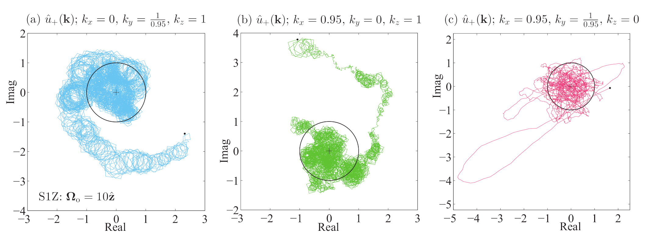
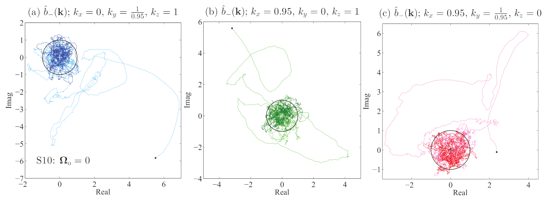
We have already seen how well the prediction (84) works by considering Figure 1 and Figure 2, as well as Table 1 and Table 2, as discussed in Section 3. To see the efficacy of (81), consider Figure 3, while, for (82) and (83), consider Figure 4 and Figure 5, respectively. Please note that Figure 3c represents the general behavior originally expected of all coefficients [19,20], i.e., that of a zero-mean random variable. Figure 1 and Figure 2 demonstrate that this expected ergodicity is clearly broken, while Figure 3, Figure 4 and Figure 5 show that expected behavior may be slow in occurring.

9. The Internal Dipole Magnetic Field

9.1. Periodic Box

Let us define the magnetic field associated with the $n=4$ and $\mathbf{k}=\underline{\mathbf{k}}$ Fourier modes as ${\mathbf{b}}_d\left(\mathbf{x}\right)$ (d for ‘dipole’) and the remainder as $\mathbf{h}\left(\mathbf{x}\right)$, where

$${\mathbf{b}}_d\left(\mathbf{x}\right)=N^{-3/2}\sum _{\underline{\mathbf{k}}}{\tilde{b}}_{+}\left(\underline{\mathbf{k}}\right)exp(i\underline{\mathbf{k}}·\mathbf{x}),\mathbf{h}\left(\mathbf{x}\right)=\mathbf{b}\left(\mathbf{x}\right)-{\mathbf{b}}_d\left(\mathbf{x}\right).$$

(85)

Note that ${\mathbf{j}}_d\left(\mathbf{x}\right)=\nabla \times {\mathbf{b}}_d\left(\mathbf{x}\right)={\mathbf{b}}_d\left(\mathbf{x}\right)$.

The expected energy contained in ${\mathbf{b}}_d\left(\mathbf{x}\right)$ is $〈E_M^d〉$ and in the remainder $\mathbf{h}\left(\mathbf{x}\right)$ is $〈E_M^h〉=〈E_M-E_M^d〉$, while (72) gives us $〈E_K〉$, to leading order:

$$\begin{array}{ccc}& & 〈E_M^d〉=\frac{1}{N^3}\sum _{{\underline{\mathbf{k}}}^{\prime }}|{\tilde{b}}_{+}\left(\underline{\mathbf{k}}\right){|}^2=\underline{k}\left|〈H_M〉\right|,\hfill \\ \hfill \end{array}$$

(86)

$$\begin{array}{ccc}& & 〈E_M^h〉=〈E_K〉=\frac{1}{2}\left(\mathcal{E}-\underline{k}\left|{\mathcal{H}}_M\right|\right).\hfill \end{array}$$

(87)

(Again, the sum over ${\underline{\mathbf{k}}}^{\prime }$ means that only independent modes $\underline{\mathbf{k}}$ are included). These may be considered ‘thermodynamic relations’ for ideal, rotating MHD turbulence. Note that (86) above, in conjunction with (44) implies that, again to leading order,

$$|〈H_M〉|=\frac{1}{N^3}\sum _{{\underline{\mathbf{k}}}^{\prime }}\frac{|{\tilde{b}}_{+}\left(\underline{\mathbf{k}}\right){|}^2}{\underline{k}}.$$

(88)

Thus, essentially all of the contribution to $|{\mathcal{H}}_M|$ comes from the ${\tilde{b}}_{+}\left(\underline{\mathbf{k}}\right)$. In the periodic box, which is a 3-torus, the magnetic field is completely internal, since there is no external volume, topologically speaking.

9.2. Spherical Shell

In the spherical shell case, however, there is an external volume and the spherical analogue of (88) allows us to relate the external dipole field to the internal poloidal field and therefore finally to know something about the internal, toroidal part of the Earth’s magnetic field. In the spherical shell model of [7], which uses homogeneous b.c.s, the statistical mechanics of the ideal magneto-fluid is essentially identical to that of the Fourier periodic box case. The only differences are superficial, in that indexing by the components of $\mathbf{k}$ is replaced by indexing with degree l and order m of the spherical harmonic $Y_{lm}(\theta ,\phi )$ and the number n of the zero $k_{ln}$ of the radial functions ${\widehat{g}}_l\left(k_{ln}r\right)$ at $r=1$; in the non-dimensional model, $r=1$ corresponds to the inner core radius $R_{IC}=1220$ km. (In dealing with an ellipsoidal shell, the order m of $Y_{lm}(\theta ,\phi )$ is also needed as $k_{ln}\to k_{lmn}$ [9]. Here, we focus only on a spherically symmetric shell.)

In a rotating spherical shell, MHD turbulence has energy E (where $E=E_K+E_M$) and magnetic helicity $H_M$ as ideal invariants, just as in the rotating periodic box. Thus, $〈E〉=\mathcal{E}$ and $〈H_M〉={\mathcal{H}}_M$, where $\mathcal{E}$ and ${\mathcal{H}}_M$ are constants. In [7], the expressions for $E_M$ and $H_M$ are given as

$$\begin{array}{ccc}\hfill E_M& =& \frac{1}{2}\sum _{l,m,n}\left(|b_{lmn}{|}^2+k_{ln}^2{\left|a_{lmn}\right|}^2\right),\hfill \\ \hfill \end{array}$$

(89)

$$\begin{array}{ccc}\hfill H_M& =& \sum _{l,m,n}{a}_{lmn}^{*}{b}_{lmn}.\hfill \end{array}$$

(90)

Above, the coefficients $a_{lmn}$ are associated with the poloidal part of the internal magnetic field and the coefficients $b_{lmn}$ are associated with the toroidal part of the internal magnetic field.

Traditional wisdom states that we cannot know the $b_{lmn}$. However, if we apply our periodic box results to the spherical shell, we see this belief may need revision. First, we recall that the smallest spherical shell dimensionless wavenumber for an Earth-like model is $\underline{k}=k_{11}=1.8638\dots$ (the next smallest wavenumber is $k_{21}=2.1497\dots$). The spherical shell version of (86) is

$${\mathcal{E}}_M^d=k_{11}\left|{\mathcal{H}}_M\right|.$$

(91)

Following (88), we expect that essentially all of the magnetic helicity will come from the dipole part of ${\mathcal{E}}_M$ and truncate the summations (89) and (90) to the $l=1$ and $n=1$ terms. Setting $|{\mathcal{H}}_M|=+{\mathcal{H}}_M$, for ${\mathcal{H}}_M>0$, we have

$$\sum _{m=-1}^1{〈b_{1m1}-k_{11}{a}_{1m1}〉}^2=0.$$

(92)

Thus, we know the dipole part of the toroidal magnetic field in terms of the poloidal field: $b_{1m1}=k_{11}{a}_{1m1}$. This leads us to make the estimates discussed earlier in Section 3.2 and which may be reviewed there.

10. Broken Ergodicity and Broken Symmetry

Here, we discuss the differences between the $k=\underline{k}$ eigenvariables ${\tilde{v}}_4\left(\underline{\mathbf{k}}\right)$ and all the other eigenvariables ${\tilde{v}}_n\left(\mathbf{k}\right)$ in regard to their dynamical behavior. It will be assumed that $q_x=q_y=q_z=1$ as differential oblateness is obviated by rotation and most planets and stars, do, in fact, rotate.

10.1. Broken Ergodicity

The expectation values (81)–(84) yield rms values $|{\tilde{v}}_n{\left(\mathbf{k}\right)|}_{rms}\equiv {〈|{\tilde{v}}_n{\left(\mathbf{k}\right)|}^2〉}^{\frac{1}{2}}$, so that

$$\begin{array}{ccc}\hfill \left(\mathrm{a}\right)& & \frac{|{\tilde{v}}_4\left(\underline{\mathbf{k}}\right){|}_{rms}}{N^{3/2}}={\left(\frac{\underline{k}\left|{\mathcal{H}}_M\right|}{3}\right)}^{1/2},n=4,k=1;\hfill \\ \hfill \\ \hfill \left(\mathrm{b}\right)& & \frac{|{\tilde{v}}_n{\left(\mathbf{k}\right)|}_{rms}}{N^{3/2}}\approx \frac{{\left(\mathcal{E}-\underline{k}\left|{\mathcal{H}}_M\right|\right)}^{1/2}}{2{\mathcal{M}}^{1/2}},\mathrm{all}\mathrm{others}.\hfill \end{array}$$

(93)

Again, from (74), ${\tilde{v}}_{1,2}\left(\mathbf{k}\right)={\tilde{u}}_{-,+}\left(\mathbf{k}\right)$ and ${\tilde{v}}_{3,4}\left(\mathbf{k}\right)={\tilde{b}}_{-,+}\left(\mathbf{k}\right)$. In (b), the expected magnitude is just the standard deviation because the associated mean of ${\tilde{v}}_n\left(\mathbf{k}\right)$ may be taken as zero. In (a), however, the expected magnitude may represent the magnitude of the mean of ${\tilde{b}}_{+}\left(\underline{\mathbf{k}}\right)$, rather than its standard deviation, for the following reasons.

Consider the modal dynamic Equations (30) with $\nu =0$ and (31) with $\eta =0$. Furthermore, in (30), because ${\mathbf{j}}_d\left(\mathbf{x}\right)\times {\mathbf{b}}_d\left(\mathbf{x}\right)=0$, we have $\tilde{\mathbf{S}}({\mathbf{j}}_d,{\mathbf{b}}_d;\mathbf{k})=0$ and can then use (85) to write

$$\tilde{\mathbf{S}}(\mathbf{j},\mathbf{b};\mathbf{k})=\tilde{\mathbf{S}}({\mathbf{j}}_d,{\mathbf{b}}_h;\mathbf{k})+\tilde{\mathbf{S}}({\mathbf{j}}_h,{\mathbf{b}}_d;\mathbf{k})+\tilde{\mathbf{S}}({\mathbf{j}}_h,{\mathbf{b}}_h;\mathbf{k})$$

(94)

Using (93a,b) as size estimates, we see that the rms values of the first two terms on the right are ∼${\mathcal{M}}^{1/2}$ larger than the third term $\tilde{\mathbf{S}}({\mathbf{j}}_h,{\mathbf{b}}_h;\mathbf{k})$, which is the same size as $\tilde{\mathbf{S}}(\mathbf{u},\mathbf{\omega };\mathbf{k})$ in (30).

In (31), $\tilde{\mathbf{S}}(\mathbf{u},\mathbf{b};\mathbf{k})$ can be written as

$$\tilde{\mathbf{S}}(\mathbf{u},\mathbf{b};\mathbf{k})=\tilde{\mathbf{S}}(\mathbf{u},{\mathbf{b}}_d;\mathbf{k})+\tilde{\mathbf{S}}(\mathbf{u},{\mathbf{b}}_h;\mathbf{k})$$

(95)

Again using (93a,b), we also see that the rms value of the first term on the right is ∼${\mathcal{M}}^{1/2}$ larger than the second term.

Using these estimates, estimate the rms sizes of the right sides of (30) and (31) as

$$\frac{|\tilde{\mathbf{S}}{(\mathbf{j},\mathbf{b};\mathbf{k})|}_{rms}}{N^{3/2}}\sim \frac{|\tilde{\mathbf{S}}{(\mathbf{u},\mathbf{b};\mathbf{k})|}_{rms}}{N^{3/2}}\sim \frac{1}{{\mathcal{M}}^{1/2}}.$$

(96)

From these and (93), we get

$$\begin{array}{ccc}& & \frac{dln|{\tilde{v}}_4(\underline{\mathbf{k}},t){|}_{rms}}{dt}\sim \frac{1}{{\mathcal{M}}^{1/2}},k=1,n=4,\hfill \\ \hfill \end{array}$$

(97)

$$\begin{array}{ccc}& & \frac{dln|{\tilde{v}}_n{(\mathbf{k},t)|}_{rms}}{dt}\sim 1,\mathrm{all}\mathrm{others}.\hfill \end{array}$$

(98)

What this implies dynamically is that, in equilibrium, the ‘dipole’ eigenvariables ${\tilde{v}}_4(\underline{\mathbf{k}},t)={\tilde{b}}_{+}(\underline{\mathbf{k}},t)$, which may be large, have, on average, fluctuations in magnitude comparable in size to the other ${\tilde{v}}_n(\mathbf{k},t)$, which are all very small. In particular, the fluctuations of these other ${\tilde{v}}_n(\mathbf{k},t)$ are of the same size as their rms magnitudes and so they behave like zero-mean random variables, as expected. However, the rms values of one or more of the ${\tilde{b}}_{+}(\underline{\mathbf{k}},t)$ are so large compared to their fluctuations that they exhibit nonergodic behavior, i.e., they have relatively large mean values over very long times, i.e., the exhibit ‘broken ergodicity.’ This phenomenon will be made clearer in the next subsection, where we also discuss ‘broken symmetry.’

10.2. Broken Symmetry

We have seen that, dynamically, the magnitudes of a ‘dipole’ eigenvariable ${\tilde{v}}_4(\underline{\mathbf{k}},t)={\tilde{b}}_{+}(\underline{\mathbf{k}},t)$, once large enough, can become effectively constant over a long time because its fluctuation in magnitude are very small. Often, one of the ${\tilde{b}}_{+}(\underline{\mathbf{k}},t)$, for $\underline{\mathbf{k}}=\underline{\mathbf{x}}$, $\underline{\mathbf{y}}$ or $\underline{\mathbf{z}}$ does not become as large as predicted by (83). These predictions are just average values over the ensemble and to see what is really going on we must consider the sum of the expectation values (86). As in Section 10.1, we will use $q_x=q_y=q_z=0$ so that $\underline{k}=1$ and $\underline{\mathbf{k}}=\widehat{\mathbf{x}}$, $\widehat{\mathbf{y}}$ or $\widehat{\mathbf{z}}$. What (83) implies is that the six components of the three ${\tilde{b}}_{+}(\underline{\mathbf{k}},t)$ define a six component vector in a 6D real space or a three component vector in a complex 3D space; for compactness, we define a vector ${\tilde{\mathsf{v}}}_d$ and dot product $|{\tilde{\mathsf{v}}}_d{|}^2={\tilde{\mathsf{v}}}_d^{†}{\tilde{\mathsf{v}}}_d$ in a 3D complex space:

$${\tilde{\mathsf{v}}}_d=\frac{1}{N^{3/2}}\left[\begin{array}{c}{\tilde{b}}_{+}\left(\widehat{\mathbf{x}}\right)\\ {\tilde{b}}_{+}\left(\widehat{\mathbf{y}}\right)\\ {\tilde{b}}_{+}\left(\widehat{\mathbf{z}}\right)\end{array}\right],|{\tilde{\mathsf{v}}}_d{|}^2=\left|{\mathcal{H}}_M\right|.$$

(99)

The endpoint of ${\tilde{\mathsf{v}}}_d$ is a quasi-stationary point on the surface of the hypersphere of radius $\sqrt{|{\mathcal{H}}_M|}$ in a 6D subspace of the $8\mathcal{M}$-D phase space $\mathsf{\Gamma }$. The coordinates of the 6D space can undergo an arbitrary orthogonal rotation (or a unitary transformation in the complex 3D space) that puts the point of the vector on any desired point on the surface. Thus, although (93a) predicts that all ${\tilde{b}}_{+}(\underline{\mathbf{k}},t)$ will have the same magnitude, this does not take into account that a suitable orthogonal transformation of initial conditions in the whole phase space will lead to the evolution of ${\tilde{\mathsf{v}}}_d$ pointing in any direction its 6D space that we choose, at least for the non-rotating case.

The fact that ${\tilde{\mathsf{v}}}_d$ will exhibit broken ergodicity (i.e., it becomes quasi-stationary while undergoing only small fluctuations. However, initial conditions will also impose a particular direction on it, leading to a broken symmetry amongst the ${\tilde{b}}_{+}(\underline{\mathbf{k}},t)$ with regard to the expectation values (83). The phenomenon of broken symmetry has been noted before [23,43], as we have also noted many times the appearance of broken ergodicity [6,22,23,39]. Here, we see how these aspects of MHD turbulence are connected.

In equilibrium, the magnitudes of the ${\tilde{b}}_{+}(\underline{\mathbf{k}},t)$, for $\underline{\mathbf{k}}=\underline{\mathbf{x}}$, $\underline{\mathbf{y}}$, and $\underline{\mathbf{z}}$ are often not that different in the non-rotating ideal case but may vary appreciably, as Figure 1a shows. However, when rotation is imposed in the ideal case, the eigenfunction ${\tilde{b}}_{+}(\underline{\mathbf{k}},t)$ with $\underline{\mathbf{k}}$ parallel to ${\mathsf{\Omega }}_{\mathrm{o}}$ has essentially all the dipole energy (regardless of the values of the $q_j$), as Figure 2b–d demonstrate. In the real case of forced, dissipative MHD turbulence, this phenomenon is also usually observed numerically, although some forcing mechanism may disrupt this process, as seen in Figure 7 of Reference [9].

However, alignment with the rotation axis seems fairly ubiquitous in numerical simulations, as well as in planets and stars. We will now discuss possible reasons for this ‘dipole alignment’.

11. Dipole Alignment

One of the mysteries of magnetism is just how the dipole moment of the Earth and other planets align themselves with their rotation axis. Ref. [44] proposed that magnetic moment and angular momentum were directly proportional, though this conjecture has not held up to scrutiny; here we have shown that the magnetic moment is essentially proportional to $\sqrt{|{\mathcal{H}}_M|}$. [9] suggested that a difference in the ellipticities of the Earth’s inner and outer cores could lead to alignment if the smallest wavenumber was along the rotation axis.

11.1. Differential Oblateness Effects

To test the hypothesis that differential oblateness was important with a Fourier method code, wavevector components were adjusted, as detailed in Section 4.2, to $k_j\to q_j{k}_j$ and x-space position components to $x_j\to x_j/q_j$, $j=x,y,z$, with $q_x{q}_y{q}_z=1$. This adjustment insured that $\mathbf{k}·\mathbf{x}$ was invariant, so that the Fourier transforms (13) and (14), as well as the numerical transform method, were unaffected. When the grids were stretched with ${\mathsf{\Omega }}_{\mathrm{o}}=0$, the coefficients with the smallest wavenumber noticeably increased in magnitude compared to their unstretched values, as Figure 1 shows. However, the effect of differential oblateness was completely overshadowed when rotation ${\mathsf{\Omega }}_{\mathrm{o}}\ne 0$ was introduced, as is shown in Figure 2. The oblateness of the inner and outer cores is two orders of magnitude smaller than that modeled in our runs, so, for purposes of understanding the cause of dipole alignment, we need only use $q_x=q_y=q_z=1$ in the Fourier case, and keep the spherical shell model of [7] spherical.

11.2. Dynamical Effects

We know that the vector ${\tilde{\mathsf{v}}}_d$, whose three complex components are the ${\tilde{b}}_{+}\left(\widehat{\mathbf{k}}\right)$, where $\widehat{\mathbf{k}}=\widehat{\mathbf{x}},\widehat{\mathbf{y}},\widehat{\mathbf{z}}$, and is defined in (99), has almost constant magnitude $\sqrt{q_{min}\left|{\mathcal{H}}_M\right|}$. In the Fourier model, $q_{min}=1$ and in the spherical shell model, $q_{min}=1.8638$. Here, we work with the Fourier model. If we look at (31) and retain only those terms that contain one of the ${\tilde{b}}_{+}(\pm \widehat{\mathbf{k}})$, we get

$$\begin{array}{ccc}\hfill \frac{\mathrm{d}{\tilde{b}}_{+}\left(\widehat{\mathbf{x}}\right)}{\mathrm{d}t}& =& \frac{i}{N^{3/2}}\widehat{\mathbf{x}}\times \sum _{\widehat{\mathbf{k}}=\pm \widehat{\mathbf{y}}}^{\pm \widehat{\mathbf{z}}}\left[\tilde{\mathbf{u}}(\widehat{\mathbf{x}}-\widehat{\mathbf{k}})\times {\tilde{\mathbf{b}}}_{+}\left(\widehat{\mathbf{k}}\right)\right],\hfill \\ \hfill \end{array}$$

(100)

$$\begin{array}{ccc}\hfill \frac{\mathrm{d}{\tilde{b}}_{+}\left(\widehat{\mathbf{y}}\right)}{\mathrm{d}t}& =& \frac{i}{N^{3/2}}\widehat{\mathbf{y}}\times \sum _{\widehat{\mathbf{k}}=\pm \widehat{\mathbf{z}}}^{\pm \widehat{\mathbf{x}}}\left[\tilde{\mathbf{u}}(\widehat{\mathbf{y}}-\widehat{\mathbf{k}})\times {\tilde{\mathbf{b}}}_{+}\left(\widehat{\mathbf{k}}\right)\right],\hfill \\ \hfill \end{array}$$

(101)

$$\begin{array}{ccc}\hfill \frac{\mathrm{d}{\tilde{b}}_{+}\left(\widehat{\mathbf{z}}\right)}{\mathrm{d}t}& =& \frac{i}{N^{3/2}}\widehat{\mathbf{z}}\times \sum _{\widehat{\mathbf{k}}=\pm \widehat{\mathbf{x}}}^{\pm \widehat{\mathbf{y}}}\left[\tilde{\mathbf{u}}(\widehat{\mathbf{z}}-\widehat{\mathbf{k}})\times {\tilde{\mathbf{b}}}_{+}\left(\widehat{\mathbf{k}}\right)\right].\hfill \end{array}$$

(102)

Now, (21) and (33) tell us that

$$\begin{array}{ccc}\hfill \tilde{\mathbf{u}}(\mathbf{k},t)& =& {\overline{u}}_{+}(\mathbf{k},t)exp\left(i{\mathsf{\Omega }}_{\mathbf{k}}t\right){\widehat{\mathbf{e}}}_{+}\left(\mathbf{k}\right)+{\overline{u}}_{-}(\mathbf{k},t)exp(-i{\mathsf{\Omega }}_{\mathbf{k}}t){\widehat{\mathbf{e}}}_{-}\left(\mathbf{k}\right).\hfill \end{array}$$

(103)

Therefore, for ${\mathsf{\Omega }}_{\mathrm{o}}={\mathsf{\Omega }}_{\mathrm{o}}\widehat{\mathbf{z}}$, on the right sides of the equations given above, all of the terms containing $\tilde{\mathbf{u}}(\widehat{\mathbf{z}}\pm \widehat{\mathbf{x}})$ or $\tilde{\mathbf{u}}(\widehat{\mathbf{z}}\pm \widehat{\mathbf{y}})$ or their complex conjugates have oscillations with angular frequencies $\pm {\mathsf{\Omega }}_{\mathbf{k}}=\pm \sqrt{2}{\mathsf{\Omega }}_{\mathrm{o}}$. If we watch the dynamical system over a time $T>>\sqrt{2}\pi /{\mathsf{\Omega }}_{\mathrm{o}}$, then we may expect these terms to average out to zero. In that case, (100)–(102) become

$$\begin{array}{ccc}\hfill \frac{\mathrm{d}{\tilde{b}}_{+}\left(\widehat{\mathbf{x}}\right)}{\mathrm{d}t}& \approx & \frac{i}{N^{3/2}}\widehat{\mathbf{x}}\times \sum _{\widehat{\mathbf{k}}=\pm \widehat{\mathbf{y}}}\left[\tilde{\mathbf{u}}(\widehat{\mathbf{x}}-\widehat{\mathbf{k}})\times {\tilde{\mathbf{b}}}_{+}\left(\widehat{\mathbf{k}}\right)\right],\hfill \\ \hfill \end{array}$$

(104)

$$\begin{array}{ccc}\hfill \frac{\mathrm{d}{\tilde{b}}_{+}\left(\widehat{\mathbf{y}}\right)}{\mathrm{d}t}& \approx & \frac{i}{N^{3/2}}\widehat{\mathbf{y}}\times \sum _{\widehat{\mathbf{k}}=\pm \widehat{\mathbf{x}}}\left[\tilde{\mathbf{u}}(\widehat{\mathbf{y}}-\widehat{\mathbf{k}})\times {\tilde{\mathbf{b}}}_{+}\left(\widehat{\mathbf{k}}\right)\right],\hfill \\ \hfill \end{array}$$

(105)

$$\begin{array}{ccc}\hfill \frac{\mathrm{d}{\tilde{b}}_{+}\left(\widehat{\mathbf{z}}\right)}{\mathrm{d}t}& \approx & 0.\hfill \end{array}$$

(106)

The expression (106) is true once ${\tilde{b}}_{+}\left(\widehat{\mathbf{z}}\right)$ grows to be very large, while (104) and (105) tell us that ${\tilde{b}}_{+}\left(\widehat{\mathbf{x}}\right)$ and ${\tilde{b}}_{+}\left(\widehat{\mathbf{y}}\right)$ are still subject to fluctuations (again, we assume ${\mathsf{\Omega }}_{\mathrm{o}}={\mathsf{\Omega }}_{\mathrm{o}}\widehat{\mathbf{z}}$). Presumably, ${\tilde{b}}_{+}\left(\widehat{\mathbf{x}}\right)$ and ${\tilde{b}}_{+}\left(\widehat{\mathbf{y}}\right)$ ‘regress to the mean,’ which is zero because they are subject to relatively large fluctuations, while ${\tilde{b}}_{+}\left(\widehat{\mathbf{z}}\right)$ has relatively insignificant fluctuations to drive it from dominance. Further analysis is beyond the scope of this paper and may require a deeper mathematical analysis along the lines of [45].

12. Conclusions

Here, we have presented theoretical and computational results in magnetohydrodynamic turbulence that we feel are essential to understanding the geodynamo. Again, these results are based on a mathematical model that focuses on MHD turbulence, but ignores compressibility and thermal effects, as well as imposing model-dependent boundary conditions. Our conclusions are: (1) In the Earth’s outer core, the energy of the magnetic dipole is equal to the magnetic helicity multiplied by the dipole wavenumber. (2) The connection between magnetic helicity and dipole field in the Earth’s liquid core gives us the toroidal part of the internal dipole field. (3) Knowing this allows the estimate the mean internal dipole field strength is 3 mT. (4) Differential oblateness can cause dipole alignment, but rotation appears to be far more important. (5) Dipole alignment appears related to hydrodynamic inertial waves, but exactly how is still an open question.

References

- Larmor, J. How Could a Rotating Body Such as the Sun Become a Magnet? Report British of the Association for the Advancenment of Science; John Murray: London, UK, 1919; pp. 159–160. [Google Scholar]
- Glatzmaier, G.A.; Roberts, P.H. A three-dimensional self-consistent computer simulation of a geomagnetic field reversal. Nature 1995, 377, 203–209. [Google Scholar] [CrossRef]
- Glatzmaier, G.A.; Roberts, P.H. A three-dimensional convective dynamo solution with rotating and finitely conducting inner core and mantle. Phys. Earth Planet. Int. 1995, 91, 63–75. [Google Scholar] [CrossRef]
- Kuang, W.; Bloxham, J. An Earth-like numerical dynamo model. Nature 1997, 389, 371–374. [Google Scholar] [CrossRef]
- Davidson, P.A. Turbulence in Rotating and Electrically Conducting Fluids; Cambridge University Press: Cambridge, UK, 2013; p. 532. [Google Scholar]
- Shebalin, J.V. Broken ergodicity in magnetohydrodynamic turbulence. Geophys. Astrophys. Fluid Dyn. 2013, 107, 411–466. [Google Scholar] [CrossRef]
- Shebalin, J.V. Broken ergodicity, magnetic helicity, and the MHD dynamo. Geophys. Astrophys. Fluid Dyn. 2013, 107, 353–375. [Google Scholar] [CrossRef]
- Shebalin, J.V. Dynamo action in dissipative, forced, rotating MHD turbulence. Phys. Plasmas 2016, 23, 062318. [Google Scholar] [CrossRef]
- Shebalin, J.V. Magnetohydrodynamic turbulence and the geodynamo. Phys. Earth Planet. Inter. 2018, 285, 59–75. [Google Scholar] [CrossRef]
- Hughes, D.W. Mean field electrodynamics: Triumphs and tribulations. J. Plasma Phys. 2018, 84, 735840407. [Google Scholar] [CrossRef]
- Shebalin, J.V. Magnetic Helicity and the Solar Dynamo. Entropy 2019, 21, 811. [Google Scholar] [CrossRef]
- Teissier, J.-M.; Müller, W.-C. In verse transfer of magnetic helicity in supersonic magnetohydrodynamic turbulence. J. Phys. Conf. Ser. 2020, 1623, 012011. [Google Scholar] [CrossRef]
- Orszag, S.A.; Patterson, G.S. Numerical simulation of three-dimensional homogeneous isotropic turbulence. Phys. Rev. Lett. 1972, 28, 76–79. [Google Scholar] [CrossRef]
- Gazdag, J. Time-differencing schemes and transform methods. J. Comp. Phys. 1976, 20, 196–207. [Google Scholar] [CrossRef]
- Chandrasekhar, S.; Kendall, P.C. On Force-Free Magnetic Fields. Astrophys. J. 1957, 12, 457–460. [Google Scholar] [CrossRef]
- Morrish, J.S.; Moon, W.M. Velocity field and thickness of a laminar boundary layer at the core-mantle boundary. J. Geophys. Res. 1991, 96, 14569–14575. [Google Scholar] [CrossRef]
- Thébault, E.; Finlay, C.C.; Beggan, C.D.; Alken, P.; Aubert, J.; Barrois, O.; Bertrand, F.; Bondar, T.; Boness, A.; Brocco, L.; et al. International Geomagnetic Reference Field: The 12th generation. Earth Planets Space 2015, 67, 79. [Google Scholar] [CrossRef]
- Buffett, B.A. Tidal dissipation and the strength of the Earth’s internal magnetic field. Nature 2000, 468, 952–955. [Google Scholar] [CrossRef]
- Frisch, U.; Pouquet, A.; Leorat, J.; Mazure, A. Possibility of an inverse cascade of magnetic helicity in magnetohydrodynamic turbulence. J. Fluid Mech. 1975, 68, 769–778. [Google Scholar] [CrossRef]
- Lee, T.D. On some statistical properties of Hydrodynamical and magneto-hydrodynamical fields. Q. Appl. Math. 1952, 10, 69–74. [Google Scholar] [CrossRef]
- Palmer, R.G. Broken ergodicity. Adv. Phys. 1982, 31, 669–735. [Google Scholar] [CrossRef]
- Shebalin, J.V. Anisotropy in MHD Turbulence Due to a Mean Magnetic Field. Ph.D. Thesis, College of William and Mary, Williamsburg, VA, USA, 1982. [Google Scholar]
- Shebalin, J.V. Broken symmetry in ideal magnetohydrodynamic turbulence. Phys. Plasmas 1994, 1, 541–547. [Google Scholar] [CrossRef][Green Version]
- Bardsley, O.P.; Davidson, P.A. Inertial-Alfven waves as columnar helices in planetary cores. J. Fluid Mech. 2016, 805, R2. [Google Scholar] [CrossRef]
- Ranjan, A.; Davidson, P.A. Columnar heat transport via advection induced by inertial waves. Int. J. Heat Fluid Flow 2021, 87, 108703. [Google Scholar] [CrossRef]
- Soward, A.M. The Earth’s Dynamo. Geophys. Astrophys. Fluid Dyn. 1991, 62, 191–209. [Google Scholar] [CrossRef]
- Biskamp, D. Magnetohydrodynamic Turbulence; Cambridge University Press: Cambridge, UK, 2003; Chapter 2. [Google Scholar]
- Patterson, G.S.; Orszag, S.A. Spectral calculation of isotropic turbulence: Efficient removal of aliasing interaction. Phys. Fluids 1971, 14, 2538–2541. [Google Scholar] [CrossRef]
- Favier, B.F.N.; Godeferd, F.S.; Cambon, C. On the effect of rotation on magnetohydrodynamic turbulence at high magnetic Reynolds number. Geophys. Astrophys. Fluid Dyn. 2012, 106, 89–111. [Google Scholar] [CrossRef][Green Version]
- Shebalin, J.V. Plasma relaxation and the turbulent dynamo. Phys. Plasmas 2009, 16, 072301. [Google Scholar] [CrossRef]
- Mininni, P.D.; Montgomery, D. Magnetohydrodynamic activity inside a sphere. Phys. Fluids 2006, 18, 116602. [Google Scholar] [CrossRef]
- Mininni, P.D.; Montgomery, D.; Turner, L. Magnetohydrodynamic activity inside a sphere. New J. Phys. 2007, 9, 303–330. [Google Scholar] [CrossRef]
- Shebalin, J.V. Ideal homogeneous magnetohydrodynamic turbulence in the presence of rotation and a mean magnetic field. J. Plasma Phys. 2006, 72, 507–524. [Google Scholar] [CrossRef]
- Elsässer, W.M. Hydromagnetic dynamo theory. Rev. Mod. Phys. 1956, 28, 135–163. [Google Scholar] [CrossRef]
- Woltjer, L. A theorem on force-free magnetic fields. Proc. Natl. Acad. Sci. USA 1958, 44, 489–491. [Google Scholar] [CrossRef] [PubMed]
- Shebalin, J.V. Global invariants in ideal magnetohydrodynamic turbulence. Phys. Plasmas 2013, 20, 102305. [Google Scholar] [CrossRef]
- Kraichnan, R.H. Helical turbulence and absolute equilibrium. J. Fluid Mech. 1973, 59, 745–752. [Google Scholar] [CrossRef]
- Fyfe, D.; Montgomery, D. High beta turbulence in two-dimensional magneto-hydrodynamics. J. Plasma Phys. 1976, 16, 181–191. [Google Scholar] [CrossRef]
- Shebalin, J.V. Broken ergodicity and coherent structure in homogeneous turbulence. Physica D 1989, 37, 173–191. [Google Scholar] [CrossRef]
- Silvester, J.R. Determinants of block matrices. Math. Gaz. 2000, 84, 460–467. [Google Scholar] [CrossRef]
- Shebalin, J.V. The homogeneous turbulent dynamo. Phys. Plasmas 2008, 15, 022305. [Google Scholar] [CrossRef]
- Khinchin, A.I. Mathematical Foundations of Statistical Mechanics; Dover: New York, NY, USA, 1949; pp. 137–145. [Google Scholar]
- Shebalin, J.V. Broken symmetries and magnetic dynamos. Phys. Plasmas 2007, 14, 102301. [Google Scholar] [CrossRef]
- Blackett, P.M.S., XI. The magnetic field of massive rotating bodies, London, Edinburgh, and Dublin. Phil. Mag. J. Sci. 1949, 40, 125–150. [Google Scholar] [CrossRef]
- Cheng, B.; Mahalov, A. General results on zonation in rotating systems with a β-effect and the electromagnetic force. In Zonal Jets: Phenomenology, Genesis, and Physics; Galperin, B., Read, P.L., Eds.; Cambridge University Press: Cambridge, UK, 2019; pp. 209–219. [Google Scholar]
Figure 1.
Wavenumber , positive helicity magnetic variables, normalized: , for runs (a) C0, (b) S10, (c) S20, (d) S30 of Table 1. These trajectories all began close to the origin. The behavior of the , in these graphs illustrates the influence of initial conditions and the presence of broken symmetry, e.g., in (a), where all the , the expectation that all of the have the same magnitudes, which is represented by the dashed circular arc, is not met.
Figure 2.
Wavenumber , positive helicity magnetic variables, normalized: , for runs (a) S10, (b) S1X, (c) S1Y, (d) S1Z of Table 1. Comparing these figures with those in Figure 1, it is clear that rotation is more important than oblation (at least for the large value ).
Figure 3.
Wavenumber , positive helicity kinetic variables, normalized: , for run S3Z of Table 1. The factor removes the cyclic behavior of inertial waves; see Equation (33). The unit circles indicate , i.e., the expected variance of unity. Initial values () of these trajectories are marked with a •. These graphs indicate that the non-dipole variables behave as expected.
Figure 4.
Run S10: wavenumber , negative helicity magnetic variables, normalized: . Initial values () of these trajectories are marked with a • and the darker part of the trajectory shows the last half of the run. The unit circles indicate , i.e., the expected variance of unity. These graphs indicate that the non-dipole variables behave as expected. In fact, all coefficients were expected to be ergodic, well-behaved zero-mean variables; however, consider Figure 1 and Figure 2, which show that ergodicity is strongly broken for some of the lowest wavenumber coefficients.
Figure 5.
Run S1X: wavenumber , negative helicity magnetic variables, normalized: , for run S1X of Table 1. Initial () points are marked with a • and the darker part of the trajectory shows the last half of the run. The unit circles indicate , i.e., the expected variance of unity. These graphs show that the non-dipole variables are tending to expected behavior, though rotation slows the process down, compared to Figure 4.