1. Introduction
Turbulence in the context of fluid dynamics often refers to the
chaotic nature of fluid motion in terms of velocity and pressure. This kind of definition suggests deterministic chaotic and turbulent characteristics [
1], which must be distinguished from random behaviour. However, also for deterministic turbulent flows, some statistical laws apply in the same manner as for linear systems [
2], whereas their statistics may widely differ; they usually are of Lévy-type and show long tail distributions that are produced by rare large-scale fluctuations and clustering phenomena of anomalous eddy diffusion. However, different than for random systems in phase space, for example, turbulent ones may exhibit highly ordered structures, called strange attractors [
1], which relate to nonlinear, nonloca,l and fractional features of turbulence [
3]. Additionally, nonequilibrium [
4], nonextensive [
5], and universal behaviour [
6] characterize turbulent flows. In this article, we focus on universality, and, by this, we mean the independence of statistical properties of small-scale eddies from the overall nature of the fluid (forcing of the fluid, geometry, and size of the basin, etc.). One of the first illustrations of this universal character dates back to 1941, when the Kolmogorov theory emerged. The latter states that, regardless of a fluid’s properties, the turbulent flow exhibits a scale-invariant structure at the inertial region. Based on this finding, Kolmogorov was able to characterize this zone as a power law of the energy spectrum with an exponent that is equal to
[
7], which for flows of Reynolds numbers smaller than infinity, is modified by an intermittency correction [
8,
9].
Subsequently, many areas of turbulence research were driven by the fundamental challenge of identifying generalizable turbulence properties and turbulent flow similarities with the aim of investigating and defining turbulent flow universal patterns [
10]. In particular, because fluid mixing is mainly driven by the smallest diffusive scales, many studies have been devoted to the assessment of the fundamental and intrinsic topological aspects of these flow scales. In this regard, the pure kinematic approach provides a general and useful tool to describe the small scales of fluid motions. One of these quantities, which is often of significant interest, is the velocity gradient tensor (VGT),
, which can be split into the sum of the strain-rate tensor,
, and the rotation-rate,
tensor, i.e., (see also Ref. [
11])
For many decades, this decomposition has been an essential tool for the turbulence community [
12] due to the simplicity of its formulation and the physical insight that it provides. It has also led to the construction of various subgrid-scale models [
13,
14] and the development of flow visualization tools that are based on simulation realizations [
15]. However, recent studies have shown the importance of considering the contribution of shear in both the identification of vortex structure regions and strain rate [
15]. Indeed, vorticity cannot distinguish between pure shearing motion and vortical motion, and the strain rate cannot distinguish between straining motion and shearing motion. By considering two-dimensional DNS of a subsonic mixing layer behind a flat plate, [
16] showed the importance of shear regions in the identification of vortex structures. Most of the discussions on the structural aspects of turbulence adopt Eulerian vortex detection methods, like the
Q-criterion, the
-criterion, and its closely related swirling strength criterion (
-criterion [
17]), or the
-criterion [
18]. In all of these criteria, a scalar field, which is derived from the decomposition (
1) and/or eigenvalues of the VGT, is used as a “marker” to indicate whether a given point in the flow field belongs to a vortex or not [
19]. Therefore, vortices are identified as the connected regions that are mapped by such scalar fields. Recently, [
20] formulated a Liutex-based VGT (previously called Rortex) decomposition for locally fluid-rotational points (the VGT has complex eigenvalues) in a turbulent flow field. This method [
20] of separating the rigid-body-rotation “Liutex” from shear in vorticity is more computationally viable and it has been employed in some studies [
17] for the investigation of coherent vortex structures in turbulent flows. In another study, [
21] presented a decomposition of the VGT into normal and non-normal tensors, such that the non-normal counterpart represents the local effects of shear. Aside from these methods, [
15] originally introduced a robust triple decomposition method, from which a residual vorticity could be found to represent the pure rigid-body rotation of a fluid element. The cornerstone of this method is to decompose
as
where
,
and
denote normal-straining, pure-shearing, and rigid-body-rotation components of the VGT, respectively. According to [
15], the three components in Equation (
2) can be determined while using a suitable reference frame, called the
basic reference frame (BRF). The BRF refers to a special local coordinate system in which the effect of shear is maximal, so that the decomposition is unique.
Most of the studies that targeted this triple decomposition method (TDM) were carried out in two-dimensional configurations [
22,
23]. Under such flows, the identification of the basic reference can be analytically obtained and the extraction of the three motions is straightforward. Conversely, the analytical identification of the BRF is not possible in the general case where turbulence is comprised of three-dimensional fluid motions, and the extraction of vortices and internal shear layers are of considerable interest. In the general case, one can identify the BRF from a finite set of discrete frame representations by performing a series of discrete rotations of the reference frame [
15]. In this context, [
24] proposed a numerical procedure and then successfully applied it to the framework of three-dimensional incompressible homogeneous isotropic turbulence at Taylor Reynolds numbers,
and 140. One of the major findings of [
24] is that some of the strong shear regions, identified using the TDM and visualized as sheet-like structures, could not have been detected using the classical double decomposition. Indeed, TDM analysis characterizes these regions as high intensity shearing components, whereas, from the double decomposition, they appear as regions where the effects of the strain-rate tensor,
, and the rotation-rate tensor,
, are comparable. With this in mind, and given that only incompressible flows have been considered so far, we must question the accuracy of the TDM for more complex flows that are characterized by high turbulent Mach numbers,
. For instance, unlike the incompressible case, at high
, both the strong nonlinear coupling between the velocity and thermal fields and the occurrence of localized shocklets in the flow field lead to an additional and rapid conversion of the kinetic energy dissipation mechanism. The analysis of the flow topology in compressible flows has been investigated before; see, for example, the works of [
25,
26,
27,
28]. A general conclusion from these studies is that the appearances of the intense events tend to increase with
. These studies also indicate that, as
increases, strong compressions are more likely to occur than equally strong expansions.
The present work aims at extending the previous studies to the compressible high regime. Furthermore, we suggest a new numerical approach to determine the BRF with the aim of achieving high accuracy at a significantly reduced computational cost. We then apply the TDM and the new numerical procedure in order to define the BRF to a new DNS database of isotropic compressible turbulence with a turbulent Mach number ranging from (i.e., almost incompressible regime) to (i.e., highly compressible regime).
The remainder of this paper is organized, as follows.
Section 2 gives a brief overview of the governing equations with the methods and algorithms that were used in their numerical resolution.
Section 3 provides the general statistics of the generated DNS database. The invariants of the VGT are briefly recalled in
Section 4. Next, the methodology of
triple decomposition, as well as the procedure of determining the basic reference frame in
Section 5, are presented. By exploring its dependency on the turbulent Mach number, the VGT composition of a turbulent flow field is examined in detail in
Section 6. Finally,
Section 7 draws the key findings and conclusion of this analysis.
3. Dns Database
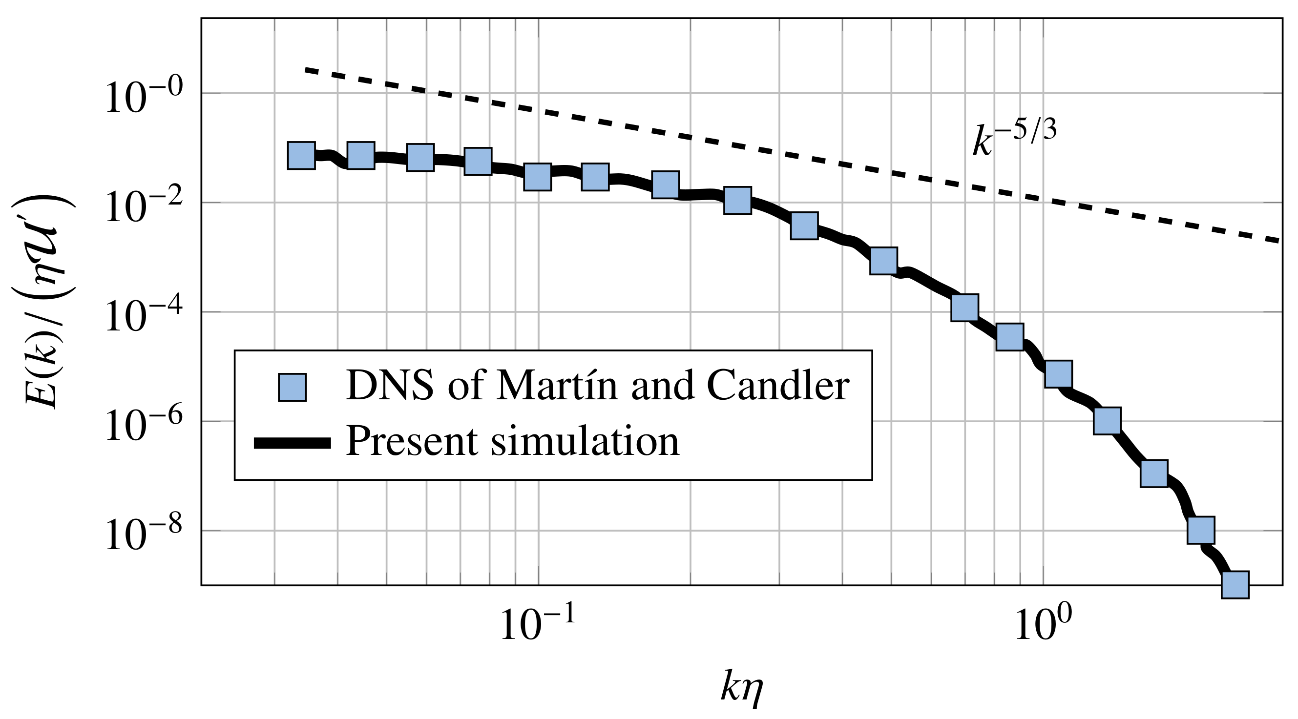
The decaying isotropic turbulence is an important model that is used to investigate the free compressible turbulence. In this context, ensuring that the turbulence is fully developed is important. Prior to the generation of the DNS database, the numerical procedure is first validated by comparing its result against the DNS data of [
34]. The validation test case consists of a decaying isotropic turbulence evolving in a three-dimensional periodic box with side length
that is uniformly discretized on 128 points per each coordinate direction. The velocity field is initialized by an isotropic state that is prescribed by the energy spectrum
where
k is the integer non-dimensional wave number and
is the most energetic wave number. A finite density, temperature, and dilatation fluctuations are also generated, as described by [
35]. The calculation is performed at a Reynolds number based on the longitudinal Taylor micro-scale
, where
and
, and at a turbulent Mach number
, where
a is the speed of sound. The initial flow-field is allowed to decay temporally for four dimensionless time units,
, where the time unit, herein, is the eddy turnover time that is defined as
. This choice allows for the energy spectrum
to develop an inertial range that decays as
. In
Figure 1, we depict the energy spectra in wave number space at
. These results show a very good agreement with the data of [
34]. Moreover, the energy spectrum is marginally consistent with a
scaling law in a smaller frequency range due to the limit of the spatial resolution in the present DNS (Note that a recently developed approach, based on the extraction of the rigid rotation part from the fluid motion (called Liutex-based vortex), allows following the −5/3 almost exactly over the whole range of frequencies [
10]).
Following this validation, the DNS database featuring six direct numerical simulations of temporal turbulence decay is conducted on a
point grid.
Table 1 summarizes the one-point statistics of the six simulated flows, obtained by freezing the temporal turbulence decay of periodic boxes, after approximately three eddy turnover times, which ensures that the turbulence is deemed to be developed and realistic. The turbulent Mach number,
, which is varied between
and
, is the main parameter of interest in this parametric study. The Taylor micro-scale Reynolds number,
, is considered to be common to all the cases and set almost to 100. The wave number
is selected to ensure that the fully developed homogeneous isotropic turbulence field has a broad range of length scales [
36].
The Kolmogorov length scale, which is defined from the kinetic energy dissipation rate per unit volume (
), is resolved on the retained grid discretization. Indeed, the resolution parameter
is in the range
, where
is the uniform grid spacing in each coordinate direction. This can be also verified in terms of the maximum resolved wave number in the grid (the half of the number of grid points in each direction). In the present DNS database,
finds its values in the range
. This range ensures that the small scales are well resolved in all of the database cases [
37]. In order to measure the onset of a realistic turbulence, the mean values of the velocity derivative skewness
and flatness
are used herein as criteria. These are defined, respectively, as
As it can be noticed from
Table 1, the magnitudes of both
and
increase with increasing
. This is a well-known feature that is due to the onset of shocklets in compressible turbulence [
38]. It is noteworthy to point out that, despite the comparability between the shock thickness and the grid length, as well as the fact that the shock thickness is not directly resolved by the
WENO-Z scheme, the total amount of dissipation across a shock is independent of numerical viscosity [
39]. Indeed, as shown by [
40], as long as the shocklet thickness is small, the total amount of dissipation across the shocks is independent of viscosity, and it depends only on the jump conditions across the shocks, which are preserved by the
WENO-Z scheme.
4. The Velocity Gradient Tensor and the Invariants of Its Characteristic Equation
The velocity-gradient tensor,
, is a
matrix that is given by
. The characteristic equation for
is
where
is the identity matrix and the first three invariants
P,
Q, and
R in Equation (
15) can be calculated as
where
and
are, respectively, the strain- and rotation-rate tensor components of
, defined as
As shown by [
41], the expression
P,
Q and
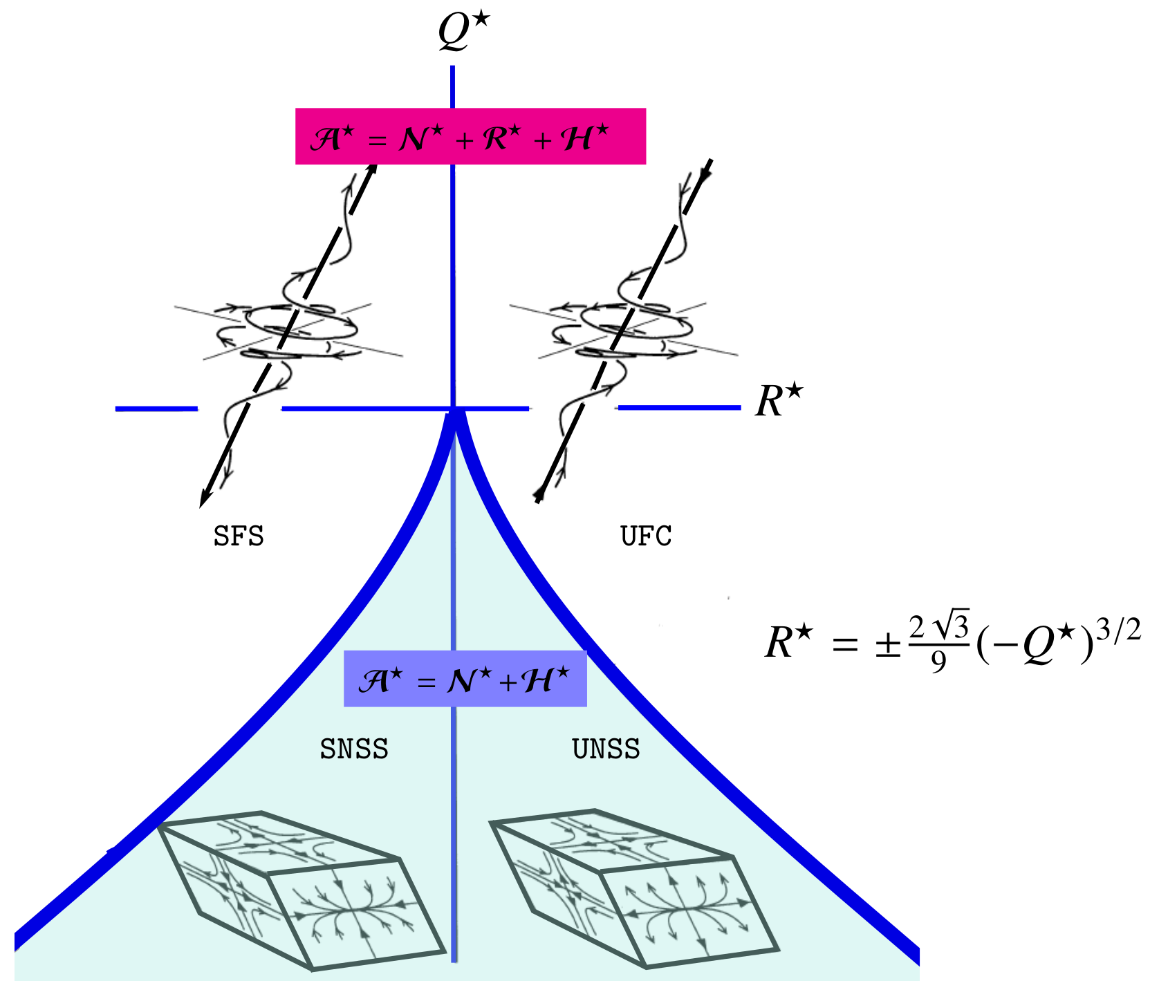
R is of a topological significance, because the
space is divided into several regions, and each region represents a particular flow topology. It is more convenient to analyze the flow topology in the
plane due to the spatial complexity of different zones present in the
space. To proceed, we reformulate the problem in terms of the anisotropic part of the deformation rate tensor, i.e.,
, where
denotes the divergence of the velocity. Therefore, we observe that, as in incompressible turbulence, by construction
. The use of the anisotropic tensor aims at (i) comparing the statistical properties of compressible turbulent structures and their dynamics with the incompressible case for which
and (ii) facilitating the discussions of local topological flow structures, since it reduces the space of comparison to the
plane [
26,
27]. All of the quantities computed from the anisotropic tensor are indicated with the superscript ⋆. In the new formulation, the second,
, and third invariants,
, are given by
These two invariants are of great importance from a topological point of view, because the sign of the discriminant function,
, which characterizes a different streamline flow pattern, depends on their magnitude
We can distinguish four non-degenerate topology types in the
–
space (see
Figure 2)
, : compressing towards an unstable focus region (UFC),
, : stretching away from a stable focus region (SFS),
, : two saddles with an unstable node (UNSS), and
, : two saddles with a stable node (SNSS).
For a detailed description of each type, we refer the reader to Ooi et al. [
42].
The presence of pure shearing motions and the actual swirling motion of a vortex in both strain-rate and vorticity often limits our understanding of the local streamline topology and the fundamental phenomena in turbulence in general. The velocity gradient dynamics and small-scale behavior of turbulenc are conventionally based on the double decomposition of the VGT in the and tensors. To further ease the interpretation of the classical VGT dynamics, the next section suggests introducing (i) an originally additive decomposition that decomposes an arbitrary instantaneous field of the motion into three elementary types of motions and (ii) a new numerical procedure to efficiently compute the components of this decomposition.
5. Triple Decomposition of Velocity Gradient Tensor
In this section, we present a new numerical procedure to compute the triple decomposition of motion (TDM) that was introduced by [
15]. The main idea behind this method is to subtract the effective pure shearing tensor from the VGT, and then decompose the residual vorticity (which directly and accurately measures the pure rigid-body rotation of a given fluid element) into symmetric and anti-symmetric parts. Therefore, the
velocity gradient tensor,
, whose components are given by
, is decomposed into three elementary motions: irrotational straining/elongation tensor,
, pure-shear tensor,
, and rigid-body-rotation-rate tensor,
, see Equation (
2). The pure-shear stress tensor,
, is a purely asymmetric tensor that satisfies
The residual tensor, defined as
, is further decomposed into two components that are associated with the irrotational straining motion (elongation)
and rigid-body rotation
.
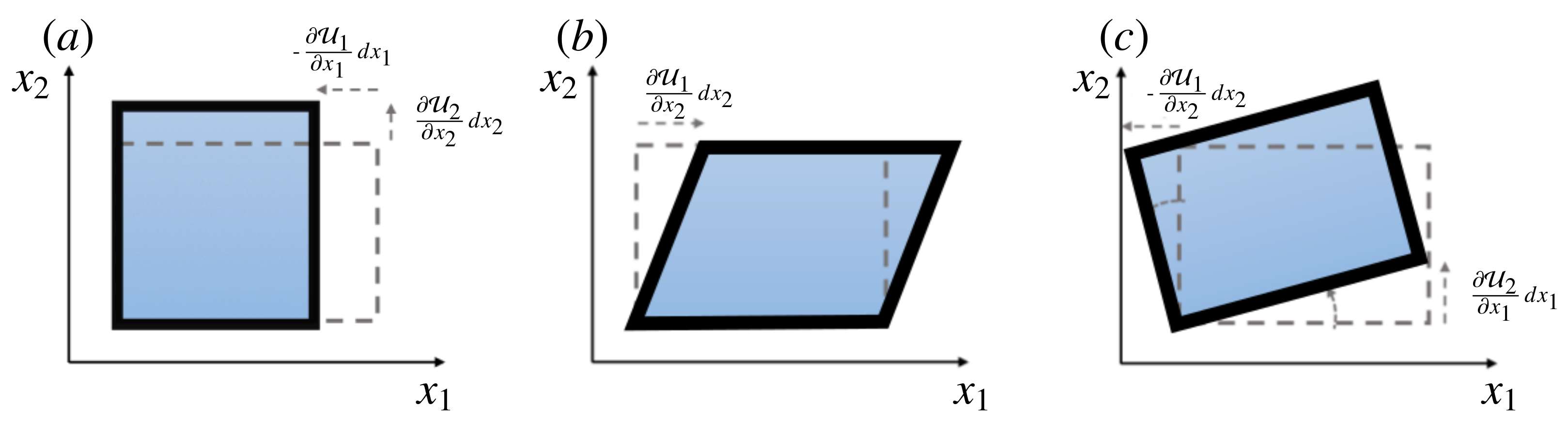
These transformations are illustrated with some elementary examples in
Figure 3. We note that the triple decomposition (
2) entails a considerable level of effort and the technique that is outlined here is presented in greater detail in [
24].
The main difficulty of the triple decomposition (
2) lies in the calculation of the pure-shear tensor,
, since the other two tensors are computed straightforwardly by subtracting
from
. The decomposition (
2) must be applied in an appropriate reference frame that originates from a specific point in the flow field. This reference frame is called the “basic reference frame” (BRF). In the BRF, an effective pure-shear motion is shown “in a clearly visible manner” set by the condition (
20), and the effect of extraction of a shear tensor is maximized. In order to fulfill the latter condition, Kolář [
15] introduced an interaction scalar
that is defined by
Then, the BRF is determined from the condition
where
is the set of
orthogonal matrices, and
is the interaction scalar that is calculated from the velocity gradient tensor
, which is computed under a generic unitary orthogonal transformation
A tilde quantity represents a quantity that was evaluated in the rotated reference frame. The derivation of the orthogonal matrix (rotation matrix whose yaw, pitch, and roll angles are
,
, and
, respectively)
applied to a Cartesian coordinate
is provided in [
15], and it reads (where
and
denote the cos and sin functions, respectively)
where
,
, and
are the three rotation angles. In the procedure that was proposed by Nagata et al. [
24] to compute the BRF, these three rotation angles are varied with a uniform step size
, yielding a finite number of reference frame rotations:
, where
are three integers satisfying
,
, and
. Therefore, the determination of the accurate location of BRF requires significant computational effort as a small step size
must be used.
Our strategy instead consists in the formulation of the BRF determination as an optimization problem of the three bounded variables
,
, and
, and a fixed velocity gradient tensor,
, associated with the point
of the mesh
Here, to solve Equation (
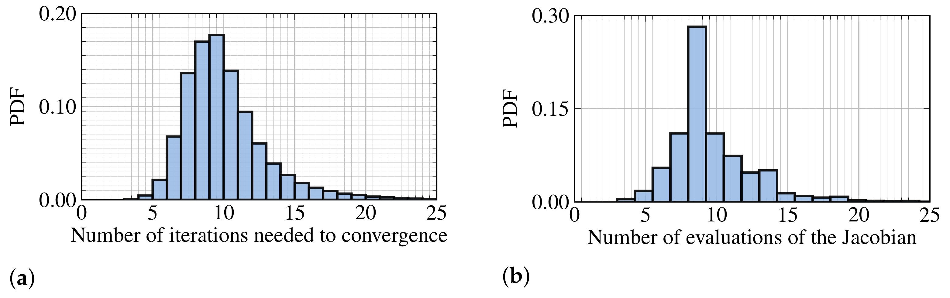
25), we use the gradient-based optimizer sequential least-square quadratic programming (SLSQP), which is an SQP-like algorithm with a Broyden–Fletcher–Goldfarb–Shanno (BFGS) update the formula for approximating the inverse of the Hessian matrix of the objective function. In practice, a free modern FORTRAN SLSQP optimizer version [
44] is coupled with our solver to achieve this purpose. To highlight the behavior of the proposed approach, we carry out a relatively small simulation while using
grid points.
In
Figure 4, we show the probability density function (PDF) of the number of iterations and the number of evaluations of the Jacobian of the objective function performed by the optimizer to locate the BRF. We observe a left-skewed tendency and peak at approximately 10 iterations, which allows for a fast and more accurate location of the BRF when compared to the previous discrete approaches [
24,
45]. When comparing the difference between the present method and the one of Nagata et al. [
24], the difference gets smaller as the step size
becomes smaller. Besides, the method (SLSQP) exhibits no sensitivity to the initial guess of
.
This step results in the velocity gradient tensor
in the BRF, and then can, therefore, be decomposed into the following constituent tensors
. Here, the residual tensor
is expressed as
where the sign function of a generic real number
x gives -1 if
, 0 if
, and 1 if
. Finally, the tensor
can be further decomposed into symmetric and anti-symmetric parts as
, where
The resulting decomposition is finally expressed in the laboratory reference frame as
for a generic tensor
. The pure-shear tensor is divided into its symmetric
and anti-symmetric
counterparts, i.e.,
The symmetric-shear tensor
, along with normal-strain-rate tensor
, recovers the strain-rate tensor
, while the anti-symmetric-shear tensor
m along with rigid-body-rotation tensor
constitutes the rotation-rate or vorticity tensor, i.e.,
From Equation (
29), we notice that the pure-shear motions contribute to both vorticity and strain-rate.
Figure 2 illustrates the shape of the local streamline that is associated with the tensors associated with the triple decomposition in the
plane [
43]:
: Non-rotational geometries (), the tensor has only real eigenvalues; and,
: Rotational geometries (), the tensor has complex eigenvalues, the flow is locally rotational, and the three tensors , , and are in general non-zero.
6. Results and Discussion
In
Figure 5, we show the isocontour lines (of the logarithm) of the second,
and third,
, invariants for the values of the turbulent Mach number,
, considered in the present database. As expected, all of the joint PDFs exhibit the classical tear-drop shape as in the incompressible case, with a statistical preference in the
SFS and
UNSS quadrants. Within these quadrants, the statistical points are mostly aligned with the right branch that corresponds to
. The compression motion tends to reveal a stronger alignment with the right branch, as indicated by a rather sharp joint PDF with the curve
[
27].
Table 2 provides a quantitative comparison between the conditional data of each case in percentage, distributed over the possible local topologies (the row sum is 100%). As expected, the most frequently occupied regions are the
SFS and
UNSS regions, which are dominated by positive enstrophy and strain productions. Furthermore, the probability of occurrence of each topology in the almost incompressible case with
is very close to that found in the compressible turbulence. This fact proves that (i) the dilatation has a negligible effect on the occurrence of each topology and (ii) compressibility marginally affects the invariant statistics. The occupancy of the non-rotational region that is characterized by
is close to the sum of the conditional data of the
UNSS and
SNSS topologies.
For the sake of clarity, from this point onward, we adopt the notations and to indicate the strain-rate magnitude and vorticity magnitude (or enstrophy), respectively, of a generic tensor with symmetric, , and anti-symmetric, , parts. Note that from the construction of . Therefore, the strain-rate magnitude, , and rotation-rate magnitude, , (in the sense of Frobenius norm) are expressed in terms of , , , and .
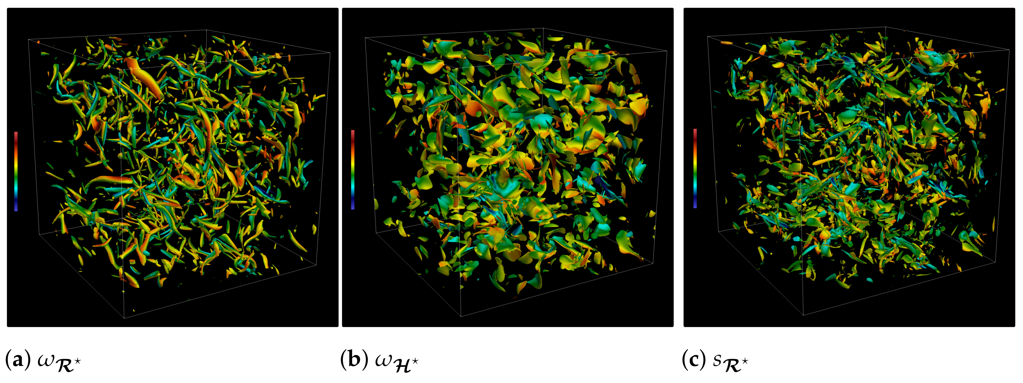
To show the flow structures that are deduced from the triple decomposition of
, in
Figure 6 we plot the isosurfaces for the four constituents of vorticity and strain-rate for
. A vortex filament is viewed as a vortex tube of variable cross-section for
, as shown in
Figure 6a. We note that the shearing motion contribution for the vorticity and strain production corresponds to sheet-like structures, which is a marker of high energy dissipation/strain rate regions [
46], as shown in
Figure 6b. In contrast, the instantaneous snapshot of the
isosurface shows a highly intermittent turbulence in space.
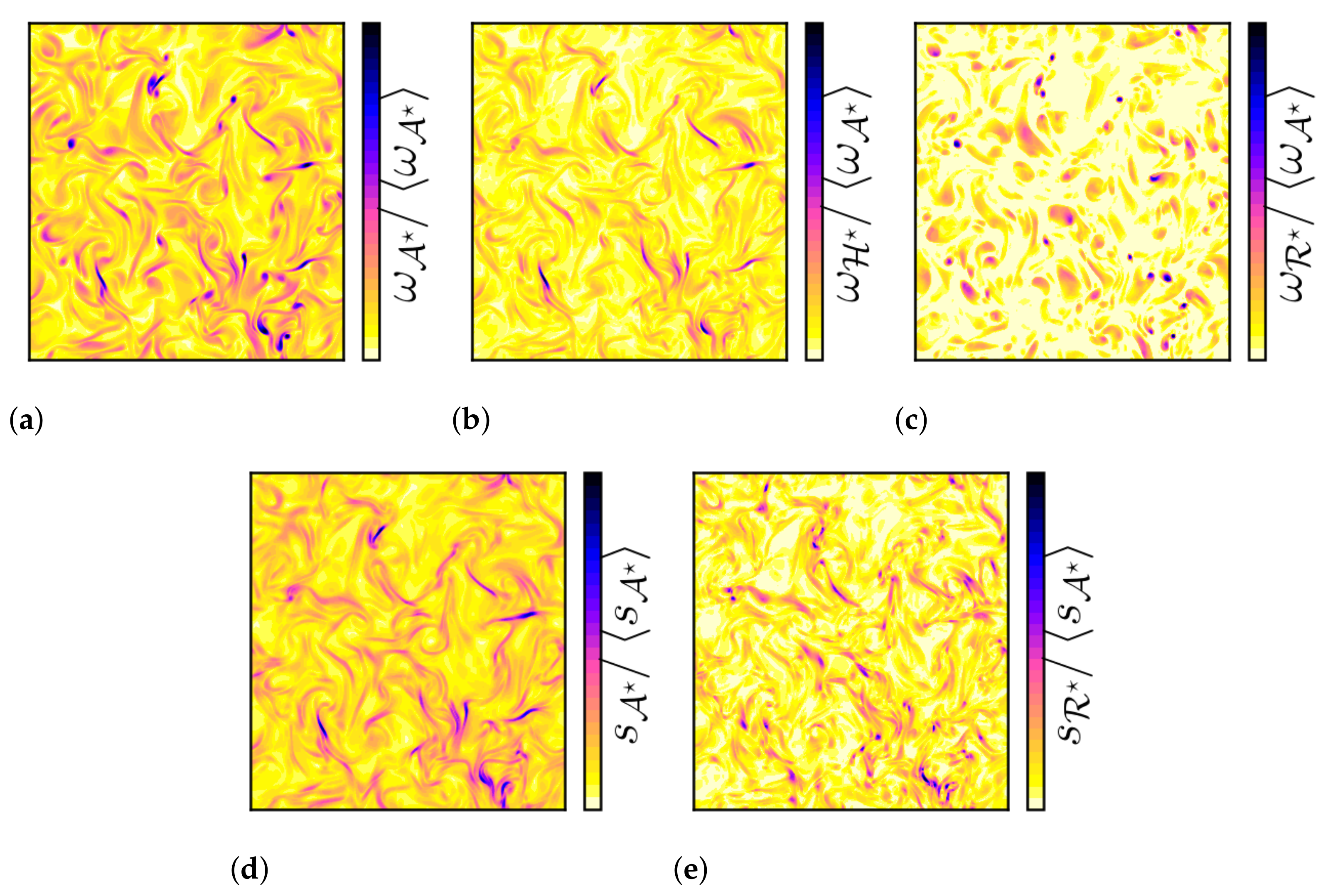
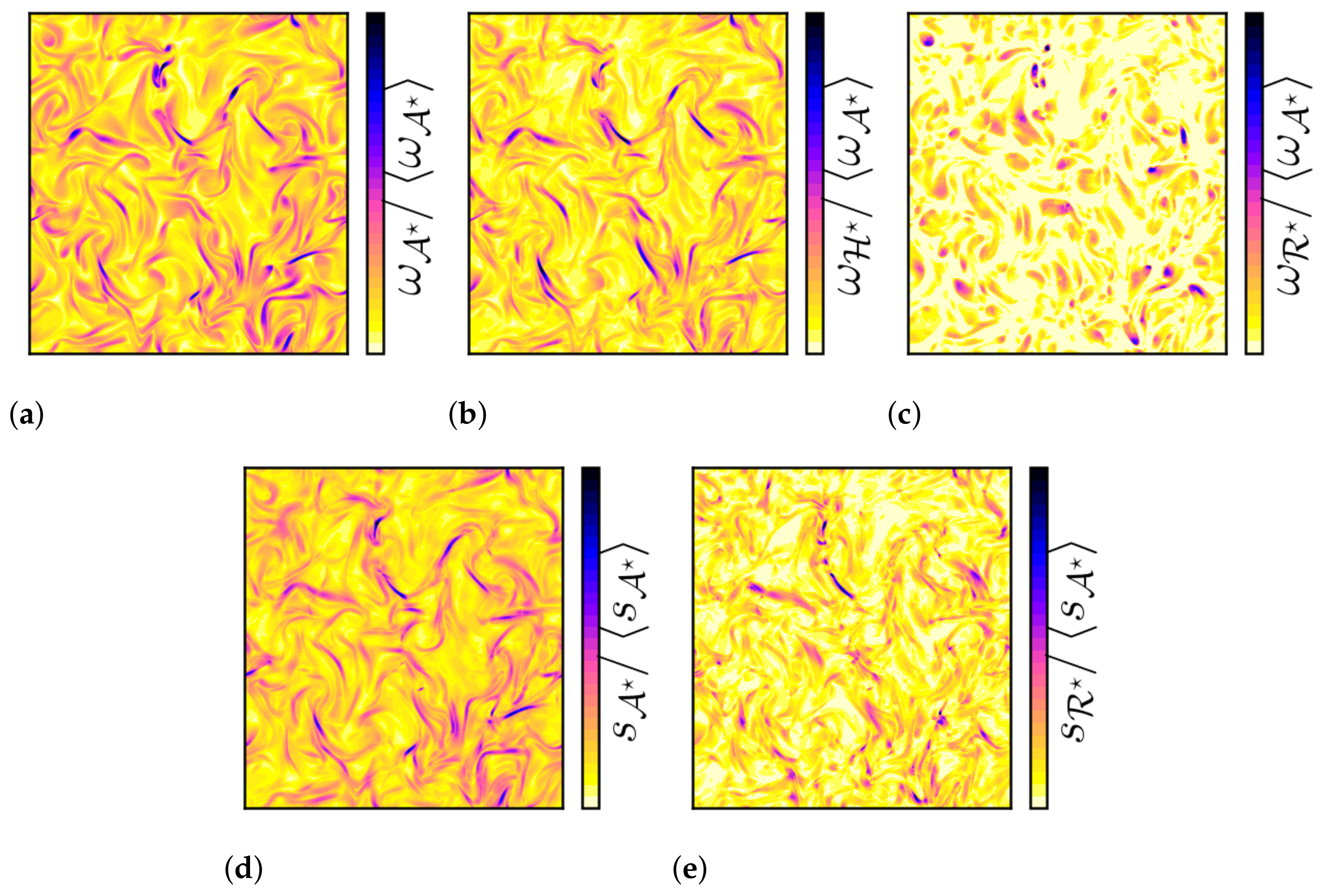
A possible two-dimensional illustration of the decomposition of vorticity and strain rate magnitudes is presented in
Figure 7 for
(an almost incompressible case) and
Figure 8 for
(an example of a compressible case). All of the other cases display similar patterns. In the following, the focus is,
mainly, put on the qualitative description of the decomposition for the compressible case.
Because the vorticity is a local characteristic of the flow and includes both the solid body rotation and the shearing motion of a fluid element, we can isolate the two effects by comparing
Figure 8a,b.
Figure 8b indicates that the vortices are frequently located in high shear zones.
This implies that the criteria of vortex detection (e.g., the
Q-criterion), which simultaneously detects shear layers and vortex regions, sometimes yields results that are difficult to interpret. Indeed, they exclusively locate a region that is to be either dominated by strain or by rotation. Regions of high intermittency are associated with large values of
(vortex with a strong-body rotation) and
(strain with a strong-body rotation), as depicted in
Figure 8c–e.
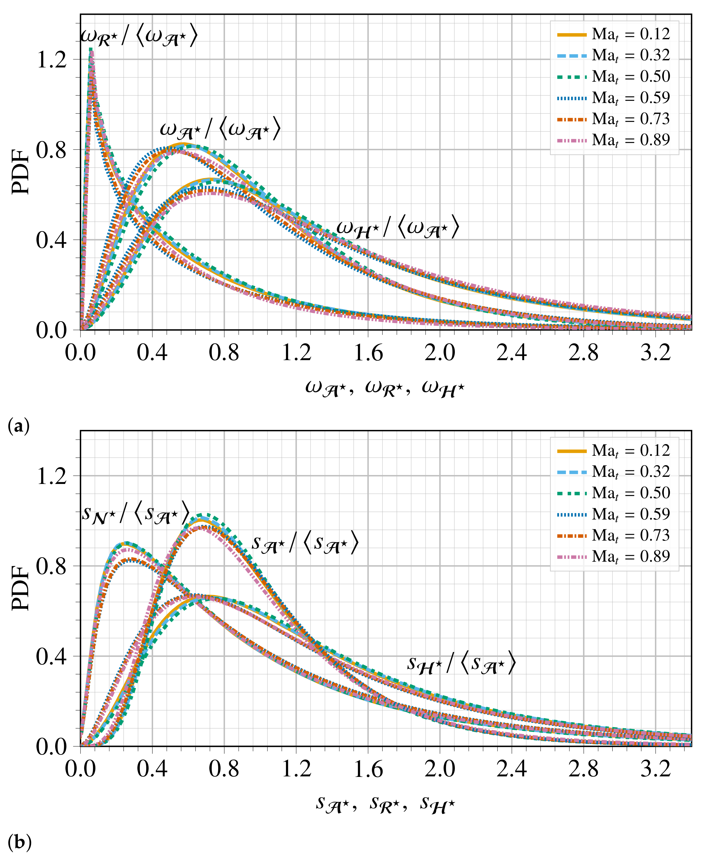
To deepen our investigation of the statistical properties of the triple decomposition, in
Figure 9 we report the normalized
and
and their components
,
,
, and
. As in the incompressible case, all of the PDFs exhibit a two-stage evolution of their shapes, where they first increase up to a peak, and then decrease slowly to lower values. The effect of compressibility is slightly significant for
. The PDFs of
and
become wider and extend slowly to much higher values. Moreover, the PDF of the strain-rate magnitude has a less wide tail at higher values and it is more intermittent in comparison to the rotation-rate magnitude at smaller and moderate values. This observation, which holds true independently from the compressibility intensity considered within our investigation, is a well-known characteristic of spatial intermittency [
47,
48]. The same figure shows that the pure-shear magnitudes
and
exhibit a wider tail and a flatness, and they are more intermittent than the other components. As a result, one can conclude that the pure-shear motions have a greater contribution in the heavy-tailed PDF of the VGT magnitude. In particular, the large probability values of
are mostly associated with the shear, rather than the rigid-body rotation. The rigid-body rotation strain magnitude,
, first reaches a peak at
, and it decreases while the pure-shear contribution increases to reach its maximum value at
, as the strain-rate magnitude. The compressibility seems to slightly affect the fat tail of the PDFs for small values of
and
s.
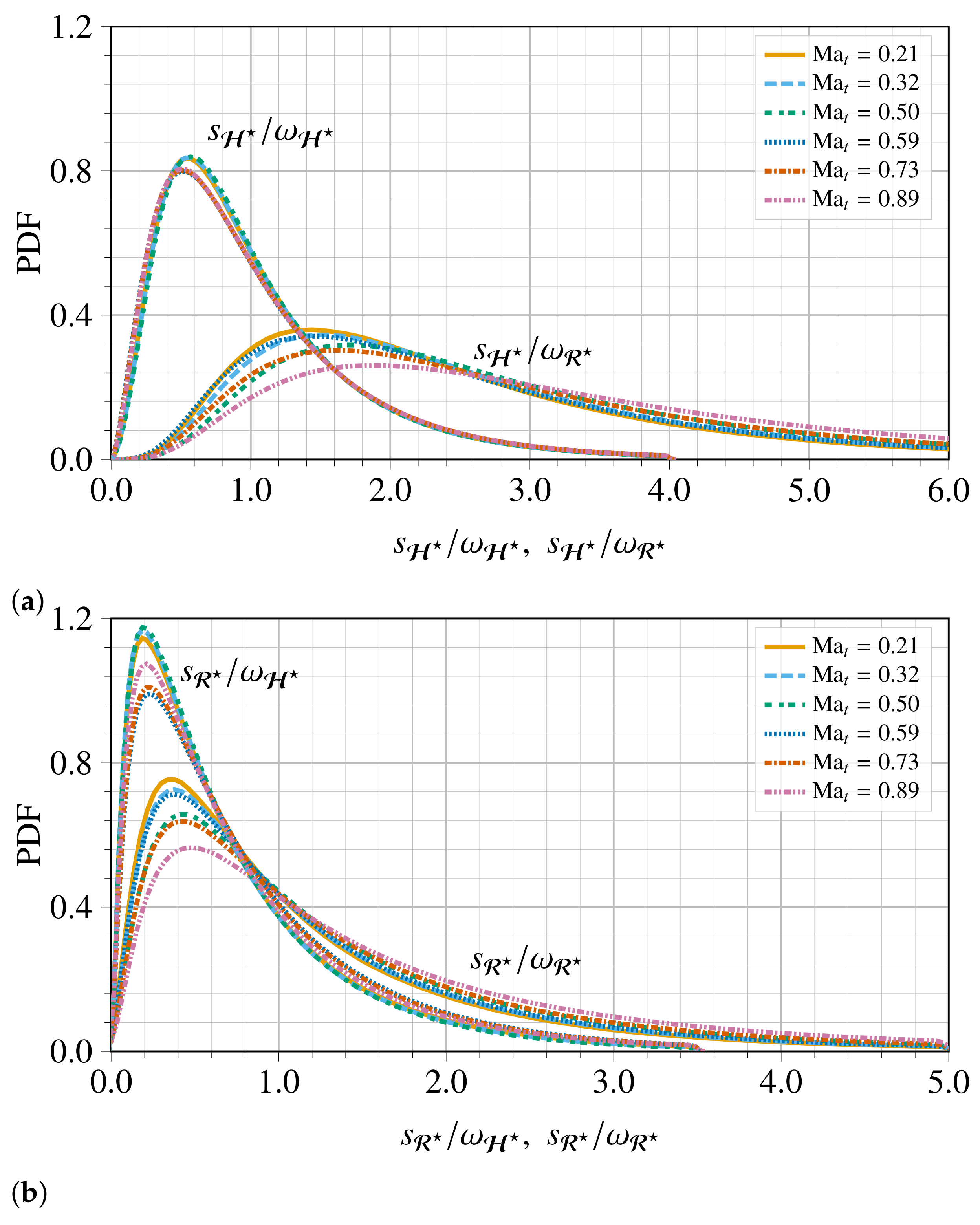
Figure 10 shows the PDFs of the ratio
,
,
, and
for various
. These distributions suggest that vortices are most probably located in regions where the shear-strain rate is equal to, or larger than, the maximum vorticity of the vortices. However, the most probable case is the one of low shear, which confirms that the vorticity is not always a good indicator for measuring the strength of the local swirling. Moreover, as the mode of the PDFs of the four quantities portrayed in
Figure 10 is likely associated with the intensity of the compressibility effects. The overall mode of the distribution increases by increasing
.
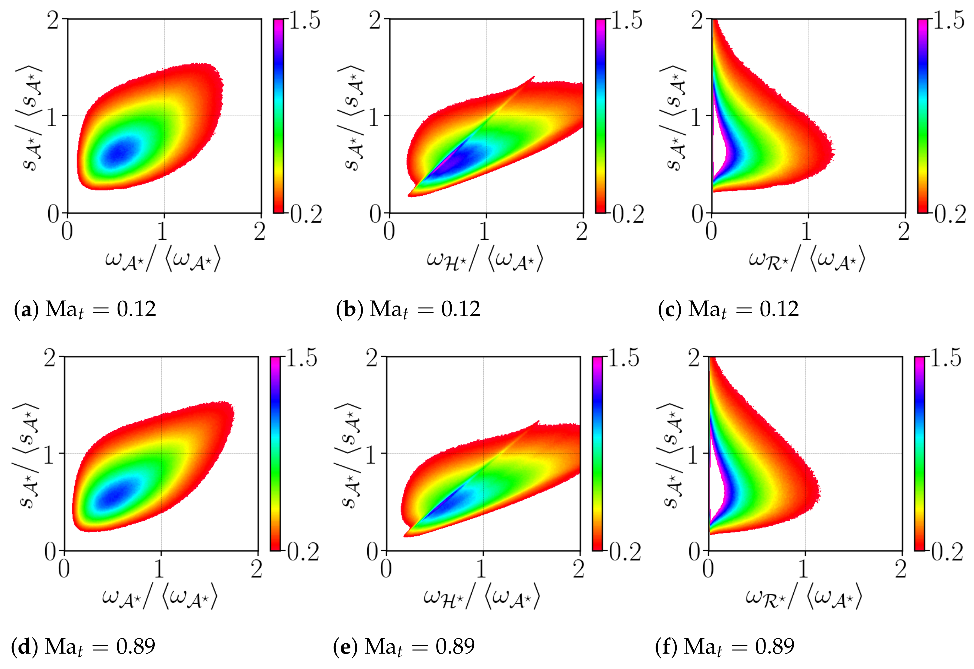
We further address the coupling between the vorticity and strain by looking at the two-dimensional joint PDF of the vorticity magnitude (enstrophy) and its two components against the total strain rate.
Figure 11a,d indicate that strong vorticity coexists with strong strain, even though the correlation between
and
seems to be rather weak, and even weaker for lower
[
37]. The shearing-motion contribution in the production of enstrophy is likely more correlated with the strain rate than the rigid-body rotation. In order to quantitatively assess this feature, we compute the Pearson’s bi-variate coefficients of correlation between each component. This coefficient detects any existence of linear relations between pairs of variables and it reads
where
stands for the covariance of the variables
x,
y, whereas
and
are their respective standard deviations.
We notice that the high correlation between
and
is mostly due to the shearing-motion of the vorticity, as depicted in
Table 3, and the correlation between strain rate and component of vorticity is almost constant, regardless of the intensity of the compressibility.


