Article

Two-Phase Turbulence Statistics from High Fidelity Dispersed Droplet Flow Simulations in a Pressurized Water Reactor (PWR) Sub-Channel with Mixing Vanes

Department of Nuclear Engineering, North Carolina State University, Raleigh, NC 27695, USA
*
Author to whom correspondence should be addressed.
Fluids 2021, 6(2), 72; https://doi.org/10.3390/fluids6020072
Submission received: 16 December 2020 / Revised: 24 January 2021 / Accepted: 1 February 2021 / Published: 6 February 2021

Abstract

:
In the dispersed flow film boiling regime (DFFB), which exists under post-LOCA (loss-of-coolant accident) conditions in pressurized water reactors (PWRs), there is a complex interplay between droplet dynamics and turbulence in the surrounding steam. Experiments have accredited particular significance to droplet collision with the spacer-grids and mixing vane structures and their consequent positive feedback to the heat transfer recorded in the immediate downstream vicinity. Enabled by high-performance computing (HPC) systems and a massively parallel finite element-based flow solver—PHASTA (Parallel Hierarchic Adaptive Stabilized Transient Analysis)—this work presents high fidelity interface capturing, two-phase, adiabatic simulations in a PWR sub-channel with spacer grids and mixing vanes. Selected flow conditions for the simulations are informed by the experimental data found in the literature, including the steam Reynolds number and collision Weber number ( W e c = { 40 , 80 } ), and are characteristic of the DFFB regime. Data were collected from the simulations at an unprecedented resolution, which provides detailed insights into the continuous phase turbulence statistics, highlighting the effects of the presence of droplets and the comparative effect of different Weber numbers on turbulence in the surrounding steam. Further, axial evolution of droplet dynamics was analyzed through cross-sectionally averaged quantities, including droplet volume, surface area and Sauter mean diameter (SMD). The downstream SMD values agree well with the existing empirical correlations for the selected range of W e c . The high-resolution data repository from the simulations herein is expected to be of significance to guide model development for system-level thermal hydraulic codes.

1. Introduction

Pressurized water reactors (PWRs) are designed with safeguard systems to withstand and/or mitigate the effects of several accident scenarios that are postulated to occur during their lifecycle [1]. Among them, the large break LOCA (loss-of-coolant accident), wherein the core gets depressurized and loses its coolant due to a piping failure, is the most challenging accident to analyze and model [2]. The thermal hydraulic characteristics during the post-LOCA reflood transients are described by either the inverted annular flow boiling (IAFB), which has a steam volume fraction (or void fraction) of less than 50% [3,4], or the dispersed flow film boiling (DFFB) regime, with void fraction greater than 90% [5,6]. As unanimously reported by an extensive set of experiments [1,7], the DFFB regime persists through the major length of the axial core for most reactor reflood conditions, making it the primary regime of interest for analysis, modeling and overall PWR safety margin characterization.
Spacer grids and mixing vanes play an especially critical role in the overall thermal hydraulics of the PWR core for the DFFB regime [8,9]. Single-phase steam experiments by Hochreiter et al. [10] reported augmentation to the convective heat transfer in the immediate downstream vicinity of spacers, owing to the turbulent kinetic energy (TKE) imparted by the mixing vanes, based on which empirical correlations were developed to account for the phenomena in system thermal hydraulic (STH) codes [11,12]. For two-phase dispersed droplet flow, the increase in heat transfer is further pronounced [12,13,14] primarily due to inertial impaction of the droplets with the spacers, resulting in quenching, which is semi-mechanistically modeled in STH codes [15], and droplet breakup or deformation. The latter phenomenon provides massive positive feedback to several heat transfer paths [16], viz., convective heat transfer enhancement from mass transfer due to rapid evaporation of smaller droplets, radiation heat transfer from fuel rods to droplet surface and interfacial heat transfer from steam to droplets. The heat transfer increase across spacers has been empirically correlated with the observed decrease in the Sauter mean diameter (SMD) of the droplets [17], which provides a statistical measure to characterize their morphology and is accounted for in STH codes [18,19]. It was noted by Hochreiter et al. [16], however, that the aforementioned models for the DFFB regime have considerable implicit measurement uncertainty and model uncertainty related to their implementation in STH codes.
Other phenomena pertinent to DFFB thermal hydraulics is dispersed phase-induced turbulence, which is hitherto not rigorously studied and modeled for in STH codes, owing to measurement difficulties. The presence of droplets decreases the effective hydraulic diameter for the continuous steam flow, which is expected to increase the overall TKE. Further, it can be conjectured that droplet breakup and/or deformation by the spacer-grids and mixing vane structures will result in increased feedback to TKE in the downstream region. As noted by Behzadi et al. [20], turbulence contribution due to the dispersed phase is a superposition of shear-induced turbulence, owing to the boundary layer developing around the interface, and the droplet- (or bubble-) induced turbulence, due to perturbations of the interface and small scale structures in the wake arising from the relative motion. The models developed to account for turbulence in dispersed two-phase flows, however, are based on limited experimental data (e.g., [21,22,23]) and subject to measurement uncertainty and have limited predictive capability [24,25,26,27]. Owing to the axiomatic limitations of the experiments, high-resolution, direct numerical simulation (DNS) provides an alternative viable source for the much-needed data for the two-phase flow turbulence modeling of the DFFB regime (or dispersed two-phase flows in general).
The rapid advent of high-performance computing (HPC) systems has only recently enabled excursions into large-scale interface-resolved simulations of complex two-phase flows. Using the strongly parallel scaled, finite-element-method-based code—PHASTA (Parallel Hierarchic Adaptive Stabilized Transient Analysis) [28,29]—and the level-set interface capturing method [30], two-phase simulations have been performed for conditions representative of PWR flow regimes, including bubbly flows [31,32,33], slug-to-churn flow [34] and the DFFB regime [35] (from our prior work). Interface tracking method [36] and immersed boundary method [37] have also been used for simulating bubbly flows; however, their challenging numerical implementation precludes applicability to complex geometries and complex interface topologies. Irrespective of the method used, the high-fidelity data made available by DNS simulations, coupled with the machine learning (ML)-based modeling frameworks [38], has proven to be valuable for constructing data-driven and physics-informed models for turbulence closure [39,40] and two-phase flows (e.g., [41,42]). The success of data-driven models, however, is a strong function of the fidelity, resolution and quantity of data available from experiments or DNS simulations. Extracting the flow features from the experiments, such as instantaneous velocity and pressure gradients, with high spatial and temporal fidelity remains a challenge. Data extraction from DNS or large-eddy simulations (LES) also poses a significant bottleneck, since data I/O significantly overshadows the scaling performance of the code. Writing data to disks is the most time-consuming operation, which is the reason that restart data from the simulations is written sparingly to files. The limited availability of data precludes the development of data-driven models for engineering flows (e.g., in PWR geometries).
In this work, we significantly extend the analysis presented in Saini and Bolotnov [35]. Interface capturing simulations were performed using PHASTA [29] for conditions representative of the DFFB regime. The two-phase dimensionless properties in the present work were for a steam-water system at 30 psi (see Table 1), while in [35] it was chosen to represent an air-water system at atmospheric conditions, and three sets of simulations were performed for collision Weber number, W e c { 40 ,   55 ,   80 } (Equation (14)). Further, data were collected from the simulations at a significantly enhanced spatial resolution, which enabled detailed cross-sectional analysis of the turbulence statistics and allowed unprecedented insight into the effects of spacer-grids and mixing vanes and the presence of droplets on turbulent flow features. Axial evolution of the droplet dynamics was also analyzed through droplet volume, surface area and Sauter mean diameter and compared with existing empirical correlations for all Weber number cases. Both instantaneous and time-averaged data from the simulations were archived and are intended to be used for training machine-learning-based turbulence or STH closure models.

2. Numerical Setup

Details of the numerical method, including the challenges encountered for large-scale representative DFFB simulations, were discussed in detail in Saini and Bolotnov [35] (and Saini [43]). Here, we provide a brief overview of the numerical method, focusing on the details specific to the presented simulations.

2.1. Governing Equations

The computational fluid dynamics (CFD) tool used for the simulations is PHASTA, based on the continuous Galerkin finite element method (CG-FEM) and stabilized using the streamline upwind Petrov-Galerkin (SUPG) method [44]. Owing to the CG-FEM formulation and advanced domain decomposition strategies [45], PHASTA yields excellent strong scaling on large-scale supercomputers [46]. Owing to the low Mach number characteristic of post-LOCA DFFB conditions [13], compressibility effects can be neglected. Thus, the governing equations are the incompressible Navier-Stokes (INS),
u = 0
ρ ( u t + u × u ) = p + × τ + f + κ δ ( ϕ ) n ;   τ = μ (   u +   u T )
For two-phase flow simulations, PHASTA uses the built-in level-set (LS) interface capturing method [47,48]. In the LS method, an additional contour field, ϕ , is transported by the underlying velocity field,
ϕ t + u ϕ = 0
which allows the flow in the entire computational domain to be solved as a single fluid. The single-fluid approach is common and is also used in other popular interface capturing methods, such as front tracking or volume of fluid. Zero contour of the contour field is identified as the interface between fluids, and the properties are transitioned across the interface using a smoothed Heaviside function,
H ( ϕ ) = { 0 ϕ < ϵ 1 2 [ 1 + ϕ ϵ + 1 π sin ( π ϕ ϵ ) ] | ϕ | < ϵ 1 ϕ > ϵ }
where ϵ is the user-defined smearing length, and the properties are given as,
ρ ( ϕ ) = ρ g H ( ϕ ) + ρ l ( 1 H ( ϕ ) ) μ ( ϕ ) = μ g H ( ϕ ) + μ l ( 1 H ( ϕ ) )
Surface tension, included as the last term in the momentum Equation (2), is modeled as a smeared continuum force [49] using the one-dimensional delta function,
δ ( ϕ ) = { 0 ϕ < ϵ 1 2 ϵ [ 1 + cos ( π ϕ ϵ ) ] | ϕ | < ϵ 0 ϕ > ϵ }
The normal to the interface and the curvature, required for the surface tension force term, are calculated using the normalized gradient and the divergence of the LS field,
n = ϕ | ϕ |
κ = ϕ | ϕ |
For accurate calculation of surface tension, it is imperative that the LS field maintains an accurate signed distance function, especially within the | ϵ | < ϕ region, where Equation (6) is non-zero. The signed distance property, however, is rendered inaccurate due to the LS advection, Equation (3). To restore this property an additional hyperbolic partial differential equation is solved in pseudo-time, τ [50],
ϕ d τ + w ϕ d = s i g n ( ϕ 0 ) ;       w = s i g n ( ϕ 0 ) ϕ d | ϕ d |
where ϕ d is the corrected signed distance LS field that is arrived at on successive iterations, while ϕ 0 is the initial solution supplied to the above equation, obtained after the LS advection step. The sign function in the above equation is also spread across the zero contour to avoid numerical instabilities,
s i g n ( ϕ 0 ) = { 1 ϕ 0 < ϵ ϕ 0 ϵ + 1 ϵ sin ( π ϕ 0 ϵ ) | ϕ 0 | < ϵ 1 ϕ 0 > ϵ }
In practice, 15–20 iterations of Equation (9) were performed to restore the distance property near the interface, with a CFL (Courant-Friedrichs-Lewy) between 1–2, using an implicit solver in PHASTA. For highly turbulent dispersed flow simulations where the length of the computational domain is significantly large compared to the droplets/bubbles, an inordinate amount of iterations of Equation (9) or a high CFL is required to correct the distance field in the peripheral regions of the domain. Further, for the particular simulations herein, the solution of Equation (9) near the boundary where droplets collide with the spacer-grid and mixing vane structures leads to further complication owing to the compression of the LS field, demanding a low CFL in the vicinity of the interface to ameliorate numerical difficulties. An adaptive time-stepping algorithm was therefore introduced to tackle these problems. The reader is referred to our earlier work [35] for a detailed exposition of these problems encountered with the representative DFFB simulations and their novel solution.

2.2. Geometry and Simulation Properties

As alluded to earlier, spacer-grids and mixing vanes play a critical role in the overall thermal-hydraulic response of the post-LOCA DFFB regime. Accordingly, the simulations are designed to study the detailed hydrodynamics of droplets, including their collision and breakup, in the vicinity of spacer-grids and mixing vanes. Figure 1 shows the simulation geometry with dimensions and spacer and mixing vane features representative of a typical PWR sub-channel. The simulations assume lateral periodicity, thus neglecting cross-flow effects. An inflow boundary condition, as described later, is assigned at the upstream axial boundary and zero pressure is assigned at the downstream axial boundary, while zero-slip boundary conditions are prescribed on the curved rod walls. The hydraulic diameter of the domain, not accounting for the internal structures, is D h = 12.976 mm. The leading edge of the spacer-grid is at an axial distance of 0.23 D h , and the trailing edge of the mixing vane is at 1.4 D h , while the total length of the computational domain is 3.08 D h .
The bulk Reynolds number for all the simulations included in this work is maintained at R e b = 11 , 822 , while the corresponding friction Reynolds number is R e τ 243 , which are defined, respectively, as
R e b = ρ g U D h μ g
R e τ = ρ g u τ D h 3 μ g
where U and u τ = τ w / ρ g are the bulk mean velocity, as measured at the inlet cross-section, and the friction velocity, respectively. The wall shear stress, τ w , is estimated a priori from the Darcy friction factor [51] based on the bulk Reynolds number. As noted in [35], the rationale for the choice of characteristic length, equal to D h / 3 , in the definition of R e τ is that it yields a value close to the shortest dimensionless wall distance from the center of the subchannel. This is consistent with the convention followed by Lee et al. [52] for typical channel flow, which makes subsequent analysis intuitive and convenient.
To generate the computational mesh, the first node of the walls, including rods and internal surfaces, was placed at a distance of y + = 0.561 ( y = 10   μ m ), where y + is the normalized distance,
y + = y u τ ρ g μ g
The need to resolve the interface imposes stringent mesh resolution requirements, especially in the near-wall region. Accordingly, the bulk mesh resolution is in the range, ( Δ x + , Δ y + , Δ z + ) = [ 2.45 ,   4.9 ] (43.75–87.5 µm), with the finer mesh extending up to Δ x + = 336.62 (6 mm). The lowest bulk resolution is maintained to have at least 20 mesh elements across the diameter of the droplets at the inception location, guided by prior studies [53], for capturing interface curvature with reasonable accuracy. Further, extended boundary layers were applied on all internal surfaces with a growth factor of 1.2, extending up to a distance of Δ y + = 42.81 . The mesh consists of approximately 367.5 M tetrahedral elements, depicted in Figure 1.
DNS (or even LES) scale simulations of PWR sub-channels are usually performed on axially periodic domains [33,54], which allow the flow to develop to a quasi-steady turbulent state. Here, however, the presence of the droplets and spacer-grids and mixing vane structures preclude the option of employing a periodic domain. Therefore, single-phase simulation was first performed on a sub-channel geometry, of similar dimensions and mesh resolution, with periodic boundaries across axial ends. Instantaneous velocity data were collected from this simulation after a quasi-steady state was attained, which served as the inlet boundary condition for all ensuing two-phase flow simulations. The prescribed velocity profile was captured at the spatial resolution of the mesh shown in Figure 1 and at the approximate temporal resolution of the two-phase flow simulations, ensuring all relevant scales of turbulence were accounted for in the inlet profile. Note that all the two-phase simulations listed in Table 1 used the same data repository for specification of the turbulent velocity profile at the inlet.
The properties for the single and two-phase flow simulations are enumerated in Table 1. The system pressure under post-LOCA conditions is near atmospheric, 20 45   psi [16]. The density ratio of a water–steam system under these conditions is ~1000, while the viscosity ratio is ~10. For the simulations presented in this work, the two-phase properties correspond to the water-steam system at 30   psi and steam superheat of 100 K. The two-phase simulations retain the same values for the steam phase as listed in Table 1 for the single-phase simulation. Note that Table 1 also includes the properties for the simulation presented in [35], corresponding to the water-air system, with the primary difference being the higher viscosity ratio for this case. The controlled dimensionless parameters in all two-phase simulations are the bulk Reynolds number and the collision Weber number, defined as
W e c = ρ l D u d 2 σ
Spherical droplets are introduced in the flow domain at the upstream location of the spacer-grids by periodically re-initializing the local LS contour field,
ϕ ( x ) = min ( ϕ ( x ) , ( x x s ) 2 + ( y y s ) 2 + ( z z s ) 2 r s )
where r s is the radius, which, assuming monodisperse droplets, is kept constant at 0.5 mm and ( x s , y s , z s ) are the selected coordinates of the center of the initialized droplet. The size of the droplets is kept constant across all steam-water cases, while the surface tension coefficient is applied to change the W e c values. This eliminates the need for choosing different mesh resolutions for different cases, maintaining the same number of mesh elements across the diameter for all droplets initialized at the upstream location for all cases. The center coordinates are chosen based on a random sampling routine, which considers all mesh node points at the inlet cross-section as the sample space, except the nodes at a distance less than 0.75 D from the rod walls. Further, it is assumed that the droplets at the injection plane do not intersect. A minimum distance of 1.5 D is maintained between the droplet centers, and the centers lie at a distance of 0.5 D from the inlet cross-section. Note that the incident, essentially single-phase, flow specified at the inlet cross-section is modified due to the newly introduced droplets. Thus, the flow profile incident on the spacer-grid surface is a reasonable approximation of the two-phase flow profile under actual DFFB conditions. Droplet initialization was also accompanied by specification of the velocity field in the droplet interior to v s = ( u d , 0 , 0 ) , where,
u d = W e c σ ρ l 2 r s
where u d is the absolute droplet velocity and σ is the surface tension coefficient. The latter was adjusted in the simulation cases, as listed in Table 1, to ensure that the collision Weber number, Equation (14), is maintained at the user-specified value, herein chosen as W e c = { 40 , 55 , 80 } , consistent with range of W e c measured from experiments [17]. Based on these parameters, the resulting aerodynamics Weber number of the droplets was < 1 for all cases, defined as,
W e a = ρ g D u r e l 2 σ  
where u r e l is the relative velocity of the droplets with respect to surrounding steam. Since W e a is significantly less than the critical Weber number [55], the droplets are not expected to undergo deformation or breakup due to aerodynamic effects. It must be emphasized that this is in harmony with the experimentally observed spherical topology of the droplets at the upstream location of the spacer-grid structures in the upper portions of the PWR channel [17,56].
More details on the droplet injection routine, the rationale for selecting the droplet parameters, accompanying assumptions and their relevance to the experiments can be found in [35,43] and are not reiterated herein for brevity.

3. Results and Discussion

All simulations were performed on the Mira supercomputer at Argonne National Laboratory [57]. The mesh for the single-phase simulation was split into 16,384 partitions and run on 128 nodes, while that for the two-phase simulations was split into 131,072 partitions and run on 2048 nodes. For the two-phase cases, the staggered flow level-set iteration approach, described by Nagrath et al. [30], was used to advance the solution. The tolerance on the continuity and momentum equations was specified to be 10 8 , with a maximum of thirty Newton’s iterations performed on the linearized system of equation. The level-set re-distancing equation, Equation (9), is solved after each step of the flow solve and LS advection step to correct the LS field in the interface vicinity, limiting the number of iterations in pseudo time to a maximum of 25 steps. The maximum time-step size for the flow and LS advection equations was 1 µs, while the re-distancing solution was assigned a constant pseudo time-step size of 5 µs. For property smearing, surface tension force term and the re-distancing equation, the smearing length, was ϵ = 87.5 µm, equal to the maximum resolution of the mesh.
The water-steam cases with different collision Weber numbers, labeled {We40, We55, We80} in this study, were run for a total simulation time of t = { 14.75 ,   13.65 ,   13.35 } ms and the global droplet volume fractions for the cases at these time stamps were {3.14, 3.12, 2.91}%. Figure 2 shows the instantaneous velocity contour plots, at chosen longitudinal and lateral cross-sections, and the droplet distribution for the We40 and We80 cases, at t = 14.75 and 13.35 ms, respectively. Juxtaposition of these two extreme cases reveals important differences in the droplet dynamics, emphasizing the role of upstream collision Weber number on the axial evolution of droplet morphology. The observed downstream droplet diameter for the We40 case is evidently larger than the We80 case. Inertial impaction and subsequent breakup lead to the visibly small diameter of droplets in the downstream region for the We80 case. For the We40 case, however, the droplets have the tendency to accumulate into larger blobs and also develop a liquid film over the leading edge of the spacer-grid surface, owing to a higher surface tension force coefficient. As noted by Cheung et al. [17], a smaller downstream average droplet size (or Sauter mean diameter) correlates with a higher heat transfer coefficient, owing to a corresponding increase in surface area. Thus, although the current simulations are adiabatic, it can be conjectured that the heat transfer coefficient for the We80 case will be higher as compared to the We40 case.
Velocity contours on the lateral cross-section located at x / D h = 1.85 are also shown in Figure 2. The interface or the zero contours of the level-set are highlighted in black on the plane (see attached animations for time-evolving profile). The mixing vanes have the tendency to push the droplets towards the peripheral regions of the domain. In actual DFFB experiments, the droplets may never contact the rod walls owing to the Leidenfrost effect [16,58]. Inability to model the Leidenfrost effect remains one of the implicit assumptions of the present simulations, which can have significant consequences on the overall heat transfer coefficient. The stark difference in the velocity magnitude inside the enclosed volume of droplets and in the surrounding gas is evident on the lateral cross-section, highlighting the high relative velocity of the surrounding steam. Owing to the higher density of the liquid in the droplet volume, the velocity contour profile in the enclosed zero-contour is visibly uniform, as compared to the surrounding gas.

3.1. Turbulence Analysis

A detailed insight into the effects of spacer-grids and mixing vanes and that of droplets on the continuous phase turbulence is essential for subsequent modeling. The data collection and subsequent averaging method in this work follow the methodology described in Saini et al. [35]. The spatial resolution of the collected data, however, is significantly increased herein, which allows the construction of detailed contour maps and axial evolution of the first-order turbulent statistics. For the necessary high throughput of the data being written to the files, adhoc, advanced message passing interface (MPI) tools were implemented in PHASTA (see [43] for details).
Figure 3 shows the configuration of the “virtual probes” placed in the computational domain, based on a priori estimates, independent of the underlying mesh. The probes are organized into 30 cross-sectional planes, placed along the axial length at equidistant locations. In terms of the distance non-dimensionalized by friction velocity, Equation (13), the probes are at a location of Δ x + = 74.8 , which is a reasonable resolution from a RANS modeling perspective. At each plane, the probes are organized into 20 loci spanning each quadrant, which run perpendicular to the rod wall profile, as highlighted in red in Figure 3. Thus, the configuration of probes is homogeneous in each quadrant, which is desirable for obtaining subsequent wall-normal trend of statistical quantities. The organization of the probes in the wall-normal direction is similar to the mesh configuration. The first probe is placed at a distance of Δ y + = 0.56 off the wall, and a growth factor of 1.2 is applied for the subsequent probes. Overall, each plane has 2960 probes, while the entire domain has 84,908 probes, not accounting for the extraneous probes in the spacer-grid and mixing vane material.
As given by Pope [59], an estimate for the Kolmogorov time scale, τ η , can be obtained from the corresponding bulk Reynolds number,
τ 0 l 0 u 0 = D h U = 1.85   ms τ η R e b 0.5 τ 0 = 17.06   μ s
where τ 0 is the time-scale estimate for the largest eddies with corresponding length scale, l 0 , equal to the hydraulic diameters and velocity scale, u 0 , equal to the bulk mean velocity. Viscous dissipation commences at the Taylor microscale, which gives the scale of the smallest eddies, on the energy spectrum, estimated as,
τ T = 15 τ η = 0.06   ms
Data were written from the simulations at each time step, where Δ t = 1 µs, for each probe, ensuring that the Kolmogorov scale eddies were captured by the data, based on the above estimates. Further, data were collected, and subsequently time-averaged, for the We40 and We80 case for an approximate time window of 3.38 ms ensuring that the eddies corresponding to the Taylor length scale are sufficiently resolved (~factor of 56). Note that, considering the local flow conditions near internal structures and the droplets, the above estimates may no longer be valid. However, since the data are collected with a sufficiently resolved time scale and for a relatively long period, we assume that the first-order turbulent statistics are appropriately captured. It must also be noted that the data collection for the two-phase simulations was commenced after the initial batch of droplets, injected at the upstream locations, and advected beyond the trailing edge of mixing vanes.

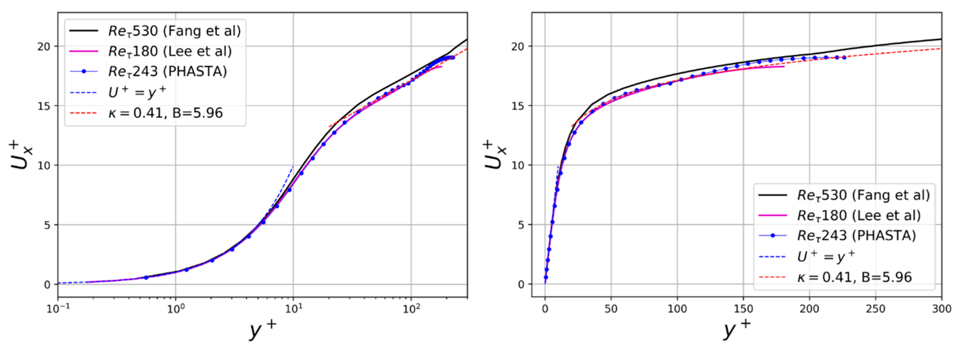
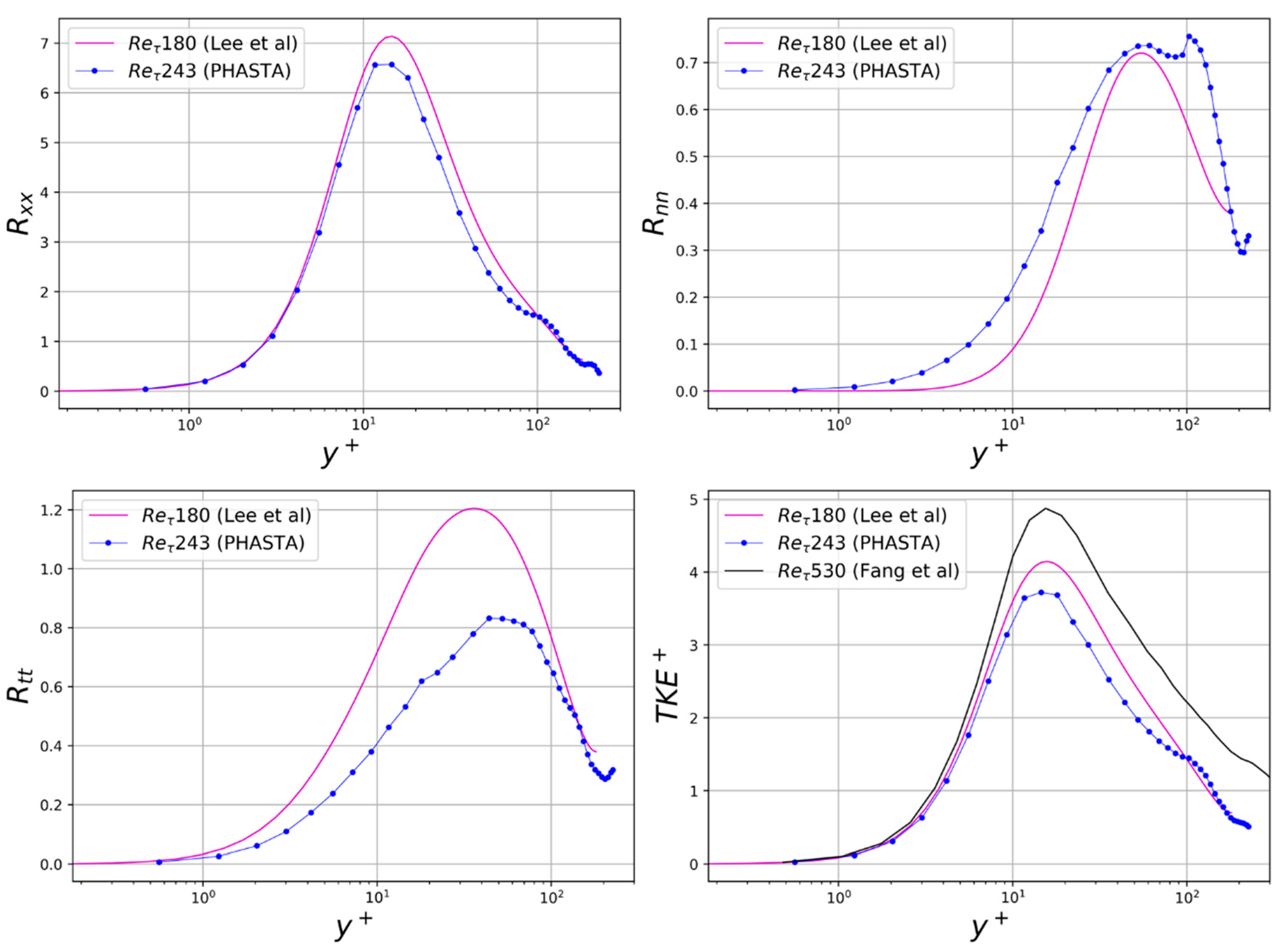
3.1.1. Verification of Inlet Turbulent Flow Features

Figure 4 shows the normalized mean streamwise velocity profile, U + = u / u τ , captured at the inlet cross-section. The droplets are introduced into the domain, with their (sphere) centers at a distance of 0.5 D from the inlet. Thus, at the inlet cross-section, the flow profile is equivalent to the fully developed single-phase case in a sub-channel without any internal structures, from which the instantaneous velocity profile is captured for describing the inlet conditions, as described earlier. Note that the mean velocity in Figure 4 is plotted as a function of the wall distance. Data from probes in each loci from all quadrants at corresponding wall distance locations are averaged, which yields the mean wall distance function trend for the selected lateral plane (for further details on data averaging, see [35]). The inlet profile was compared with the DNS results for flow between parallel plates by Lee et al. [52] and flow in a sub-channel, with similar geometrical specifications as the present work, by Fang et al. [60]. Considering the canonical linear Log law of the wall,
U + = 1 κ log ( y + ) + B
The trend in Figure 4 was fitted to obtain the parameter values of κ = 0.41 and B = 5.96 , which agrees well with values reported by Pope [59] for channel flows ( κ = 0.41 , B = 5.2 ) and that of Fang et al. ( κ = 0.43 , B = 6.7 ). Note that, as pointed out by Nagib et al. [61], the value for the above coefficients reported by different experimental and simulation source vary considerably. The sub-layer profile for the current simulations agrees excellently with the existing simulation data, emphasizing that the probe configuration is well resolved.
Figure 5 shows the normalized principal Reynolds stresses, R i j = u i u j / u τ 2 and normalized turbulent kinetic energy (TKE), T K E + = 0.5   u i u i / u τ 2 , compared with the trends obtained from Lee et al. [52] and Fang et al. [60]. Note that the normalized and tangential components of the stress terms are obtained by rotating the instantaneous lateral velocities to a wall tangential-normal ( t n ) coordinate system, as annotated in Figure 3. The trend for all components of Reynolds stress terms resembles the profile for flow between parallel plates (simple channel). However, the energy in the normal and tangential components is reorganized, with the former containing more energy in the near-wall region and the latter having lower magnitude. The streamwise and wall-normal components show peak energy in a similar range to the log-layer region for both simple channel and sub-channel cases. However, the tangential component peak is offset towards the center for the sub-channel case as compared to the simple channel. These differences and those seen towards the center of the sub-channel can be owed to differences in the geometry. The normalized TKE profile, compared with both Lee et al.’s and Fang et al.’s DNS data, shows good agreement in the observed trends. The crosswise Reynolds stress component trend for the subchannel is markedly different from that of a simple channel, included in Appendix A, Figure A1, which can be attributed to differences in geometry.

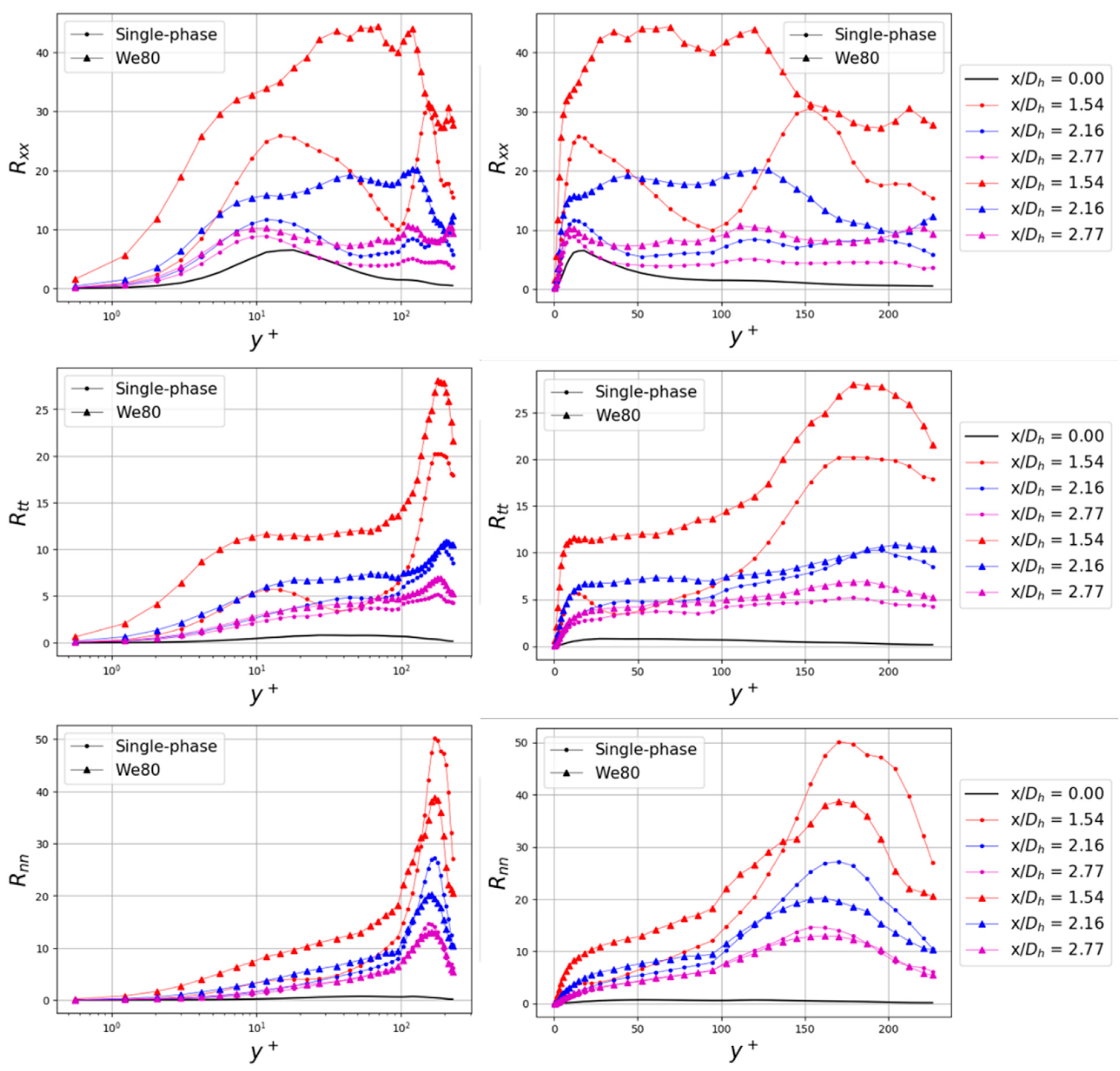
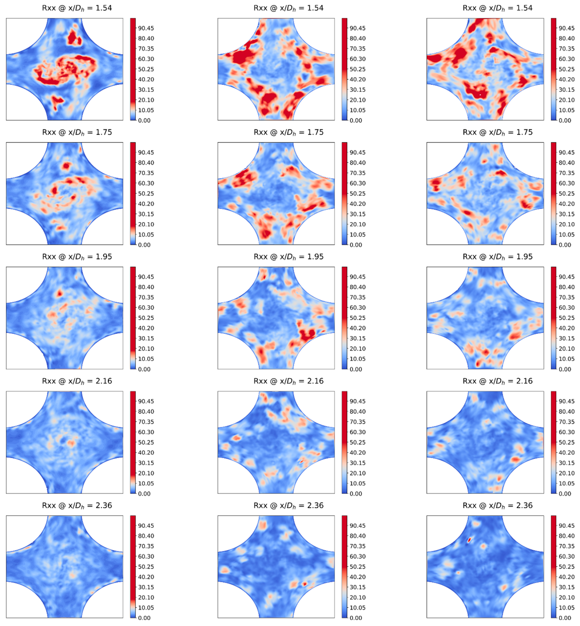
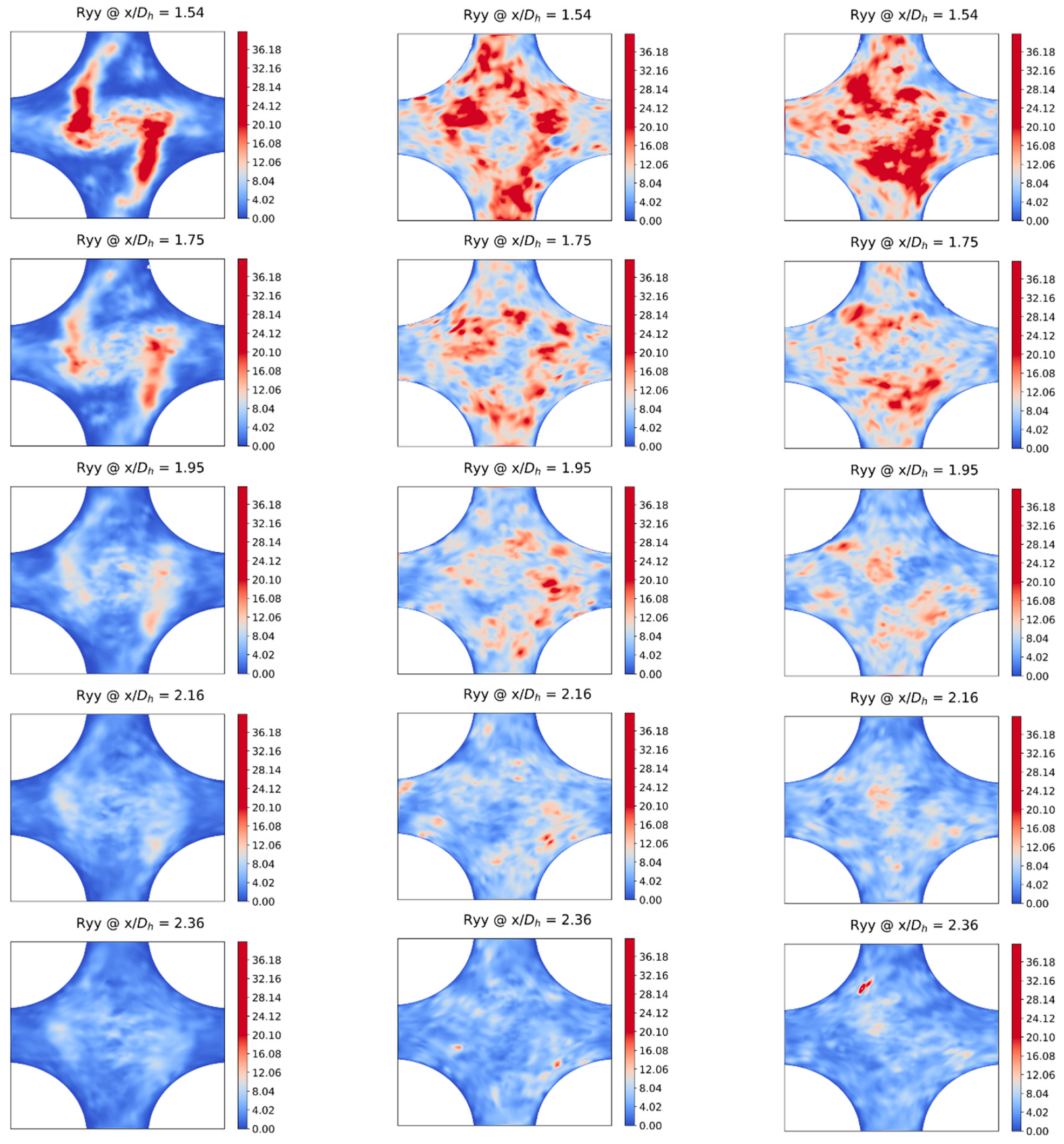
3.1.2. Effect of Mixing Vanes and Droplets on Downstream Turbulence

From a phenomenological and modeling perspective, the turbulent flow features in the downstream region, or the comparative study of the downstream profiles with respect to the upstream profiles, of the spacer-grids and mixing vane region are of specific interest. To isolate the effects of spacer-grids and mixing vanes, single-phase simulation was also performed on the same computational domain using the same database for the specification of the velocity profile at the inlet cross-section. The trailing edge of the mixing vane is located at x / D h = 1.4 . Figure 6 shows the mean normalized velocity component profile for the We80 case at three downstream locations, compared with profiles for the single-phase simulation. Mixing vanes provide positive feedback, in the near-wall and log-layer region, to all components of the downstream normalized velocity, as is evident by a comparison with the profile at the inlet. Towards the sub-channel center, however, the stream-wise component is attenuated, since the region lies in the wake of the mixing vanes. The presence of the droplets in the domain decreases the effective hydraulic diameter for the steam/vapor flow. Therefore, for the same flow rate maintained at the inlet cross-section, the droplets throttle the bulk flow. This manifests as a further positive feedback to the stream-wise component, U x + . The effect is more pronounced for the immediate downstream location, x / D h = 1.54 , while the profile for the single and two-phase simulations for the furthest downstream location, x / D h = 2.77 , is nearly identical. For the tangential component, the presence of droplets attenuates the momentum imparted due to mixing vanes, as compared to single-phase case, in the wall region at x / D h = 1.54 . Away from the wall, the droplets do not seem to have a significant effect on the mean components besides some re-organization of momentum.
Mixing vanes significantly amplify all the components of Reynolds stresses at the immediate downstream location, as shown in Figure 7. The amplification, however, progressively decreases further downstream. The near-wall and log-layer trends for the downstream region are similar to those observed at the inlet (and hence similar to the simple channel). However, the wake of the mixing vane region experiences significant turbulent mixing and, thus, an increase in the energy contained in all stress components. The wake region can be identified by a sharp change in the trend observed at y + 100 . For the two-phase case, droplets provide further increase in the Reynolds stresses, across the y + distance. Only the wall-normal component, R n n , is slightly attenuated at the center of the sub-channel. The droplet feedback decreases as we move further downstream; nevertheless, an increase in the streamwise and tangential components is registered even at the x / D h = 2.77 location. Note that the profile trend for the two-phase case is similar to the single-phase case, especially in the near-wall region, which bolsters confidence in the time-averaging width for the two-phase case. Note also that owing to the small size of droplets, high density and viscosity ratio and low aerodynamic Weber number, as calculated a priori (Table 1), induced turbulence inside the droplet volume is expected to be insignificant and assumed to have minimal effect on the overall turbulence statistics of the surrounding steam.
As observed by the result presented in Figure 2 and the experiments by Cheung et al. [17], the upstream collision Weber has a significant effect on the droplet SMD and distribution at the downstream location. Since the droplets provide significant feedback to the downstream turbulence, it is worthwhile to observe the effect of changing W e c on the downstream turbulence behavior. Figure 8 shows the mean normalized velocity profile comparison for the We40 and We80 cases. Although the difference in the streamwise component of velocity is not significant, the normal and tangential components exhibit appreciable differences. An increase in the W e c causes a decrease in the positive tangential momentum imparted to the flow by mixing vanes, which can be owed to the higher downstream droplet population, as observed visually from the simulations (see Supplementary Material) for the We80 case, although the droplets are of smaller volume. The migration of droplets towards the periphery due to mixing vanes, on the other hand, results in a greater positive wall-normal momentum to the flow for the We80 case (note that the wall-normal axis is pointed into the domain). A larger wall-normal component, pushing flow to the periphery, is also observed in the core region for the We80 case at the immediate downstream location. Despite these minor differences, however, the trends for the normalized mean velocity components are insignificant for the two Weber number cases. Comparison of the Reynolds stress profiles, as shown in Figure 9, reveals a minor magnitude decrease in energy for the tangential and normal components for the We80 case, as compared to We40, in the near-wall region. However, the streamwise component for both cases is identical in the near-wall region. Significant differences are, nevertheless, seen in the stress profiles towards the sub-channel center. While the energy contained in the streamwise and tangential principal components is significantly higher for the We80 case at the immediate downstream location x / D h = 1.54 , the wall-normal component registered lower energy as compared to the We40 case. These observations can also be attributed to the higher droplet concentration for the former case. Downstream profiles of the crosswise component, R x n , for the two-phase cases is also included in Appendix A Figure A1. It is evident that a significant amount of energy is contained in the R x n component, especially towards the sub-channel center, and it increases with the upstream collision Weber number.

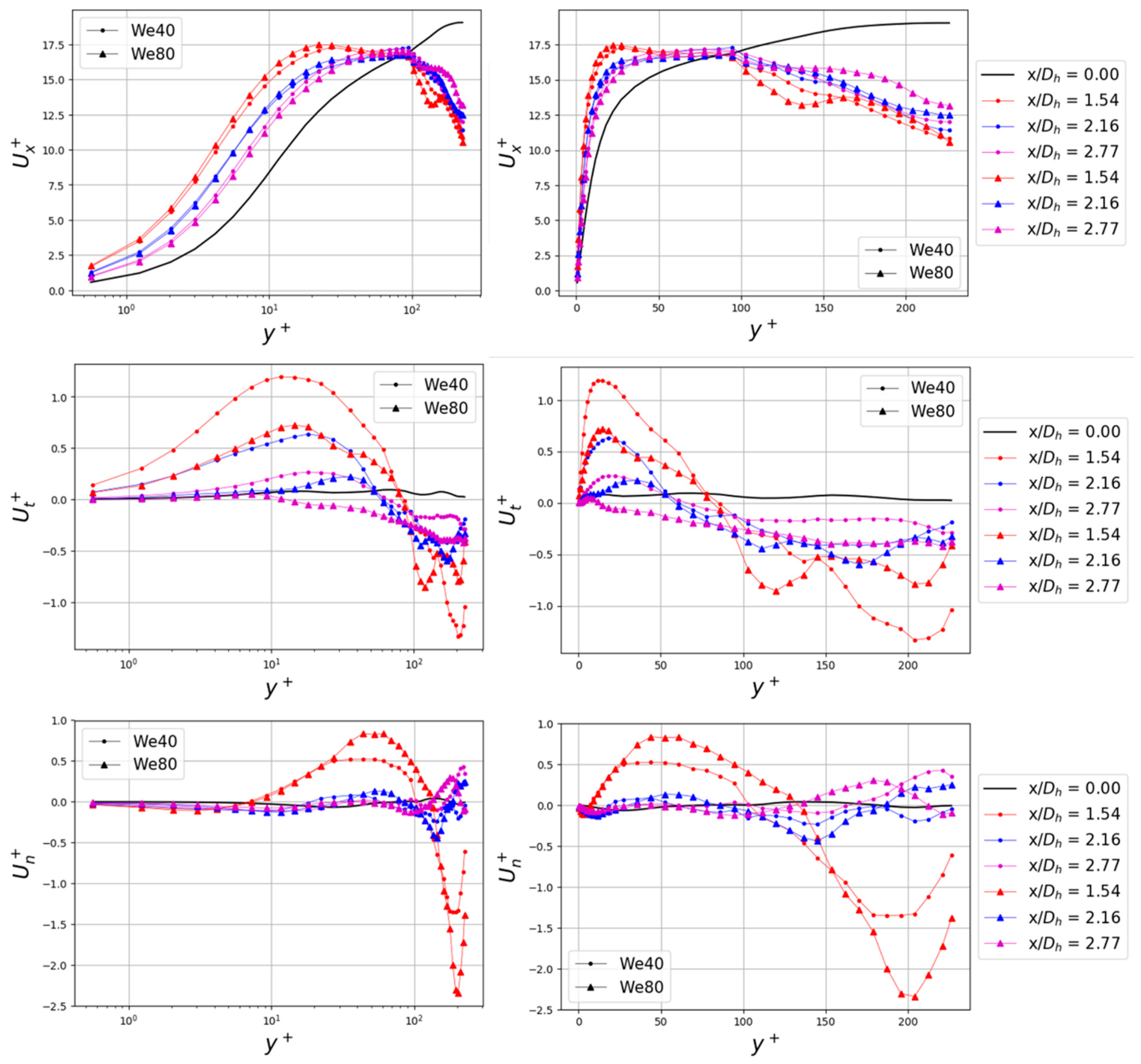
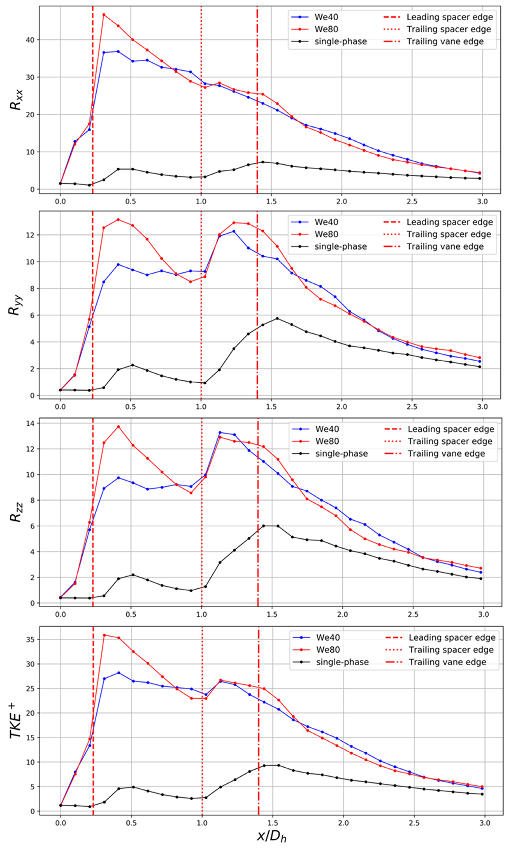
3.1.3. Axial Evolution of Downstream Turbulence

Since the data are collected from the simulations at a high spatial resolution, as displayed in Figure 3, the entire contour map on lateral cross-section can be reconstructed, providing unprecedented insight into the evolution of turbulence flow features in the vicinity of spacer-grid and mixing vane structures. Figure 10 shows the contour maps obtained for the mean normalized streamwise velocity profile for the single and two-phase cases. Note that cubic interpolation is used to generate the contour maps from the point data recorded at probe points, Figure 3. Selected successive downstream planes are shown in Figure 10 (and subsequent figures), starting from the immediate downstream probe plane at x / D h = 1.54 . The wake region is clearly demarcated in the U + profile for the single-phase simulation in the sub-channel center by low mean velocity contours. Also evident is the anti-clockwise swirl imparted to the mean velocity by the mixing vanes. The core wake region, however, rapidly diffuses as we move further downstream, making the mean velocity distribution more uniform laterally. Vestiges of the mixing vane wake and the swirl momentum, nevertheless, are registered at the furthest recorded downstream plane. (The reader is encouraged to refer to the accompanying supplementary material for better visualization of the evolution of all ensuing contour maps.) The presence of droplets in the domain disintegrates the core region and reorganizes the lateral velocity profile. It should be noted that although the contour maps shown in Figure 10 (and subsequent plots) for the two-phase cases are subject to stochasticity due to the random initialization of the droplets, the lateral averaged wall-distance trend for the mean velocity, as shown in Figure 8, closely resembles the single-phase simulation. Further, similar to the single-phase case, the downstream evolution of mean velocity is governed both by lateral diffusion and swirl (see Supplementary Material). Similar trends in contour maps are also observed for the lateral components of normalized mean velocities, V + and W + , included in the Supplementary Material. Figure 11 shows the cross-sectionally averaged normalized mean velocity for all cases, plotted for all axial probe planes. The two-phase cases register a higher, albeit similar, increase in the streamwise velocity at the leading edge of the spacer as compared to the single-phase case. Along the spacer and mixing vane profile, the trend followed by single-phase simulation and both the two-phase cases is similar, including the magnitude of velocity drop near the spacer trailing edge. Further downstream, all cases asymptote to comparable mean velocity, although reduced as compared to average velocity at the inlet cross-section owing to the momentum being transferred to lateral components.
Figure 12, Figure 13 and Figure 14 show the normalized principal Reynolds stress contour maps for all cases. The highest energy for the single-phase simulations is seen in the immediate wake of the mixing vanes, with a starkly identifiable wake region in the subchannel core, which corresponds to Reynolds stress production source. Owing to the dominant effect of dissipation, however, the high Reynolds stress regions in the wake rapidly vanish, restoring a laterally uniform profile (also corroborated by Figure 7). Lateral distribution of the Reynolds stresses in downstream planes is governed by both dissipation and swirl transport (see Supplementary Material). For the two-phase cases, the lateral Reynolds stress distribution at the immediate downstream location ( x / D h = 1.54 ) is stochastic, which may be attributed to limited temporal data available for generating cross-sectional contour maps. It is interesting to note that the highest stresses are not recorded in the sub-channel core, but in the peripheral regions owing to the droplet being pushed towards the periphery by the mixing vanes. Further downstream, the stress distribution is governed by swirl transport and dissipation, similar to single-phase case. Note that, owing to the complex geometrical configuration and presence of droplets, for the two-phase cases, the secondary Reynolds stresses ( R x y , R x z , R y z ) also have a significant magnitude and must be accounted for from a modeling perspective. The plots for the secondary stresses are included in the supplementary material. Observing the laterally averaged profile for the Reynolds stresses, as shown in Figure 15, we can see that the maximum production of stresses is observed at the leading edge of the spacer, followed by significant production, especially for the R y y and R z z components, along the mixing vane profile for all cases. It is interesting to note that all Reynolds stress components (or normalized TKE) for the two-phase cases tend to asymptote to the value of the single-phase at the furthest downstream location.

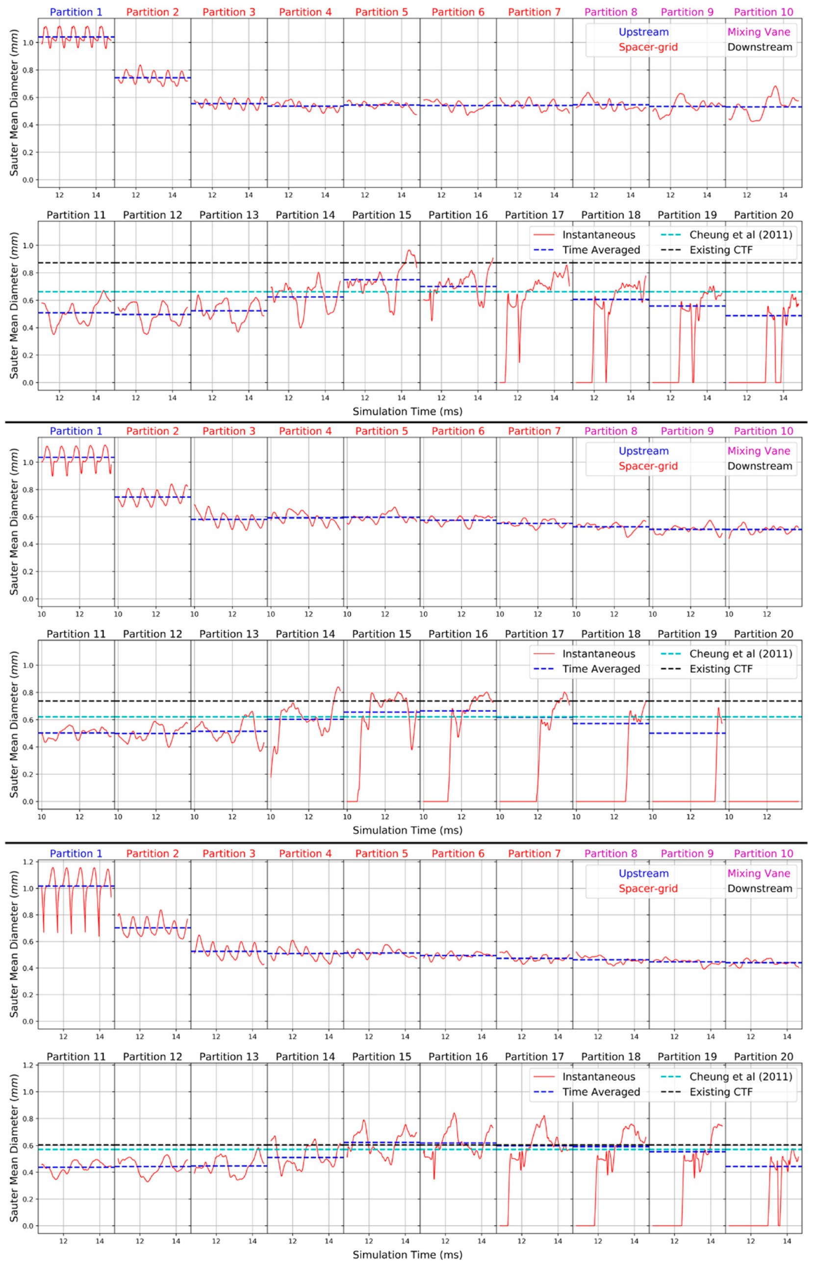
3.2. Axial Evolution of Droplet Sauter Mean Diameter

The droplet dynamics are analyzed for all cases following the method described in [35]. The computational domain is divided into 20 axial regions, and the droplet volume and surface area are integrated and recorded at each time step for each region. The volume and surface area can be evaluated from the LS field, respectively, as,
V p = e Ω e ( 1 H ( ϕ ) ) d Ω
A p = e Ω e H ( ϕ ) n   d Ω
where Ω e represents integration over an element, while the subscript p represents axial partition. Sauter mean diameter for the partitions can then be evaluated as [35],
S M D p = 6 V p A p
The instantaneous and time-averaged evolution of laterally averaged droplet volume is shown in Figure 16 for all cases. The leading edge of the spacer grid resides in Partition 2, while the trailing edge of the mixing vane is in Partition 10. Partitions 11-20 all lie downstream of the internal structures. Fluctuations seen in Partition 1 result from the departure and periodic inception of droplets. Note that the droplets are initialized in batches in Partition 1 (see [35] for details), which results in the periodic oscillation seen in the droplet volume (and surface area and SMD). It should be emphasized that the averaged droplet volume for all three cases is comparable, verifying that the droplets are injected in the domain for all three cases with the same time period. The fluctuations progressively lose their periodicity in the downstream partitions due to changes in morphology and velocity of droplets. Note, however, that the We40 case loses periodicity in fluctuations more rapidly than the We50 or We80 case, which can be attributed to the lower surface tension coefficient for the former case. Due to droplet accumulation at the leading edge of the spacer-grid strap, a sharp increase is seen in the droplet volume and surface area (Figure 17). An increase in the surface area also results in an increase in the relative drag force acting on the deformed or smaller daughter droplets,
F d F g S u r f a c e A r e a V o l u m e 1 S M D
This results in an increased acceleration of the daughter droplets, which manifests as the decreased residence time of droplets in the Partitions further downstream, causing a monotonous decrease in the average droplet volume and surface area. The surface area plot, Figure 17, follows essentially the same trend as the droplet volume. From a modeling perspective, however, the SMD trend, which gives a measure of the droplet morphology, is of greater significance.
Figure 18 shows the instantaneous and time-averaged SMD for all cases. The fluctuations in Partition 1 correspond to the fluctuations observed in droplet volume and surface area. It is, however, interesting to note that the magnitude of fluctuations becomes more pronounced as the Weber number is increased. Re-initialization of the velocity, following Equation (16), in the droplet interior as it is initialized results in a high relative velocity between the droplets and surrounding steam. This causes the droplets to oscillate about the stream-wise axis, and the amplitude of these oscillations increases as the surface tension coefficient is increased, which provides the rationale for the aforementioned observation. The time-averaged SMD trend from Partition 1 to Partition 2 is contrary to what was observed for the volume and surface area, albeit due to the same reason—droplet collision results in an increase in the surface area due to rapid deformation and/or breakup. Along the spacer-grid and mixing vane profile, Partitions 3-10, the time-averaged SMD value remains consistent, close to 0.5, for all cases. In the downstream region, however, beyond Partition 12, the average SMD increases owing to the deformed droplets regaining their sphericity, owing to surface tension force and due to droplet coalescence. Consistent with the observations noted in Figure 2, the relative increase in SMD is more for the We40 case and progressively decreases towards the We80 case. Figure 18 also includes the SMD predictions for each case, obtained from the existing correlation in the STH code CTF (or COBRA-TF) [62] and the proposed correlation by Cheung et al. [17], both based on the upstream collision Weber number, W e c . The time-averaged SMD plots agree well for all cases with the correlation by Cheung et al. in the downstream Partition 15-18. However, as compared to the existing CTF correlation, the average SMD is significantly underpredicted for the We40 case, although the agreement between current results and both correlations progressively improves for cases with higher Weber number.
The time-averaged axial profiles can be discerned more clearly from Figure 19 and Figure 20. It is evident, from the-time averaged droplet volume in Partition 1, that the droplet injection rate at the upstream location of spacer grids is almost equal for all considered cases. An increase in the droplet volume due to collision at the leading edge of the spacer is also comparable for all cases. Following Partition 2, the time-averaged volume monotonously decreases, as noted earlier. Only a slight disruption to this trend is seen near the trailing edge of the mixing vane for the water-steam system cases. It is interesting to note the difference in trends for the same collision Weber number cases, We55-Air and We55, the former being of relatively higher viscosity ratio. The post-collision SMD for the We55-Air case is lower, indicating the droplets undergo more deformation or break up into smaller daughter droplets as compared to We55 case. Further investigation is required to explore the effects of viscosity on droplet dynamics. In Figure 20, only the SMD values obtained from the correlation by Cheung et al. [17] are shown for comparison. Note that increase in the SMD, for all cases, is seen at the same distance downstream from the mixing vane trailing edge (Partition 14, x / D h 2.16 ) . The empirical correlation by Cheung et al. predicts a decrease in the downstream SMD with increasing incident collision Weber number, W e c . Figure 20 corroborates this behavior for the downstream SMD as we move from the We40 to the We80 case for the water–steam system cases. Even considering uncertainty in experimental measurements, uncertainty in the downstream location at which the observations were made and uncertainty and knowledge gaps in the current adiabatic simulations, a good agreement is obtained in the downstream SMD results for all Weber number cases with existing empirical correlation, establishing the viability of large-scale interface capturing methods for analyzing complex PWR flow regimes.

4. Concluding Remarks

The intricate physics constituting two-phase flow in the dispersed flow film boiling (DFFB) regime is either outside the scope of experimental possibility, prohibitively expensive to analyze experimentally or involves measurements rife with uncertainty. This work presents high-fidelity, DNS-scale, interface-capturing simulations with conditions representative of the DFFB regime, enabled by a massively parallel CFD code, PHASTA. The simulations are performed in a typical PWR sub-channel with spacer-grids and mixing vane structures, identified as the dominant structures governing the overall thermal hydraulic feedback of a PWR core in the post-LOCA, DFFB regime. The simulations herein are adiabatic with controlled parameters including the Reynolds number for the continuous phase and the incident collision Weber number for the dispersed phase.
Data are collected from the simulations at a high spatial and temporal resolution, which allows insight into hitherto unexplored turbulence and two-phase statistics. Both single- and two-phase simulations are performed with the same transient inlet flow conditions, allowing a comparison of the evolution of turbulence flow features in the downstream region of the mixing vanes. The mixing vanes provide massive positive feedback to Reynolds stresses, which is further amplified owing to the presence of droplets, registered across the wall-normal coordinate at the immediate downstream location of mixing vanes. Increasing the collision Weber number was also found to increase the energy contained in the streamwise and tangential component towards the sub-channel core; however, the normal Reynolds stress was relatively attenuated. A major source of turbulence production was recorded at the incident face of the spacer-grids and along the mixing vane profile. In the downstream region, the energy contained in all Reynolds stress components rapidly dissipated, with both two-phase and single-phase profiles approaching equivalent asymptote value at the furthest recorded location.
The two-phase simulations also provide data on the droplet volume, surface area and Sauter mean diameter. Droplet collision with spacer-grids and mixing vanes, causing subsequent breakup and/or deformation, results in a sharp increase in surface area. In the DFFB experiments, this manifested as a sharp increase in the heat transfer recorded at the immediate downstream vicinity of the mixing vanes, correlated with the SMD and upstream collision Weber number. Here, we have recorded the instantaneous SMD of the droplets for different Weber numbers in the operating range of DFFB regime and compared the downstream SMD with existing empirical correlations. The data provide insight into the axial evolution of droplet dynamics, and the time-averaged SMD values agree well with empirical correlations.
In comparison to the actual DFFB conditions, there are several factors that contribute to epistemic uncertainty in the quantities of interest presented in this study, viz., the relative change in SMD and continuous phase turbulence at the downstream region. These factors include the lack of heat transfer and phase change modeling, inability to account for quenching and the consequent loss of droplet mass on collision with heated spacers, lack of modeling accounting for Leidenfrost effect witnessed in the experiments and lack of droplet contact angle modeling. In addition, the assumptions of the present study also contribute to aleatoric uncertainty, including monodispersity of incident droplets and their mass flow rate; uncertainty due to numerical discretization and mesh resolution, which will be of significance to droplet breakup events; and uncertainty due to property smearing and mass loss due to re-distancing inherent to the level-set method. A detailed exposition of simulation uncertainties is provided in Saini [43]. Notwithstanding these limitations, the results herein demonstrate the viability of large-scale interface capturing simulations in exploring complex two-phase reactor flow regimes. The high-fidelity data collected from the simulations are archived and intended to be used to guide the development of data-driven and physics-informed turbulence (RANS/LES) and system-thermal hydraulic models.

Supplementary Materials

The following are available online at https://www.mdpi.com/2311-5521/6/2/72/s1. Video We40: Droplet dynamics and flow evolution for We40 case; Video We80: Droplet dynamics and flow evolution for We80 case; Video We40: Droplet dynamics and flow evolution for We40 case; Video U_1ph: Axial evolution of downstream normalized mean streamwise velocity component for single phase case; Video U_We40: Axial evolution of downstream normalized mean streamwise velocity component for We40 case; Video U_We80: Axial evolution of downstream normalized mean streamwise velocity component for We80 case; Video V_1ph: Axial evolution of downstream normalized mean velocity y-component for single phase case; Video V_We40: Axial evolution of downstream normalized mean velocity y-component for We40 case; Video V_We80: Axial evolution of downstream normalized mean velocity y-component for We80 case; Video W_1ph: Axial evolution of downstream normalized mean velocity z-component for single phase case; Video W_We40: Axial evolution of downstream normalized mean velocity z-component for We40 case; Video W_We80: Axial evolution of downstream normalized mean velocity z-component for We80 case; Video Rxx_1ph: Axial evolution of downstream normalized Reynolds stress xx-component for single phase case; Video Rxx_We40: Axial evolution of downstream normalized Reynolds stress xx-component for We40 case; Video Rxx_We80: Axial evolution of downstream normalized Reynolds stress xx-component for We80 case; Video Ryy_1ph: Axial evolution of downstream normalized Reynolds stress yy-component for single phase case; Video Ryy_We40: Axial evolution of downstream normalized Reynolds stress yy-component for We40 case; Video Ryy_We80: Axial evolution of downstream normalized Reynolds stress yy-component for We80 case; Video Rzz_1ph: Axial evolution of downstream normalized Reynolds stress zz-component for single phase case; Video Rzz_We40: Axial evolution of downstream normalized Reynolds stress zz-component for We40 case; Video Rzz_We80: Axial evolution of downstream normalized Reynolds stress zz-component for We80 case; Video Rxy_1ph: Axial evolution of downstream normalized Reynolds stress xy-component for single phase case; Video Rxy_We40: Axial evolution of downstream normalized Reynolds stress xy-component for We40 case; Video Rxy_We80: Axial evolution of downstream normalized Reynolds stress xy-component for We80 case; Video Rxz_1ph: Axial evolution of downstream normalized Reynolds stress xz-component for single phase case; Video Rxz_We40: Axial evolution of downstream normalized Reynolds stress xz-component for We40 case; Video Rxz_We80: Axial evolution of downstream normalized Reynolds stress xz-component for We80 case; Video Ryz_1ph: Axial evolution of downstream normalized Reynolds stress yz-component for single phase case; Video Ryz_We40: Axial evolution of downstream normalized Reynolds stress yz-component for We40 case; Video Ryz_We80: Axial evolution of downstream normalized Reynolds stress yz-component for We80 case

Author Contributions

Conceptualization, N.S. and I.A.B.; methodology, N.S. and I.A.B.; software, N.S. and I.A.B.; validation, N.S.; formal analysis, N.S.; investigation, N.S.; resources, I.A.B.; data curation, N.S.; writing—original draft preparation, N.S.; writing—review and editing, I.A.B.; visualization, N.S.; supervision, I.A.B.; project administration, I.A.B.; funding acquisition, I.A.B. All authors have read and agreed to the published version of the manuscript.

Funding

This research was funded by the Department of Energy’s Nuclear Energy University Program’s Integrated Research Project “Development and Application of a Data-Driven Methodology for Validation of Risk-Informed Safety Margin Characterization Models” in support of the DOE’s LWR Sustainability program’s RISMC R&D Pathway (Project 16-10918).

Data Availability Statement

The data presented in this study are available on request from the corresponding author. The data are not publicly available due to logistical reasons.

Acknowledgments

The simulations presented herein used Acusim linear algebra solution library provided by Altair Engineering Inc. and libraries by Simmetrix Inc. Computing resources under the ASCR Leadership Computing Challenge (ALCC) were used for the simulations.

Conflicts of Interest

The authors declare no conflict of interest.

Appendix A

Figure A1. (Left) Comparison of normalized crosswise Reynolds stress component (Rxn) at the inlet cross-section with DNS data from Lee et al. [52]. (Right) Downstream evolution of Rxn for the two-phase cases (lateral coordinates rotated to t n system).
Fluids 06 00072 g0a1

References

  1. Hochreiter, L.; Cheung, F.; Lin, T.; Baratta, A.; Frepoli, C. Dispersed Flow Heat Transfer under Reflood Conditions in a 49-Rod Bundle: Test Plan and Design—Results from Tasks 1–10; PSU ME/NE-NRC-04-98-041; Pennsylvania State University: State College, PA, USA, 2000. [Google Scholar]
  2. Meholic, M.J. The Development of a Non-Equilibrium Dispersed Flow Film Boiling Heat Transfer Modeling Package. Ph.D. Thesis, The Pennsylvania State University, The Graduate School, College of Engineering, State College, PA, USA, August 2011. [Google Scholar]
  3. Takenaka, N.; Akagawa, K.; Fujii, T.; Nishida, K. Experimental study on flow pattern and heat transfer of inverted annular flow. Nucl. Eng. Des. 1990, 120, 293–300. [Google Scholar] [CrossRef]
  4. Hammouda, N.; Groeneveld, D.; Cheng, S. An experimental study of subcooled film boiling of refrigerants in vertical up-flow. Int. J. Heat Mass Transf. 1996, 39, 3799–3812. [Google Scholar] [CrossRef]
  5. Andreani, M.T.; Yadigaroglu, G. Dispersed Flow Film Boiling; Thermal-Hydraulic Laboratory, Paul Scherrer Institute (PSI): Villigen, Switzerland, 1989. [Google Scholar]
  6. Yoder, G.L.; Rohsenow, W.M. Dispersed Flow Film Boiling; Heat Transfer Laboratory, Department of Mechanical Engineering, Massachusetts Institute of Technology: Cambridge, MA, USA, 1980. [Google Scholar]
  7. Lee, N. PWR FLECHT SEASET Unblocked Bundle, Forced and Gravity Reflood Task Data Evaluation and Analysis Report; No.10; The Commission: Brussels, Belgium, 1982. [Google Scholar]
  8. Bajorek, S.M.; Cheung, F.-B. Rod bundle heat transfer thermal-hydraulic program. Nucl. Technol. 2018, 205, 307–327. [Google Scholar] [CrossRef]
  9. Andreani, M.; Yadigaroglu, G. Difficulties in modeling dispersed-flow film boiling. Heat Mass Transf. 1992, 27, 37–49. [Google Scholar] [CrossRef]
  10. Hochreiter, L. Rod Bundle Heat Transfer Facility: Steady-State Steam Cooling Experiments; United States Nuclear Regulatory Commission, Office of Nuclear Regulatory: Washington, DC, USA, 2014. [Google Scholar]
  11. Riley, M.P. Spacer Grid Induced Heat Transfer Enhancement in a Rod Bundle under Reflood Conditions; Pennsylvania State University: State College, PA, USA, 2014. [Google Scholar]
  12. Miller, D.J.; Cheung, F.; Bajorek, S. Investigation of grid-enhanced two-phase convective heat transfer in the dispersed flow film boiling regime. Nucl. Eng. Des. 2013, 265, 35–44. [Google Scholar] [CrossRef]
  13. Riley, M.; Mohanta, L.; Cheung, F.; Bajorek, S.; Tien, K.; Hoxie, C. Experimental studies of spacer grid thermal hydraulics in the dispersed flow film boiling regime. Nucl. Technol. 2015, 190, 336–344. [Google Scholar] [CrossRef]
  14. Yao, S.C.; Hochreiter, L.E.; Leech, W.J. Heat-Transfer Augmentation in Rod Bundles Near Grid Spacers. J. Heat Transf. 1982, 104, 76–81. [Google Scholar] [CrossRef]
  15. Avramova, M. Development of an Innovative Spacer Grid Model Utilizing Computational Fluid Dynamics within a Sub-Channel Analysis Tool; Pennsylvania State University: State College, PA, USA, 2007. [Google Scholar]
  16. Hochreiter, L.; Cheung, F.; Lin, T.; Frepoli, C.; Sridharan, A.; Todd, D.; Rosal, E.R. Rod Bundle Heat Transfer Test Facility Test Plan and Design; NUREG CR-6975; US Nuclear Regulatory Commission: Washington, DC, USA, 2010. [Google Scholar]
  17. Cheung, F.; Bajorek, S. Dynamics of droplet breakup through a grid spacer in a rod bundle. Nucl. Eng. Des. 2011, 241, 236–244. [Google Scholar] [CrossRef]
  18. Wachters, L.; Smulders, L.; Vermeulen, J.; Kleiweg, H. The heat transfer from a hot wall to impinging mist droplets in the spheroidal state. Chem. Eng. Sci. 1966, 21, 1231–1238. [Google Scholar] [CrossRef]
  19. Senda, J. Experimental Studies on the Behavior of a Small Droplet Impinging upon a Hot Surface. In Proceedings of the ICLASS-82, Madison, WI, USA, 20–24 June 1982. [Google Scholar]
  20. Behzadi, A.; Issa, R.; Rusche, H. Modelling of dispersed bubble and droplet flow at high phase fractions. Chem. Eng. Sci. 2004, 59, 759–770. [Google Scholar] [CrossRef]
  21. Gosman, A.D.; Lekakou, C.; Politis, S.; Issa, R.I.; Looney, M.K. Multidimensional modeling of turbulent two-phase flows in stirred vessels. AIChE J. 1992, 38, 1946–1956. [Google Scholar] [CrossRef]
  22. Lance, M.; Bataille, J. Turbulence in the liquid phase of a uniform bubbly air–water flow. J. Fluid Mech. 1991, 222, 95. [Google Scholar] [CrossRef]
  23. Wang, S.K.; Lee, S.J.; Jones, O.C.; Lahey, R.T. 3-D turbulence structure and phase distribution measurements in bubbly two-phase flows. Int. J. Multiph. Flow 1987, 13, 327–343. [Google Scholar] [CrossRef]
  24. Lee, S.L.; Lahey, R.T.; Jones, O.C. The Prediction of Two-Phase Turbulence and Phase Distribution Phenomena Using a K-κ Model. Jpn. J. Multiph. Flow 1989, 3, 335–368. [Google Scholar] [CrossRef]
  25. Rusche, H. Computational Fluid Dynamics of Dispersed Two-Phase Flows at High Phase Fractions. Ph.D. Thesis, Imperial College London, University of London, London, UK, 2002. [Google Scholar]
  26. Balachandar, S.; Eaton, J.K. Turbulent Dispersed Multiphase Flow. Annu. Rev. Fluid Mech. 2010, 42, 111–133. [Google Scholar] [CrossRef]
  27. Rzehak, R.; Krepper, E. CFD modeling of bubble-induced turbulence. Int. J. Multiph. Flow 2013, 55, 138–155. [Google Scholar] [CrossRef]
  28. Rasquin, M.; Smith, C.; Chitale, K.; Seol, E.S.; Matthews, B.A.; Martin, J.L.; Sahni, O.; Loy, R.M.; Shephard, M.S.; Jansen, K.E. Scalable Implicit Flow Solver for Realistic Wing Simulations with Flow Control. Comput. Sci. Eng. 2014, 16, 13–21. [Google Scholar] [CrossRef]
  29. Bolotnov, I.A. Phasta-NCSU Git Repository. Available online: https://github.com/PHASTA/phasta-ncsu (accessed on 1 December 2020).
  30. Nagrath, S.; Jansen, K.E.; Lahey, R.T. Computation of incompressible bubble dynamics with a stabilized finite element level set method. Comput. Methods Appl. Mech. Eng. 2005, 194, 4565–4587. [Google Scholar] [CrossRef]
  31. Fang, J.; Mishra, A.V.; Bolotnov, I.A. Interface Tracking Simulation of Two-phase Bubbly Flow in A PWR Subchannel. In Proceedings of the International Embedded Topical Meeting on Advances in Thermal Hydraulics—2014, American Nuclear Society 2014 Annual Meeting (ATH ‘14), Reno, NV, USA, 15–19 June 2014. [Google Scholar]
  32. Bolotnov, I.A.; Jansen, K.E.; Drew, D.A.; Oberai, A.A.; Lahey, R.T.; Podowski, M.Z. Detached direct numerical simulations of turbulent two-phase bubbly channel flow. Int. J. Multiph. Flow 2011, 37, 647–659. [Google Scholar] [CrossRef]
  33. Fang, J.; Cambareri, J.; Li, M.; Saini, N.; Bolotnov, I.A. Interface-Resolved Simulations of Reactor Flows. Nucl. Technol. 2020, 206, 133–149. [Google Scholar] [CrossRef]
  34. Zimmer, M.D.; Bolotnov, I.A. Slug-to-churn vertical two-phase flow regime transition study using an interface tracking approach. Int. J. Multiph. Flow 2019, 115, 196–206. [Google Scholar] [CrossRef] [Green Version]
  35. Saini, N.; Bolotnov, I.A. Interface capturing simulations of droplet interaction with spacer grids under DFFB condi-tions. Nucl. Eng. Des. 2020, 364, 110685. [Google Scholar] [CrossRef]
  36. Lu, J.; Biswas, S.; Tryggvason, G. A DNS study of laminar bubbly flows in a vertical channel. Int. J. Multiph. Flow 2006, 32, 643–660. [Google Scholar] [CrossRef]
  37. Santarelli, C.; Fröhlich, J. Direct Numerical Simulations of spherical bubbles in vertical turbulent channel flow. Influence of bubble size and bidispersity. Int. J. Multiph. Flow 2016, 81, 27–45. [Google Scholar] [CrossRef]
  38. Chang, C.-W.; Dinh, N. Classification of machine learning frameworks for data-driven thermal fluid models. Int. J. Therm. Sci. 2019, 135, 559–579. [Google Scholar] [CrossRef] [Green Version]
  39. Ma, T.; Santarelli, C.; Ziegenhein, T.; Lucas, D.; Fröhlich, J. Direct numerical simulation–based Reynolds-averaged closure for bubble-induced turbulence. Phys. Rev. Fluids 2017, 2, 034301. [Google Scholar] [CrossRef]
  40. Ling, J.; Kurzawski, A.; Templeton, J. Reynolds averaged turbulence modelling using deep neural networks with embedded invariance. J. Fluid Mech. 2016, 807, 155–166. [Google Scholar] [CrossRef]
  41. Liu, Y.; Dinh, N.; Sato, Y.; Niceno, B. Data-driven modeling for boiling heat transfer: Using deep neural networks and high-fidelity simulation results. Appl. Therm. Eng. 2018, 144, 305–320. [Google Scholar] [CrossRef] [Green Version]
  42. Bao, H.; Feng, J.; Dinh, N.; Zhang, H. Computationally efficient CFD prediction of bubbly flow using physics-guided deep learning. Int. J. Multiph. Flow 2020, 131, 103378. [Google Scholar] [CrossRef]
  43. Saini, N. High-fidelity Interface Capturing Simulations of the Post-LOCA Dispersed Flow Film Boiling Regime in a Pres-Surized Water Reactor Sub-Channel. Ph.D. Thesis, North Carolina State University, Raleigh, NC, USA, 2020. [Google Scholar]
  44. Whiting, C.H.; Jansen, K.E. A stabilized finite element method for the incompressible Navier-Stokes equations using a hierarchical basis. Int. J. Numer. Methods Fluids 2001, 35, 93–116. [Google Scholar] [CrossRef]
  45. Ibanez, D.A.; Seol, E.S.; Smith, C.W.; Shephard, M.S. PUMI: Parallel unstructured mesh infrastructure. ACM Trans. Math. Softw. (TOMS) 2016, 42, 17. [Google Scholar] [CrossRef]
  46. Sahni, O.; Carothers, C.D.; Shephard, M.S.; Jansen, K.E. Strong Scaling Analysis of a Parallel, Unstructured, Implicit Solver and the Influence of the Operating System Interference. Sci. Program. 2009, 17, 261–274. [Google Scholar] [CrossRef] [Green Version]
  47. Sussman, M.; Smereka, P.; Osher, S. A Level Set Approach for Computing Solutions to Incompressible Two-Phase Flow. J. Comput. Phys. 1994, 114, 146–159. [Google Scholar] [CrossRef]
  48. Nagrath, S.; Jansen, K.E.; Lahey, R.T. Three Dimensional Simulation of Incompressible Two-Phase Flows Using a Stabilized Finite Element Method and a Level Set Approach; Preprint; Elsevier Science: Amsterdam, The Netherlands, 2003. [Google Scholar]
  49. Brackbill, J.U.; Kothe, D.B.; Zemach, C. A continuum method for modeling surface tension. J. Comput. Phys. 1992, 100, 335–354. [Google Scholar] [CrossRef]
  50. Fatemi, E.; Sussman, M. An efficient interface preserving Level-Set Re-distancing algorithm and its application to interfacial incompressible fluid flow. SIAM J. Sci. Statist. Comput. 1995, 158, 36. [Google Scholar]
  51. Chen, N.H. An Explicit Equation for Friction Factor in Pipe. Ind. Eng. Chem. Fundam. 1979, 18, 296–297. [Google Scholar] [CrossRef]
  52. Lee, M.; Moser, R.D. Direct numerical simulation of turbulent channel flow up to Re_tau 5200″. J. Fluid Mech. 2015, 774, 395–415. [Google Scholar] [CrossRef]
  53. Thomas, A.M.; Fang, J.; Bolotnov, I.A. Estimation of shear-induced lift force in laminar and turbulent flows. In Proceedings of the International Topical Meeting on Advances in Thermal Hydraulics—2014 (ATH ′14), Reno, NV, USA, 15–19 June 2014. [Google Scholar]
  54. Busco, G.; Merzari, E.; Hassan, Y.A. Invariant analysis of the Reynolds stress tensor for a nuclear fuel assembly with spacer grid and split type vanes. Int. J. Heat Fluid Flow 2019, 77, 144–156. [Google Scholar] [CrossRef]
  55. Wierzba, A. Deformation and breakup of liquid drops in a gas stream at nearly critical Weber numbers. Exp. Fluids 1990, 9, 59–64. [Google Scholar] [CrossRef]
  56. Jin, Y.; Miller, D.J.; Qiao, S.; Rau, A.; Kim, S.; Cheung, F.-B.; Bajorek, S.M.; Tien, K.; Hoxie, C.L. Uncertainty analysis on droplet size measurement in dispersed flow film boiling regime during reflood using image processing technique. Nucl. Eng. Des. 2018, 326, 202–219. [Google Scholar] [CrossRef]
  57. Papka, M.; Coghlan, S.; Isaacs, E.; Peters, M.; Messina, P. Mira: Argonne’s 10-Petaflops Supercomputer; Argonne National Laboratory (ANL): Argonne, IL, USA, 2013. [Google Scholar]
  58. Gottfried, B.; Lee, C.; Bell, K. The leidenfrost phenomenon: Film boiling of liquid droplets on a flat plate. Int. J. Heat Mass Transf. 1966, 9, 1167–1188. [Google Scholar] [CrossRef]
  59. Pope, S.B. Turbulent Flows; Cambridge University Press: Cambridge, UK, 2001. [Google Scholar]
  60. Fang, J.; Rasquin, M.; Bolotnov, I.A. Interface tracking simulations of bubbly flows in PWR relevant geometries. Nucl. Eng. Des. 2017, 312, 205–213. [Google Scholar] [CrossRef] [Green Version]
  61. Nagib, H.M.; Chauhan, K.A. Variations of von Kármán coefficient in canonical flows. Phys. Fluids 2008, 20, 101518. [Google Scholar] [CrossRef]
  62. Avramova, M.N.; Salko, R.K. CTF Theory Manual; Technical Report for the Office of Scientific and Technical Information: Oak Ridge, TN, USA, 2016. [Google Scholar] [CrossRef]
Figure 1. Pressurized water reactors (PWR) sub-channel geometry with spacer-grids and mixing vanes (left). Tetrahedral mesh, 367.5 M elements, with extended boundary layers on mixing vane surfaces also shown (right). Inlet cross-section located at x = 0.
Fluids 06 00072 g001
Figure 2. Instantaneous state of droplets and velocity contours for the We40 (top) and We80 (bottom) case at t = 14.75 and 13.35 ms, respectively. Note that gravitational body force acts along the negative x coordinate.
Fluids 06 00072 g002
Figure 3. Probe configuration for data collection on a plane. The probes are organized into 20 loci in each quadrant, yielding a homogeneous distribution. All planes, along axial length, shown on right, totaling 84,908 probes.
Fluids 06 00072 g003
Figure 4. Comparison of mean normalized streamwise velocity profile at the inlet cross-section with direct numerical simulation (DNS) data from Lee et al. [52] and Fang et al. [60].
Fluids 06 00072 g004
Figure 5. Comparison of mean Reynolds stress and turbulent kinetic energy (TKE) profile at the inlet cross-section with DNS data from Lee et al. [52] and Fang et al. [60] (lateral coordinates rotated to t n system).
Fluids 06 00072 g005
Figure 6. Comparison of downstream normalized mean velocity components for the We80 case with the single-phase simulation. Inlet profile (similar for both cases) is shown in solid black. Profile at three downstream planes are shown for each case (lateral coordinates rotated to t n system).
Fluids 06 00072 g006
Figure 7. Comparison of downstream normalized Reynolds stress components for the We80 case with the single-phase simulation. Inlet profile (similar for both cases) is shown in solid black. Profiles at three downstream planes are shown for each case (lateral coordinates rotated to t n system).
Fluids 06 00072 g007
Figure 8. Comparison of normalized mean velocity components for the We40 and We80 cases. Profiles at three downstream probe planes are shown (lateral coordinates rotated to t n ).
Fluids 06 00072 g008
Figure 9. Comparison of normalized principal Reynolds stress component profile for the We40 and We80 cases. Profiles at three downstream probe planes are shown (lateral coordinates are rotated to t n ).
Fluids 06 00072 g009
Figure 10. Axial evolution of downstream normalized mean streamwise velocity for the single-phase (left), We40 (middle) and We80 (right) cases.
Fluids 06 00072 g010
Figure 11. Axial evolution of plane averaged normalized mean streamwise velocity profile for the single-phase, We40 and We80 cases.
Fluids 06 00072 g011
Figure 12. Axial evolution of downstream normalized streamwise component of Reynolds stress for the single-phase (left), We40 (middle) and We80 (right) cases.
Fluids 06 00072 g012
Figure 13. Axial evolution of downstream normalized lateral (y) component of Reynolds stress for the single-phase (left), We40 (middle) and We80 (right) cases.
Fluids 06 00072 g013
Figure 14. Axial evolution of downstream normalized lateral (z) component of Reynolds stress for the single-phase (left), We40 (middle) and We80 (right) cases.
Fluids 06 00072 g014
Figure 15. Axial evolution of plane averaged normalized Reynolds stress components and turbulent kinetic energy profile for the single-phase, We40 and We80 cases.
Fluids 06 00072 g015
Figure 16. Axial evolution of total droplet volume in partitions for We40, We55 and We80 (topbottom) water–steam system cases.
Fluids 06 00072 g016
Figure 17. Axial evolution of total surface area in partitions for We40, We55 and We80 (topbottom) water–steam system cases.
Fluids 06 00072 g017
Figure 18. Axial evolution of Sauter mean diameter (SMD) in partitions for We40, We55 and We80 (topbottom) water–steam system cases. For each case, the SMD value obtained from existing empirical correlations is also shown.
Fluids 06 00072 g018
Figure 19. Axial profile of time-averaged droplet volume (left) and surface area (right) in domain partitions for all two-phase cases.
Fluids 06 00072 g019
Figure 20. Axial profile of time-averaged SMD in domain partitions for all two-phase cases. The values obtained with the RBHT (rod bundle heat transfer) correlation by Cheung et al. [17] are also annotated.
Fluids 06 00072 g020
Table 1. Properties for representative dispersed flow film boiling (DFFB) regime simulations.
PropertiesSingle PhaseWe55-Air
(Saini et al. [35])
Properties @ 30 Psi, Steam Superheat 100 K
We40We55We80
Density ratio ( ρ l / ρ g ) ρ g = 1.185   kg / m 3 10001029.59
Viscosity ratio ( μ l / μ g ) μ g = 9.1 × 10 6   Pa · s 4813.49
Bulk Reynolds number, R e b 11,822
Friction Reynolds number, R e τ 242.539
Mean inlet gas velocity, U   ( m / s ) 7.0
Collision Weber number, W e c (Equation (14))-55405580
Aerodynamic Weber number, W e a (Equation (17))-0.3190.2530.3480.507
Injected absolute droplet velocity, u d   ( m / s ) 2.051.97
Injected droplet diameter, D   ( mm ) -1.0
Injected droplet Reynolds number, R e d = ρ g u r e l D / μ g 643.71654.67
Surface tension coefficient, σ   ( N / m ) -0.0910.1180.0860.059
Gravity, g   ( m / s 2 ) −9.81
Publisher’s Note: MDPI stays neutral with regard to jurisdictional claims in published maps and institutional affiliations.

