Abstract
Bora is a strong or severe, relatively cold, gusty wind that usually blows from the northastern quadrant at the east coast of the Adriatic Sea. In this study bora’s turbulence triplet covariances were analysed, for the first time, for bora flows. The measurements used were obtained from the measuring tower on Pometeno brdo (“Swept-Away Hill”), in the hinterland of the city of Split, Croatia. From April 2010 until June 2011 three components of wind speed and sonic temperature were measured. The measurements were performed on three heights, 10, 22 and 40 m above the ground with the sampling frequency of 5 Hz. During the observed period, total of 60 bora episodes were isolated. We analyse the terms in prognostic equations for turbulence variances. In that respect, the viscous dissipation term was calculated using two approaches: (i) inertial dissipation method (εIDM) and (ii) direct approach from the prognostic equations for variances of turbulence (εEQ). We determine that the direct approach can successfully reproduce the shape of the curve, but the values are for several orders of magnitudes smaller compared to the real data. Further, linear relationship between εIDM and εEQ was obtained. Using the results for εEQ, viscous dissipation rate in longitudinal, transversal and vertical direction was determined. It is shown that viscous dissipation has the greatest impact on bora’s longitudinal direction. The focus is on the turbulence transport term, i.e., the triplet covariance term. For the first time, it is found that turbulence transport is very significant for the intensity of near−surface bora flows. Furthermore, turbulence transport can be both positive and negative, yet intensive. It is mostly negative at the upper levels and positive at the lower levels. Therefore, turbulence transport, in most cases, takes away turbulence variance from the upper levels and brings it down to the lower ones. This is one of the main findings of this study; it adds to the understanding of peculiarities of bora wind, and perhaps some other severe winds.
1. Introduction
Strong-to-severe, relatively cold, very gusty wind that usually blows from the northeastern quadrant at the east coast of the Adriatic Sea (and many other dynamically similar places around the world) is known as bora. Bora is synoptically caused by collapsing of a relatively cold northeastern air mass across the Dinaric Mountains—a mountain barrier perpendicular to the air flow [1,2,3,4,5] which generates steep, large amplitude mountain waves (mesoscale part of the flow setup). As a result, the flow characteristics are strongly influenced by complex, presumably steep terrain, i.e., maximum wind speeds are reached at places where the flow direction is predominantly perpendicular to the mountain barrier and near major gaps in orography (e.g., [3,6,7]).
During severe bora events, which lead to severe downslope windstorms, collapsing of air mass over a mountainous barrier usually occurs in a hydraulic flow regime, which allows the wind to accelerate on both the ascending and descending sides, thereby significantly increasing the speed of the oncoming flow [3,6,8,9]. Hence, bora generally achieves a wide range of wind speeds with gusts; the bora wind gusts of more than 60 m s−1 often occur (e.g., [6,10,11]). For such mostly violent circumstances, Lepri et al. 2014 and 2017 [12,13] show that layers of bora flows are well mixed and predominantly near−neutrally stratified with typical values of the stability parameter ζ (defined as the ratio of height above the ground and the Obukhov length) settled roughly between −0.2 and 0.2.
To date, Bora’s macroscale and mesoscale characteristics have been excessively studied (e.g., [4,9,14,15,16,17,18,19]), while its microscale characteristics have not yet been fully resolved. Thus, during the last two decades or so, the main emphasis in bora research has focused on its microscale characteristics. This includes phenomena as gust pulsations [18,20], lee−wave rotors (e.g., [5,9]), turbulence dissipation rates [21] and along−coast bora properties and their sensitivity to different atmospheric boundary−layer parametrisation schemes [7]. Likewise, engineering aspects of the bora flows are still not settled (e.g., [12,13,22,23]). Babić et al. [24] isolated 17 strong winter bora events from 1 January to 31 March 2011 to study the vertical profiles of the turbulence fluxes. The expected behaviour of turbulent fluxes is determined for medium horizontal wind speeds, up to 12 m s−1. However, for wind speeds greater than 12 m s−1, significant vertical divergences in the profiles of vertical momentum fluxes were observed. Namely, the fluxes were larger at the 22 m, than 10 m and 40 m level. This hints the aim of this study.
Overall, it cannot be overstressed that bora wind generally does not belong to standard wind types. One of these reasons is already stated in [24] and mentioned here, while the others pertain to turbulence length scales associated with lateral and vertical velocity fluctuations which are much larger than the values recommended in international standards for the respective terrain type [13,22]. Kozmar and Grisogono [23] elaborated on that in the light of the fact that bora belongs to severe downslope windstorms; therefore, the standard approaches to model wind turbine control systems and gain scheduling design (e.g., [25]) generally do not apply to severe bora wind. To add a point, severe bora, that may reach hurricane speeds (e.g., [6]), stops all the traffic in the area where it blows and it becomes unusable for wind energy harvesting, sometimes for several days or even a few weeks.
This paper continues on the study of bora’s microscale features, more precisely, turbulence triplet covariances (the third-order turbulence moments) will be assessed. The main motivation for this work are significant divergences of turbulent fluxes (second-order turbulence moments) from Babić et al. [24]. Considering bora’s turbulence anisotropy, the terms of longitudinal and transversal components of the prognostic equation for turbulence variances will be assessed with the emphasis on turbulence transport term—the triplet covariance term. We hypothesise that turbulence transport is responsible for a reasonable maintenance of Kolmogorov’s isotropic turbulence in bora flows, characterised by large mean velocity gradients (e.g., [26,27]). Additionally, the challenge here will be to address the viscous dissipation terms in the prognostic equations for turbulence variances.
This study expects to give a further insight into the bora turbulence processes. The very structure of the paper is as follows: Section 2 briefly outlines theoretical review and methods; Section 3 gives details about the data used; the results are presented in Section 4, and conclusions are given in Section 5.
2. Theoretical Background
Since bora is mostly a turbulent flow of the corresponding downslope windstorm, we start with suitable Reynolds averaged prognostic equation for turbulence variances. This equation contains the subjects of this study—the turbulence triplet covariances term.
2.1. Prognostic Equations for Turbulence Variances
Prognostic equation for turbulence variances, i.e., twice turbulence kinetic energy (TKE), without introducing any special assumption is given by (e.g., [28]):
where Einstein’s summation convention is used and the terms respectively represent: I local change of the variance, II advection of the variance by the mean wind, III buoyancy term of production or loss, IV mechanical production, V turbulence transport (redistribution), VI transport of the variance by the pressure perturbations and VII viscous dissipation. All variables in Equation (1) have their standard meaning: Ui and u’i are the mean and perturbation parts of velocity in the xi direction, respectively, Θv and θ’v are the mean and perturbation part of the virtual potential temperature, p’ is the perturbation part of the atmospheric pressure, ρ is the mean air density, and υ is the kinematic molecular viscosity of the air.
I II III IV V VI VII
Detailed description of each individual term is given in e.g., [28]. Moreover, by introducing the standard horizontal homogeneity assumption in Equation (1), and by considering that the pressure measurements were not performed, (1) becomes:
where W is the mean vertical wind speed component and R represents the residual term (sum of the pressure redistribution term and the terms with horizontal derivatives).
Within the scope of this paper the main focus is on the turbulence transport term as this term contains a triplet covariance; it describes how the variance (and hence the components of turbulence kinetic energy) is moved around by turbulent eddies . Before that, a detailed analysis of the viscous dissipation term will be demonstrated.
2.2. Viscous Dissipation
Viscous dissipation rate (VD) is responsible for destruction of turbulent eddies, i.e., it always causes a decrease in the variance with time. VD is defined as (with the horizontal homogeneity assumption introduced):
where ν is the kinematic molecular viscosity of the air, 1.5 × 10⁻⁵ m2 s−1 (e.g., [29]). Hence, VD is defined as the sum of the dissipation in longitudinal, transversal and vertical direction (). To determine VD directly from Equation (3), extremely high−frequency spatio−temporal measurements are required. Since that kind of measurements usually are not available, VD is obtained using the standard inertial dissipation method (IDM) applied to streamwise wind speed component:
where Su(f) stands for Fourier spectrum of the streamwise wind speed component and Kolmogorov similarity and Taylor’s hypothesis are assumed (e.g., [7]). The value for the constant αu is taken to be 0.53, which is broadly used in the scientific community in general, as well as for the bora flows [7,11,21,30,31].
Considering bora’s turbulence anisotropy, each individual component of Equation (2) is analysed; hence, each component of VD needs to be assessed. However, using IDM, only the total VD from the TKE budget equation can be determined. Thereby, IDM is not adequate, as such, for assessment of VD components. Moreover, note that by IDM one can assess the total VD from (1); VD without introducing any special assumptions such as horizontal homogeneity. Here, the components of VD were reconstructed directly from Equation (3), even though extremely high−frequency measurements were not available.
3. Data and Methods
The data used were obtained from the measuring tower on Pometeno brdo (“Swept-Away Hill”, 43° 36′ N, 16° 28′ E), nearby Dugopolje, in the hinterland of the second largest city in Croatia, Split (Figure 1). The hill itself is oriented in the north−west to south−east direction of the Dinaric Alps, thereby it is perpendicular to the mean direction of the bora flow. The three−level measuring tower was located at the top of Pometeno brdo (approximately 620 m above mean sea level, ASL in m) and was surrounded by the complex heterogeneous terrain. A detailed description of the measuring site and surrounding orography is given in Babić et al. [24].
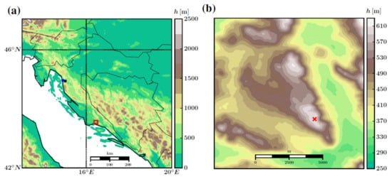
Figure 1.
(a) Map of Croatia and a part of the Adriatic Sea. The square in (a) marks in the area (b) around the location of Pometeno Brdo (Swept−Away Hill); the cross in (b) shows the meteorological tower position. The colour bars denote height ASL in m. The other marks in (a) show the location of the town of Senj (NW from (b)), famous for bora severe wind, and Vratnik Pass, respectively. (Reprinted from ref. [24]).
The measuring tower with three “WindMaster Pro” ultrasonic anemometers (manufactured by Gill Instruments Limited, Lymington, UK) was active from April 2010 until June 2011. During the observed period, three wind speed components, as well as sonic temperature, were measured. Measurements were performed with the sampling frequency of 5 Hz at the three levels, 10, 22 and 40 m above the ground level, AGL. The data were collected using a CR1000 datalogger (manufactured by Campbell Scientific, Inc., Logan, Utah, USA). To reduce distortion influences from the tower, anemometers were mounted at the end of 2 m long aluminium booms. Moreover, the booms were pointed toward the north−east to fully capture the entire span of bora directions [24].
Quality check of the dataset included the removal of all questionable and erroneous outliers [32]. Since our aim is the spectral analysis of data, all missing data points were linearly interpolated. Such data points were statistically insignificant, they were less than 5% of total data points.
Bora episodes are defined as follows: (i) 10 min averages of wind direction have to be in the northeastern quadrant (from 25° to 85°), (ii) duration of the flow has to be at least 10 h and (iii) 10 min averages of wind speed on mid−level, 25 m, has to be ≥5 m s−1 (e.g., [13]). Based on these criteria, a total of 60 bora episodes were isolated with the cumulative duration of 2064 h. The shortest bora episode lasted 11 h and the longest 127 h. Mean wind speeds (10 min averages) at 10 m of all bora episodes ranged from 5 m s−1 to 12.4 m s−1 while the strongest gusts reached 40.9 m s−1. This overall statistic indicates the dedication of the study considered since bora windstorm is a sort of Croatian natural brand.
The analysis of bora’s turbulence characteristics was performed in a streamwise coordinate system, with the vertical axis parallel to the force of gravity. Hence, the coordinate system was rotated in such a way that the new x−axis aligns with the direction of the mean wind at 25 m mid−level which was obtained by linearly interpolating wind speeds between 10 and 40 m. It should be noted that every bora episode was shortened to the whole number of 30 min intervals.
4. Results
4.1. Averaging Time Scales
In order to determine the turbulent perturbations, a suitable averaging time scale must be obtained. Thus, the weighted power spectral densities of all three wind speed components for all observed bora episodes were calculated. To compute power spectral densities, Welch’s method [33] has been used with a window of 217 data points. The overlapping of the windows was set to 50% and obtained spectra were further smoothed by block averaging (e.g., [34]).
Finally, a composite spectrum of all 60 bora episodes was obtained. Medians of weighted spectra are shown in Figure 2. Weighted spectra, fS(f), are very suitable for the analysis because the area under the spectral curve represents the variance of the analysed variable, i.e., the energy of the wind in our case. A spectral minimum in the weighted spectra of u and v components is obvious; however, it is not possible to observe a clear minimum in spectra of w component. This is because w component spectra do not contain large amount of energy at larger, i.e., synoptic scales since bora flows are driven by cyclonic, anticyclonic or frontal systems, where horizontal motions are predominant. Therefore, w component spectra for bora flows do not exhibit a maximum on the left side of the spectrum (e.g., [24]). Nevertheless, based on our u and v spectra, it is estimated that the spectral gap is around the period of T 15 min. Although this estimate is somewhat subjective and based on the visualisation of the spectrum, it is accepted within the scope of this paper as it also agrees with the other results on the topic of bora’s turbulence on Pometeno brdo (e.g., [13,24]). Moreover, we decided not to expand a spectral gap scale further (e.g., to a value of 30 min, which is a kind of standard in the literature) because we want to avoid possible contamination of turbulence by the sub−mesoscale features, whose presence is clearly evident in our v wind speed component spectrum (indicated by the pronounced peak in the spectrum on scales between 15 and 30 min).
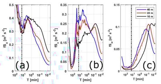
Figure 2.
Composite frequency−weighted power spectral densities (medians shown) of the (a) longitudinal (u), (b) transversal (v) and (c) vertical (w) wind speed components for all three measurement heights of all bora episodes. Vertical dashed line marks 15 min period.
Having a suitable averaging time scale obtained, turbulent perturbations of all three components of wind speed and sonic temperature (u′, v′, w′, T′) were determined using Reynolds’s decomposition; moving average of 15 min was used to calculate perturbations and then the time series of obtained perturbations were divided in 30 min blocks. Further analysis is based on the assessment of the time series of the terms in Equation (2). Individual terms are averaged over 30 min. Time series of the terms are defined at the three mid−levels, 16 m (between 10 and 22 m), 25 m (mid−level between 10 and 40 m) and 31 m (between 22 and 40 m). A more detailed analysis was conducted on the viscous dissipation term and will be given in the next three subsections. After that, the analysis of the other terms in Equation (2) is given.
4.2. Determination of Viscous Dissipation
The VD term from Equation (2) was obtained using the IDM (4) which, so far, many times has been proven to work for bora flows [7,11,21,31]. It needs to be said that 5 Hz sampling rate is probably too low to resolve the inertial subrange in our signals. However, many authors have showed that the −5/3 slope can extend even outside of the inertial subrange towards the lower frequencies and this feature can then be used for the estimation of ε using the IDM (e.g., [35,36,37]). Log−log representation of medians of our spectra of the longitudinal wind speed component calculated for all 30 min intervals involved in the analysis also show this extension of the −5/3 slope towards the lower frequencies (which agrees with previous studies for bora flows made by Večenaj et al., 2010 [21], 2011 [30], 2012 [7], Večenaj 2012 [31] and Šoljan et al. 2018 [11]), with the frequency band closest to the −5/3 slope settled roughly between 0.45 and 1 Hz (not shown). Therefore, we are confident in the estimation of ε applying the IDM to our 30 min data blocks.
However, values obtained using the IDM represent the total VD in the 1D TKE budget equation, while in this work we will need its components from Equation (2). For this purpose, we use the formulation of VD obtained directly from the prognostic equations for turbulence variances (Equation (3)). We are aware that our measurements with 5 Hz sampling frequency are limited, and that we probably cannot expect that applying Equation (3) to our data can result with physically well−justified result. However, in the absence of better tools, and with the aim to determine the components that contribute to ε, we apply Equation (3) to our data, expecting that the obtained result should be empirically correlated with ε provided by the IDM. The results of these two time series for the longest bora episode are given in Figure 3. It is clear that obtained curves have the same shape, but their values differ for a few or even several orders of magnitude. Hence, the direct approach successfully reproduces the variability of VD, but the values are much lower than those obtained by IDM. The analysis of all the other bora episodes yields similar results. The main reason for the VD underestimation via Equation (3) is excessively large (≥10 m, instead of ~O (1 cm) for this approach since Equation (3) implies ; furthermore, unavailability of the corresponding horizontal contributions to such also adds to this VD underestimation. Nevertheless, the overall qualitative agreement in terms of the shape of estimated VD via two approaches and the corresponding correlation coefficients is appealing, suggesting that there might be something physically relevant between the two, rather than that such high correlation obtained on large data set being just a mere coincidence. However, an in−depth analysis of the potentially relevant physical relationship does not fall within the scope of this paper, and is definitely a subject for some future work.
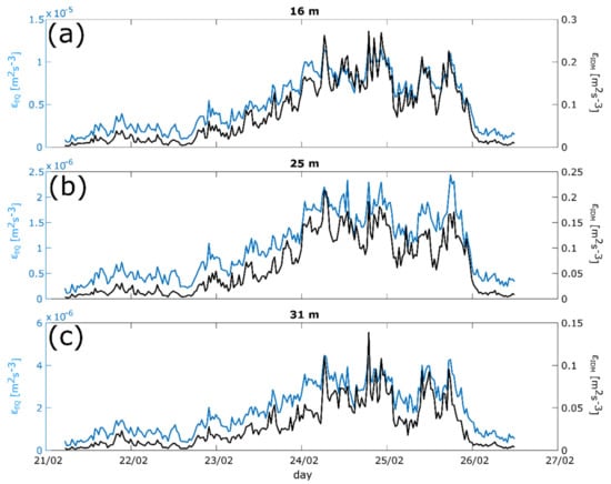
Figure 3.
Time series of viscous dissipation, VD, obtained directly from prognostic equation for turbulence variances (left, light curve) and VD obtained by IDM method (right, black) for the longest bora episode threat (a) 16 m, (b) 25 m and (c) 31 m mid−levels. The square of the correlation coefficients are at 16 and 25 m and at 31 m mid−levels.
Since the direct approach showed the ability to reproduce the shape of the VD curve obtained by IDM, linear regression using the least squares method between the two analysed approaches was performed, y = ax + b, where x corresponds to the VD obtained directly () and y corresponds to the VD estimated by IDM (). Linear regression was performed on the whole data set, for all bora episodes and for all 30 min intervals (Figure 4). The intercept y term has values close to zero and the slope term is height dependent. Moreover, the deviation from the straight line obtained is smaller in the area close to the origin and dispersion of values increases towards larger VD’s. Thus, we expect linear regression to be most successful for relatively small values of VD. The highest values of VD are expected for the longest and strongest bora episodes. In the observed data set, the relatively weaker episodes are more numerous than the stronger and severe ones, which is why most values are grouped around the starting point.
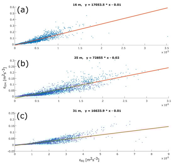
Figure 4.
Linear regression between VD obtained by IDM () and by direct approach ( ) for all bora episodes and at (a) 16 m, (b) 25 m and (c) 31 m mid−levels. The intercept y and the slope term are given in the title.
Considering the regression coefficients obtained, VD determined by linear regression is:
where coefficients a and b have the values shown in Figure 4. The results for the longest bora episode are given in Figure 5. The deviations between and are the smallest for relatively weak VD; by increasing the dissipation values, the deviations increase as well. It is also clear that does not reproduce the maximum values of appropriately. This might be due to the fact that the relationship between and is not quite linear as we assumed, but based on the scatter plots shown in Figure 4, it is hard to presume anything else beyond the linear relationship between the two. Furthermore, is in some cases negative, which is not physically justified; VD is the ultimate destruction of TKE and should always represent a negative term in Equation (2). Hence, is always positive and with the minus sign in Equation (2) always corresponds to the destruction of turbulence energy. The same is not true for which apparently takes negative values at the beginning and the end of each bora episode; in those cases, the corresponding values are small, and with negative b coefficient becomes spuriously negative.
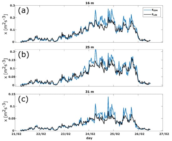
Figure 5.
Time series of VD obtained by linear regression (light curve) and VD obtained by IDM (black) for the longest bora episode and at (a) 16 m, (b) 25 m and (c) 31 m mid−levels. The square of the correlation coefficients are at 16 and 25 m and at 31 m mid−levels.
Although high−frequency measurements in space and time are required for the calculation of VD by the direct approach, it has been demonstrated that the discussed approach successfully reproduces the shape of the curve of VD obtained by IDM. Hence, this approach is chosen to assess VD in the longitudinal, transversal and vertical direction.
As was noted before, VD obtained using the IDM method is the sum of viscous dissipation rate in x, y, and z directions () which occur in the individual components of Equation (2). Using IDM, we estimate the total VD but not the distribution of VD by components. Thereby, IDM is not adequate for the analysis of the individual members in Equation (2). On the other hand, the direct approach can estimate each component of viscous dissipation (); however, the results obtained are for several orders of magnitude smaller than the expected values.
As the direct approach proved to be unsuccessful in reproducing the exact value of VD but successful in reproducing the shape of the dissipation curve, the results of the direct approach were used to determine mutual relationship between and . After determining the relationship between the individual components, the results obtained by IDM were used to determine the value of and .
Thus, the ratios between each component obtained with the direct approach ( and ) and were determined. The ratios were calculated for all 30 min intervals of all bora episodes and for every mid−level, Table 1. As expected, the longitudinal component carries the largest (71%) and the vertical component the smallest (4%) proportion of the total VD for bora flows.

Table 1.
Means of the ratios between VD components and its total. The ratios are calculated for all bora episodes and all mid−levels.
Lastly, was multiplied by the obtained ratios and the time series of each component of VD were obtained. The time series for the longest bora episode are shown together with the time series of the other terms in Equation (2) in Figure 6.
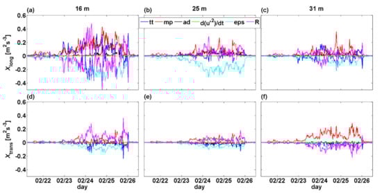
Figure 6.
Time series of all the terms in Equation (2) at all three mid−levels: (a,d) 16 m, (b,e) 25 m, (c,f) 31 m for the longest bora episode. For every mid−level, the upper subplot (a–c) shows longitudinal and the lower (d–f) transversal terms. The terms are marked as follows: turbulence transport—black, mechanical production—red, advection of the variance by the mean wind—dark blue, local rate of change of the variance—green, VD—light blue, and the residual term—grey.
Finally, the estimation of VD components enables the analysis of the terms in the prognostic equation for turbulence variances (2) which will be conducted in the following subsections. The main focus of the analysis will be on turbulence transport term—the triplet covariance term.
4.3. Time Series of the Terms in the Prognostic Equation for Turbulence Variances
Time series of the terms in Equation (2) were obtained for all bora episodes; results for the longest bora episode are in Figure 6. It is important to notice that we analysed only longitudinal and transversal components in Equation (2) as the terms in the vertical component are at least for an order of magnitude smaller than the horizontal ones (not shown).
Generally, all the terms have greater values at lower levels and in the longitudinal direction. Further, it is evident that the dominant terms are the mechanical production term (MP), VD and the residual term, in agreement with the previous research [38,39]. Moreover, the values of the turbulent transport (TT) term are comparable to, or even greater in absolute values, than the generally dominant terms. It is important to point out that TT can be both positive and negative while the sign changes occur particularly at 16 m mid−level. On the other hand, the vertical advection of the variance with the mean wind and the local change of the variance are negligible. It is interesting to notice that TT and the residual term are always of opposite signs and that TT follows the changes of the residual member (the sum of all terms that cannot be determined directly).
4.4. Relationship between Turbulent Transport and Mechanical Production Term
The relationship between TT and dominant terms, namely, the relationship between MP and TT, has also been studied. The first and obvious reason for choosing MP is that it is one of the dominant terms, and the second reason is that, typically, this term is always positive. Once again, the buoyancy term is insignificant for strong bora flows [11,13]. The ratios between TT and MP (Figure 7) were assessed for all bora episodes (and therefore, all 30 min intervals) at all analysed mid−levels and for both components of Equation (2). As MP is always positive, a positive ratio indicates positive TT and vice versa, a negative ratio indicates negative TT.
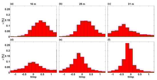
Figure 7.
Histograms of the ratios between turbulence transport and mechanical production terms obtained for: (a,d) 16 m, (b,e) 25 m and (c,f) 31 m mid−levels. For every mid−level, the upper histograms, (a–c), refer to the longitudinal, and the lower histograms, (d–f), to the transversal direction. Medians are given in Table 2.
TT in the x-direction is mostly positive at the mid−level of 16 and 25 m, while it is mostly negative at the mid−level of 31 m. The associated median values are given in Table 2. On the other hand, TT in the y-direction is mostly negative at all mid−levels, although there are cases in which TT might take a different sign from the one described here. Moreover, it is important to notice that in some cases TT receives values that are comparable to or even greater than MP. That adds up to our hypothesis that strong bora turbulence tends to remain nearly isotropic in the Kolmogorov’s inertial subrange due to TT terms which try to smooth out the large gradients among mean wind components. We guess that the fully complete TT terms are largely responsible for the qualitative agreement between IDM and Equation (3), where Equation (3) is missing: (i) finer , and (ii) horizontal contributions that can be large in bora flows due to excessive gradients among mean wind speed components (e.g., [16,23,26,40]). According to the relationships of TT and MP terms, our results might be comparable to some other studies, but the absolute values of these terms obtained in this paper belong to among the highest values reported in the existing literature (e.g., [30,40,41,42]).
Table 2.
Medians of the ratios between the turbulence transport and mechanical production term. Ratios are calculated for all bora episodes and mid−levels.
Furthermore, a positive TT indicates that the variance is transported to the observed level; conversely, a negative TT indicates that the variance is transported from the observed level (i.e., TKE is taken away by the negative TT). Thus, to sum up, the x component of the variance is in most cases transported from higher to lower levels; this is one of the main results of this study. This is in qualitative accordance with Klemp and Durran [4], Belušić et al. [18], Grisogono and Belušić [6], Večenaj et al. [7] and Kozmar and Grisogono [23] who explained that the bora shooting flow, i.e., bora strong low−level jet, is the key dynamical ingredient for bora’s severity and gustiness.
5. Conclusions
Data collected from the measuring tower on the top of Pometeno brdo (“Swept-Away Hill”), in the hinterland of Split, Croatia were used to estimate turbulence triplet covariances for bora flows. During the measuring period, a total of 60 bora episodes were extracted. To study bora’s turbulence properties, a time averaging scale was required—using spectral analysis, it is determined that time averaging scale is about 15 min.
The main objective of this paper was to analyse, for the first time, turbulence triplet covariances for bora flows. For this purpose, the members of the prognostic equation for turbulence variances (twice TKE) are estimated. Viscous dissipation, VD, is determined using two approaches: (i) standard inertial dissipation method, IDM, and (ii) using direct approach from the prognostic equations for turbulence variances. Although the direct approach requires measurements with much greater spatial and temporal frequency than those available here, it has proven successful in a way that it reproduces reasonably well the shape of the curve of VD estimated by IDM. However, the values obtained by the direct approach are a few or several orders of magnitude smaller than those obtained by IDM. Using the results obtained by the direct approach, VD in the longitudinal, transverse, and vertical directions of the bora flow was estimated. It was shown that VD has the greatest impact in the longitudinal direction.
Furthermore, special emphasis was placed on the analysis of the turbulence transport term, the term which contains turbulence triplet covariance. It is shown that turbulent transport is significant for intensity of the bora flows and acts differently at different elevations; the estimation of this term was one of the main goals of this study. It is shown that turbulent transport may take on both positive and negative values within heights ≈ 10 m; in the longitudinal direction, it is mostly negative at higher levels and positive at lower levels. In other words, turbulent transport takes away turbulence variance from higher levels (where the bora shooting flow occurs) and brings it down to the lower ones. This is one of the main findings of this work and it adds to the understanding of peculiarities of bora wind near the surface, especially its gustiness. Almost needless to say, engineering standards for such flows usually do not account for such types of gustiness (e.g., [13,23]).
Author Contributions
Conceptualization, Ž.V.; methodology, Ž.V.; software, B.M.; validation, Ž.V., B.M. and B.G.; formal analysis, B.M.; investigation, Ž.V., B.M. and B.G.; resources, Ž.V., B.M. and B.G.; data curation, Ž.V.; writing—original draft preparation, Ž.V. and B.M.; writing—review and editing, B.G.; visualization, B.M.; supervision, Ž.V. and B.G.; project administration, Ž.V. and B.G.; funding acquisition, Ž.V. and B.G. All authors have read and agreed to the published version of the manuscript.
Funding
This research was partialy enabled by SWALDRIC (IZHRZO−180587) project, which is financed within the Croatian−Swiss Research Program of the Croatian Science Foundation and the Swiss National Science Foundation with funds obtained from the Swiss−Croatian Cooperation Programme. In addition, Croatian Science Foundation HRZZ−IP−2016−06−2017 (WESLO) support is also gratefully acknowledged.
Institutional Review Board Statement
Not applicable.
Informed Consent Statement
Not applicable.
Data Availability Statement
Not applicable.
Conflicts of Interest
The authors declare no conflict of interest.
References
- Mohorovičić, A. Interessante Wolkenbildung űber der Bucht von Buccari (with a comment from the editor J. Hann). Meteorol. Z. 1889, 24, 56–58. [Google Scholar]
- Jurčec, V. On mesoscale characteristics of bora conditions in Yugoslavia. Pure Appl. Geophys. 1981, 119, 215–227. [Google Scholar]
- Smith, R.B. Aerial observation of the Yugoslavian bora. J. Atmos. Sci. 1987, 44, 269–297. [Google Scholar] [CrossRef]
- Klemp, J.; Durran, D. Numerical modelling of bora winds. Meteorol. Atmos. Phys. 1987, 36, 215–227. [Google Scholar] [CrossRef]
- Grubišić, V.; Orlić, M. Early observations of rotor clouds by Andrija Mohorovičić. Bull. Amer. Meteorol. Soc. 2007, 88, 693–700. [Google Scholar] [CrossRef]
- Grisogono, B.; Belušić, D. A review of recent advances in understanding the meso− and micro−scale properties of the severe Bora wind. Tellus A 2009, 61, 1–16. [Google Scholar] [CrossRef]
- Večenaj, Ž.; Belušić, D.; Grubišić, V.; Grisogono, B. Along coast features of the bora related turbulence. Bound. Layer Meteorol. 2012, 143, 527–545. [Google Scholar] [CrossRef]
- Bajić, A. Application of the two−layer hydraulic theory on the severe northem Adriatic bora. Meteorol. Rundsch. 1991, 44, 129–133. [Google Scholar]
- Gohm, A.; Mayr, G.J.; Fix, A.; Giez, A. On the onset of bora and the formation of rotors and jumps near a mountain gap. Q. J. R. Meteorol. Soc. 2008, 134, 21–46. [Google Scholar] [CrossRef]
- Belušić, D.; Klaić, Z.B. Mesoscale dynamics, structure and predictability of a severe Adriatic bora case. Meteorol. Z. 2006, 15, 157–168. [Google Scholar] [CrossRef]
- Šoljan, V.; Belušić, A.; Šarović, K.; Nimac, I.; Brzaj, S.; Suhin, J.; Belavić, M.; Večenaj, Ž.; Grisogono, B. Micro−scale properties of different bora types. Atmosphere 2018, 9, 116–141. [Google Scholar] [CrossRef]
- Lepri, P.; Kozmar, H.; Večenaj, Ž.; Grisogono, B. A summertime near−ground velocity profile of the bora wind. Wind Struc. 2014, 19, 505–522. [Google Scholar] [CrossRef]
- Lepri, P.; Večenaj, Ž.; Kozmar, H.; Grisogono, B. Bora wind characteristics for engineering applications. Wind Struc. 2017, 24, 596–611. [Google Scholar]
- Enger, L.; Grisogono, B. The response of bora−type flow to sea surface temperature. Q. J. R. Meteorol. Soc. 1998, 124, 1227–1244. [Google Scholar] [CrossRef]
- Klaić, Z.B.; Belušić, D.; Grubišić, V.; Gabela, L.; Ćoso, L. Mesoscale airflow structure over the northern Croatian coast during MAP IOP 15—A major bora event. Geofizika 2003, 20, 23–61. [Google Scholar]
- Grubišić, V. Bora−driven potential vorticity banners over the Adriatic. Q. J. R. Meteorol. Soc. 2004, 130, 2571–2603. [Google Scholar] [CrossRef]
- Jiang, Q.F.; Doyle, J.D. Wave breaking induced surface wakes and jets observed during a bora event. Geophys. Res. Let. 2005, 32, L17807. [Google Scholar] [CrossRef]
- Belušić, D.; Žagar, M.; Grisogono, B. Numerical simulation of pulsations in the bora wind. Q. J. R. Meteorol. Soc. 2007, 133, 1371–1388. [Google Scholar] [CrossRef]
- Horvath, K.; Ivatek−Šahdan, S.; Ivančan−Picek, B.; Grubišić, V. Evolution and structure of two severe cyclonic bora events: Contrast between the northern and southern Adriatic. Weather Forecast 2009, 24, 946–964. [Google Scholar] [CrossRef]
- Belušić, D.; Pasarić, M.; Orlić, M. Quasi−periodic Bora gusts related to the structure of the troposphere. Q. J. R. Meteorol. Soc. 2004, 130, 1103–1121. [Google Scholar] [CrossRef]
- Večenaj, Ž.; Belušić, D.; Grisogono, B. Characteristics of the near−surface turbulence during a bora event. Ann. Geophys. 2010, 28, 155–163. [Google Scholar] [CrossRef]
- Lepri, P.; Večenaj, Ž.; Kozmar, H.; Grisogono, B. Near−ground turbulence of the bora wind in summertime. J. Wind Eng. Ind. Aerodyn. 2015, 147, 345–357. [Google Scholar] [CrossRef]
- Kozmar, H.; Grisogono, B. Characteristics of Downslope Wind Storms in the View of the Typical Atmospheric Boundary Layer. In The Oxford Handbook of Non−Synoptic Wind Storms; Hangan, H., Kareem, A., Eds.; Oxford University Press: Oxford, UK, 2021; Chapter in press. [Google Scholar] [CrossRef]
- Babić, N.; Večenaj, Ž.; Kozmar, H.; Horvath, K.; Grisogono, B. On turbulent fluxes during strong winter bora events. Bound. Layer Meteorol. 2016, 158, 331–350. [Google Scholar] [CrossRef]
- Bianchi, F.D.; De Battista, H.; Mantz, R.J. Wind Turbine Control Systems: Principles, Modelling and Gain Scheduling Design; Springer: London, UK, 2007; Volume 19. [Google Scholar]
- Kuzmić, M.; Grisogono, B.; Li, X.M.; Lehner, S. Examining deep and shallow Adriatic bora events. Q. J. R. Meteol. Soc. 2015, 141, 3434–3438. [Google Scholar] [CrossRef]
- Freire, L.S. Critical flux Richardson number for Kolmogorov turbulence enabled by TKE transport. Q. J. R. Meteorol. Soc. 2019, 145, 1551–1558. [Google Scholar] [CrossRef]
- Stull, R.B. An Introduction to Boundary Layer Meteorology; Kluwer Academic Publishers: Dordrecht, The Netherlands, 1988; p. 666. [Google Scholar]
- Piper, M.; Lundquist, J.K. Surface layer turbulence measurements during a frontal passage. J. Atmos. Sci. 2004, 61, 1768–1780. [Google Scholar] [CrossRef]
- Večenaj, Ž.; De Wekker, S.F.J.; Grubišić, V. Near surface characteristics of the turbulence structure during a mountain wave event. J. Appl. Meteor. Climat. 2011, 50, 1088–1106. [Google Scholar] [CrossRef]
- Večenaj, Ž. Characteristics of the Bora Related Turbulence. Ph.D. Thesis, University of Zagreb, Zagreb, Croatia, 2012; p. 83. [Google Scholar]
- Vickers, D.; Mahrt, L. Quality control and flux sampling problems for tower and aircraft data. J. Atmos. Ocean. Technol. 1997, 14, 512–526. [Google Scholar] [CrossRef]
- Welch, P.D. The use of Fast Fourier Transform for the estimation of power spectra: A method based on time averaging over short, modified periodograms. In IEEE Transactions on Audio and Electroacoustics; IEEE: Piscataway, NJ, USA, 1967; Volume 15, pp. 70–73. [Google Scholar]
- Kaimal, J.C.; Finnigan, J.J. Atmospheric Boundary Layer Flows. Their Structure and Measurement; Oxford University Press: Oxford, UK, 1994; p. 304. [Google Scholar]
- Champagne, F.H. The finescale structure of the turbulent velocity field. J. Fluid. Mech. 1978, 86, 67–108. [Google Scholar] [CrossRef]
- Mestayer, P.G. Local isotropy and anisotropy in a high−Reynolds−number turbulent boundary layer. J. Fluid. Mech. 1982, 125, 475–503. [Google Scholar] [CrossRef]
- Babić, N. The Analysis of Bora’s Turbulent Fluxes in the Hinterland of Split, Croatia. Ph.D. Thesis, University of Zagreb, Zagreb, Croatia, 2013; p. 52. [Google Scholar]
- Babić, N.; Večenaj, Ž.; Horvath, K.; Grisogono, B. Evaluation of vertical eddy fluxes divergence for multiple bora events. In Proceedings of the ICAM 2013—International Conference on Alpine Meteorology, Kranjska Gora, Slovenia, 3–7 June 2013. [Google Scholar]
- Kuzmić, M.; Li, X.M.; Grisogono, B.; Tomažić, I.; Lehner, S. TerraSAR−X observations of the northeastern Adriatic bora: Early results. Acta Adriat. 2013, 54, 13–26. [Google Scholar]
- Moeng, C.H.; Sullivan, P.P. A comparison of shear−and buoyancy−driven planetary boundary layer flows. J. Atmos. Sci. 1994, 51, 999–1022. [Google Scholar] [CrossRef]
- Dwyer, M.J.; Patton, E.G.; Shaw, R.H. Turbulent kinetic energy budgets from a large−eddy simulation of airflow above and within a forest canopy. Bound. Layer Meteorol. 1997, 84, 23–43. [Google Scholar] [CrossRef]
- Srivastava, M.K.; Sarthi, P.P. Turbulent kinetic energy in the atmospheric surface layer during the summer monsoon. Meteorol. App. 2002, 9, 239–246. [Google Scholar] [CrossRef]


Publisher’s Note: MDPI stays neutral with regard to jurisdictional claims in published maps and institutional affiliations. |
© 2021 by the authors. Licensee MDPI, Basel, Switzerland. This article is an open access article distributed under the terms and conditions of the Creative Commons Attribution (CC BY) license (https://creativecommons.org/licenses/by/4.0/).