Large Eddy Simulation of Hypersonic Turbulent Boundary Layers

Abstract

The recent revival of interest in developing new hypersonic vehicles brings attention to the need for accurate prediction of hypersonic flows by computational methods. One of the challenges is prediction of aerothermodynamic loading over the surface of the vehicles. Reynolds Average Navier-Stokes (RANS) methods have not shown consistent accuracy in prediction of such flows. Therefore, new methods including Large Eddy Simulations (LES) should be investigated. In this paper, the LES method is used for prediction of the boundary layer over a flat plate. A new recycling-rescaling method is tested. The method uses total enthalpy and static pressure along with the velocity components to produce the best results for the Law of the Wall, turbulent statistics and turbulent Prandtl number.

1. Introduction

There is a recent revival of interest in developing hypersonic vehicles. Examples includes Boeing Hypersonic Airliner [1], SpaceLiner [2], and LAPCAT A2 [3]. This recent interest focuses attention on several fields in hypersonic flow physics including prediction of aerothermodynamic loading over the vehicle’s surface. There is no consistently accurate prediction of aerothermodynamic loading over the entire body of a vehicle. One example of the problematic prediction of aerothermodynamic loading is the prediction in the regions with shock wave boundary layer interactions. The inaccurate prediction of aerothermodynamic loading in the regions of shock wave boundary layer interactions can result in disastrous failure in the structure of the vehicle [4,5].

Reynolds Average Navier-Stokes (RANS) methods have not shown consistent accuracy in prediction of aerothermodynamic loading in the shock wave boundary layer interaction regions in hypersonic flows [6]. As an example, Kumar et al. [7] use different RANS models to predict the flowfield over a hollow cylinder flare at Mach 9.6. The RANS models include Spalart-Allmaras (SA) RC-QCR2013, SST, Goldberg-Rt, $k-ϵ$-Rt, SA-Catris, and SA-Neg turbulent models. Their results show a significant change in prediction of the separation region size from no separation to a very large separation region.

An alternate computational method is Large Eddy Simulation (LES). It is proven that LES can provide accurate prediction of shock wave boundary layer interaction in supersonic flows. Examples are Loginov et al. [8], Touber and Sandham [9], Morgan et al. [10], Ritos et al. [11], Ritos et al. [12], and Hadjadj [13]. However, LES is rarely used for prediction of hypersonic shock wave boundary layer interactions. Examples of the usage of LES in hypersonic shock wave boundary layer interactions are discussed below.

Edwards et al. [14] performed a Wall Modeled LES (hybrid RANS/LES) of a shock wave boundary layer interaction over a compression ramp at Mach 5 with $T_{\mathrm{w}}/T_{\mathrm{a}\mathrm{w}}=1.0$, where $T_{\mathrm{w}}$ is wall temperature and $T_{\mathrm{a}\mathrm{w}}$ is the adiabatic wall temperature. The RANS model uses the SST turbulent model of Menter [15]. In general, their results are in reasonable agreement with the experimental data. However, the plateau pressure in the separated region is underestimated and the pressure recovery downstream of the interaction region is overestimated.

Fang et al. [16] performed an LES of a hypersonic flow past a single fin at Mach 5 and $T_{\mathrm{w}}/T_{\mathrm{a}\mathrm{w}}=1.0$ for fin and $T_{\mathrm{w}}/T_{\mathrm{a}\mathrm{w}}=0.81$ for the plate. The subgrid scale stresses and heat transfer are modeled by the dynamic Smagorinsky model [17,18]. The instantaneous time-dependent inflow condition is generated by a separate LES simulation using a wall blowing and suction technique. The inflow condition shows a good agreement with the Law of the Wall and incompressible and low speed compressible density scaled turbulent fluctuations. The surface pressure over the fin is in agreement with the experimental data; however, the peak skin friction coefficient in the vicinity of the first reattachment point is underpredicted by a factor of four.

Fu et al. [19] performed a Wall Modeled LES of a hypersonic turbulent flow past two parallel fins at Mach 8.23. The inflow condition upstream of the leading edge of the flat plate over which two sharp fins are installed is generated as uniform flow with turbulent fluctuations created by a synthetic turbulence method. The subgrid scale stresses are modeled by a static coefficient Vreman model. The LES results are in general agreement with experimental normalized mean surface pressure and mean heat transfer over the flat plate and fins.

One possible explanation for the rarity of LES applications in hypersonic flows is the existence of cold walls in hypersonic experiments. The existence of a cold wall makes it difficult to create a model to generate the instantaneous time-dependent inflow condition in the boundary layer. To generate the inflow condition, five variables are needed to be recycled for the inflow condition, namely, three components of velocity and two state parameters. One method was introduced by Sheng Xu and Pino Martin [20] in which the boundary layer is divided into three sections namely, viscous sublayer, logarithmic region, and outer layer. In their model, each of these three sections is modeled separately and then blended together using three weighting functions.

The objective of this paper is to evaluate a new recycling-rescaling method for generation of the instantaneous time-dependent inflow boundary layer to be used in hypersonic turbulent LES. The new method recycles total enthalpy and static pressure in addition to the three components of velocity. This new method does not assume a constant pressure inside the boundary layer. The new recycling-rescaling method is compared to the more traditional ways that assume constant pressure in the boundary layer and recycles the three components of velocity and generates the inflow temperature either using Walz’s equation [21] or recycling the mean temperature. The new recycling-rescaling method is tested for different wall temperatures and using different grids. This method will enable researchers to create a dynamic inflow condition to be used for solving hypersonic turbulent shock wave boundary layer interactions with a cold wall.

2. Materials and Methods

2.1. Governing Equations

The compressible Large Eddy Simulation governing equations are obtained by spacial filtering of the time-dependent compressible Navier-Stokes equations. The Favre averaging is the common spatial averaging used for this purpose. The Favre averaging of an arbitrary variable $\mathcal{F}(x_i,t)$ is defined as

$$\tilde{\mathcal{F}}=\frac{\overline{\rho \mathcal{F}}}{\overline{\rho }},$$

(1)

where $\overline{\rho }$ is the mean density. Therefore, the instantaneous expression of an arbitrary variable $\mathcal{F}$ is

$$\mathcal{F}(x_i,t)=\tilde{\mathcal{F}}+{\mathcal{F}}^{″}.$$

(2)

The conventional spatial average of a variable $\mathcal{G}(x_i,t)$ is denoted $\overline{\mathcal{G}}$ and thus

$$\mathcal{G}(x_i,t)=\overline{\mathcal{G}}+{\mathcal{G}}^{\prime }.$$

(3)

The Favre-averaged governing equations for a perfect gas are

$$\begin{array}{ccc}\hfill \frac{\partial \overline{\rho }}{\partial t}+\frac{\partial \overline{\rho }{\tilde{u}}_i}{\partial x_i}& =& 0,\hfill \end{array}$$

(4)

$$\begin{array}{ccc}\hfill \frac{\partial \overline{\rho }{\tilde{u}}_i}{\partial t}+\frac{\partial \overline{\rho }{\tilde{u}}_i{\tilde{u}}_j}{\partial x_j}& =& -\frac{\partial \overline{p}}{\partial x_i}+\frac{\partial {\mathcal{T}}_{ij}}{\partial x_j},\hfill \end{array}$$

(5)

$$\begin{array}{ccc}\hfill \frac{\partial \overline{\rho }\tilde{e}}{\partial t}+\frac{\partial }{\partial x_j}\left(\overline{\rho }\tilde{e}+\overline{p}\right){\tilde{u}}_j& =& \frac{\partial {\mathcal{H}}_j}{\partial x_j},\hfill \end{array}$$

(6)

$$\begin{array}{ccc}\hfill \overline{p}& =& \overline{\rho }R\tilde{T},\hfill \end{array}$$

(7)

where $\widetilde{u_i}$ are the Favre-averaged velocity components in the Cartesian coordinates, $x_i$ are the Cartesian coordinates ($i=1,2,3$), $\overline{p}$ is the average pressure, ${\mathcal{T}}_{ij}$ is the total stress, ${\mathcal{H}}_j$ is the energy flux (due to heat transfer and work done by the total stress), and $\tilde{e}$ is the Favre-averaged total energy per unit mass

$$\overline{\rho }\tilde{e}=\overline{\rho }{c}_v\tilde{T}+\frac{1}{2}\overline{\rho }{\tilde{u}}_i{\tilde{u}}_i+\overline{\rho }k,$$

(8)

where $\overline{\rho }k$ is the subgrid scale turbulence kinetic energy per unit volume

$$\overline{\rho }k=\frac{1}{2}\overline{\rho }\left(\widetilde{u_i{u}_i}-{\tilde{u}}_i{\tilde{u}}_i\right).$$

(9)

The total stress is

$${\mathcal{T}}_{ij}={\tau }_{ij}+{\overline{\sigma }}_{ij},$$

(10)

where ${\tau }_{ij}$ is the subgrid scale stress tensor

$${\tau }_{ij}=-\overline{\rho }\left(\widetilde{u_i{u}_j}-{\tilde{u}}_i{\tilde{u}}_j\right),$$

(11)

and therefore ${\tau }_{ii}=-2\overline{\rho }k$. The molecular viscous stress tensor ${\overline{\sigma }}_{ij}$ can be approximated as [18]

$${\overline{\sigma }}_{ij}=\mu \left(\tilde{T}\right)\left(-\frac{2}{3}\frac{\partial {\tilde{u}}_k}{\partial x_k}{\delta }_{ij}+\frac{\partial {\tilde{u}}_i}{\partial x_j}+\frac{\partial {\tilde{u}}_j}{\partial x_i}\right),$$

(12)

where $\mu \left(\tilde{T}\right)$ is the molecular viscosity based on the Favre-averaged static temperature $\tilde{T}$.

The energy flux ${\mathcal{H}}_j$ is

$${\mathcal{H}}_j={\mathcal{Q}}_j+{\mathcal{T}}_{ij}{\tilde{u}}_i,$$

(13)

where the total heat transfer ${\mathcal{Q}}_j$ is

$${\mathcal{Q}}_j=Q_j+{\overline{q}}_j.$$

(14)

The subgrid scale heat flux $Q_j$ is

$$Q_j=-c_p\overline{\rho }\left(\widetilde{u_{j}T}-{\tilde{u}}_j\tilde{T}\right),$$

(15)

and ${\overline{q}}_j$ is the molecular heat flux

$${\overline{q}}_j=\kappa \left(\tilde{T}\right)\frac{\partial \tilde{T}}{\partial x_j},$$

(16)

where $\kappa \left(\tilde{T}\right)$ is the molecular thermal conductivity based on the Favre-averaged static temperature. The transport properties and thermodynamic data are obtained from Gupta, Yos, Thompson and Lee [22] (NASA-RP-1232) database. Since in this database, air consists of different species, Wilke’s Rule [23] is used to calculate the mixture viscosity $\mu$ and thermal conductivity $\kappa$. The molecular Prandtl number $Pr=0.74$. Hereafter, $\overline{\phantom{\mathrm{a}}}$ and $\widetilde{\phantom{\mathrm{a}}}$ are dropped for simplicity.

To have a closed system of equations for Equations (4)–(7), it is required to model the subgrid scale stress ${\tau }_{ij}$ and the heat flux $Q_j$ in addition to having appropriate initial and boundary conditions. In this paper, an implicit SubGrid Scale (SGS) model is implemented. The implicit SGS models are also known as Monotone Integrated Large Eddy Simulation (MILES) or Implicit Large Eddy Simulation (ILES). These methods are based on the concept that dissipation of energy from the resolved scale to the subgrid scales is achievable through the inviscid flux algorithm. Therefore, the subgrid scale stresses and heat flux are zero, i.e., ${\tau }_{ij}=0$ and $Q_j=0$. Grinstein et al. [24] provided a detailed review of this model.

2.2. Numerical Algorithm

2.2.1. Finite Volume Code

The governing equations are solved using a finite volume C${}^{++}$ code developed by the authors for a block structured grid. The code is capable of solving non-equilibrium hypersonic flows; however, the low stagnation enthalpy of the simulations presented in this paper, make the calculations to be thermally perfect. The inviscid fluxes are calculated using the Roe’s method with second-order Monotone Upstream Scheme for Conservation Laws (MUSCL) [25], and viscous fluxes are determined using a second-order central differencing method. The second-order Data Parallel Line Relaxation (DPLR) method [26] is used for time integration to achieve computational efficiency. To parallelize the code, the Message Passing Interface (MPI) is used.

2.2.2. Boundary Conditions

Figure 1 shows the schematic of the computational domain. The turbulent boundary layer at the inflow is calculated using the recycling-rescaling method, which is described in Section 2.2.4. The recycling-rescaling method provides time-dependent values of $\rho$, $\rho u_i$, and $\rho e$ at the inflow boundary. The outflow boundary is the zero gradient boundary condition. The spanwise boundaries are periodic boundary conditions. The fixed condition at the freestream flow is applied at the top boundary and the bottom boundary is the no-slip isothermal wall boundary condition.

2.2.3. Initial Condition

The initial condition of the streamwise velocity is calculated in two parts, namely, the streamwise velocity of the viscous sublayer and the streamwise velocity of the Law of Wall and Wake. The initial condition of the mean streamwise velocity in the viscous sublayer is

$$u=\frac{{\tau }_{\mathrm{w}}y}{{\mu }_{\mathrm{w}}}for{y}^{+}\precsim 10,$$

(17)

where ${\tau }_{\mathrm{w}}$ is the mean shear stress at the wall, ${\mu }_{\mathrm{w}}$ is the molecular viscosity at the wall, $y^{+}=y{u}_{\tau }/{\nu }_{\mathrm{w}}$, ${\nu }_{\mathrm{w}}$ is the kinematic molecular viscosity at the wall, and

$$u_{\tau }=\sqrt{\frac{{\tau }_{\mathrm{w}}}{{\rho }_{\mathrm{w}}}}.$$

(18)

The initial condition of the mean streamwise velocity of the Law of Wall and Wake region is

$$\frac{u_{vd}}{u_{\tau }}=\frac{1}{\kappa }log\left(\frac{y{u}_{\tau }}{{\nu }_{\mathrm{w}}}\right)+C+\frac{2\mathsf{\Pi }}{\kappa }{sin}^2\left(\frac{\pi }{2}\frac{y}{\delta }\right),$$

(19)

where the Von Karman’s constant is $\kappa =0.4\pm 0.01$ and $u_{vd}$ is the Van Driest transformed velocity

$$u_{vd}=\frac{U_{\infty }}{\mathrm{a}}\left[{sin}^{-1}\left(\frac{2{\mathrm{a}}^2\left(u/U_{\infty }\right)-B}{\sqrt{B^2+4{\mathrm{a}}^2}}\right)+{sin}^{-1}\left(\frac{B}{\sqrt{B^2+4{\mathrm{a}}^2}}\right)\right],$$

(20)

where $U_{\infty }$ is the freestream velocity and

$$\begin{array}{ccc}\hfill \mathrm{a}& =& \sqrt{\frac{(\gamma -1)}{2}P{r}_t{M}_{\infty }^2\frac{T_{\infty }}{T_{\mathrm{w}}}},\hfill \end{array}$$

(21)

$$\begin{array}{ccc}\hfill B& =& \left[1+\frac{(\gamma -1)}{2}P{r}_t{M}_{\infty }^2\right]\frac{T_{\infty }}{T_{\mathrm{w}}}-1,\hfill \end{array}$$

(22)

where the turbulent Prandtl number is $P{r}_t\approx 0.89$ and $T_{\mathrm{w}}$ is the wall temperature. Since the Reynolds number is high, $\mathsf{\Pi }=0.55$ is appropriate for this problem. The value of C ranges from 5.2 to 6.82 for an adiabatic wall. However, for isothermal cold wall cases, the value of C can be higher than 6.82. At the $y^{+}$ location that the mean streamwise velocity profiles of the viscous sublayer (Equation (17)) and the Law of the Wall and Wake (Equation (19)) provide the same value, the transition from viscous sublayer to Law of Wall and Wake occurs. The initial mean streamwise velocity u is the mean streamwise velocity by combining the mean streamwise velocity of viscous sublayer and Law of Wall and Wake profiles.

The value of $u_{\tau }$ at the inflow boundary is calculated by applying the Law of Wall and Wake at the edge of the boundary layer

$$\frac{u_{vd,\infty }}{u_{\tau }}=\frac{1}{\kappa }log\left(\frac{\delta u_{\tau }}{{\nu }_{\mathrm{w}}}\right)+C+\frac{2\mathsf{\Pi }}{\kappa },$$

(23)

where $u_{vd,\infty }$ is obtained from Equation (20). The value of $u_{\tau }$ at the inflow boundary depends upon the Reynolds number based upon the boundary layer thickness $R{e}_{\delta }$ at the inflow boundary, freestream Mach number $M_{\infty }$, and the ratio of the wall temperature to the adiabatic wall temperature (obtained from Equation (25)) $T_{\mathrm{w}}/T_{\mathrm{a}\mathrm{w}}$. The initial condition of the mean spanwise and mean wall normal velocities is zero. The mean static temperature initial condition is obtained from Walz’s expression [21]

$$T=T_{\mathrm{w}}+\left(T_{\mathrm{a}\mathrm{w}}-T_{\mathrm{w}}\right)\left(\frac{u}{U_{\infty }}\right)+\left(T_{\infty }-T_{\mathrm{a}\mathrm{w}}\right){\left(\frac{u}{U_{\infty }}\right)}^2,$$

(24)

where

$$T_{\mathrm{a}\mathrm{w}}=T_{\infty }\left(1+\frac{(\gamma -1)}{2}P{r}_t{M}_{\infty }^2\right).$$

(25)

The mean density ($\rho$) initial condition is calculated from the equation of state assuming uniform mean static pressure (p) across the boundary layer. Random perturbations are added to three component of velocities, i.e., streamwise, wall normal, and spanwise velocities to initiate the turbulence.

2.2.4. Recycling-Rescaling Method

The turbulent inflow at each time step is calculated by a recycling-rescaling method. The method using here is a two layer method. A cross-stream plane (“recycling plane”) located at a distance $L_r$ from the inflow boundary is used to achieve the mean and fluctuating velocities, total enthalpy, and total and static pressure (Figure 1). The mean values are averaged over a period of time $t_{\mathrm{aver}}$ at the streamwise position $L_r$ and each spanwise position, and then averaged in the spanwise direction to obtain the profiles in the wall normal direction. This method is called time and spanwise averaging method. For the simulations presented in this paper, $L_r=10\delta$ and $t_{\mathrm{aver}}=20\delta /U_{\infty }$. The time and spanwise average of the Favre-averaged variables are denoted as $\overline{\mathcal{F}}$.

To fully define the inflow boundary, instantaneous velocities (i.e., streamwise velocity $u(y,z,t)$, wall normal velocity $v(y,z,t)$, and spanwise velocity $\mathrm{w}(y,z,t)$), static temperature $T(y,z,t)$, and density $\rho (y,z,t)$ should be calculated. The mean velocity at the inflow plane is obtained separately for the inner layer and the outer layer. The mean velocity at the inflow in the inner layer ${\overline{u}}_{\mathrm{inflow}}^{\mathrm{inner}}$ is obtained from the mean velocity at the recycle plane in the inner layer ${\overline{u}}_{\mathrm{recycle}}^{\mathrm{inner}}$ according to

$${\overline{u}}_{\mathrm{inflow}}^{\mathrm{inner}}\left(y_{\mathrm{inflow}}^{+}\right)=\beta {\overline{u}}_{\mathrm{recycle}}^{\mathrm{inner}}\left(y_{\mathrm{inflow}}^{+}\right),$$

(26)

where

$$\beta =\frac{u_{\tau }^{\mathrm{inflow}}}{u_{\tau }^{\mathrm{recycle}}},$$

(27)

where $u_{\tau }^{\mathrm{inflow}}$ is fixed and determined from Equation (23) and $u_{\tau }^{\mathrm{recycle}}$ is obtained from $u_{\mathrm{recycle}}^{\mathrm{inner}}$ using Equation (18) based upon the computed mean shear stress at the recycle station and assuming the mean static pressure is constant across the boundary layer.

The mean velocity at the inflow plane in the outer layer ${\overline{u}}_{\mathrm{inflow}}^{\mathrm{outer}}$ is based upon the Van Driest transformation. Several other recent transformations have been proposed for cold wall hypersonic turbulent boundary layers including Trettle and Larsson [28] and Griffin et al. [29]. However, a substantial amount of experimental data for hypersonic cold wall turbulent boundary layers have shown that the Van Driest transformation provides an accurate conversion of the mean compressible streamwise velocity profile to the incompressible Law of the Wall and Wake. Examples include Hill [30], Winkler and Cha [31], Danberg [32], Young [33], Samuels et al. [34], Horstman and Owen [35], Owen and Horstman [36], and Keener and Hopkins [37]. Our future research will examine the alternate transformations. First, the Van Driest transformation of the outer layer mean velocity at the recycle station is calculated, and then the Van Driest velocity is rescaled to the inflow boundary according to

$${\overline{u}}_{\mathrm{vd},\mathrm{inflow}}^{\mathrm{outer}}\left({\eta }_{\mathrm{inflow}}\right)=\beta {\overline{u}}_{\mathrm{vd},\mathrm{recycle}}^{\mathrm{outer}}\left({\eta }_{\mathrm{inflow}}\right)+(1-\beta ){\overline{u}}_{\mathrm{vd,}\infty }.$$

(28)

Then, the Van Driest transformed velocity ${\overline{u}}_{\mathrm{vd},\mathrm{inflow}}^{\mathrm{outer}}$ is inverted to obtain the mean velocity in the outer layer ${\overline{u}}_{\mathrm{inflow}}^{\mathrm{outer}}$.

The mean wall normal velocity at the inflow boundary is calculated by scaling the recycle values as

$$\begin{array}{ccc}\hfill {\overline{v}}_{\mathrm{inflow}}^{\mathrm{inner}}\left(y_{\mathrm{inflow}}^{+}\right)& =& {\overline{v}}_{\mathrm{recycle}}^{\mathrm{inner}}\left(y_{\mathrm{inflow}}^{+}\right),\hfill \end{array}$$

(29)

$$\begin{array}{ccc}\hfill {\overline{v}}_{\mathrm{inflow}}^{\mathrm{outer}}\left({\eta }_{\mathrm{inflow}}\right)& =& {\overline{v}}_{\mathrm{recycle}}^{\mathrm{outer}}\left({\eta }_{\mathrm{inflow}}\right).\hfill \end{array}$$

(30)

The mean spanwise velocity at the inflow boundary is set to zero.

The mean temperature at the inflow boundary is calculated from the mean total enthalpy $\overline{H_t}=c_p\overline{T}+{\overline{u}}_i{\overline{u}}_i/2$. The selection of total enthalpy instead of the temperature itself is due to large temperature gradient near the wall especially at cold wall conditions. On the other hand, the total enthalpy does not have a large gradient in the boundary layer. The created turbulent boundary layer is an equilibrium turbulent boundary layer. Therefore, the viscous heating and the wall heat flux are at equilibrium near the wall due to (1) rescaling according to $y^{+}$, and (2) negligible streamwise variation in the shape factor. The mean total enthalpy and static pressure in the inner and outer regions is scaled as

$$\begin{array}{ccc}\hfill {\overline{X}}_{\mathrm{inflow}}^{\mathrm{inner}}\left(y_{\mathrm{inflow}}^{+}\right)& =& {\overline{X}}_{\mathrm{recycle}}^{\mathrm{inner}}\left(y_{\mathrm{inflow}}^{+}\right),\hfill \end{array}$$

(31)

$$\begin{array}{ccc}\hfill {\overline{X}}_{\mathrm{inflow}}^{\mathrm{outer}}\left({\eta }_{\mathrm{inflow}}\right)& =& {\overline{X}}_{\mathrm{recycle}}^{\mathrm{outer}}\left({\eta }_{\mathrm{inflow}}\right),\hfill \end{array}$$

(32)

with $X={\overline{H}}_t,\overline{p}$. The mean density $\overline{\rho }$ is obtained from the equation of state. This overall method is denoted $H_t\&p$.

For comparison purposes, we also used two other methods for recycling-rescaling for calculation of the mean inflow temperature. In other words, velocity components are recycled by Equations (26)–(30) while the mean temperature and mean pressure are recycled differently. The first alternative method is called Walz’s method in which the mean temperature is calculated from Equation (24) knowing the scaled mean velocity at the inflow. The second alternative method is denoted the T method and interpolates mean temperature in the inner and outer region using Equations (31) and (32) with $X=\overline{T}$. The mean density $\overline{\rho }$ for both Walz and T methods is obtained from the equation of state assuming uniform static pressure across the boundary layer.

The fluctuating velocities are rescaled in the inner region according to

$$\begin{array}{ccc}\hfill u_{\mathrm{inflow}}^{″}(y_{\mathrm{inflow}}^{+},z_{\mathrm{inflow}}^{+},t)& =& \beta u_{\mathrm{recycle}}^{″}(y_{\mathrm{inflow}}^{+},z_{\mathrm{inflow}}^{+},t),\hfill \end{array}$$

(33)

$$\begin{array}{ccc}\hfill v_{\mathrm{inflow}}^{″}(y_{\mathrm{inflow}}^{+},z_{\mathrm{inflow}}^{+},t)& =& \beta v_{\mathrm{recycle}}^{″}(y_{\mathrm{inflow}}^{+},z_{\mathrm{inflow}}^{+},t),\hfill \end{array}$$

(34)

$$\begin{array}{ccc}\hfill {\mathrm{w}}_{\mathrm{inflow}}^{″}(y_{\mathrm{inflow}}^{+},z_{\mathrm{inflow}}^{+},t)& =& \beta {\mathrm{w}}_{\mathrm{recycle}}^{″}(y_{\mathrm{inflow}}^{+},z_{\mathrm{inflow}}^{+},t),\hfill \end{array}$$

(35)

and in the outer region

$$\begin{array}{ccc}\hfill u_{\mathrm{inflow}}^{″}({\eta }_{\mathrm{inflow}},{\zeta }_{\mathrm{inflow}},t)& =& \beta u_{\mathrm{recycle}}^{″}({\eta }_{\mathrm{inflow}},{\zeta }_{\mathrm{inflow}},t),\hfill \end{array}$$

(36)

$$\begin{array}{ccc}\hfill v_{\mathrm{inflow}}^{″}({\eta }_{\mathrm{inflow}},{\zeta }_{\mathrm{inflow}},t)& =& \beta v_{\mathrm{recycle}}^{″}({\eta }_{\mathrm{inflow}},{\zeta }_{\mathrm{inflow}},t),\hfill \end{array}$$

(37)

$$\begin{array}{ccc}\hfill {\mathrm{w}}_{\mathrm{inflow}}^{″}({\eta }_{\mathrm{inflow}},{\zeta }_{\mathrm{inflow}},t)& =& \beta {\mathrm{w}}_{\mathrm{recycle}}^{″}({\eta }_{\mathrm{inflow}},{\zeta }_{\mathrm{inflow}},t),\hfill \end{array}$$

(38)

where $\eta =y/\delta$, $\zeta =z/\delta$. A similar expression is used for the inner and outer fluctuations of other parameters.

The instantaneous streamwise velocity combines the inner and outer region using the Lund et al. blending function [38] ($\mathrm{w}\left(\eta \right)$) according to

$$\begin{array}{ccc}\hfill u_{\mathrm{inflow}}(y,z,t)& =& \left[{\overline{u}}_{\mathrm{inflow}}^{\mathrm{inner}}\left(y_{\mathrm{inflow}}^{+}\right)+u_{\mathrm{inflow}}^{{}^{″}\mathrm{inner}}(y_{\mathrm{inflow}}^{+},z_{\mathrm{inflow}}^{+},t)\right]\left[1-\mathrm{w}\left({\eta }_{\mathrm{inflow}}\right)\right]+\hfill \\ & & \left[{\overline{u}}_{\mathrm{inflow}}^{\mathrm{outer}}\left({\eta }_{\mathrm{inflow}}\right)+u_{\mathrm{inflow}}^{{}^{″}\mathrm{outer}}({\eta }_{\mathrm{inflow}},{\zeta }_{\mathrm{inflow}},t)\right]\mathrm{w}\left({\eta }_{\mathrm{inflow}}\right),\hfill \end{array}$$

(39)

where

$$\mathrm{w}\left(\eta \right)=\frac{1}{2}\left(1+{\left[tanh\left(4\right)\right]}^{-1}tanh\left[\frac{4(\eta -B)}{(1-2B)\eta +B}\right]\right),$$

(40)

where $B=0.2$ to provide a smooth transition at $\eta =0.2$. Similar equations are used for wall normal velocity $v_{\mathrm{inflow}}(y,z,t)$, spanwise velocity ${\mathrm{w}}_{\mathrm{inflow}}(y,z,t)$, total enthalpy $H_{t,\mathrm{inflow}}(y,z,t)$, and static pressure $p_{\mathrm{inflow}}(y,z,t)$.

2.3. Description of Problem

Turbulent flow over a cold wall flat plate at hypersonic speed is considered. The freestream gas is dry air with N${}_2$ and O${}_2$ mass fractions of $0.765$ and $0.235$, respectively. The freestream conditions are presented in

Table 1. Flow conditions.

Condition No.	Mach	Temperature	Pressure	Re${}_{\mathit{\delta }}$	Re${}_{\mathit{\tau }}$	${\mathit{T}}_{\mathit{w}}/{\mathit{T}}_{\mathbf{aw}}$
	Number	(K)	(kPa)
1	6.0	223.3	26.5	${10}^5$	204	1.0
2	6.0	223.3	26.5	${10}^5$	263	0.79
3	6.0	223.3	26.5	${10}^5$	435	0.54

. The friction Reynolds number ${\mathrm{Re}}_{\tau }=u_{\tau }\delta /{\nu }_{\mathrm{w}}$ is also provided in the table.

3. Results and Discussion

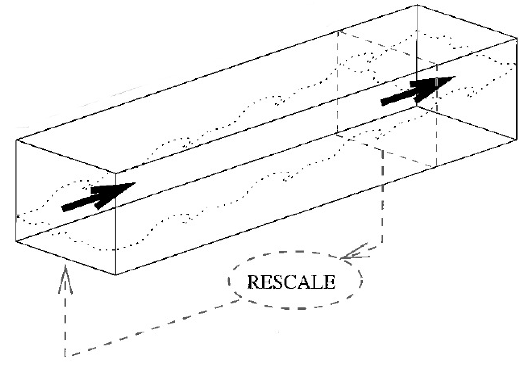
In this section, we evaluate the effect of the three recycling-rescaling methods, the effect of wall temperature, and the effect of number of cells in the boundary layer. In

Table 2. Grid Properties for the Slightly Cold Wall Flat Plate.

Grid	$\Delta \mathit{x}$	$\Delta {\mathit{y}}_{\mathit{min}}$	$\Delta \mathit{z}$	$\Delta {\mathit{x}}^{+}$	$\Delta {\mathit{y}}^{+}$	$\Delta {\mathit{z}}^{+}$	${\mathit{L}}_{\mathit{x}}/\mathit{\delta }$	${\mathit{L}}_{\mathit{y}}/\mathit{\delta }$	${\mathit{L}}_{\mathit{z}}/\mathit{\delta }$	Cells
	$\left(\mathsf{\mu }\mathbf{m}\right)$	$\left(\mathsf{\mu }\mathbf{m}\right)$	$\left(\mathsf{\mu }\mathbf{m}\right)$
1	96.5	4.82	96.5	10	0.5	10	29.5	4.00	4.22	6.6 M
2	74.8	3.74	74.8	10	0.5	10	22.8	2.85	3.27	5.8 M
2(b)	74.8	3.74	74.8	10	0.5	10	22.8	2.95	3.27	8.7 M
3	45.15	2.26	45.15	10	0.5	10	22.8	3.16	3.26	16.9 M

, the grid properties of the four grids used in this paper are present, where $L_x$, $L_y$, and $L_z$ are respectively the dimensions of the computational region in the streamwise, wall normal, and spanwise directions. Grid 1 is used for freestream Condition 1, Grids 2 and 2(b) are used for Condition 2, and Grid 3 is used for Condition 3.

3.1. Effect of the Recycling-Rescaling Method

In this section the effect of the three different recycling-rescaling methods on the prediction of turbulent properties is examined. To do so, the freestream properties are the same as Condition 2 of Table 1 and the grid is Grid 2. The calculated velocity profile, Reynolds Analogy Factor, Strong Reynolds Analogy, turbulent Prandtl number, dimensionless turbulent shear stress, turbulent normal stresses in streamwise, wall normal, and spanwise directions, and energy spectra are examined to evaluate the different recycling-rescaling models and the performance of the proposed method of $H_t\&p$.

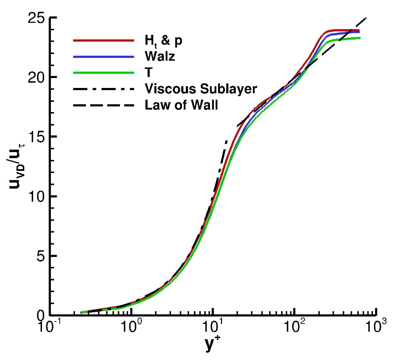
Figure 2 shows the calculated mean streamwise velocity and the Van Driest transformed Law of the Wall at $x/\delta =20$. The continuous lines are calculated mean streamwise velocity of the the three recycling-rescaling methods, namely $H_t\&p$, Walz, and T. The dashed-dotted line is is the Van Driest transformed velocity in the viscous sublayer, and the dashed line is the Van Driest transformed velocity of the Law of the Wall. The calculated mean streamwise velocity of all three recycling-rescaling methods agree well with the Van Driest transformed velocity of viscous sublayer and Law of the Wall.

Table 3. Effect of recycling-rescaling method on Reynolds Analogy Factor ($2St/C_f$) for condition No. 2.

	${\mathit{H}}_{\mathit{t}}\&\mathit{p}$	Walz	T	Conventional
$2St/C_f$	1.21	1.33	0.95	1.12

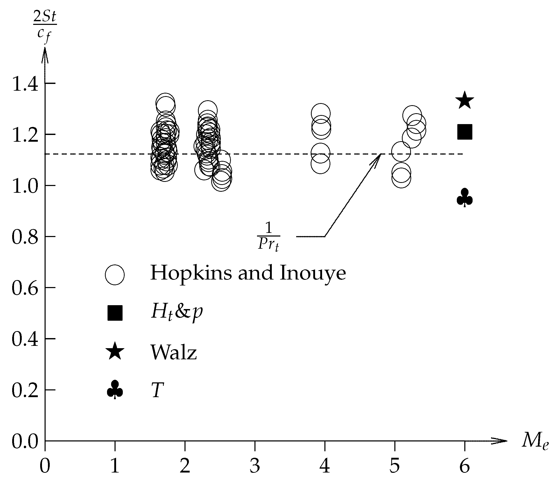
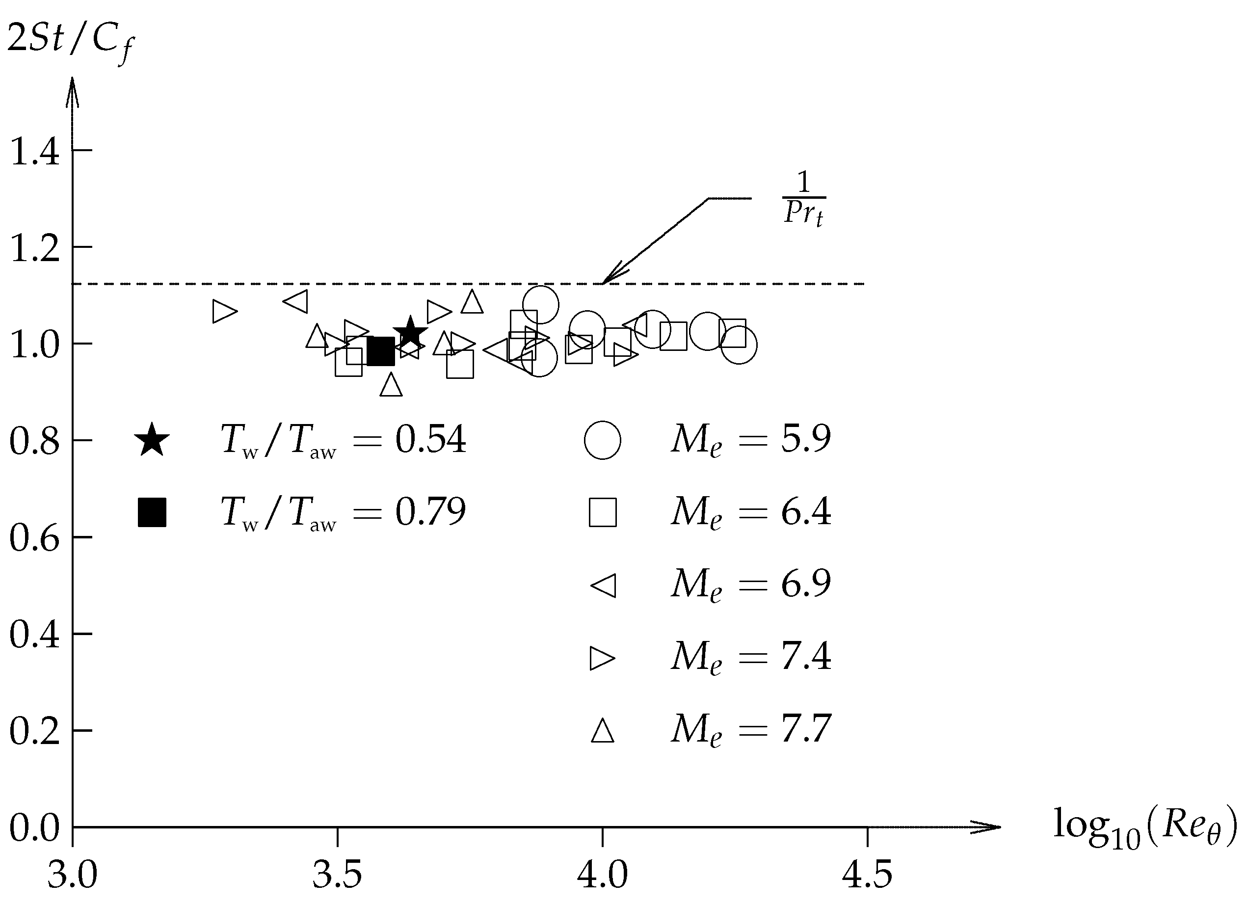
presents the Reynolds Analogy Factor of each recycling-rescaling method. The conventional value ($2St/C_f=P{r}_t^{-1}=1.12$ with $P{r}_t=0.89$) is also provided. Figure 3 shows the experimental scattering of Reynolds Analogy Factor versus Mach number [39]. The calculated Reynolds Analogy Factors by the three methods are within the experimental uncertainty of experimental data.

To examine the effect of the recycling-rescaling method on the calculated Strong Reynolds Analogy, the Strong Reynolds Analogies proposed by Morkovin [40] and Huang [41] are selected. The Morkovin Strong Reynolds Analogy [40] is

$$\frac{\sqrt{\overline{T^{\prime 2}}}/\overline{T}}{(\gamma -1){\overline{M}}^2\sqrt{\overline{u^{\prime 2}}}/\overline{u}}=1.$$

(41)

The Huang Strong Reynolds Analogy [41] is

$$\frac{\sqrt{\overline{T^{\prime 2}}}/\overline{T}}{(\gamma -1){\overline{M}}^2\sqrt{\overline{u^{\prime 2}}}/\overline{u}}=\frac{1}{P{r}_t}\frac{1}{\left|d\overline{T_t}/d\overline{T}-1\right|},$$

(42)

where,

$$\overline{T_t}\approx \overline{T}+\frac{{\overline{u}}^2}{2c_p},$$

(43)

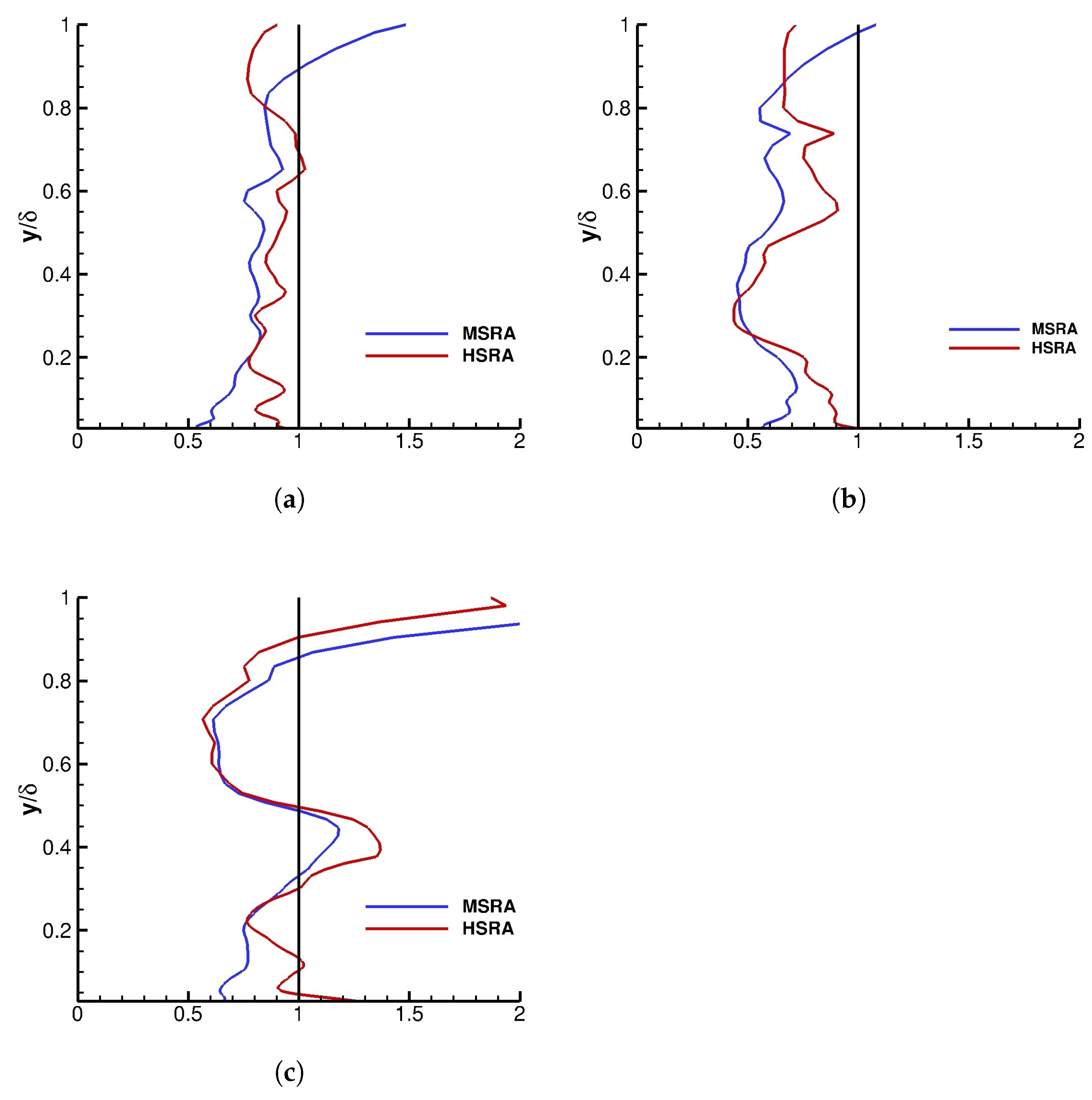
and $P{r}_t=0.89$. Figure 4 presents the two Strong Reynolds Analogies evaluated at $x/\delta =20$. In each graph, the blue lines are the $\mathrm{MSRA}$, where $\mathrm{MSRA}$ is calculated by

$$\mathrm{MSRA}=\frac{\sqrt{\overline{T^{\prime 2}}}/\overline{T}}{(\gamma -1){\overline{M}}^2\sqrt{\overline{u^{\prime 2}}}/\overline{u}}.$$

(44)

The red lines are the $\mathrm{HSRA}$, where $\mathrm{HSRA}$ is calculated by

$$\mathrm{HSRA}=\left(\frac{\sqrt{\overline{T^{\prime 2}}}/\overline{T}}{(\gamma -1){\overline{M}}^2\sqrt{\overline{u^{\prime 2}}}/\overline{u}}\right)/\left(\frac{1}{P{r}_t}\frac{1}{\left|d\overline{T_t}/d\overline{T}-1\right|}\right).$$

(45)

The black line is the line of constant value one. The closer the $\mathrm{MSRA}$ and $\mathrm{HSRA}$ are to the line of constant one (i.e., the black line), the better is the prediction. In general, Huang Strong Reynolds Analogy is a better estimate than Morkovin Strong Reynolds Analogy which is in agreement with the DNS results of Duan et al. [42]. Importantly, the best agreement of the Morkovin and Huang Reynolds Analogy is for the $H_t\&p$ recycling-rescaling method.

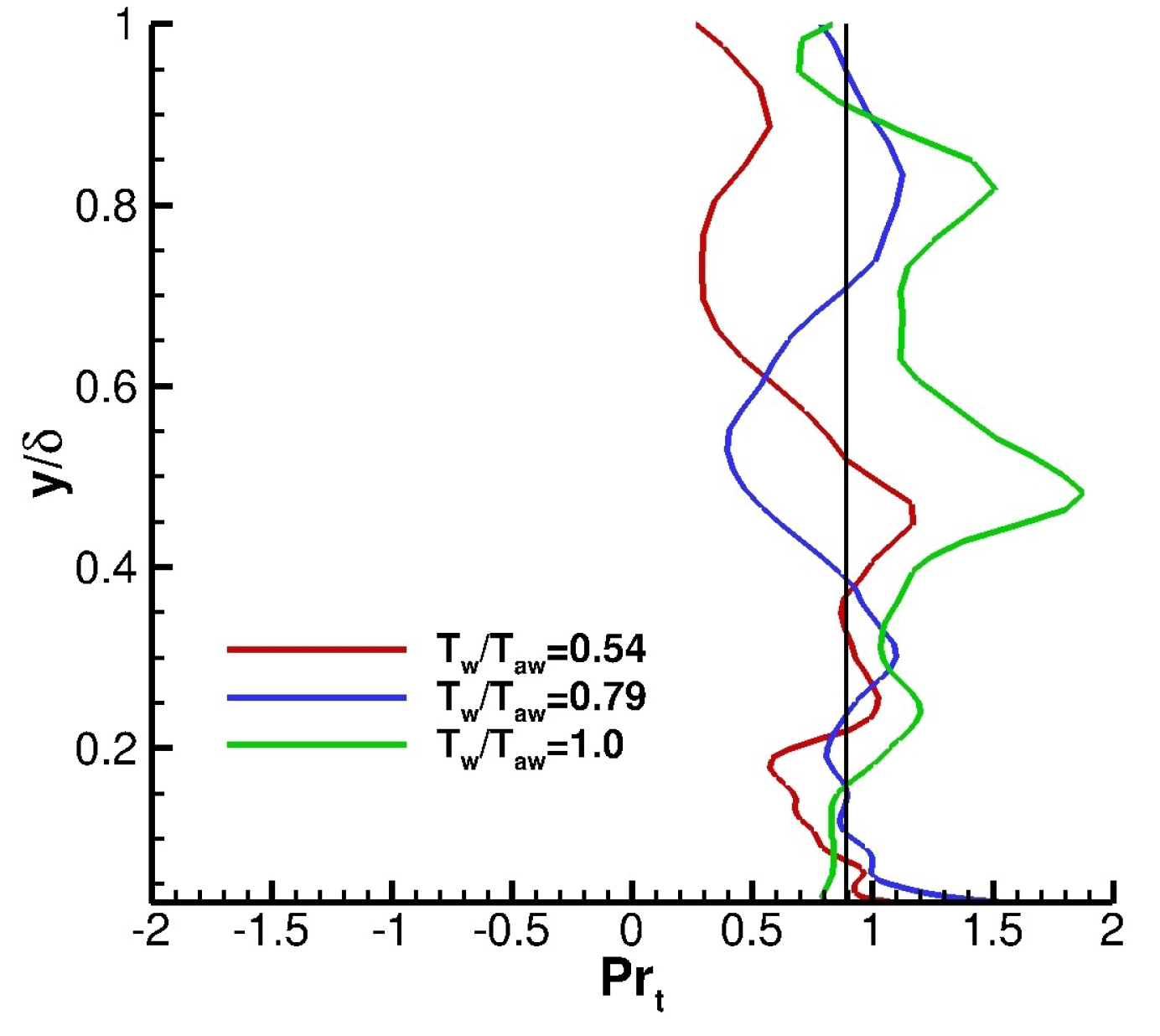
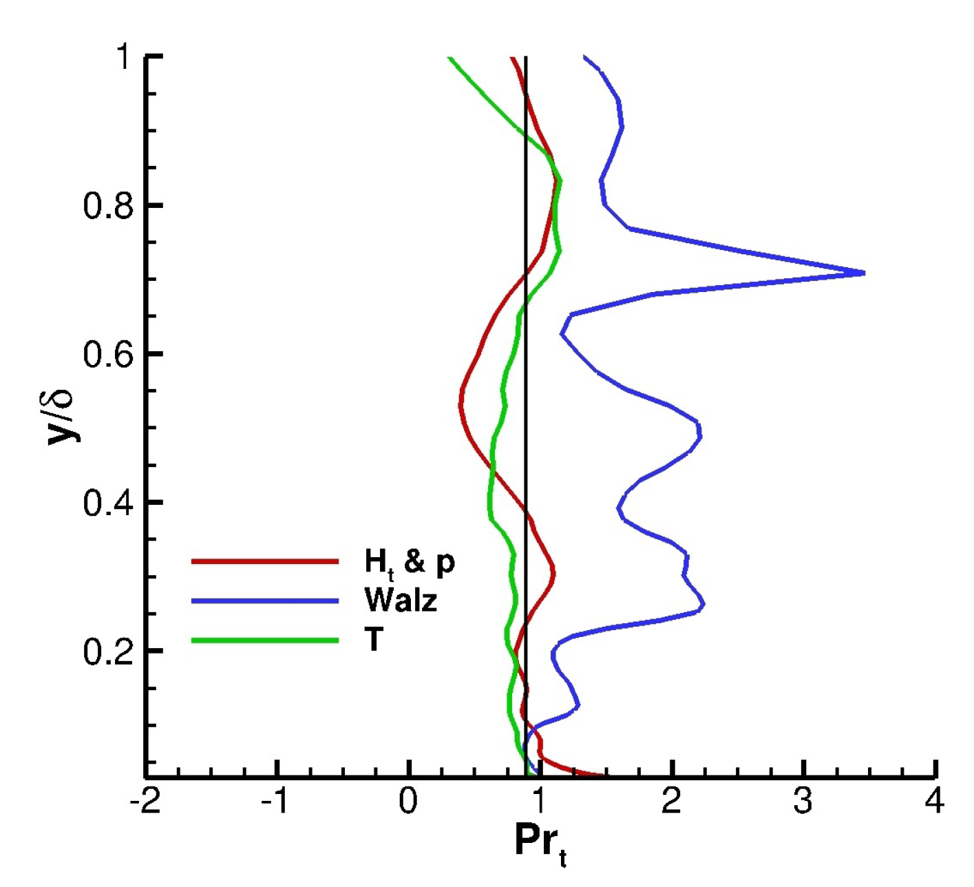
Figure 5 shows the calculated turbulent Prandtl number by the three recycling-rescaling methods evaluated at $x/\delta =20$. The Prandtl number in a turbulent boundary layer is defined as

$$P{r}_t=\frac{\overline{\rho u^{\prime }{v}^{\prime }}\partial \overline{T}/\partial y}{\overline{\rho v^{\prime }{T}^{\prime }}\partial \overline{u}/\partial y}.$$

(46)

The black line in the figure is the constant Prandtl number of 0.89. The calculated turbulent Prandtl number of $H_t\&p$ and T methods are closer to this line in comparison to the Walz method. According to DNS results of Zhang et al. [43], although the turbulent Prandtl number is not constant in the boundary layer, it stays close to the conventional value of 0.89.

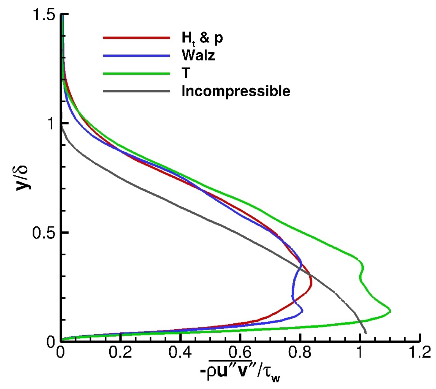
Figure 6 presents the calculated Morkovin scaled dimensionless turbulent shear stress ($-\overline{\rho u^{″}{v}^{″}}/{\tau }_{\mathrm{w}}$) by the three recycling-rescaling methods at $x/\delta =20$. Additionally, for comparison purposes, the incompressible shear stress data of Klebanoff [44] is also presented. The predicted Morkovin scaled dimensionless turbulent shear stresses are in general agreement with the incompressible data although the region with non-zero turbulent shear stress is smaller in the incompressible data. The Morkovin scaled dimensionless turbulent shear stress is zero at the wall, increases to its maximum value of about one at some distance near the wall and then reduces to zero at the edge of the boundary layer. The Walz and $H_t\&p$ methods predict the same maximum turbulent shear stress while the T method predicts a larger maximum shear stress.

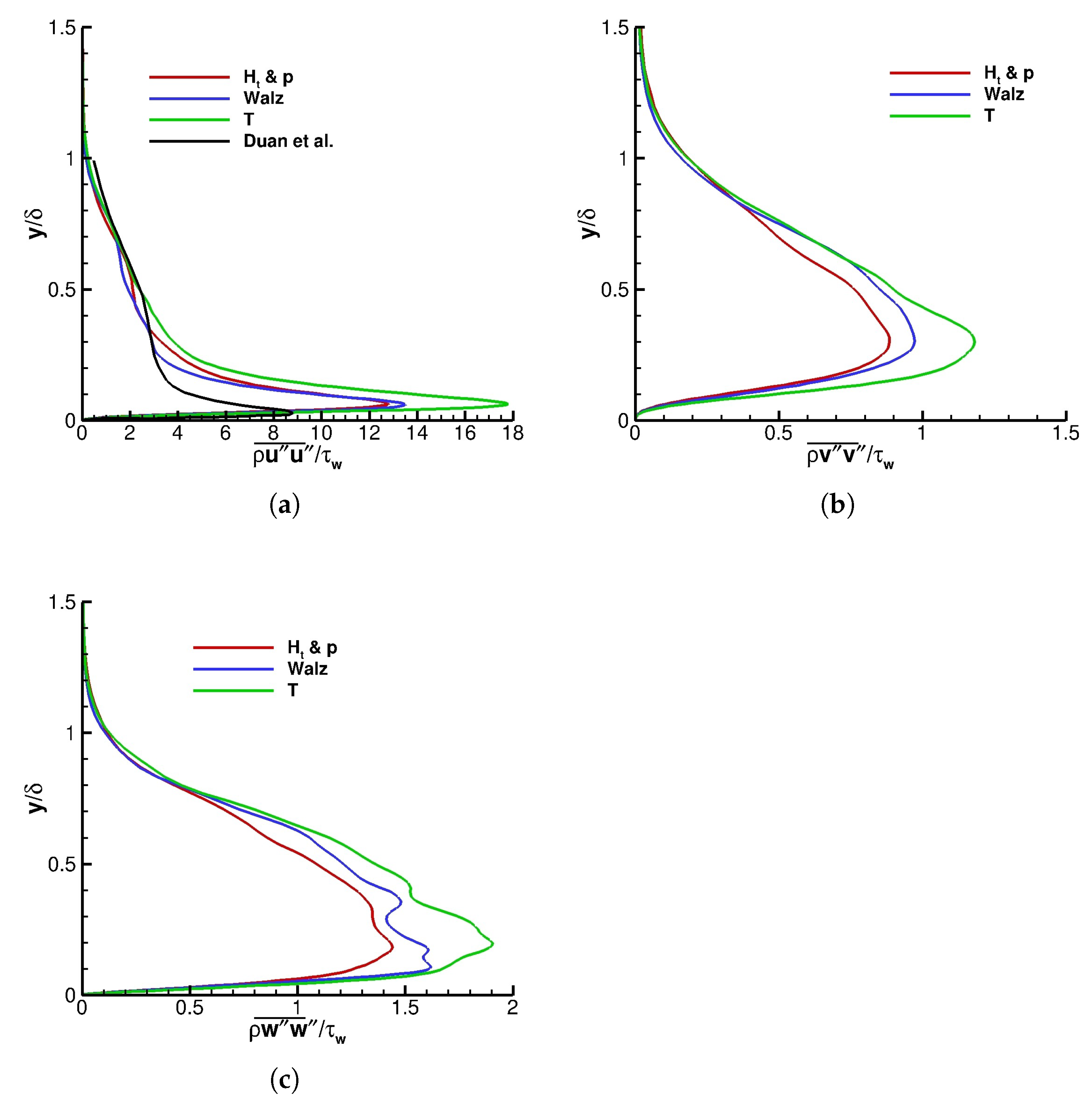
Figure 7 shows the predicted Morkovin scaled dimensionless turbulent normal stresses ($\overline{\rho u_i^{″}{u}_i^{}}/{\tau }_{\mathrm{w}}$, $i=1,2,3$) respectively in streamwise, wall normal, and spanwise directions by the three recycling-rescaling methods at $x/\delta =20$. All the methods predict the same behavior for the turbulent normal stresses. In the outer part of boundary layer, the Morkovin scaled dimensionless turbulent normal stresses are essentially the same for all three methods. However, the T method predicts the largest peak normal stresses for each of the Morkovin scaled dimensionless turbulent normal stresses while $H_t\&p$ method has the smallest peaks.

The comparison of the predicted Morkovin scaled dimensionless turbulent streamwise stress with the DNS results of Duan et al. [42] shows a general agreement; however, the maximum stress is smaller for Duan et al. Further investigation is required to understand the reason behind this. It should be mentioned here that $T_{\mathrm{w}}/T_{\mathrm{a}\mathrm{w}}$ for the presented result of Duan et al. is 0.68 while in our case, $T_{\mathrm{w}}/T_{\mathrm{a}\mathrm{w}}$ is 0.79.

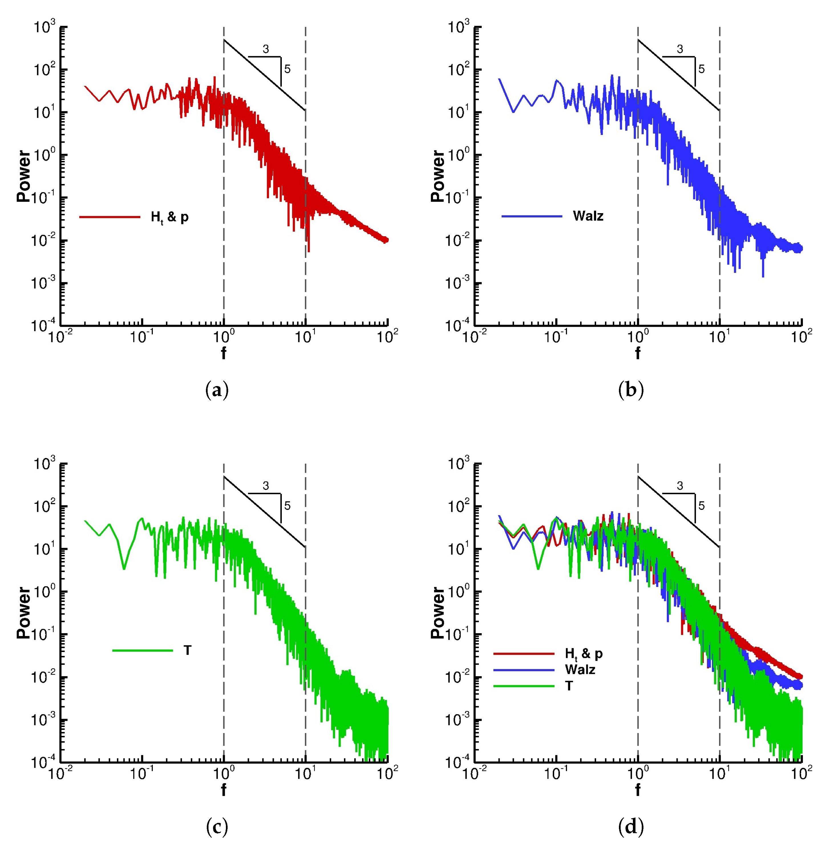
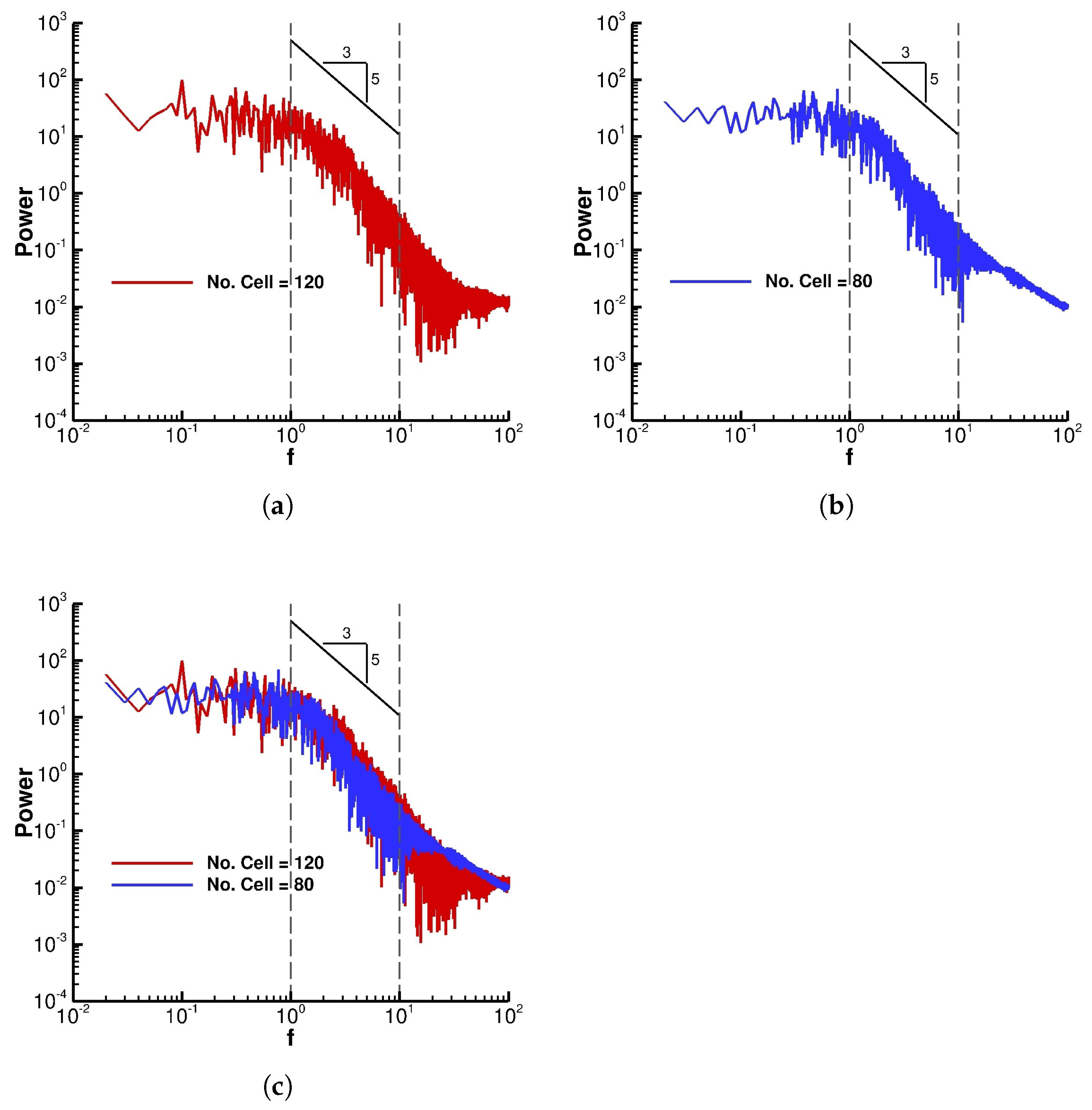
Figure 8 presents the energy spectrum of the total energy per unit mass of the three recycling-rescaling methods at $x/\delta =20$ and $y/\delta =0.7$ for the dimensionless time interval $\Delta t{U}_{\infty }/\delta =100$. The inertial subrange for this problem is between dimensionless frequencies ($f=f^{\ast }\delta /U_{\infty }$) of 1 and 10. From these graphs, all three methods predict the slope of the energy spectrum of $-5/3$ in the inertial subrange. The slope $-5/3$ is the theoretical prediction for the energy spectrum slope at the inertial subrange.

In summary, the introduced $H_t\&p$ recycling-rescaling method has a better prediction of the turbulent properties. The $H_t\&p$ method has the best prediction for Strong Reynolds Analogy and turbulent Prandtl number compared to the Walz and T methods and has comparable results for Law of the Wall, Reynolds Analogy Factor, turbulent shear and normal stresses, and energy spectrum. Therefore, the $H_t\&p$ method is used for the recycling-rescaling in the rest of the paper.

3.2. Effect of Wall Temperature

In this section, the proposed $H_t\&p$ recycling-rescaling method is used to calculate the turbulent properties at different wall temperatures. Conditions 1 to 3 of Table 1 are considered. The Grids 1, 2, and 3 of Table 2 are used respectively for Conditions 1, 2, and 3. Table 2 shows that the LES calculation becomes computationally expensive as the wall temperature decreases. Decreasing the wall temperature from adiabatic wall ($T_{\mathrm{a}\mathrm{w}}$) to 0.54$T_{\mathrm{a}\mathrm{w}}$, the grid spacing normal to the wall decreases by a factor of 2.13 to keep the same $\Delta y^{+}$.

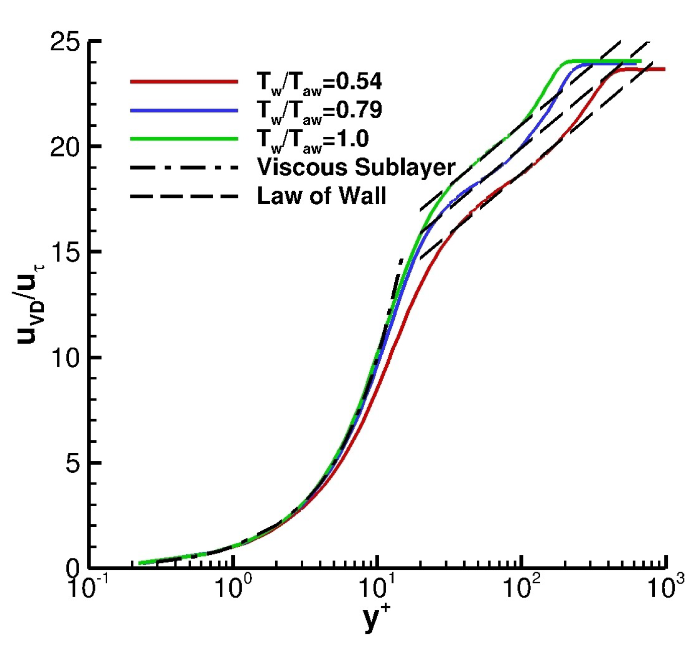
Figure 9 shows the calculated Law of the Wall at $x/\delta =20$ for the three wall temperatures. The continuous lines are the Van Driest transformed mean streamwise velocity at $T_{\mathrm{w}}/T_{\mathrm{a}\mathrm{w}}$ of 0.54, 0.79, and 1.0. Additionally, the dashed lines show the Law of the Wall for each wall temperature and the dashed-dotted line is the Van Driest transformed velocity at viscous sublayer. The predicted Van Driest transformed velocity agrees well with the Van Driest transformed velocities of the viscous sublayer and Law of the Wall for all three wall temperature. Increasing the wall temperature increases the constant C in the logarithmic region. 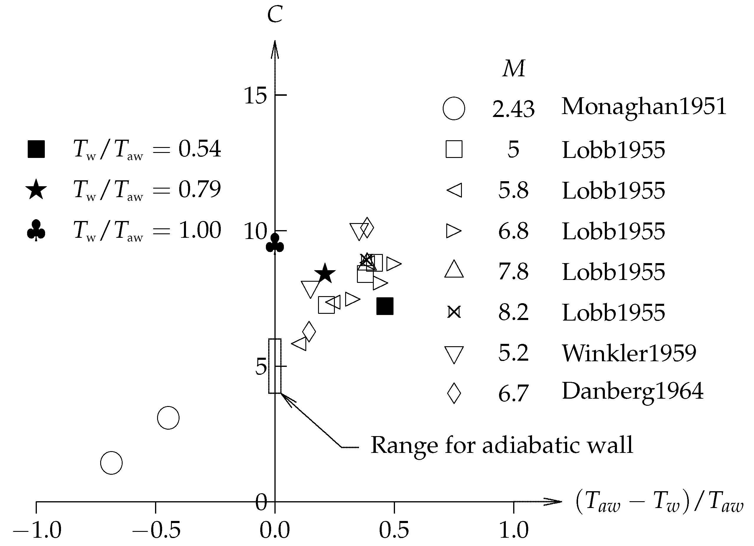The constant C in the Law of the Wall is 7.2, 8.4, and 9.5 respectively for $T_{\mathrm{w}}/T_{\mathrm{a}\mathrm{w}}$ of 0.54, 0.79, and 1.0. This trend is in opposition with the trend reported by Danberg [32] as shown in Figure 10.

Table 4. Effect of wall temperature on boundary layer displacement and momentum thickness.

	${\mathit{T}}_{\mathbf{w}}/{\mathit{T}}_{\mathbf{aw}}=0.54$	${\mathit{T}}_{\mathbf{w}}/{\mathit{T}}_{\mathbf{aw}}=0.79$	${\mathit{T}}_{\mathbf{w}}/{\mathit{T}}_{\mathbf{aw}}=1.00$
${\delta }^{\ast }/\delta$	10.4312 ± 0.00004	10.4658 ± 0.00027	10.5344 ± 0.0018
$\theta /\delta$	10.0428 ± 0.00028	10.0357 ± 0.00027	10.0322 ± 0.00046
H	10.07 ± 0.07	13.1 ± 0.1	16.8 ± 0.6

presents the values of the compressible turbulent boundary layer displacement (${\delta }^{\ast }$) and momentum ($\theta$) thicknesses, as well as the shape factor $H={\delta }^{\ast }/\theta$ for all three wall temperature. Decreasing the wall temperature decreases the displacement thickness while increasing the momentum thickness and decreasing the shape factor.

Table 5. Effect of wall temperature on Reynolds Analogy Factor ($2St/C_f$).

	${\mathit{T}}_{\mathit{w}}/{\mathit{T}}_{\mathbf{aw}}=0.54$	${\mathit{T}}_{\mathit{w}}/{\mathit{T}}_{\mathbf{aw}}=0.79$	Conventional
$2St/C_f$	1.02	0.98	1.12

presents the Reynolds Analogy Factor for $T_{\mathrm{w}}/T_{\mathrm{a}\mathrm{w}}$ of 0.54 and 0.79. Again, the conventional value ($2St/C_f=P{r}_t^{-1}=1.12$) for Reynolds Analogy Factor is also presented in the table. The predictions are within the experimental uncertainty of available experimental data in the literature. Figure 11 shows a sample of the Reynolds Analogy Factor from the literature where the open symbols are from Keener and Polek [45].

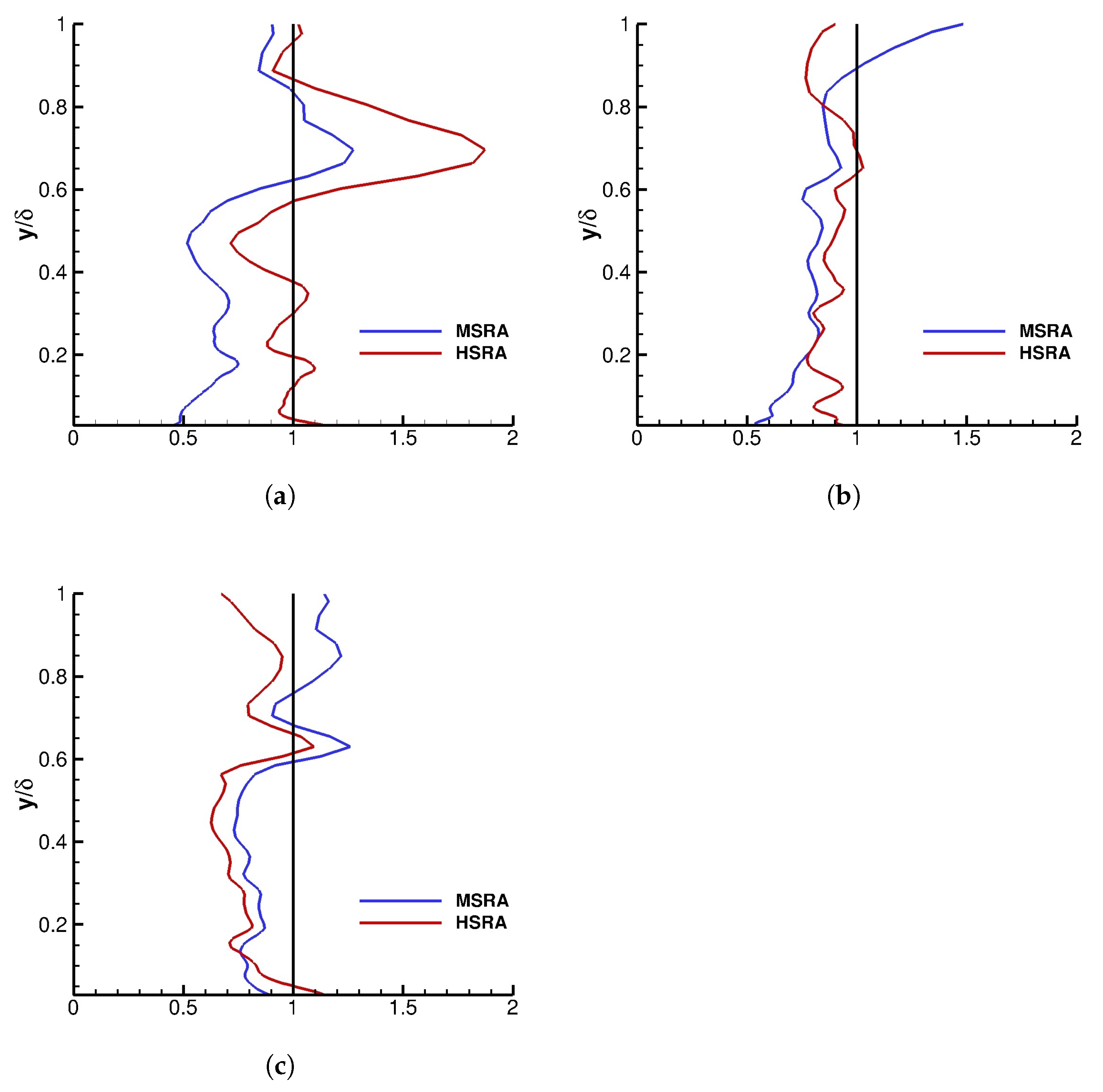
Figure 12 shows the Morkovin and Huang Strong Reynolds Analogies for the three wall temperature $T_{\mathrm{w}}/T_{\mathrm{a}\mathrm{w}}$ of 0.54, 0.79, and 1.0 evaluated at $x/\delta =20$. In each graph, the blue lines are the $\mathrm{MSRA}$ calculated by Equation (44), the red lines are the $\mathrm{HSRA}$ calculated by Equation (45), and the black lines are the constant value of one. The turbulent Prandtl number ($P{r}_t$) is 0.89. In general, the Huang Strong Reynolds Analogy is a better estimate compared to the Morkovin Strong Reynolds Analogy. Moreover, the Huang Strong Reynolds Analogy is more accurate for the cold wall condition. In other words, the accuracy of Huang Reynolds Analogy is reduced by increasing the wall temperature, especially in the inner region.

Figure 13 shows the calculated turbulent Prandtl number (Equation (46)) for the three wall temperatures. The black line represents the constant turbulent Prandtl number of 0.89. The calculated turbulent Prandtl number remains close to the constant line of 0.89, especially in the inner region.

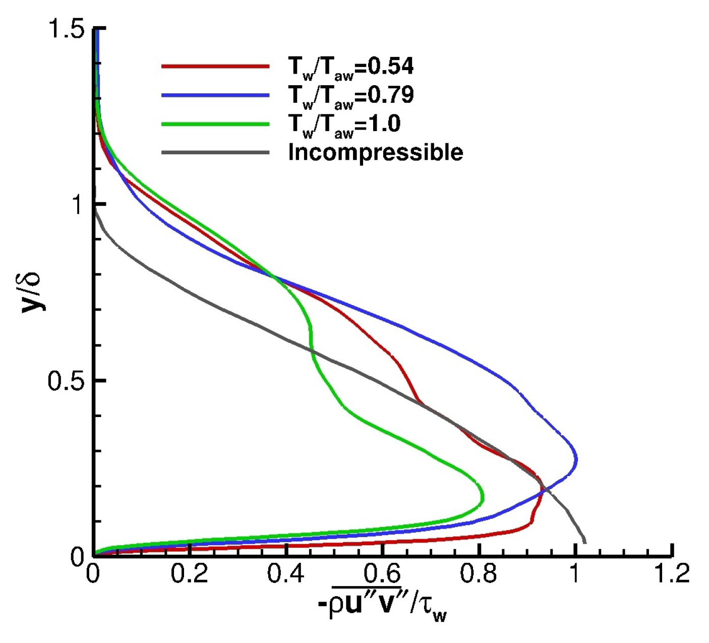
Figure 14 presents the Morkovin scaled dimensionless turbulent shear stress ($-\overline{\rho u^{″}{v}^{″}}/{\tau }_{\mathrm{w}}$) at $x/\delta =20$ for three wall temperature $T_{\mathrm{w}}/T_{\mathrm{a}\mathrm{w}}$ of 0.54, 0.79, and 1.0. The black line in the figure is the incompressible turbulent shear stress from Klebanoff [44]. For all wall temperatures, the Morkovin scaled dimensionless turbulent shear stress is zero at the wall and increases by increasing distance from the wall until it reaches its maximum value and then starts decreasing until reaching to zero at the edge of the boundary layer. The results have the same behavior as the incompressible data; however, the region with non-zero turbulent stress is larger in the compressible results.

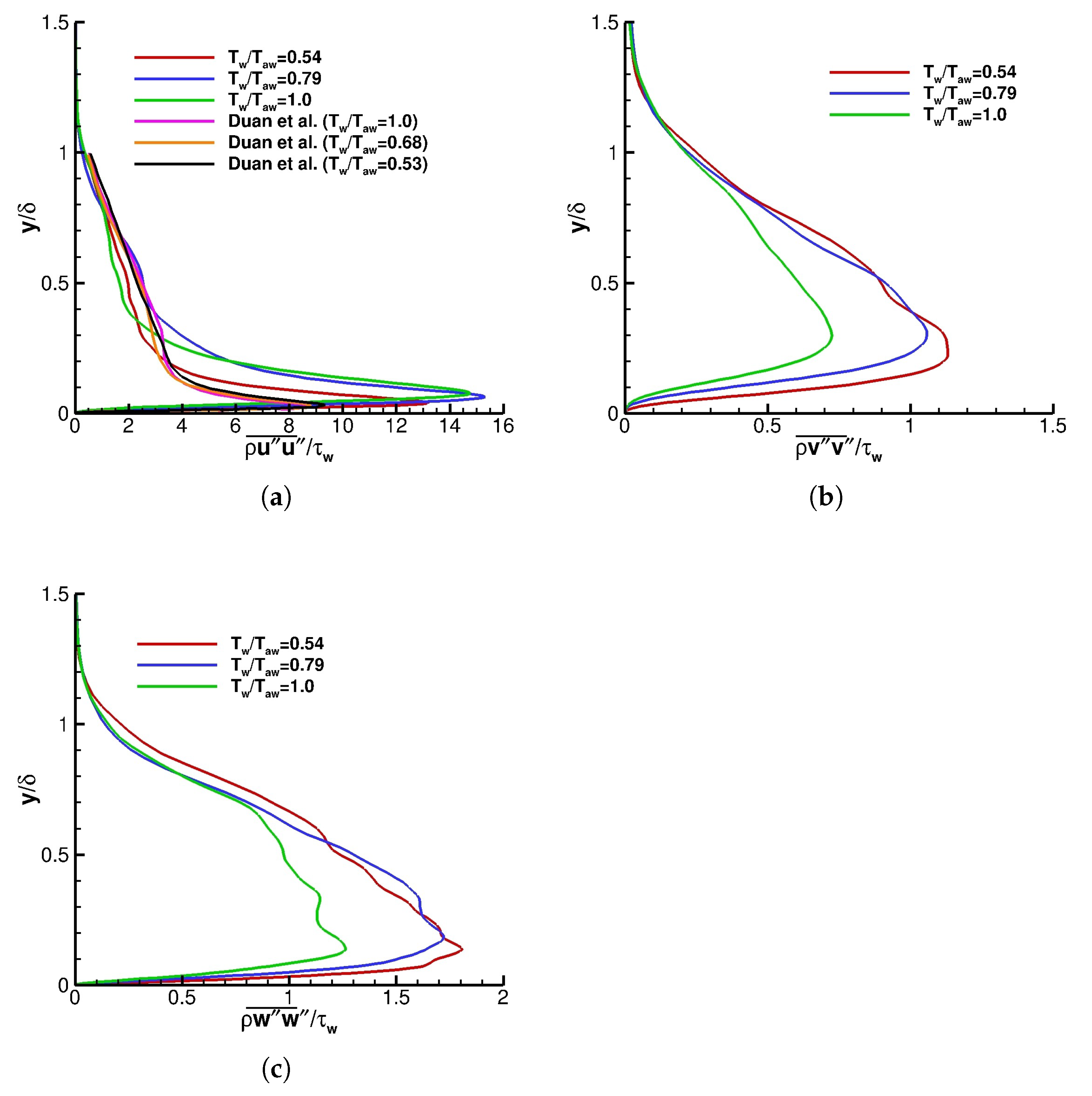
Figure 15 shows the Morkovin scaled dimensionless turbulent normal stresses ($\overline{\rho u_i^{″}{u}_i^{″}}/{\tau }_{\mathrm{w}}$) in streamwise, wall normal, and spanwise directions. Additionally, the DNS results of Duan et al. [42] for the Morkovin scaled dimensionless turbulent streamwise stress for three wall temperatures are also presented. From the figure, in the outer region, the Morkovin scaled dimensionless turbulent normal stresses are independent of wall temperature. However, in the inner region, where the peak normal stresses are located, increasing the wall temperature decreases the maximum wall normal and spanwise turbulent stresses while increasing the streamwise turbulent stress.

Additionally, increasing the wall temperature moves the location of maximum turbulent streamwise stress away from the wall. It should be mentioned here that the Morkovin scaled dimensionless turbulent streamwise stress yields almost the same peak value and peak location for the $T_{\mathrm{w}}/T_{\mathrm{a}\mathrm{w}}$ of 0.79 and 1.0. However, the DNS results of Duan et al. shows no significant dependence to the wall temperature.

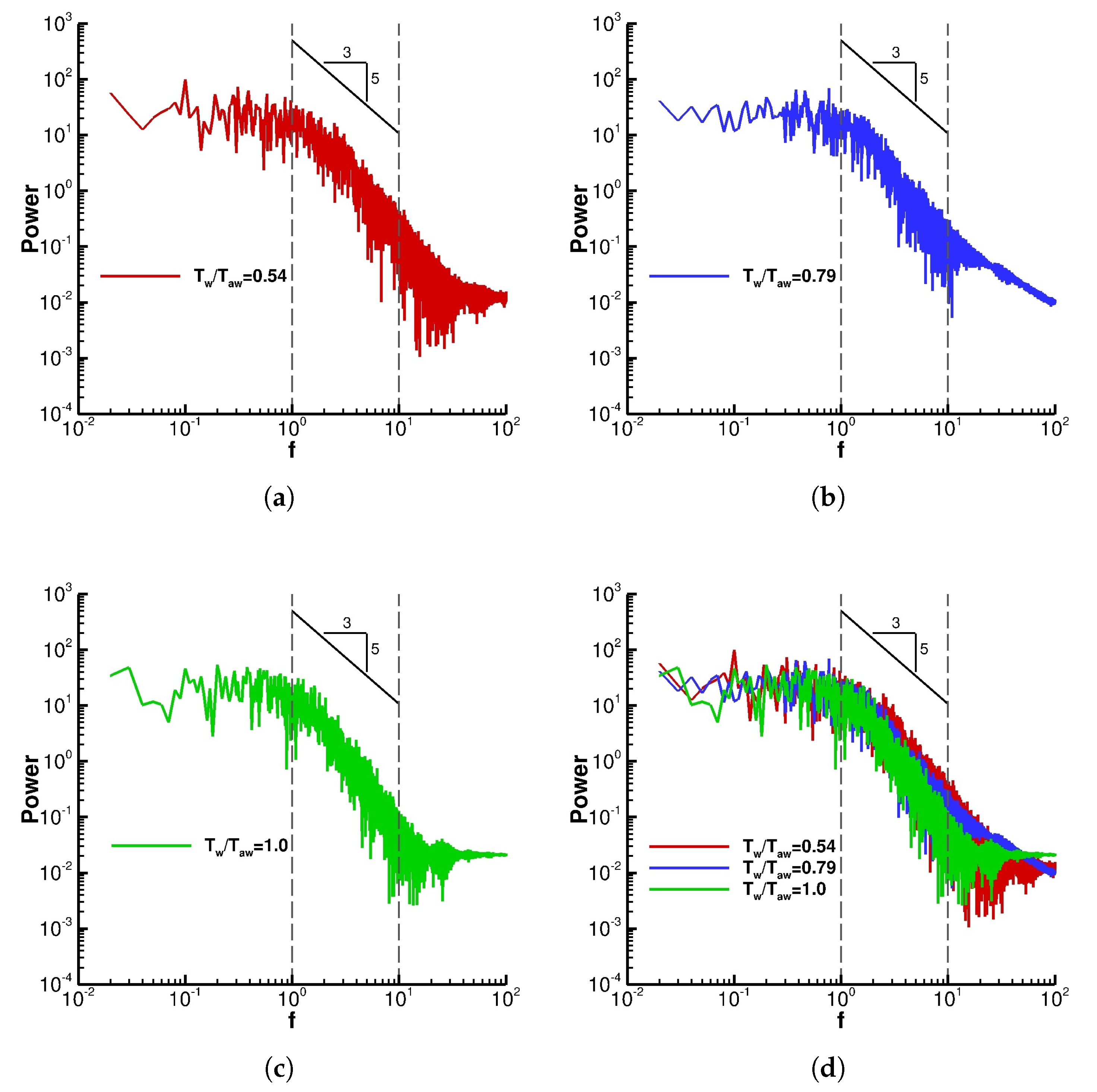
Figure 16 represents the energy spectrum of the total energy per unit mass at $x/\delta =20$ and $y/\delta =0.7$ over the dimensionless time interval of 100 for three wall temperatures. The range of dimensionless frequencies for the inertial subrange is 1 to 10. It can be seen that the slope of the energy spectrum in the inertial subrange for all the wall temperatures is $-5/3$. This slope of $-5/3$ is what is expected for the inertial subrange in the theory.

3.3. Effect of The Number of Cells in the Boundary Layer

In this section, the effect of the grid is examined by changing the number of cells in the wall normal direction in the boundary layer. For this purpose, two grids, namely Grids 2 and 2(b) of Table 2 are used for Condition 2 of Table 1. The grids have the same $y^{+}$ near the wall and then are stretched using geometric stretching until reaching the edge of the boundary layer. Grid 2 and 2(b) respectively have 80 and 120 cells in the wall normal direction in the boundary layer. The different number of cells in the wall normal direction means that the stretching factor is smaller in Grid 2(b) and thus, the grid cells are smaller in size in the boundary layer in comparison to Grid 2. Both calculations are performed using $H_t\&p$ recycling-rescaling method.

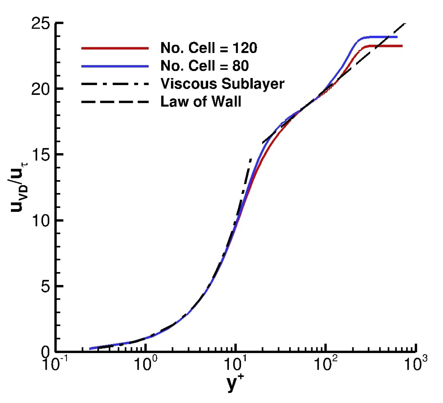
Figure 17 shows the comparison of the calculated Van Driest transformed mean streamwise velocity with the Law of the Wall at $x/\delta =20$. Additionally, the dashed line in the figure represents the Law of Wall, and the dashed dotted line represents the viscous sublayer. The calculated Van Driest transformed streamwise velocity of both grids are in good agreement with the theoretical values for Law of Wall and viscous sublayer. It is worth mentioning here that the $u_{\tau }$ for both grids is essentially the same and the difference is less than a percent.

Table 6. Effect of Number of Cells in the Boundary Layer on Reynolds Analogy Factor ($2St/C_f$) for Condition No. 2.

	$\mathit{j}=120$	$\mathit{j}=80$	Conventional
$2St/C_f$	0.98	1.02	1.12

shows the Reynolds Analogy Factor for the two grids with 80 and 120 cells in the wall normal direction in the boundary layer. Additionally, the conventional value of Reynolds Analogy Factor ($2St/C_f=P{r}_t^{-1}=1.12$) is also presented. Both grids have the Reynolds Analogy Factor within the range of the experimental uncertainty in the literature (see Figure 11).

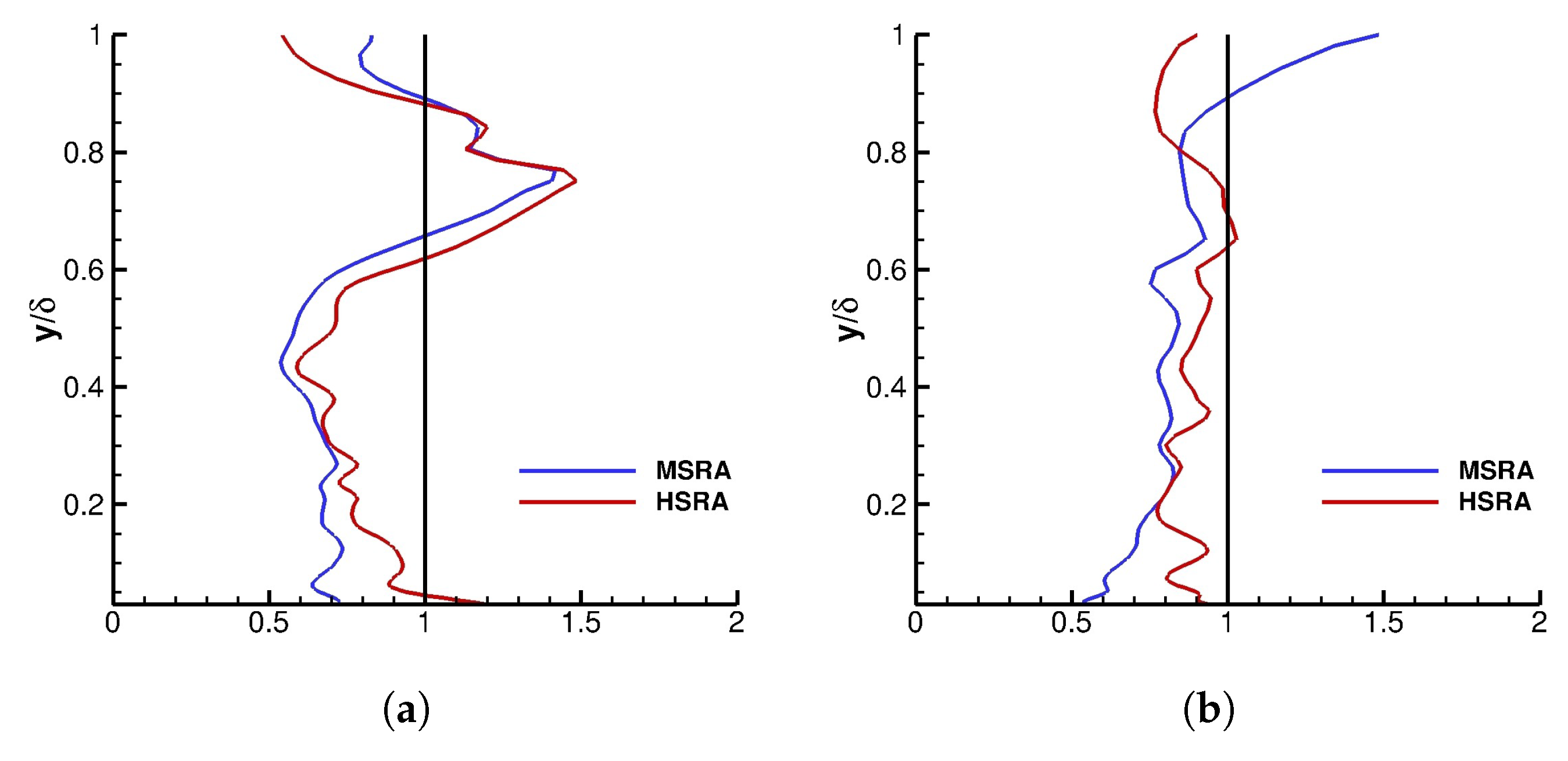
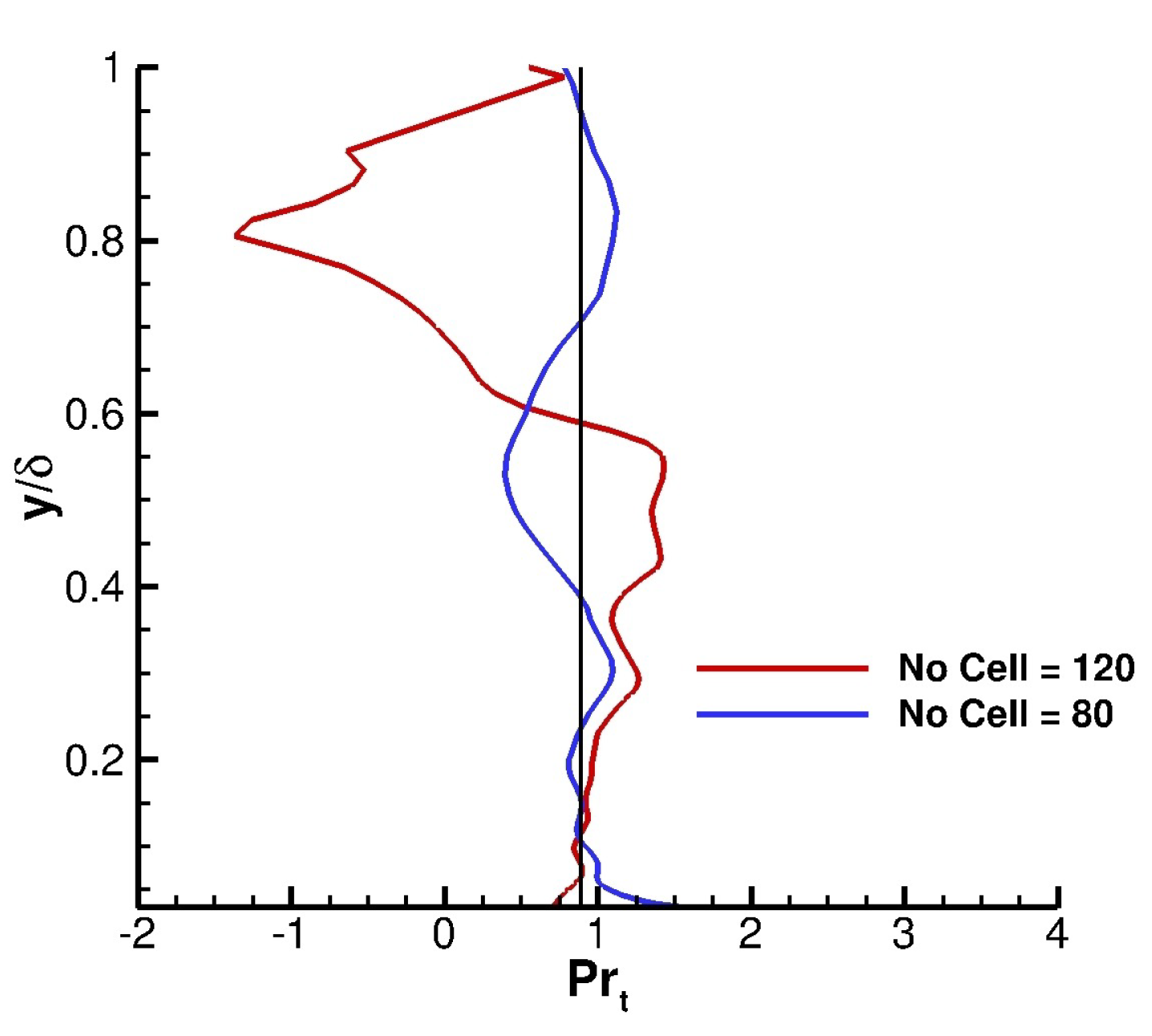
Figure 18 shows the Morkovin and Huang Strong Reynolds Analogies for the two grids with 80 and 120 cells in the wall normal direction inside the boundary layer. In each graph, the blue line is the $\mathrm{MSRA}$ calculated by Equation (44), the red line is the $\mathrm{HSRA}$ calculated by Equation (45), and the black line is the line of constant value one. The turbulent Prandtl number in the Strong Reynolds Analogy is $P{r}_t=0.89$. The Huang Strong Reynolds Analogy has a better result as expected. Surprisingly, the grid with 80 cells in the wall normal direction inside the boundary layer has better prediction of the Strong Reynolds Analogy compared to having a finer grid with 120 cells in the wall normal direction inside the boundary layer.

Figure 19 presents the calculated turbulent Prandtl number for the two grids with 80 and 120 cells in the wall normal direction inside the boundary layer. Additionally, the constant turbulent Prandtl number of 0.89 is also presented by a black line. In general, both grids have the Prandtl number close to the constant turbulent Prandtl number of 0.89. In the inner region, both grids have good agreement with each other; however, in the outer region the grid with 80 cells in wall normal direction inside the boundary layer stays closer to the constant line of 0.89.

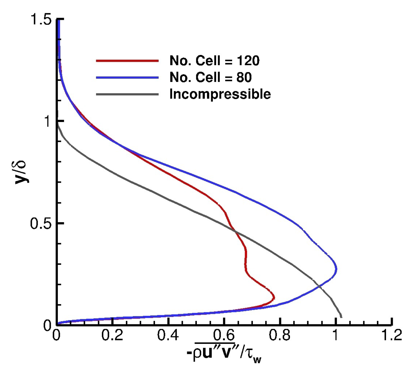
Figure 20 presents the Morkovin scaled dimensionless turbulent shear stress ($-\overline{\rho u^{″}{v}^{″}}/{\tau }_{\mathrm{w}}$) for the two grids with 80 and 120 cells in the wall normal direction inside the boundary layer. For comparison purposes, the incompressible dimensionless shear stress values of Klebanoff [44] are also presented. Once again, the compressible data have a larger region with non-zero shear stresses. However, the compressible and incompressible data have the same trends. Moreover, the maximum shear stress is larger for the grid with 80 cells compared to the grid with 120 cells in the wall normal direction inside the boundary layer. It is worth mentioning here that the $u_{\tau }$ for both grids is essentially the same.

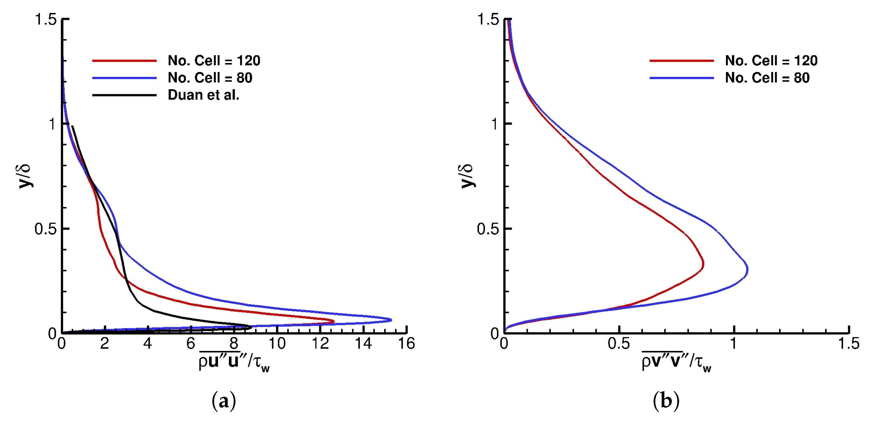
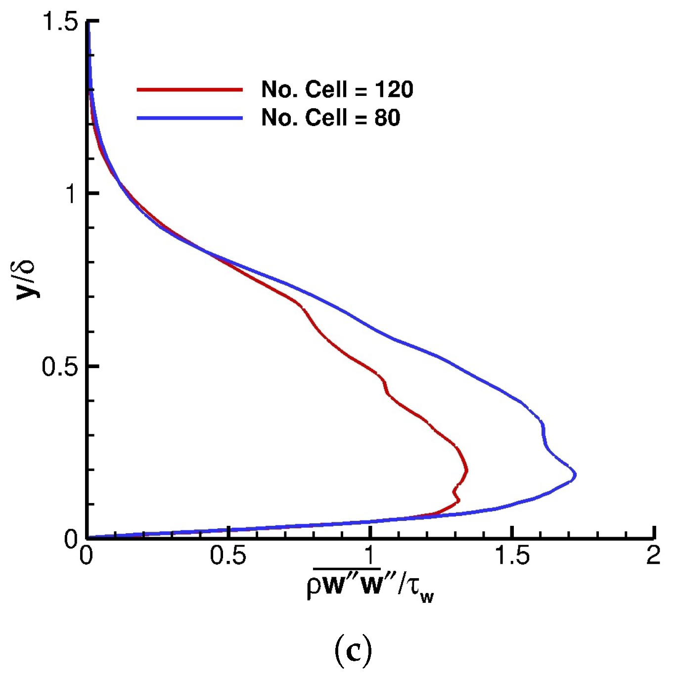
Figure 21 shows the Morkovin scaled dimensionless turbulent normal stresses ($\overline{\rho u_i^{″}{u}_i^{″}}/{\tau }_{\mathrm{w}}$) in streamwise, wall normal, and spanwise directions for two grids with 80 and 120 cells in the wall normal direction inside the boundary layer. It can be seen that the thickness of the layer normal to the wall with non-zero normal stresses are the same for both grids. Moreover, the maximum values of the turbulent normal stresses decreases by increasing the number of cells in the wall normal direction. Comparison of the results with the DNS results of Duan et al. [42] shows similar trend; however, the peak value of the wall normal stress is smaller in Duan et al. calculations.

Figure 22 presents the energy spectrum of the total energy per unit mass for two grids with 80 and 120 cells in the wall normal direction inside the boundary layer at $x/\delta =20$ and $y/\delta =0.7$ over the dimensionless time interval of 100. The inertial subrange for this problem is bounded by dimensionless frequencies ($f=f^{\ast }\delta /U_{\infty }$) of 1 and 10. From the figure it can be seen that both grid predict the slope of $-5/3$ in the inertial subrange. This slope of $-5/3$ is the theoretical value for the slope of the inertial subrange.

4. Conclusions

A new recycling-rescaling method is evaluated for generation of the instantaneous time-dependent inflow boundary. The new method considers the change in the pressure along the boundary layer and recycles total enthalpy, static pressure, and three components of velocity. This method is compared with two more traditional ways of recycling-rescaling by comparing the Law of the Wall, Reynolds Analogy Factor, Morkovin and Huang Strong Reynolds Analogy, turbulent Prandtl number, turbulent shear stress, turbulent normal stresses, and energy spectrum.

The new recycling-rescaling method improves the prediction of the Strong Reynolds Analogy and turbulent Prandtl number. The results of Law of the Wall, Reynolds Analogy Factor, turbulent stresses, and energy spectrum are comparable with the previous methods.

References

1. Malik, T. Boeing’s Hypersonic Vision: A Sleek Passenger Plane That Can Hit Mach 5. 2018. Available online: https://www.space.com/41042-boeing-hypersonic-passenger-plane-concept.html (accessed on 29 June 2018).
2. Artist’s Impression of the SpaceLiner 7 Full Configuration during the Ascent Phase. 2013. ToSch1983. Available online: https://commons.wikimedia.org/w/index.php?curid=25664959 (accessed on 1 April 2013).
3. Reaction Engines Limited. LAPCAT. 2006. Available online: https://web.archive.org/web/20090705025020/ (accessed on 5 July 2009).
4. Bertin, J.; Cummings, R. Fifty Years of Hypersonics: Where We’ve Been, Where We’re Going. Prog. Aerosp. Sci. 2003, 39, 511–536. [Google Scholar] [CrossRef] [Green Version]
5. Kostoff, R.; Cummings, R. Highly Cited Literature of High Speed Compressible Flow Research. Aerosp. Sci. Technol. 2013, 26, 216–234. [Google Scholar] [CrossRef]
6. Gaitonde, D. Progress in Shock Wave/Boundary Layer Interactions. Prog. Aerosp. Sci. 2015, 72, 80–99. [Google Scholar] [CrossRef]
7. Kumar, R.; Wheaton, B.; Marineau, E.; Kurits, I.; Lafferty, J. Computational Analyses to Support Design of Hollow Cylinder Flare Experiments at AEDC Hypervelocity Tunnel 9; Technical Report 2020-2221; AIAA: Reston, VA, USA, 2020. [Google Scholar]
8. Loginov, M.; Adams, N.; Zheltovodov, A. Large-Eddy Simulation of Shock-Wave/Turbulent-Boundary-Layer Interaction. J. Fluid Mech. 2006, 565, 135–169. [Google Scholar] [CrossRef] [Green Version]
9. Touber, E.; Sandham, N. Large-Eddy Simulation of Low-Frequency Unsteadiness in a Turbulent Shock-Induced Separation Bubble. Theor. Comput. Fluid Dyn. 2009, 23, 79–107. [Google Scholar] [CrossRef] [Green Version]
10. Morgan, B.; Duraisamy, K.; Nguyen, N.; Kawai, S.; Lele, S. Flow Physics and RANS Modelling of Oblique Shock/Turbulent Boundary Layer Interaction. J. Fluid Mech. 2013, 729, 231–284. [Google Scholar] [CrossRef]
11. Ritos, K.; Kokkinakis, I.; Drikakis, D.; Spottswood, M. Implicit Large Eddy Simulation of Acoustic Loading in Supersonic Turbulent Boundary Layers. Phys. Fluids 2017, 29, 046101. [Google Scholar] [CrossRef] [Green Version]
12. Ritos, K.; Kokkinakis, I.; Drikakis, D. Physical Insight into the Accuracy of Finely-Resolved ILES in Turbulent Boundary Layers. Comput. Fluids 2018, 169, 309–316. [Google Scholar] [CrossRef] [Green Version]
13. Hadjadj, A. Large-Eddy Simulation of Shock/Boundary Layer Interaction. AIAA J. 2012, 50, 2919–2927. [Google Scholar] [CrossRef]
14. Edwards, J.; Choi, J.I.; Boles, J. Large-Eddy/Reynolds-Averaged Navier-Stokes Simulation of a Mach 5 Compression-Corner Interaction. AIAA J. 2008, 46, 977–991. [Google Scholar] [CrossRef]
15. Menter, F. Two Equation Eddy Viscosity Turbulence Models for Engineering Applications. AIAA J. 1994, 32, 1598–1605. [Google Scholar] [CrossRef] [Green Version]
16. Fang, J.; Lu, L.; Yao, Y.; Zheltovodov, A. Large Eddy Simulation of a Three Dimensional Hypersonic Shock Wave/Turbulent Boundary Layer Interaction of a Single Fin; AIAA Paper 2015-1062; AIAA: Reston, VA, USA, 2015. [Google Scholar]
17. Ghosal, S.; Lund, T.; Mon, P.; Akselvoll, K. A Dynamic Localization Model for Large Eddy Simulation o Turbulent Flows. J. Fluid Mech. 1995, 286, 229–255. [Google Scholar] [CrossRef]
18. Moin, P.; Squires, K.; Cabot, W.; Lee, S. A Dynamic Subgrid-scale Model for Compressible Turbulence and Scalar Transport. Phys. Fluids A 1991, 11, 2746–2757. [Google Scholar] [CrossRef]
19. Fu, L.; Bose, S.; Moin, P. Wall-Modeled LES of Three-Dimensional Intersecting Shock Wave Turbulent Boundary Layer Interactions; Annual Research Brief; Center for Turbulence Research, Stanford University: Stanford, CA, USA, 2020. [Google Scholar]
20. Xu, S.; Martin, M. Assessment of Inflow Boundary Conditions for Compressible Turbulent Boundary Layers. Phys. Fluids 2004, 16, 2623–2639. [Google Scholar] [CrossRef] [Green Version]
21. Walz, A. Boundary Layers of Flow and Temperature; The MIT Press: Cambridge, MA, USA, 1969. [Google Scholar]
22. Gupta, R.; Yos, J.; Thompson, R.; Lee, K. A Review of Reaction Rates and Thermodynamic and Transport Properties for an 11-Species Air Model for Chemical and Thermal Nonequilibrium Calculations to 30000 K; Reference Report 1232; NASA: Washington, DC, USA, 1990.
23. Wilke, C. A Viscosity Equation for Gas Mixtures. J. Chem. Phys. 1950, 18, 517–519. [Google Scholar] [CrossRef]
24. Grinstein, F.; Margolin, L.; Rider, W. (Eds.) Implicit Large Eddy Simulation—Computing Turbulent Fluid Dynamics; Cambridge University Press: Cambridge, UK, 2007. [Google Scholar]
25. Knight, D. Elements of Numerical Methods for Compressible Flows; Cambridge University Press: New York, NY, USA, 2006. [Google Scholar]
26. Wright, M.; Candler, G.; Bose, D. Data-Parallel Line Relaxation Method for the Navier-Stokes Equations. AIAA J. 1998, 36, 1603–1609. [Google Scholar] [CrossRef]
27. Kianvashrad, N.; Knight, D. Large Eddy Simulation of Hypersonic Cold Wall Flat Plate-Part II; AIAA Paper 2021-2882; AIAA: Reston, VA, USA, 2021. [Google Scholar]
28. Trettel, A.; Larsson, J. Mean Velocity Scaling for Compressible Wall Turbulence with Heat Transfer. Phys. Fluids 2016, 28, 026102. [Google Scholar] [CrossRef]
29. Griffin, K.; Fu, L.; Moin, P. Velocity Transformation for Compressible Wall-Bounded Turbulent Flows With and Without Heat Transfer. Proc. Natl. Acad. Sci. USA 2021, 118, e2111144118. [Google Scholar] [CrossRef]
30. Hill, F. Boundary-Layer Measurements in Hypersonic Flow. J. Aeronaut. Sci. 1956, 23, 35–42. [Google Scholar] [CrossRef]
31. Winkler, E.; Cha, M. Investigation of Flat Plate Hypersonic Turbulent Boundary Layer with Heat Transfer at a Mach Number of 5.2; NAVORD Report 6631; United States Naval Ordnance Laboratory: White Oak, MD, USA, 1959. [Google Scholar]
32. Danberg, J. Characteristics of the Turbulent Boundary Layer with Heat and Mass Transfer at M=6.7; Technical Report NOLTR 64-99; US Naval Ordnance Laboratory: White Oak, MD, USA, 1964. [Google Scholar]
33. Young, F. Experimental Investigation of the Effects of Surface Roughness on Compressible Turbulent Boundary Layer Skin Friction and Heat Transfer; Technical Report DLR-532, CR-21; Defense Research Laboratory, University of Texas: Austin, TX, USA, 1965; Also, AD621085. [Google Scholar]
34. Samuels, R.; Peterson, J.; Adcock, J. Experimental Investigation of the Turbulent Boundary Layer at a Mach Number of 6 with Heat Transfer at High Reynolds Numbers; NASA TN D-3858; NASA: Washington, DC, USA, 1967.
35. Horstman, C.; Owen, F. Turbulent Properties of a Compressible Boundary Layer. AIAA J. 1972, 10, 1418–1429. [Google Scholar] [CrossRef]
36. Owen, F.; Horstman, C. On the Structure of Hypersonic Turbulent Boundary Layers. J. Fluid Mech. 1972, 53, 611–636. [Google Scholar] [CrossRef]
37. Keener, E.; Hopkins, E. Turbulent Boundary-Layer Velocity Profiles on a Nonadiabatic Flat Plate at Mach Number 6.5; Technical Note TN D-6907; NASA: Washington, DC, USA, 1972.
38. Lund, T.; Wu, X.; Squires, K. Generation of Turbulent Inflow Data for Spatially-Developing Boundary Layer Simulations. J. Comput. Phys. 1998, 140, 233–258. [Google Scholar] [CrossRef] [Green Version]
39. Hopkins, E.; Inouye, M. An Evaluation of Theories for Predicting Skin Friction and Heat Transfer on Flat Plates at Supersonic and Hypersonic Mach Numbers. AIAA J. 1971, 9, 993–1003. [Google Scholar] [CrossRef]
40. Morkovin, M. Effects of Compressibility on Turbulent Flows. In Mécanique de la Turbulence, Colloques Internationaux du Centre National de la Recherche Scientifique; Favre, A., Ed.; Centre National de la Recherche Scientifique: Paris, France, 1962; pp. 367–380. [Google Scholar]
41. Huang, P.; Coleman, G.; Bradshaw, P. Compressible Turbulent Channel Flows: DNS Results and Modelling. J. Fluid Mech. 1995, 305, 185–218. [Google Scholar] [CrossRef] [Green Version]
42. Duan, L.; Beekman, I.; Martín, M.P. Direct Numerical Simulation of Hypersonic Turbulent Boundary Layers. Part 2. Effect of Wall Temperature. J. Fluid Mech. 2010, 655, 419–445. [Google Scholar] [CrossRef] [Green Version]
43. Zhang, C.; Duan, L.; Choudhari, M. Direct Numerical Simulation Database for Supersonic and Hypersonic Turbulent Boundary Layers. AIAA J. 2018, 56, 4297–4311. [Google Scholar] [CrossRef]
44. Klebanoff, P. Characteristics of Turbulence in a Boundary Layer with Zero Pressure Gradient; Technical Note 3178; NACA: Washington, DC, USA, 1954. [Google Scholar]
45. Keener, E.; Polek, T. Measurements of Reynolds Analogy for a Hypersonic Turbulent Boundary Layer on a Nonadiabatic Flat Plate. AIAA J. 1972, 10, 845–846. [Google Scholar] [CrossRef]
Figure 1. Computational domain with recycling-rescaling [27].
Fluids 06 00449 g001
Figure 2. Effect of recycling-rescaling method on comparison of velocity profile with Law of Wall at x / δ = 20 for Condition No. 2.
Fluids 06 00449 g002
Figure 3. Scatter in Reynolds Analogy Factor (Hopkins and Inouye [39]).
Fluids 06 00449 g003
Figure 4. Effect of recycling-rescaling method on Strong Reynolds Analogy for Condition No. 2: (a) H t & p recycling-rescaling method. (b) Walz recycling-rescaling method. (c) T recycling-rescaling method.
Fluids 06 00449 g004
Figure 5. Effectof recycling-rescaling method on turbulent Prandtl number for Condition No. 2.
Fluids 06 00449 g005
Figure 6. Effect of the recycling-rescaling method on Morkovin scaled dimensionless turbulent shear stress at x / δ = 20 for condition No. 2.
Fluids 06 00449 g006
Figure 7. Effect of recycling-rescaling method on Morkovin scaled dimensionless turbulent normal stresses of condition No. 2 at x / δ = 20 for: (a) Streamwise direction. (b) Wall normal direction. (c) Spanwise direction.
Fluids 06 00449 g007
Figure 8. Effect of recycling-rescaling method on energy spectra for condition No. 2: (a) H t & p recycling-rescaling method. (b) Walz recycling-rescaling method. (c) T recycling-rescaling method. (d) Combined.
Fluids 06 00449 g008
Figure 9. Van Driest transformed mean streamwise velocity for three wall temperature at x / δ = 20 and comparison with the Law of Wall.
Fluids 06 00449 g009
Figure 10. Relation of constant C in the logarithmic region with wall temperature (Danberg [32]).
Fluids 06 00449 g010
Figure 11. Scatter in Reynolds Analogy Factor (Keener and Polek [45]).
Fluids 06 00449 g011
Figure 12. Strong Reynolds Analogy for: (a) T w / T a w = 0.54 . (b) T w / T a w = 0.79 . (c) T w / T a w = 1.0 .
Fluids 06 00449 g012
Figure 13. Effect of wall temperature on turbulent Prandtl number.
Fluids 06 00449 g013
Figure 14. Morkovin scaled dimensionless turbulent shear stress at x / δ = 20 for three wall temperature.
Fluids 06 00449 g014
Figure 15. Effect of wall temperature on Morkovin scaled dimensionless turbulent normal stresses at x / δ = 20 for: (a) Streamwise direction. (b) Wall normal direction. (c) Spanwise direction.
Fluids 06 00449 g015
Figure 16. Energy Spectra for: (a) T w / T a w = 0.54 . (b) T w / T a w = 0.79 . (c) T w / T a w = 1.00 . (d) Combined.
Fluids 06 00449 g016
Figure 17. Van Driest transformed mean streamwise velocity at x / δ = 20 for condition No. 2. for two grids with different number of cells in the wall normal direction.
Fluids 06 00449 g017
Figure 18. Effect of number of cells in the boundary layer on Strong Reynolds Analogy for condition No. 2: (a) 120 cells in the wall normal direction inside the boundary layer. (b) 80 cells in the wall normal direction inside the boundary layer.
Fluids 06 00449 g018
Figure 19. Turbulent Prandtl number of condition No. 2 for two grids with 80 and 120 cells in the wall normal direction inside the boundary layer.
Fluids 06 00449 g019
Figure 20. Morkovin scaled dimensionless turbulent shear stress at x / δ = 20 for condition No. 2 and two grids with 80 and 120 cells in wall normal direction inside the boundary layer.
Fluids 06 00449 g020
Figure 21. Morkovin scaled dimensionless turbulent normal stress at x / δ = 20 for condition No. 2 for two grids with 80 and 120 cells in the wall normal direction inside the boundary layer: (a) Streamwise stress. (b) Wall normal stress. (c) Spanwise stress.
Fluids 06 00449 g021aFluids 06 00449 g021b
Figure 22. Energy spectra for condition No. 2 for two grids: (a) 120 cells in the wall normal direction inside the boundary layer. (b) 80 cells in the wall normal direction inside the boundary layer. (c) Combined.
Fluids 06 00449 g022