Article

Secondary Flow in Smooth and Rough Turbulent Circular Pipes: Turbulence Kinetic Energy Budgets

by
Paolo Orlandi
*,† and
Sergio Pirozzoli
Dipartimento di Ingegneria Meccanica e Aerospaziale, Sapienza University of Rome, Via Eudossiana 16, 00184 Rome, Italy
*
Author to whom correspondence should be addressed.
These authors contributed equally to this work.
Fluids 2021, 6(12), 448; https://doi.org/10.3390/fluids6120448
Submission received: 26 October 2021 / Revised: 26 November 2021 / Accepted: 2 December 2021 / Published: 10 December 2021

Abstract

:
Direct Numerical Simulations have been performed for turbulent flow in circular pipes with smooth and corrugated walls. The numerical method, based on second-order finite discretization together with the immersed boundary technique, was validated and applied to various types of flows. The analysis is focused on the turbulence kinetic energy and its budget. Large differences have been found in the near-wall region at low Reynolds number. The change in the near-wall turbulent structures is responsible for increase of drag and turbulence kinetic energy. To investigatselinae the effects of wall corrugations, the velocity fields have been decomposed so as to isolate coherent and incoherent motions. For corrugated walls, we find that coherent motions are strongest for walls covered with square bars aligned with the flow direction. In particular, the coherent contribution is substantial when the bars are spaced apart by a distance larger than their height. Detailed analysis of the turbulence kinetic energy budget shows for this set-up a very different behavior than for the other types of corrugations.

1. Introduction

Wall turbulent flows past smooth and rough walls have been investigated in boundary layers and in two-dimensional channels. For boundary layers, the effects of the inlet conditions make it difficult to reach universal consensus on the results. The unsteadiness of the outer flow, and the impossibility of eliminating external fluctuations, introduce further uncertainties. These are eliminated in two-dimensional channels, a set-up which is however difficult to reproduce in laboratory experiments. In order to achieve fully developed flow, Hussain and Reynolds [1] had to build a channel with a large ratio between the length L and the distance H between the two walls. Even more important is the aspect ratio W / H , with W the distance of the side walls. In numerical experiments of boundary layers, the difficulties of real experiments persist. In time-developing simulations of channels, the assumption of streamwise and spanwise periodicity reduces the complexity of calculations both in physical and in wavenumber space. However, the length and the width of the channel still play a role. In the paper of Hoyas and Jimenez [2], for the first time, it was pointed out that the size of the computational box should be large enough to capture all the energy-containing structures. This requirement makes simulations at high Reynolds number quite difficult, in fact, many years and efforts have been spent to increase the Reynolds number in smooth channels from Re τ = 180 [3]) to Re τ = 5200 [4].
The flow in circular pipes is a canonical wall-bounded flow in which only the streamwise length of the domain should be (more or less arbitrarily) decided in numerical simulations. The realisation of a laboratory experiment is also less complicated than for two-dimensional channel flow. This is the main reason why circular pipe flow was initially considered as a main representative of wall-bounded flows. Using flow visualizations, Reynolds [5] emphasised differences between laminar and turbulent flows. Later on, Laufer [6] performed measurements, and (incredibly at that time) he was able to provide radial profiles of each term of the turbulence kinetic energy budget, observing large differences between the near-wall and the outer region. Therefore, it was conjectured that it is quite difficult to develop robust and efficient Reynolds-averaged turbulence closures (RANS) for wall bounded flows, and in particular to reproduce the distribution of each term in the near-wall region.
In the present paper, we focus on the near-wall coherent structures, which affect the azimuthal distribution of the turbulence statistics, and as a consequence each term in the turbulence kinetic energy budgets. The flow structures in plane channels were analyzed through pre-multiplied spectral densities by Hoyas and Jimenez [7]. Lee and Moser [8] presented a detailed analysis of each term contributing to the budgets of the two-point correlation tensor in wavenumber space. This comprehensive analysis provided insight into transfer among turbulent scales at any distance from the wall. However, spectral analysis does not allow for identifying shape and localization of the turbulent structures in physical space, and to analyze interactions between near-wall and outer structures. A simple type of physical space analysis, which is especially appropriate for corrugated ducts, relies on use of phase averages, which highlight the onset of secondary flows [9]. Phase averages can also be performed in smooth ducts. In that case, in principle, turbulence structures should randomly drift in the spanwise direction, thus their imprinting should vanish if sufficiently long averaging times are considered. However, real and numerical experiments have limited duration, and spanwise non-uniformities of any statistics have a sizeable impact on the budget of the turbulence kinetic energy. This kind of averaging is in similar to the triple decomposition suggested by Hussain and Reynolds [10], to extract ’coherent’ from ’incoherent’ fluctuations of a signal. Whereas those authors applied the decomposition to time signals, here we apply it to the azimuthal direction, in order to split the radial profiles of any correlation into coherent and incoherent contributions. This approach was used by Yuan and Piomelli [11] in DNS of turbulent channel flow over sand-grain roughness in the transitionally and in the fully rough regime. They evaluated the profiles of the Reynolds stresses and the form-induced stresses, and found that the latter are weaker than the former. Chan et al. [12] used the same decomposition for flows inside circular pipes with rough wavy walls, observing similar behavior. These two papers considered three-dimensional rough surfaces, whereas the surfaces studied numerically and experimentally by Anderson et al. [13] had large-scale disturbances, with streamwise coherence superimposed to small-amplitude three-dimensional disturbances. Those authors evaluated the budgets of turbulent kinetic energy in planes normal to the flow, detecting mean-flow heterogeneity in the form of spanwise-alternating regions with high streamwise momentum separated by regions with momentum deficit, the former embedding regions with more intense turbulent kinetic energy. To understand in greater detail the effect of flow heterogeneity, Vanderwel and Ganapathisubramani [9] introduced longitudinal disturbances through Lego bricks with different spacings. They found that a necessary condition for the development and persistence of secondary currents is that the wall roughness spacing is comparable to the boundary layer thickness. On the other hand, when the roughness spacing is small, spanwise variations are confined to the roughness sublayer. Starting from lessons learned in these previous studies, here we consider flow in a circular pipe whose wall is covered with structured roughness with various geometry, to verify whether results similar to those in boundary layers are obtained.
Near-wall turbulence structures are generally more intense than outer-layer structures. Evidence for this may be drawn from the turbulence kinetic energy profile having a maximum, independent of Re , at a distance of about ten wall units, and a weaker outer-layer peak emerging at higher Reynolds number [14]. A clear picture of this scenario can be drawn from pre-multiplied spectra [15]. The values of the near-wall peak of the turbulence kinetic energy in wall units weakly depend on the Reynolds number, both in two-dimensional channels and in circular pipes. Splitting of the turbulence kinetic energy into coherent and incoherent contributions then allows for establishing which of the two depends most on the Reynolds number.
The scenario is different in roughened circular pipes. Rough pipes were considered in laboratory experiments for the first time by Nikuradse [16], followed by innumerable other studies, up to more recent times [17]. Nikuradse covered the pipe walls with sand-grain roughness and measured wall friction and mean velocity profiles. He found that the logarithmic velocity profile typical of smooth walls is also present in the case of rough surfaces, however with a downward shift that depends on the type of roughness and on the Reynolds number, and which is referred to as roughness function ( Δ U + ). He found that this constant can be connected with an equivalent roughness height. To date, a satisfactory universal representation of the roughness function has not been derived. However, based on the large data-set of Nikuradse [16], Moody [18] obtained a chart of the friction factor versus the Reynolds number for different equivalent roughness height. This diagram has been widely used in practical applications.
At the times of Nikuradse’s experiments, measurements were limited to mean velocity profiles far from the wall, and it was impossible to have a clear idea about the effects of the roughness on the turbulent fluctuations. Progress in measurement techniques made it possible to obtain profiles of normal stresses and of pre-multiplied spectra in rough pipes at high Reynolds number [17]. Comparison between the statistics of flows past smooth and rough surfaces highlights substantial differences in the near-wall region. This behavior, together with the formation of a wide logarithmic region, is a convincing proof of the validity of Townsend’s similarity hypothesis [19]. This hypothesis was further supported by Kunkel et al. [20] through comparison between the velocity spectra of smooth and rough pipe in the logarithmic region. In the experiments of Kunkel et al. [20], the roughness function was Δ U + 3 . Experiments carried out with commercial pipes [21] with Δ U + up to six showed similar results.
The Princeton experiments in the Superpipe facility yielded reliable measurements at high Reynolds numbers in the outer region. On the other hand, a clear picture of the complex physics within the surface layer, and its dependence on the type of roughness could not be established. The reasons residing in difficulties to measure velocity fluctuations near the roughness, and in the unstructured shape of the sand-grain roughness. In order to evaluate the dependence of the flow statistics on the roughness shape, it is preferable to use structured roughness elements, as done by Schlichting [22] in a rectangular duct. Starting from Leonardi et al. [23], these kinds of rough surfaces have been widely considered in direct numerical simulations (DNS) of rough channels [24]. DNS, while limited to lower Reynolds numbers than in laboratory experiments, has the advantage of providing access to any kind of statistics. Assembling the results obtained for several kinds of statistics, the complex physics of wall rough turbulence can then be unraveled.
Flack and Schultz [25] attempted to link the roughness function, that is, the shift of the log-law intercept or equivalently the skin friction, to geometrical surface parameters, rather than to an equivalent roughness height. Mainly based on laboratory experiments, in the concluding remarks, the authors asserted that universality of the roughness function through surfaces parameters can be achieved in the fully rough regime, and that is not possible in the transitional regime. Hence, achieving an accurate Moody diagram in this regime which is accessible to DNS, appears to be highly unlikely. A different avenue to achieve closures for flows past rough surfaces could be trying to relate the roughness function to statistics of the velocity fluctuations generated by the surface roughness. In DNS, any statistics can be evaluated, in particular those related to the wall-normal velocity component, which best characterizes the typical inhomogeneity of wall-bounded flows. Orlandi et al. [26] verified that the wall-normal velocity distribution at the plane of the crests is the driving mechanism for the modification of near-wall structures. Among normal turbulent stresses, the wall-normal stress has received less attention, the reason being difficulty to obtain accurate measurements near the walls. Orlandi and Leonardi [24] found a linear relationship between Δ U + and the wall-normal stress at the plane of the crests. Introduction of this relationship into the log law for the mean velocity profile allows for deriving a new type of Moody diagram [27], with the roughness correction to the friction factor parametrized with the vertical velocity variance. This result could be useful in RANS, in which the wall-normal stress enters as a boundary condition in several types of improved closures as those developed by Durbin [28]. Similarly, Orlandi [14] evaluated the turbulence kinetic energy budgets in channels with two rough walls, and different types of rough surfaces. For certain types of rough surfaces, the turbulent transfer term due to the triple velocity correlations and to the pressure–velocity correlations was found to be comparable or greater than the total dissipation. It was also stressed that the splitting of the total dissipation into isotropic and viscous diffusion contribution may lead to difficulties in RANS closures. For several types of surfaces, the budget terms are not zero at the plane of the crests, unlike at smooth walls. At low Reynolds numbers, the disturbances emerging from one wall could also have effect on the opposite wall. Hence, flows in channels with roughness on both walls are closer to those in circular pipes with rough wall. Numerical simulation of pipe flow also allows for performing direct comparison with experiments. In rough plane channels, the sidewalls present in the real experiments may affect the results, as well as the aspect ratio in the numerical simulations.
The normal turbulent stresses and hence the turbulence kinetic energy are generated by coherent structures, which are mainly elongated in the streamwise direction. Three-dimensional flow visualizations of DNS data and associated identification schemes [15] emphasize the complex interaction among inner- and outer-layer structures. These coherent structures may be regarded as secondary motions, similar to those analyzed in detail by Pirozzoli et al. [29] in square ducts, and by Orlandi and Pirozzoli [30] in rectangular ducts. In that case, near-wall secondary motions are mainly localized near the corners, and their size scales in wall units. In the rest of the wall layer, coherent structures are similar to those in two-dimensional channels.
To increase their strength and their spatial coherence, wall corrugations may be inserted [9]. Depending on their size and separation, drag reduction can also be achieved. DiGiorgio et al. [31] found that enforcement of the impermeability condition at the edge of roughness elements yields large reduction of friction. This artificial boundary condition prevents the formation of the secondary flow, which is the key ingredient for drag increase. Comparison between DNS results in circular pipes and in channels [32] has shown that achieving drag reduction in circular pipes is quite difficult. This could be due to the different interaction between outer and near-wall structures in the two set-ups, especially at low Reynolds number. Since channel flow has been extensively studied, it is worth making an effort to analyse secondary motions in circular pipes, in which the outer structures are not affected by artificial choice of the spanwise aspect ratio. Analyzing the spatial distribution of each term of the turbulence kinetic energy budgets could lead to a better understanding of the complex interaction between the near-wall structures generated by the roughness, and the outer structures.
In this paper, we simulate turbulent flow in pipes with rough walls using a numerical method based on discretization of the Navier–Stokes equations in cylindrical coordinates. The original code, based on second-order finite discretization, was validated and applied by Orlandi and Fatica [33] to study the effect of rotation on turbulent flows in smooth circular pipes. The immersed-boundary technique herein used differs from that originally proposed by Fadlun et al. [34], and based on evaluation of the velocity field at the first grid point near a solid boundary through an interpolation procedure, as it may cause problems in the enforcement the condition of constant mass flow rate. Following Orlandi and Leonardi [24], we therefore use a different technique based on redefinition of the grid metrics at the first grid point near the wall, as needed to discretize the viscous terms.

2. Flows Set-Up

Letting r = R c be the radial coordinate at the plane of the crests, the DNS have been carried out in a cylindrical computational domain with outer radius 1.2 R c , hence with a layer 0.2 R c thick enough to accommodate roughness using the immersed-boundary method. In real and numerical experiments of duct flows, the mass flow rate is fixed. In ducts with complex shape [35], or in circular pipes with roughness elements, the drag should be compared with that of a smooth circular pipe of length L z and volume V M = π R c 2 L z . Hence, the same flow volume should be retained. In the present simulations, the plane of the crests is held fixed. The wetted area and the flow volume ( V R ), and hence the equivalent smooth pipe radius radius R E = V R / V M 1 / 2 , depend on the type of roughness.
DNS of flows at bulk Reynolds number Re = 2 U B R c / ν = 6534 (where U B is the bulk velocity, and ν the fluid kinematic viscosity) past different deterministic roughness geometries (corrugations) have been performed to investigate differences with respect to the case of a smooth wall ( S M ). Referring to Table 1, three simulations have performed to investigate the effects of the Reynolds number on the secondary motions in the presence of smooth walls. Longitudinal square bars with near unity aspect ratio ( s / h , with s = 0.2 R c the height and h the width of each element) have been initially considered. In the case labelled as S L (see Figure 1b), the bars are spaced by a distance w h with h + 56 . In the S L L case (see Figure 1c), the spacing is w / h 5 with h + 48 . Triangular bars have been considered, either with s / h 1 with h + 49 ( T L , see Figure 1d), and with s / h 2 with h + 47 ( T L S , see Figure 1e), thus modifying the flow intensity below the plane of the crests. Three-dimensional corrugations, without longitudinal coherence, in the form of arrays of staggered cubes have also been considered (labelled as C S in Figure 1f) with h + 101 .
The total stress at the plane of the crests ( r = R C , denoted with the W subscript) is defined as τ W = τ R + τ V , with τ R = v r v z ¯ | W and τ V = 1 Re d V z ¯ / d r | W denoting the contribution of the turbulent and of the viscous stress, respectively. These values are extrapolated from the profiles of v r v z ¯ and of d V z ¯ / d r for r < R C . The friction velocity is defined as u τ = τ W 1 / 2 R E / R C , and the friction Reynolds number in Table 1 is defined as Re τ = u τ R C / ν . In these expressions, the overline denotes averages in time and in the homogeneous directions, limited to the region above the plane of the crests, and v i = V i V ¯ i .

3. Results

3.1. Turbulence Kinetic Energy

This paper is mainly focused on the analysis of the turbulence kinetic energy and on the terms contributing to its balance. A first indication of the radial distribution of the energy-containing scales can be drawn by inspecting the profiles of the turbulence kinetic energy ( K ¯ = v i v i ¯ / 2 ). Similarly, the distribution of the dissipative scales is inferred from the profiles of the enstrophy, O ¯ = ω i ω i ¯ / 2 . 
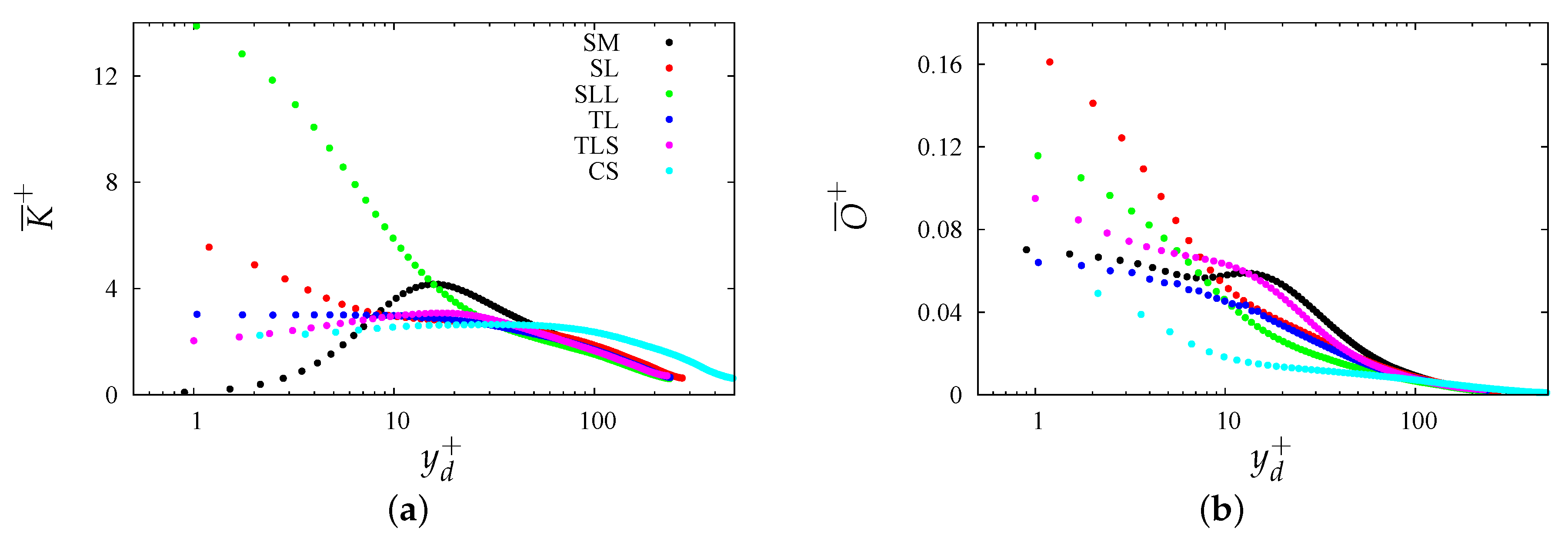
Figure 2 shows that roughness causes large modifications on both the dissipative and the energy-containing scales with respect to the case of smooth walls. In the latter case, K ¯ has a maximum at y d + 15 (where y d is the distance from the plane of the crests), and it is zero at the wall, whereas large values are observed at the plane of the crests for rough surfaces. In the case of the T L S triangular bars and of three-dimensional corrugations ( C S ), K ¯ increases slowly with the distance from the wall. In the case of the T L bars, K ¯ + is nearly constant near the plane of the crests. On the other hand, in the case of square bars, the maximum of K ¯ is at the plane of the crests, and K ¯ decreases moving towards the interior of the pipe. In the case of the S L L corrugations, intense velocity fluctuations in the wide groove between the two bars yield large value of the maximum of K ¯ .
The size, location, and shape of the energy-containing scales cannot be appreciated from the radial profiles only. However, all profiles in Figure 2a, with the exception of the C S case, are superposed in the outer region. The same coincidence is observed for the profiles in outer units only for corrugations with similar values of wall friction, namely S M , T L , and T L S . Some small difference is observed for the S L corrugation, whereas for the C S geometry, which has large drag, K ¯ in the outer region is higher that for the smooth case. At low Reynolds number, the good collapse in wall units indicates strong connection between friction and turbulence. Details on the shape, and on the interaction among the energy-containing structures, may be inferred by large-scale eduction procedures, as those introduced by Jimenez [15]. The eduction of the coherent structures is rather complex in two-dimensional channels, and the computational effort in circular pipes and in the presence of rough walls further increases. Preliminary insight into the interaction among the flow structures may be obtained through contours plots of K ^ = v i v i ^ / 2 in planes orthogonal to the flow direction, with v i = V i V ^ i . The hat symbol here indicates averages in the streamwise direction, and in time.
Before analyzing the distribution of the energy-containing scales, it is worth showing the radial distributions of the dissipative scales, depicted through O ¯ + in Figure 2b. For all kinds of surfaces, the maximum of O ¯ + occurs at the plane of the crests and O ¯ + decays moving towards the central part of the pipe. The bump occurring y d + > 8 for the smooth pipe case, and due to the interaction between ribbon- and rod-like structures, is barely appreciable for the T L S geometry. Letting S ¯ = s i j s j i ¯ , it is worth recalling that, if S ¯ > O ¯ , the small-scale structures are ribbon-like, whereas rod-like structures are found in the opposite case. For all the other corrugations, the enstrophy decays monotonically, starting from y d + 20 , at different rates. With the exception of the C S case, the profiles of O ¯ + collapse in the core region. For the C S geometry, large values of O ¯ occur at any wall distance (as for K ¯ ), whereas values for the S L geometry are slightly higher than for the other geometries. The large values of O ¯ for the C S , S L , and S L L geometries are associated with intense vorticity generation at the corners of the longitudinal bars or of the cubic elements. The formation of high values of K ¯ and of O ¯ for C S can be appreciated from the plots in Figure 2 by considering that, in Table 1, Re τ for the C S case is three times higher than for the other corrugations.

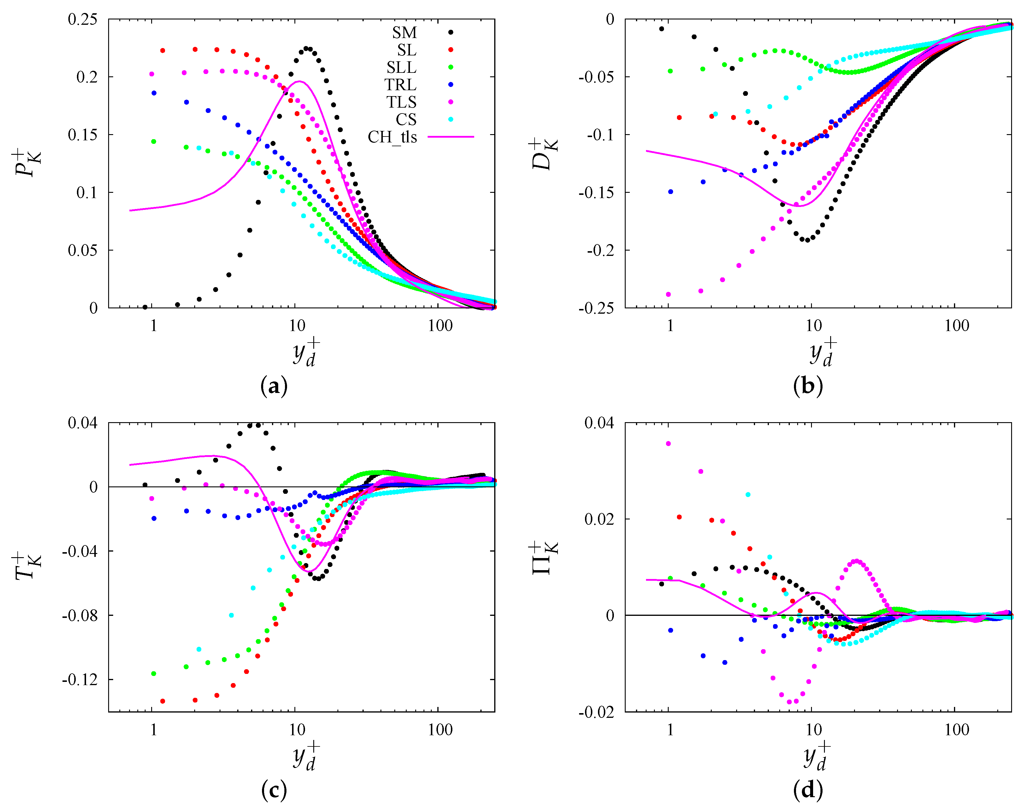
3.2. Budgets of Turbulence Kinetic Energy

The budget of the turbulence kinetic energy highlights the contribution of production, rate of dissipation, and transfer in space. In the presence of smooth walls, the effect of the first two terms is felt in all regions of the duct, whereas transfer is only comparable in the near-wall region. In two-dimensional rough channels, Orlandi [14] showed dependence of each term on the type of surface. It is then worth establishing whether the same behavior also holds in circular ducts. In this respect, we wish to recall that budgets are traditionally obtained from the Navier–Stokes equations, by averaging along the streamwise and spanwise directions and in time, leading to the equations for the mean velocity components V ¯ i , the subscript i indicating the radial (r), azimuthal ( θ ), and axial (z) directions. Transport equations for the fluctuating velocity components v i are then obtained by subtracting from the equations for the instantaneous velocity field V i = V ¯ i + v i the V ¯ i equations. Summing the equations for v i multiplied by the respective velocity fluctuations yields a transport equation for the squared velocity fluctuations K = ( v r 2 + v θ 2 + v z 2 ) / 2 , which averaged in time and in the homogeneous directions yield the transport equation for K ¯ = ( v r v r ¯ + v θ v θ ¯ + v z v z ¯ ) / 2 ,
0 = C K v r v z ¯ d V z ¯ d r P K d v r K d r ¯ T K v r p r ¯ + Π K
1 R e v z 2 v z ¯ + v θ 2 v θ ¯ + v r 2 v r ¯ + 1 r 2 v θ v θ ¯ v r v r ¯ + 2 v θ v r θ ¯ v r v θ θ ¯ D K
The condition V r ¯ = 0 sets the convective term C K = V r ¯ K ¯ r to zero. The turbulent transfer term T K accounts for the triple velocity correlations, Π K for the pressure–velocity gradient correlations, P K is the production term and D K is the total dissipation. Note that here the latter term is not split into viscous diffusion and isotropic dissipation, as traditionally done. Orlandi [14] pointed out that this simplification may lead to advantages in RANS closures for flows past smooth and rough walls. Qualitative comparison between the budgets in Figure 12 of Orlandi [14] for channels and those in Figure 3 shows similar trends, with the exception of the T L S geometry, which in the case of channels yields slight drag reduction, whereas here it yields a slight drag increase.
In the case of a smooth pipe, all the terms (black solid circles) in Figure 3 are zero at the wall, and dissipation nearly balances production everywhere in the pipe. The energy transfer term T K marks the imbalance between P K and D K in the buffer layer, with a positive maximum in the region where ribbon- and rod-like structures interact. Orlandi [14] stressed that the prevalence of one on the other kind of structure may be detected in the profiles of d 2 v r v r ¯ / d r 2 , which change signs almost at the same distance from the wall as T K .
In the case of rough surfaces, the production term is approximately constant in a thin layer near the plane of the crests, with values between 0.15 and 0.22 , which do not differ much from the smooth wall case. Hence, it may be stated that proportionality between production and friction holds. For instance, the peak production for the C S case would be a factor twenty higher than the smooth case, which is close to the ratio of the scaling factors ( 1 / ( u τ 4 R e ) ) for the two surfaces. For the S L geometry, production is 2.7 times that of the smooth case, again close to the ratio between the scaling factors. For the other types of corrugations, the occurrence of similar values of Re τ implies that the maximum production at the plane of the crests equals the peak value in the smooth case. For the T L S geometry, the different behavior of production in pipe (solid magenta circle), and channels flow (solid magenta line) allows for understanding drag reduction in the channel. In fact, P k = τ V τ R Re , and in pipe at the plane of the crests, we have τ R τ V , whereas in the channel flow (see Table 1 in Orlandi [14]), one has τ R < τ V . In addition, the maximum of P K does not occur at the plane of the crests for the channel. To be more clear, drag reduction is achieved when the velocities at the plane of the crests reduce τ V more than the increase of τ R . This effect was investigated in detail by DiGiorgio et al. [31].
As previously mentioned for the S M geometry, the rate of total dissipation D K (see panel (b)) balances production ( P K ) rather well. On the other hand, imbalance between P K and D K is clear for the other corrugations, and in particular for the C S , S L L , and S L geometries. The negligible contribution of Π K (see panel (d)) implies that the imbalance between P K and D K is equilibrated by T K . This is in fact conveyed in panel (c), which shows large T K for S L , C S , and S L L , near the plane of the crests. In the case of triangular bars, the intensity of the ejections from the interior of the corrugation, quantified in terms of v r v r ¯ | w in Table 1, decreases, yielding small values of T K . In Table 1, one can see that v r v r ¯ | w is almost ten times higher for the C S geometry than for any other surface, implying large eruptions from the interior of the cubes, and large values of the budget terms, when expressed in outer units. However, Figure 3 shows that, when expressed in wall units, all budget terms for the C S geometry are comparable to the other geometries, implying that the balance of the turbulence kinetic energy is strictly linked to drag mechanisms.
To appreciate the previous discussion in greater detail, it is worth analyzing the distribution of the turbulence statistics in the cross-stream plane, without averaging along the azimuthal direction, which allows for uncovering the presence of secondary motions.

3.3. Definition of Secondary Flow

Secondary motions in time-developing flows are investigated here by evaluating the statistics in terms of the triple splitting introduced by Hussain and Reynolds [10]. Those authors applied the decomposition to the time signals of hot-wire probes. Here, coherent motions are identified from averages of the flow variables in the streamwise direction (denoted with the hat symbol, · ^ ), and in time (denoted with angle brackets, · ), e.g., v ^ i . Their azimuthal averages (denoted with the tilde symbol, · ˜ ) yield the standard Reynolds averaged profiles, e.g., v ^ i ¯ . Deviations of the time and streamwise averaged fields with respect to the Reynolds averages are denoted with the tilde symbol ( · ˜ ), and referred to as coherent fluctuations, hence
v ˜ i = v ^ i v ^ i ¯ .
Fluctuations with respect to the time and streamwise average fields are indicated with a double prime and referred to as incoherent, such that
V i = v ^ i ¯ + v i = v ^ i + v i ,
The distribution of the Reynolds stresses in the r θ plane can then be expressed as
R i j ( r , θ ) = v i v j ^ = v i v j ^ + v ˜ i v ˜ j ^ = R i j ( r , θ ) + ρ i j ( r , θ ) ,
where we have accounted for the fact that coherent and incoherent fluctuations are uncorrelated. In Equation (5), the stresses R i j account for the effect of incoherent motions, and ρ i j 
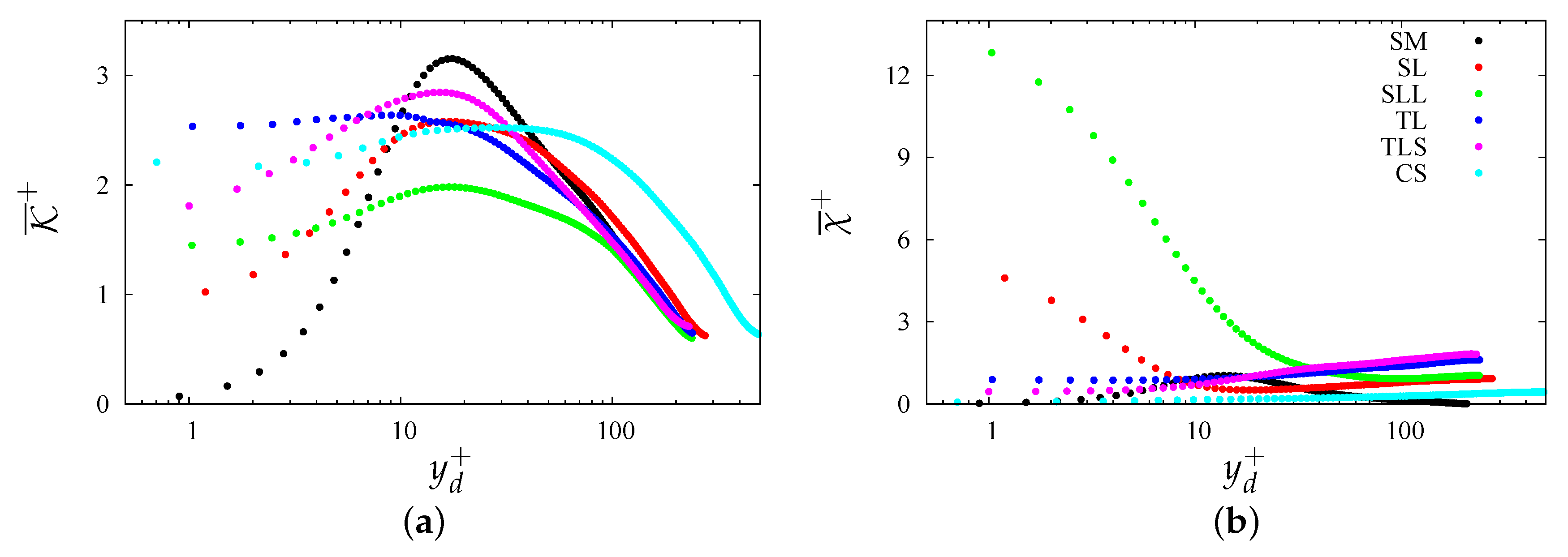
account for coherent motions. In the absence of wall corrugations, secondary motions may still be present because of the coherence of the flow structures. In the presence of wall corrugations, and, in particular for corrugations aligned with the flow direction, space coherence is expected and in some sense enforced. The turbulence kinetic energy, previously shown in Figure 2a, is split after (3), as K = K + χ , K = R i i / 2 , χ = ρ i i / 2 , indicating the contribution of incoherent and coherent motions, respectively. Their azimuthally averaged profiles, shown in Figure 4, suggest a large dependence on the type of corrugation. For the C S , T L and T L S surfaces, the coherent energy (Figure 4b) is negligible, implying that the coherent disturbances v ˜ i are small, and the incoherent disturbances emanating from the roughness are the main contributors to the turbulence kinetic energy. In the case of the C S corrugation, this is true at any distance from the plane of the crests. In the case of the triangular bars (TL, TLS), χ ¯ increases with the distance from the plane of the crests, and it becomes larger than K ¯ near the center of the pipe. In the case of smooth walls, v ˜ i reaches a maximum at a certain distance from the wall, implying that streamwise-elongated structures are coherent in space and time. However, the incoherent contribution is larger than the coherent one, at any distance from the wall. For the S L L corrugation, the coherent energy overcomes the incoherent one. Later on, we will show that this is due to the presence of intense coherent structures which are anchored to the longitudinal bars. In particular, χ decreases near the wall, and it becomes comparable to K at y d + 20 , which shows that the size of these energy-containing scales is 0.1 R c , comparable to the size of the corrugations. For S L corrugations, the peak of χ ¯ reduces with respect to the S L L case, but it is still dominant over K ¯ . The two contributions are equal at y d + 5 , to indicate that the coherent structures generated near the corner of the corrugations are smaller than the size of the square bars.

3.4. Visualization of Secondary Flows

3.4.1. Effect of Reynolds Number in Smooth Pipe

Before analyzing the effects of wall roughness on the distribution of the coherent and incoherent statistics, it is worthwhile examining the influence of the Reynolds number in the case of smooth pipe. Based on DNS data in plane channels [4,36], Orlandi [14] showed strong variation of the peak of K ¯ at low Re , and tendency to saturation at higher Re . The location of the peak of K ¯ ranges from y d + = 15 at Re τ = 78 , to y d + = 18.65 at Re τ = 5200 , implying better scaling of the energy-containing wall structures with the wall friction at high Re . Figure 5c shows that this Reynolds number dependence also holds for the circular pipe. In this figure, the lines correspond to the data of Wu and Moin [37], whose DNS (denoted as WM44 in the figure) was carried out in a L z = 15 long domain, reaching Re τ = 1150 . Figure 5c shows good agreement between the open circles, (sum of the contributions in Figure 5a,b), and the kinetic energy distribution of Wu and Moin [37]. Pirozzoli et al. [38] carried out simulations at high Reynolds number, reaching Re τ = 6000 (denoted as P285 in the figure). As in channel flow [4], the peak of K ¯ + continues to grow with the Reynolds number, whereas its location does not change, indicating that the size of the near-wall energy containing structures scales with u τ . Figure 5a,b show the Reynolds number dependence of the incoherent and coherent contributions on the turbulence kinetic energy. The coherent part is less than the incoherent one at all Re , and it decreases with Re . This splitting was not carried out for the simulations of Pirozzoli et al. [38], which would quantify the coherent contribution of the large-scale structures in the outer region. From the present moderate- Re simulations, we may infer a tendency to saturation of χ ¯ + with Re . This observation might be of interest for LES, which should be able to accurately resolve the coherent contributions. The decrease of the coherent contribution at high Re implies a smaller effect of the near-wall structures. The oscillatory motion in the azimuthal direction of the coherent structures causes slow convergence of the numerical simulations. At low Re , the size of the coherent structures is comparable to the radius of the pipe, with an effect on the entire flow. Figure 5b shows that, at Re = 6534 , χ ¯ + is one fourth of K ¯ + , and that the contribution increases at Re = 4900 . In Figure 5b, most coherent energy is distributed within y d + < 100 , with peak at a wall distance y d + 15 .

3.4.2. Effect of Wall Corrugations

The profiles of the coherent and incoherent turbulent stresses allow for understanding which of them contributes most to the turbulence kinetic energy, and in which part of the duct. The prevalence of one normal stress on the others is strictly connected to the type of corrugation. It should be pointed out that the normal stress in the flow direction ( v z v z ¯ ) is largest, being directly generated from interaction between mean shear and fluctuating statistics. The turbulent shear stress ( v r v z ¯ ) at the plane of the crests contributes to the friction of rough walls, and its distribution accounts for the turbulence kinetic energy production. In all panels of Figure 6, the coherent contributions are denoted with solid lines in the same color as in the main panel. In almost all cases, the incoherent part of the stresses prevails over the coherent one. In particular, in Figure 6a, we see a large increase of ρ ¯ z z near the plane of the crests, for the longitudinal square bars, and in particular for the S L L corrugations. Velocity visualizations reveal penetration of the external flow within the grooves, and acceleration over the bars. Near the plane of the crests, the fluctuations of V ˜ z are larger than v z , which yields ρ ¯ z z > R ¯ z z , as shown later on from their distribution in the r θ plane.
For all other normal stresses, the incoherent contribution prevails over the coherent one. For S L L corrugations, Figure 6b shows that the coherent radial stress ( ρ ¯ r r ) is larger than for the other types of corrugations, although an order of magnitude smaller than the incoherent contribution ( R ¯ r r ). The latter remains constant up to y d + 30 , implying an increase of V ˜ r in the region close to the bars. This figure also emphasizes the ejection of intense incoherent fluctuations from C S corrugations. The coherent contribution is very small also as a result of larger friction in the case of staggered cubes. Figure 6c shows that the lateral motion close to the wedges of triangular bars yields incoherent azimuthal stresses. In the presence of square bars, the lateral fluctuations are reduced, and in the case of C S corrugations, the staggered arrangement of the cubes promotes large azimuthal fluctuations. Figure 6d shows a complex radial distribution of the shear stress components ( R r z ¯ and ρ ¯ r z ) near the plane of the crests, and collapse of the profiles of R r z ¯ for y d > 0.4 for all corrugations. This is also the case of cubic corrugations ( C S ), despite the presence of intense wall-normal ejections. This is a first hint of validity of Townsend’s similarity hypothesis [19] for flows with moderate drag increase with respect to the case of smooth wall.
The large dependence of the coherent and incoherent components of turbulence kinetic energy on the type of surface corrugation noted in Figure 6 suggests closer inspection of the stress components having the largest variations, namely ρ z z , ρ r z , R z z , R r z , for the S L L , T L S , and C S surfaces, whose cross-stream contours are shown in Figure 7. In the case of smooth pipe, the incoherent axial stress is larger than the coherent one, corroborating previous observations. However, also looking back at Figure 6a, the figure depicts good spatial correspondence between the peaks of ρ z z and R z z . In addition, the figure corroborates the discussion about Figure 5, showing that coherent structures promote the azimuthal undulations of R z z , and consequently of K , at y d + 15 . In Figure 7a, contours of of ρ z z + are visible up to a certain distance from the wall, hence it is clear that, in the outer region, the axial stress comes entirely from the incoherent contribution. Undulations also persist at the pipe centerline, however on a larger scale than near the wall. In fact, the large mean axial velocity gradient near the wall yields stronger instability than that in the outer region. Reduction of the coherent contribution in smooth pipe at increasing Reynolds number was observed in Figure 5b. However, visualizations as in Figure 7b at Re = 24 , 580 (not shown) reveal that azimuthal undulations of the incoherent stresses do not disappear.
The contributions to the turbulent shear stress shown in Figure 7c,d are rather similar to the axial stresses, in particular regarding their coherent part. We previously noticed that the azimuthal location of the respective peaks match quite well, whereas the peaks of ρ r z + are at a greater distance than for ρ z z + . Here, we find better correspondence between the contours of the turbulence shear stress in Figure 7c,d, with those of the normal stresses (not shown), which further corroborates the importance of the wall-normal stress in turbulent flows past smooth and rough flows [27]. The profiles of the coherent and incoherent contributions for the T L S corrugations, in Figure 6 (magenta symbols), show a behavior similar to that of S M (black symbols), and a large difference for the incoherent part. The visualizations in Figure 7e–h clearly highlight similarities and differences with respect to the S M case (Figure 7a–d). It is important to note that, in the case of T L S corrugations, the large number of wedges generate small-scale disturbances near the plane of the crests, thus destroying the peaks of the coherent and incoherent turbulence kinetic energy found in the smooth case. In addition, in the case of T L S corrugations, we find that peaks of the turbulent shear stress are correlated with peaks of the wall-normal stress.
The statistics for S L L corrugations reported in Figure 6a,d showed contributions of the coherent stresses to be larger than for any other type of longitudinal corrugations. For instance, at the plane of the crests, we find ρ z z + 30 for S L L , and ρ z z + 11 for S L . The profiles in Figure 6 are given above the plane of the crests, hence the visualizations are displayed in the same region. The contour plots in Figure 7i–l well explain the reasons for the peculiar behavior of S L L . In Figure 6a, we see that the coherent axial stress becomes of the same order as the incoherent one at y d 0.2 , at which peaks are visible in Figure 7i–j. Within this layer, coherent stresses are larger than incoherent ones, both above the bars and within the groove. On the other hand, the incoherent axial stress contribution decreases above the center of the groove, explaining why in Figure 6a the values of R z z ¯ for 0.1 < y d < 0.2 are smaller for S L L corrugations than for the smooth case. Small patches with negative coherent shear stress (black lines) are visible in Figure 7k, which are more intense than the incoherent negative contributions in Figure 7l. In these figures, it appears that the thin black contours are emerging from the interior of the cavity and, in particular they are adjacent to layers with high R r r close to the side walls of the bars. In Figure 6d, the coherent shear stress (green line) decreases for 0.05 < y d , corresponding to the location where the incoherent shear stress starts to increase. This is corroborated from the observed prevalence of R r z on ρ r z in the central region of Figure 7k–l. In addition, it may be appreciated that the peaks of R r z occur above the bars, and they are located at a distance y d 0.3 (corresponding to about 80 wall units), where ρ r z is nearly zero.
Regarding the cubic obstacles ( C S ), which yield the largest flow resistance, Figure 6a showed strong reduction of the coherent and incoherent axial stresses, which comes with absence of yellow and red contour levels in Figure 7m,n. On the other hand, Figure 7p shows accumulation of the incoherent shear stress in regions having the same size as the cubes. Their large values at the plane of the crests implies that the high resistance is mainly due to the incoherent shear stresses. It should be recalled that, in Figure 7, stresses are expressed in wall units, and the value of u τ for C S corrugations is approximately two times higher than for the other corrugations. Returning to the case of the longitudinal square bars, we have noted that increased coherence is due to organized wall-normal disturbances taking place near the walls of the cavity. For the S L L corrugations, the disturbances are so strong as to generate wall structures larger than the height of the bars (Figure 7j,l). Similar figures for the S L corrugations (not reported) indicate that disturbances normal to the wall affect a layer of thickness h near the plane of the crests. The distributions of the stresses for y d > 0.2 are similar to those in the smooth pipe. For triangular bars, wall-normal disturbances reduce in amplitude, and the wall structures are similar to those found in the smooth case.
The wall-normal velocity disturbances were mentioned in the discussion of Figure 7, for their action of driving coherent and incoherent turbulent stresses near the plane of the crests. Hence, in Figure 8, we analyze the distributions of the coherent wall-normal velocity ( V r ^ ) for the same wall corrugations. To better understand the influence of the corrugations, in Figure 8, the contours are also shown below the plane of the crests. From a first inspection, one can identify a region with large values of V r ^ inside and near the plane of the crests, with the latter linked to the type of surface. In the central region, with the exception of S L L , the flow structures are similar to those found in the smooth case. This is well depicted for the T L S corrugations in Figure 8b by the thin blue region with negative radial velocity near the edge of the triangles, and positive radial velocity inside the grooves. For C S corrugations, the radial velocity is non-zero at all points under the plane of the crests, on account of motion within the staggered cubes. For the S L L corrugations, the distance between any two bars is comparable to the pipe radius, hence the size of the patches with non-zero radial velocity is comparable to that in the central region. This figure may be regarded as a visual proof of Townsend’s similarity hypothesis, previously discussed in Figure 6. In fact, disturbances emerging from the wall corrugations affect a layer of about one or two roughness thicknesses. In the outer region, the flow structures are similar to the smooth case, and their size is of the order of the pipe radius.

3.5. Budgets of Secondary Turbulence Kinetic Energy

The geometry of the wall corrugations affects the coherent and incoherent contributions to the turbulence kinetic energy in the wall region, as shown in Figure 4. The effect of the type of wall corrugation can then be further explored by evaluating the budgets of K ¯ and χ ¯ . For that purpose, a transport equation for the incoherent kinetic energy ( K ) is derived,
K t = C ^ r θ + P ^ r θ + T ^ r θ + Π ^ r θ + D ^ r θ ,
where K / t = 0 if the average is done over a sufficient number of flow samples. The convective term is
C ^ r θ = v r ^ K r + v θ ^ r K θ ,
and the production term is
P ^ r θ = R r z v z ^ r + R r r v r ^ r + R r θ v θ ^ r + 1 r R θ z v z ^ θ + R θ r v r ^ θ + R θ θ v θ ^ θ + v θ ^ R θ r + v r ^ R θ θ ,
turbulent diffusion due to the triple correlation is
T ^ r θ = 1 2 r r ( v r v r v r ^ + v θ v θ v r ^ + v r v z v z ^ ) r + ( v θ v r v r ^ + v θ v θ v θ ^ + v z v z v θ ^ ) θ ,
turbulent diffusion due to the pressure–velocity correlation is
Π ^ r θ = 1 r p v r ^ r r + p v θ ^ θ ,
and the total dissipation is
D ^ r θ = 1 R e v θ 2 v θ ^ R θ θ r 2 + 2 v θ r 2 v r θ ^ + v r 2 v r ^ R r r r 2 2 v r r 2 v θ θ ^ + v z 2 v z ^ ,
each of these terms varying both in θ and r. Averaging along the azimuthal direction yields
K ¯ t = C ^ r θ ¯ + P ^ r θ ¯ + T ^ r θ ¯ + Π ^ r θ ¯ + D ^ r θ ¯ .
A budget equation for the azimuthally averaged coherent turbulence kinetic energy χ ¯ (shown in Figure 4b) is also derived, by expressing each term in Equation (2) in terms of the v i velocity fluctuations, after Equation (4), thus obtaining
χ ¯ t = C ˜ r θ ¯ + P ˜ r θ ¯ + T ˜ r θ ¯ + Π ˜ r θ ¯ + D ˜ r θ ¯ .
As an example, the procedure applied to the production term, P K = v i v j ^ V ¯ i x j in Equation (2) yields
v i v j ^ V ¯ i x j = R i j V ^ i x j + R i j V ˜ i x j + ρ i j V ¯ i x j + v i V ˜ j ^ V ¯ i x j + v j V ˜ i ^ V ¯ i x j .
The azimuthal average of the last two terms is zero, hence the coherent component of the production term comes from the second and third terms on the right-hand side of Equation (14). The same procedure allows for evaluating the coherent contribution to each term of the budget.
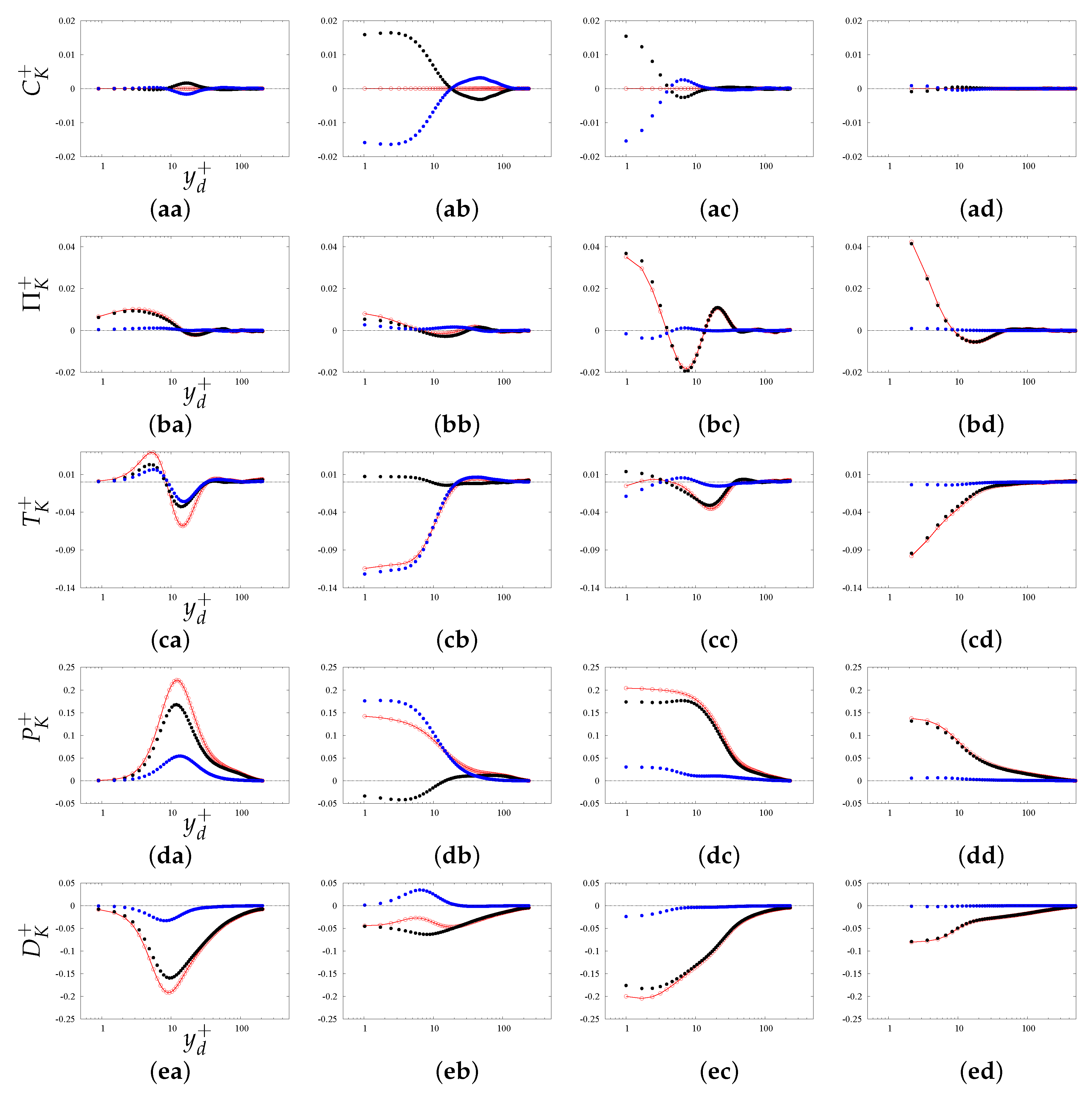
The profiles of each term of the budget in Equation (2), split into incoherent (Equation (12)) and coherent (Equation (13)) parts are depicted in Figure 9, for the wall corrugations discussed in Figure 7. In Figure 9, the solid red lines indicate the profiles of each term in Equation (2), the solid black points to those of Equation (12), and the blue solid circles those in Equation (13). The sum of the latter two contributions, indicated with the open circles, indeed coincides with the solid line. The same vertical range is used for all corrugations, to better appreciate the impact of the wall geometry. The top row shows that the convective term is nearly zero for all corrugations, due to the balance between the incoherent ( C ^ r θ ¯ ) and the coherent ( C ˜ r θ ¯ ) contributions. For the smooth pipe, the peak location of the latter term is close to the point of maximum production, which coincides with the center of the structures, as shown in Figure 7c. The peaks occur at the plane of the crests for the S L L (Figure 9ab), and for the T L S corrugations (Figure 9ac), and are much larger than for a smooth pipe. In the case of triangular bars and staggered cubes C ^ r θ ¯ , and hence C ˜ r θ ¯ decays sharply to low values, implying the formation of small secondary structures, as is clear in Figure 7 and Figure 8. The larger number of contour levels of V r ^ + in Figure 8b with respect to Figure 8d (the same also holds for V θ ^ + , not shown) explains why the maximum in Figure 9ac is larger than in Figure 9ad. For the S L L corrugations, the two contributions have a cross-over farther from the plane of crests than for any other surfaces, which is also linked to the shape of the coherent structures. This is corroborated by comparing the maps of R r z in the fourth column of Figure 7.
The panels in the second row of Figure 9 show a modest contribution of Π K to the turbulence kinetic energy budget. For all types of corrugations, the coherent contribution is negligible with respect to the incoherent one, implying rather good correlation between incoherent pressure and vertical velocity fluctuations. Hence, we may argue that in RANS closures it is reasonable to neglect this term, or incorporate its contribution into the turbulent transfer term. The profiles of T K , shown in the third row of Figure 9, highlight different behavior of smooth and corrugated pipes, as in the latter case turbulent transfer may become of the same order of magnitude as production. Looking at Equation (9), we see that turbulent transfer includes derivatives of triple correlations in the azimuthal direction, which yield zero contribution when averaged in θ , and in the radial directions. Among the first three terms on the right-hand side of Equation (9), the largest is associated with the v r v z v z ^ correlation, supporting the important role of the wall-normal velocity fluctuations, which are most intense for the S L L corrugations, as shown in Figure 8. In that case, the coherent contribution dominates over the incoherent one. In the case of staggered cubes, Figure 9cd shows large values of the total T K + as those for S L L corrugations. The incoherent contribution prevails in the case of staggered cubes, whereas the coherent contribution is dominant in the case of S L L corrugations. The magnitude of the turbulent transfer is similar for triangular bars (Figure 9cc) and smooth pipes (Figure 9ca), the coherent transfer is negligible for the T L S corrugations, whereas coherent and incoherent contributions do not differ much in the smooth case.
The incoherent production term as defined in Equation (8) accounts for interaction between the velocity gradients associated with large flow scales, and the fluctuating velocity correlations associated with small turbulence scales. For rough walls, the overall production term (red in Figure 9) is different from the case of smooth walls, and it strongly depends on the geometry of wall corrugation, with coherent and incoherent contributions having much different relative importance. Similarity of coherent and incoherent contributions to production implies similarity of the shape of the wall structures, which however differ in strength, as seen in Figure 7c,d. The relative magnitude of the coherent and incoherent production for triangular bars ( T L S , see Figure 9dc) is similar to the smooth case (see Figure 9da). However, their profiles differ, as for in the smooth case P K + has peak at y d + 15 , and it is zero at the wall, whereas, in the T L S corrugations, the peak occurs near the plane of the crests, in agreement with the visualizations in Figure 7h. The production term for staggered cubes corrugations is similar and smaller than for the triangular bars, but the coherent contribution is negligible for C S . In the case of the S L L corrugations (Figure 9db), coherent and incoherent production have opposite signs, the former being larger than the latter in magnitude.
As discussed in Figure 3a,b, production and dissipation are nearly locally balanced for smooth pipes. The bottom panels in Figure 9 show that this is also the case for their coherent and incoherent contributions. On the other hand, in the case of the S L L corrugations, the profiles of production (Figure 9db)and dissipation (Figure 9eb) are quite different, because of the relevant role of the turbulent transfer term (Figure 9cb). In that case, dissipation is generally smaller than production, and Figure 9eb shows that the incoherent contribution is larger in magnitude than the coherent one, which yield a negative contribution. Hence, we may argue that the coherent contribution generates coherent energy that is transferred into the interior of the pipe through coherent turbulent diffusion.
The profiles of the turbulence kinetic energy budget terms in Figure 9 highlight a more complex behavior for the S L L corrugations than for the other types of corrugations. Hence, in Figure 10, we show in detail the behavior of each term of the total, incoherent, and coherent contributions. The data reported in Figure 3 are repeated in Figure 10a to better understand the relative contribution of the various terms. Figure 10a shows that the convective term and the pressure–velocity transfer term do not contribute to the budget. The production term in the wall region is transferred to a large extent towards the outer region through turbulent transport. The local rate of dissipation is rather small in the wall region, and it tends to balance production in the outer region. The terms of the incoherent kinetic energy budget shown in Figure 10b are smaller than the respective terms in the coherent budget, shown in Figure 10c. Transfer, convective, and the pressure–velocity terms are negligible in the incoherent budget. Near the plane of the crests production is negative, and it removes the same amount of incoherent energy as directly dissipated. The two terms together yield a negative imbalance (black line), which is also reported as the red line in Figure 10d. This imbalance is compensated by positive imbalance in the budget of the coherent kinetic energy energy, namely the blue line in Figure 10d. The latter term comes from the budget profiles in Figure 10c, where it is interesting to notice a peculiar positive dissipation.
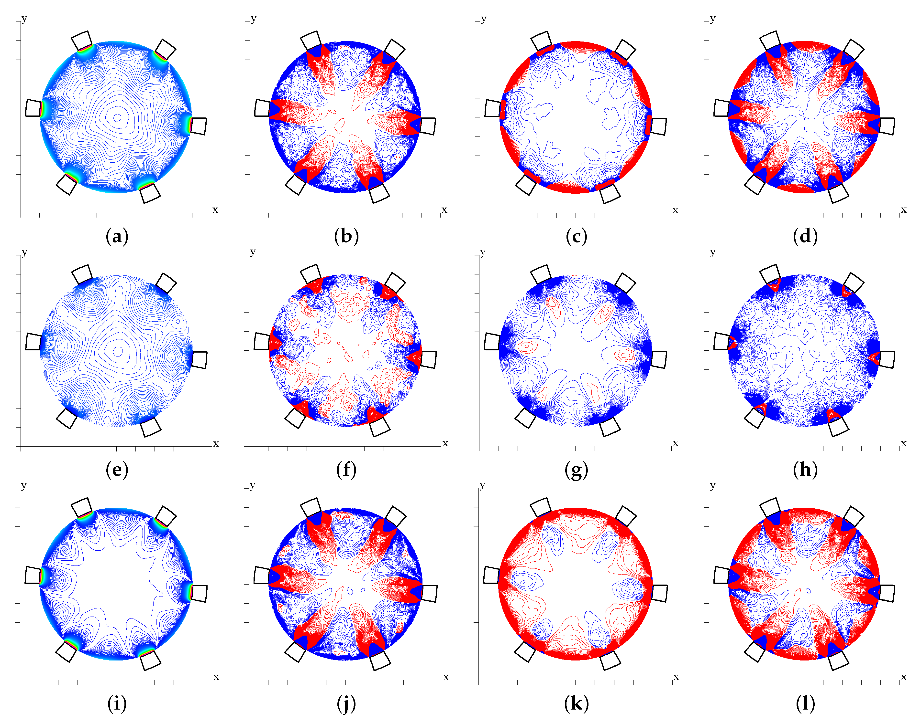
In the S L L corrugations, the roughness elements are spaced a distance w / k 5 apart, hence flow around any longitudinal bar does not directly affect the other. The formation of intense coherent structures allows for understanding the flow modifications near one element, leading to the azimuthal non-uniform distribution of the coherent and incoherent contributions to each term of the budgets. In the first column of Figure 11, we show the distributions of the turbulence kinetic energy K (Figure 11a), and of its incoherent K (Figure 11e) and coherent χ (Figure 11i) contributions. The latter two fields are similar to those of the streamwise stress reported in Figure 7i,j, as the axial stresses dominates over the radial and azimuthal ones. The budgets in Figure 10 showed dominant contribution of production and turbulent transfer to the coherent budget. The contour plots of the total dissipation distributions in the cross-stream plane (not reported) indicate that they are mainly concentrated in thin layers near the plane of the crests, with values smaller than the production terms. Strong azimuthal non-uniformity of the terms in the budget of coherent turbulence kinetic energy and dissipation terms ( P ˜ + D ˜ ) in Figure 11k, and the other terms ( T ˜ + C ˜ + Π ˜ ) in Figure 11j. In Figure 11j, we see that the negative contribution in proximity of the grooves cavities prevails over the positive contribution near the bars, with the final result of transfer of coherent kinetic energy from the plane of the crests towards the central region. This is corroborated by the contours of the coherent radial velocity in Figure 8c, which indicated organized radial flow towards the center of the pipe. The sum of all terms in the coherent kinetic energy budget (shown in Figure 11l) is generally positive, to indicate that the positive transfer around the bars prevails on the negative contribution from production and dissipation, and vice versa in the region above the cavity. Azimuthally averaging the budget sum in Figure 11l yields the positive profile (blue line) in Figure 10d. The distribution of the overall incoherent budget in Figure 11h is negative almost everywhere, with the exception of a small positive region above the bars. Despite large differences between Figure 11l and Figure 11h, their azimuthal averages have similar radial distribution, with the opposite sign as reported in Figure 10d. The contours of the incoherent kinetic energy production (not shown) depict two negative patches near square bars, and positive values above. The incoherent rate of dissipation is negative in any region, hence in Figure 10d the sum of production and dissipation becomes more negative close to the bars. Dissipation is rather small above the bars, hence positive production is responsible for the observed positive patches above the bars. The azimuthal average of the positive and negative transfer terms in Figure 11f leads to the small values in Figure 10b. The red spot of the transfer term above the bars is a magnitude larger than the sum of production and dissipation (which is negative), hence red spots are also visible in the budget sum in Figure 11h. The visualizations of the coherent and incoherent budgets distributions and of the coherent and incoherent components of the turbulence kinetic energy allow for understanding the dominance of either term in the budget of the overall kinetic energy, which are shown in the top panels of Figure 11. It may be concluded that, for S L L corrugations, the coherent contribution prevails over the incoherent one. This is particularly true for the turbulent transfer, as inferred from similarity between Figure 11b and Figure 11j. Local imbalance between production and dissipation is affected by the roughness elements, which leads to zones with production locally exceeding dissipation, and regions near corners with dissipation excess. Turbulent transfer is the dominant term in the overall budget, and in fact its distribution in Figure 11b is similar to the budget sum in Figure 11d. The turbulence kinetic energy produced in the center of the grooves is transferred towards the corners, where it is dissipated, and part of the energy residing above the bars is transferred towards the central region.

4. Conclusions

We have performed DNS of turbulent flow in circular pipes with smooth and corrugated walls, with the size of the roughness elements one order of magnitude less than the pipe radius. Fully rough flows are then generated with a structure much different than in smooth pipes. In the past, large efforts were directed to studying similar corrugations in channels, where spanwise confinement may have an influence on the large structures residing away from the wall. In addition, geometry dictates differences between the large turbulence structures in the pipe core, and those close to the centerline of channels with rough elements on both walls. In circular pipes, the domain size in the azimuthal direction is natural, hence outer structures only change as a result of the imposed Reynolds number. Hence, it may be asserted that this is the most suitable set-up to analyze interactions between the near-wall structures and those occurring at the center of the pipe. In plane channels, one-dimensional spectra have been used to gain information regarding the flow structures above the plane of the crests, and to describe the complex turbulence kinetic energy budget [8]. Extension of that analysis to circular pipes would be rather complex, due to the appearance of several extra terms. Here, the analysis is carried out in physical space, leveraging on decomposition of the velocity field to isolate coherent and incoherent motions, defined in terms of their persistence in the axial direction. This procedure has been seldom used, and we believe it to be particularly appropriate in the presence of wall corrugations.
In the case of smooth walls, we have found that coherent motions are especially significant in the wall region at low Reynolds numbers, whereas their amplitude increases far from the wall at a higher Reynolds number. This is an important point to be investigated, and we plan to use recent DNS data [38] to investigate the growth of the amplitude of the coherent structures in the outer region. This would allow for shedding some light on the still open debate about the connection and interaction between near-wall and outer-layer structures.
All terms in the turbulence kinetic energy budget have been evaluated for several types of wall corrugations, and we have found that those are distributed quite differently than in flows past smooth walls. In particular, three-dimensional corrugations made up of staggered cubes can generate strong disturbances which affect a fluid layer with thickness similar to the size of the cubes. For this type of corrugations, coherent motions are weaker than incoherent ones. Irrelevance of the coherent motion is also observed for contiguous triangular corrugations, due to small-scale disturbances generated inside the grooves. Coherent motions in the presence of square bar corrugations are found to dominate over incoherent ones, owing to strong disturbances created by the flow in the groove between adjacent bars. Increasing the gap between the bars, coherent motions become relatively even more important than the incoherent ones. This kind of corrugation has been investigated in detail, leading to the conclusion that, near the plane of the crests, the production of incoherent turbulence kinetic energy is negative, whereas the coherent dissipation is locally positive. For this type of corrugation, turbulent transfer is found to be comparable with production. We have also observed that imbalance of the coherent budget terms is perfectly compensated by imbalance of the incoherent budget terms. The above conclusions have been verified under low Reynolds number conditions, hence it would be important to verify whether our conclusions can also be extended to higher Reynolds numbers.

Author Contributions

Conceptualization, P.O. and S.P.; software, P.O.; formal analysis, P.O.; writ- ing—original draft preparation, P.O.; writing—review and editing, S.P. All authors have read and agreed to the published version of the manuscript.

Funding

This research received no external funding.

Institutional Review Board Statement

Not applicable.

Informed Consent Statement

Not applicable.

Data Availability Statement

No external data reported.

Acknowledgments

The authors acknowledge fruitful discussions with Simone Di Giorgio. We also acknowledge that some of the results reported in this paper have been achieved using the PRACE Research Infrastructure resource MARCONI based at CINECA, Casalecchio di Reno, Italy.

Conflicts of Interest

The authors have no conflict of interest to disclose.

References

  1. Hussain, A.; Reynolds, W. The mechanics of an organized wave in turbulent shear flows. Part. 2. Experimental results. J. Fluid. Mech. 1972, 54, 241–261. [Google Scholar] [CrossRef]
  2. Hoyas, S.; Jimenez, J. Scaling of the velocity fluctuations in turbulent channels up to Reτ = 2003. Phys. Fluids 2006, 18, 011702. [Google Scholar] [CrossRef] [Green Version]
  3. Kim, J.; Moin, P.; Moser, R. Turbulence statistics in fully developed channel flow at low Reynolds number. J. Fluid Mech. 1987, 177, 133–166. [Google Scholar] [CrossRef] [Green Version]
  4. Lee, M.; Moser, R. Direct simulation of turbulent channel flow layer up to Reτ = 5200. J. Fluid Mech. 2015, 774, 395–415. [Google Scholar] [CrossRef]
  5. Reynolds, O. On the dynamical theory of incompressible viscous fluids and the determination of the criterion. Philos. Trans. R. Soc. 1895, 186, 123–164. [Google Scholar]
  6. Laufer, J. The Structure of Turbulence in Fully Developed Pipe Flow; NACA TR 1174; National Bureau of Standards: Washington, DC, USA, 1954; pp. 1–18. Available online: https://ntrs.nasa.gov/api/citations/19930092199/downloads/19930092199.pdf (accessed on 1 December 2021).
  7. Hoyas, S.; Jimenez, J. Reynolds number effects on the Reynolds-stress budgets in turbulent channels. Phys. Fluids 2008, 20, 101511. [Google Scholar] [CrossRef] [Green Version]
  8. Lee, M.; Moser, R. Spectral analysis of the budget equation in turbulent channel flows at high Reynolds number. J. Fluid Mech. 2018, 860, 886–938. [Google Scholar] [CrossRef] [Green Version]
  9. Vanderwel, C.; Ganapathisubramani, B. Effects of spanwise spacing on large-scale secondary flows in rough-wall turbulent boundary layers. J. Fluid Mech. 2015, 774, R2. [Google Scholar] [CrossRef] [Green Version]
  10. Hussain, A.; Reynolds, W. The mechanics of an organized wave in turbulent shear flows. J. Fluid. Mech. 1970, 42, 241–258. [Google Scholar] [CrossRef]
  11. Yuan, J.; Piomelli, U. Roughness en on the Reynolds stress budgets in near-wall turbulence. J. Fluid Mech. 2014, 760, R1. [Google Scholar] [CrossRef]
  12. Chan, L.; MacDonald, M.; Chung, D.; Hutchins, N.; Ooi, A. Secondary motion in turbulent pipe flow with three-dimensional roughness. J. Fluid Mech. 2018, 854, 5–33. [Google Scholar] [CrossRef]
  13. Anderson, W.; Barros, J.M.; Christensen, K.T.; Awasthi, A. Numerical and experimental study of mechanisms responsible for turbulent secondary flows in boundary layer flows over spanwise heterogeneous roughness. J. Fluid Mech. 2015, 768, 316–347. [Google Scholar] [CrossRef]
  14. Orlandi, P. Turbulent kinetic energy production and flow structures in flows past smooth and rough wall. J. Fluid Mech. 2019, 866, 897–928. [Google Scholar] [CrossRef]
  15. Jimenez, J. Coherent structures in wall-bounded turbulence. J. Fluid Mech. 2018, 842, P1. [Google Scholar] [CrossRef] [Green Version]
  16. Nikuradse, J. Laws of Flow in Rough Pipes; Technical Memorandum 1292; NASA TM; National Advisory Committee for Aeronautics: Washington, DC, USA, 1950. [Google Scholar]
  17. Hultmark, M.; Vallikivi, M.; Bailey, S.C.C.; Smits, A.J. Logarithmic scaling of turbulence in smooth- and rough-wall pipe flow. J. Fluid Mech. 2013, 728, 376–395. [Google Scholar] [CrossRef] [Green Version]
  18. Moody, L.F. Friction factors for pipe flows. Trans. ASME 1944, 66, 671–684. [Google Scholar]
  19. Townsend, A.A. The Structure of Turbulent Shear Flows, 2nd ed.; Cambridge University Press: Cambridge, UK, 1976. [Google Scholar]
  20. Kunkel, G.; Allen, J.; Smits, A.J. Further support for Townsend’s Reynolds number similarity hypothesis in high Reynolds number rough-wall pipe flow. Phys. Fluids 2007, 19, 0551009. [Google Scholar] [CrossRef]
  21. Langelandsvik, L.; Kunkel, G.; Smits, A.J. Flow in a commercial steel pipe. J. Fluid Mech. 2007, 595, 323–339. [Google Scholar] [CrossRef] [Green Version]
  22. Schlichting, H. Experimental Investigation of the Problem of Surface Roughness; NACA TM 823; National Advisory Committee for Aeronautics: Washington, DC, USA, 1936. [Google Scholar]
  23. Leonardi, S.; Orlandi, P.; Smalley, R.J.; Djenidi, L.; Antonia, R.A. Direct numerical simulations of turbulent channel flow with transverse square bars on the wall. J. Fluid Mech. 2003, 491, 229–238. [Google Scholar] [CrossRef] [Green Version]
  24. Orlandi, P.; Leonardi, S. DNS of turbulent channel flows with two- and three-dimensional roughness. J. Turbul. 2006, 7, N53. [Google Scholar] [CrossRef]
  25. Flack, K.; Schultz, M. Review of Hydraulic Roughness Scales in the Fully Rough Regime. J. Fluids Eng. 2010, 132, 041203. [Google Scholar] [CrossRef] [Green Version]
  26. Orlandi, P.; Leonardi, S.; Tuzi, R.; Antonia, A. DNS of turbulent channel flow with wall velocity disturbances. Phys. Fluids 2003, 15, 3497–3600. [Google Scholar] [CrossRef]
  27. Orlandi, P. The importance of wall-normal Reynolds stress in turbulent rough channel flows. Phys. Fluids 2013, 25, 110813. [Google Scholar] [CrossRef]
  28. Durbin, P. Near-wall turbulence closure modeling without damping functions. Theor. Comput. Fluid Dyn. 1991, 3, 1–13. [Google Scholar]
  29. Pirozzoli, S.; Modesti, D.; Orlandi, P.; Grasso, F. Turbulence and secondary motions in square duct. J. Fluid Mech. 2018, 840, 631–655. [Google Scholar] [CrossRef] [Green Version]
  30. Orlandi, P.; Pirozzoli, S. Transitional and turbulent flows in rectangular ducts: Budgets and projection in principal mean strain axes. J. Turbul. 2020, 21, 286–310. [Google Scholar] [CrossRef]
  31. DiGiorgio, S.; Leonardi, S.; Pirozzoli, S.; Orlandi, P. On the relationship between drag and vertical velocity fluctuations in flow over riblets and liquid infused surfaces. Int. J. Heat Fluid Flow 2020, 86, 108663. [Google Scholar] [CrossRef]
  32. Sassun, D.; Flores, O.; Orlandi, P. Analysis and comparison between rough channel and pipe flows. J. Phys. Conf. Ser. 2016, 708, 012011. [Google Scholar] [CrossRef]
  33. Orlandi, P.; Fatica, M. Direct simulations of a turbulent pipe rotating along the axis. J. Fluid Mech. 1997, 343, 43–72. [Google Scholar] [CrossRef]
  34. Fadlun, E.A.; Verzicco, R.; Orlandi, P.; Mohd-Yusof, J. Combined immersed boundaries finite-difference methods for three dimensional complex flow simulations. J. Comput. Phys. 2000, 161, 35–60. [Google Scholar] [CrossRef]
  35. Orlandi, P.; Modesti, D.; Pirozzoli, S. DNS of turbulent flows in ducts with complex shape. Flow Turbul. Combust 2018, 100, 1063–1079. [Google Scholar] [CrossRef]
  36. Bernardini, M.; Pirozzoli, S.; Orlandi, P. Velocity statistics in turbulent channel flow up to Reτ=4000. J. Fluid Mech. 2014, 742, 171–191. [Google Scholar] [CrossRef] [Green Version]
  37. Wu, X.; Moin, P. A direct numerical simulation study on the mean velocity characteristics in turbulent pipe flow. J. Fluid Mech. 2008, 608, 81–112. [Google Scholar] [CrossRef]
  38. Pirozzoli, S.; Romero, J.; Fatica, M.; Verzicco, R.; Orlandi, P. One-point statistics for turbulent pipe flow up to Reτ≈6000. J. Fluid Mech. 2021, 926, A28. [Google Scholar] [CrossRef]
Figure 1. Sketch of roughness geometries in a cross-stream plane with 1.2 < x < 1.2 and 1.2 < u < 1.2 : (a) S M ; (b) S L ; (c) S L L ; (d) T L ; (e) T L S ; (f) the C S geometry is depicted in a z θ ( 0 < x = θ < 2 π and 0 < z < 8 ) shell at the plane of the crests.
Fluids 06 00448 g001
Figure 2. Inner-scaled profiles of turbulence kinetic energy (a) and enstrophy (b) at Re = 6534 , for the roughness geometries given in the legend of panel (a).
Fluids 06 00448 g002
Figure 3. Terms in the turbulence kinetic energy budget (Equation (2)): (a) production ( P K + ), (b) total dissipation ( D K + ), (c) turbulent transport ( T K + ), and (d) pressure transport ( Π K + ), for the corrugations given in the legend of panel (a). C H t l s refers to data for the T L S geometry in channel flow.
Fluids 06 00448 g003
Figure 4. Profiles of (a) turbulence kinetic energy ( K ¯ ); and (b) its coherent contribution ( χ ¯ ), for the wall corrugations given in the legend ( Re = 6534 ).
Fluids 06 00448 g004
Figure 5. Flow in smooth pipes (SM): profiles of (a) incoherent turbulence kinetic energy ( K ¯ ), (b) coherent kinetic energy ( χ ¯ ), and (c) their sum ( K ¯ ), at the Reynolds numbers in the legend.
Fluids 06 00448 g005
Figure 6. Profiles of incoherent stresses R i j ¯ (symbols)(, and of the coherent stresses ρ ¯ i j (lines) in wall units versus distance y d from the plane of the crests, for the corrugations indicated in the legend of Figure 4b: (a) axial, (b) radial, (c) azimuthal, and (d) shear stress.
Fluids 06 00448 g006
Figure 7. Contour plots of inner-scaled coherent axial stresses ρ z z + (a,e,i,m), incoherent axial stresses R z z + (b,f,j,n), coherent shear stresses ρ r z + (c,g,k,o), and incoherent shear stresses R r z + (d,i,l,p), for different types of wall corrugations ( Re = 6534 ): smooth pipe ( S M ): (ad); triangular bars ( T L S ): (eh); rectangular bars ( S L L ): (il); and staggered cubes ( C S ): (mp). Positive contours from blue to red, negative in black, with increment Δ + = 0.01 for ρ r z + and R r z + , and Δ + = 0.1 for ρ z z + and R z z + .
Fluids 06 00448 g007
Figure 8. Contour plots of inner-scaled coherent wall-normal velocity fluctuations ( V r ^ + ), for smooth pipe S M (a); triangular bars T L S : (b); rectangular bars S L L : (c); and staggered cubes C S : (d). Positive contours are in red, negative in blue, with increment Δ + = 0.01 .
Fluids 06 00448 g008
Figure 9. Turbulence kinetic energy budgets for smooth pipe ( S M , panels aa,ba,ca,da,ea); rectangular bars ( S L L , panels ab,bb,cb,db,eb); triangular bars ( T L S , panels ac,bc,cc,dc,ec); and staggered cubes ( C S , panels ad,bd,cd,dd,ed). Convection terms: panels aaad; pressure-velocity turbulent: panels babd; turbulent diffusion: panels cacd; production: panels dadd; total dissipation: panels eaed. The red lines denote terms in Equation (2); blue and black lines denote coherent and incoherent contributions in Equation (6), and open circles their sum.
Fluids 06 00448 g009
Figure 10. Inner-scaled profiles of terms in the turbulence kinetic energy budget for S L L corrugations: (a) total, (b) incoherent part (solid symbols), (c) coherent part; (d) sum of all terms (the blue line is the sum of terms in (c)), and the red is the sum of terms in (b)). The legend of symbols is provided the inset of panel (a).
Fluids 06 00448 g010
Figure 11. Contour plots of turbulence kinetic energy ( K + , panel a), its incoherent contribution ( K + , panel e); its incoherent contribution ( χ + , panel i), for S L L corrugations, in increments Δ + = 0.01 , in a blue to red scale, up to K + = 5 . In the second column (panels b,f,j), we show the respective T K + C K + Π K budget terms, in the third column (panels c,g,k), the P K + D K budget terms, and in the fourth column (panels d,h,l) the sums of all terms. Positive contours are shown in red, and negative ones in blue, in Δ + = 0.003 increments.
Fluids 06 00448 g011
Table 1. List of parameters for the flow cases herein considered. The subscripts ( 6 K , 12 K , 24 K ) indicate the values of the bulk Reynolds number ( Re ), given in the second column. N f is the number of fields used to evaluate the statistics, spaced one outer time unit apart. N θ , N r , N z are the number of grid points in the azimuthal, wall-normal, and streamwise directions. L z is the streamwise domain length, and R E is the radius of the equivalent circular duct. Re τ is the friction Reynolds number.
Flow Case Re v r v r ¯ | w · 10 3 τ V · 10 3 τ R · 10 3 N f N θ N r N z L z / R c R E / R c Re τ
S M 6 K 6534010.90028651325725781.00216
S M 13 K 12,29009.36015951319351312.51.00376
S M 24 K 24,58007.78018576919351312.51.00685
S L 6 K 65345.810.566.2216651312925781.10281
S L L 6 K 65347.43.248.6515151312925781.16243
T L 6 K 65345.53.968.6111651312925781.11245
T L S 6 K 65345.15.965.8111751312925781.10235
C S 6 K 653442.912.9839.3611751312980181.15505
Publisher’s Note: MDPI stays neutral with regard to jurisdictional claims in published maps and institutional affiliations.

