Article

Advances in the Prediction of the Statistical Properties of Wall-Pressure Fluctuations under Turbulent Boundary Layers

1
Univ. Lyon, École Centrale de Lyon, INSA Lyon, Université Claude Bernard Lyon I, CNRS, Laboratoire de Mécanique des Fluides et d’Acoustique, UMR 5509, 36 Avenue Guy de Collongue, 69134 Écully, France
2
Département de Génie Mécanique, Université de Sherbrooke, Sherbrooke, QC J1K 2R1, Canada
*
Author to whom correspondence should be addressed.
Current address: Cenaero France, 42 Rue de l’innovation, 77550 Moissy-Cramayel, France.
Fluids 2022, 7(5), 161; https://doi.org/10.3390/fluids7050161
Submission received: 27 March 2022 / Revised: 27 April 2022 / Accepted: 29 April 2022 / Published: 5 May 2022

Abstract

:
Analytical or empirical models of the wall-pressure power spectral density under a turbulent boundary layer are often validated on test cases in an incompressible flow regime. In this work, an analytical model based on the compressible Poisson equation for the unsteady pressure in a turbulent boundary layer is developed. The Large Eddy Simulation of the flow over a controlled-diffusion airfoil at Mach 0.5 is used to validate the assumptions made on the statistical properties of the boundary layer turbulence and to validate the prediction of the statistics of the wall-pressure fluctuations. The predicted wall-pressure spectrum also compares favorably with experimental data.

1. Introduction

The quantification of the statistical properties of the pressure fluctuations on a rigid surface under a turbulent boundary layer is a topic related to many industrial applications and has been a matter of investigation for several decades (see, for instance, the early review of Willmarth [1]). Turbulent boundary layers develop on the surfaces of all sorts of means of transportation, generating wall-pressure fluctuations which cause structural vibrations and cabin noise. From the acoustic point of view, turbulent wall-pressure fluctuations are scattered as sound waves at the trailing edge of any lifting surface. This is the dominant noise generation mechanism in fans operating with a laminar inlet flow and without interaction with other lifting surfaces [2].
Several empirical models of the single-point wall-pressure power spectral density (PSD) are available in literature [3]. The extensive review made by Lee [4] shows that they all assume the same universal wall-pressure shape and then fit the coefficients of this generic function to a given database. The limitation of these kinds of models is that their scope of application depends on the characteristics of the database on which they have been calibrated.
Another category of models is based on the Poisson equation linking the unsteady pressure to the characteristics of the turbulent flow in the boundary layer. Thanks to this link to the flow physics, these models have a potentially broader scope of application than empirical models. Some models use an exact analytical solution to the Poisson equation, such as [5,6,7]. Other models are based on the Fourier transform of the Poisson equation in the frequency-wavenumber domain, which yields an inhomogeneous Helmholtz equation. The TNO–Blake model (see the reviews by [8,9]) and the model of Lysak [10] use an approximate solution of the Helmholtz equation. This approximation has been demonstrated to be based on a questionable hypothesis concerning the statistics of the boundary-layer turbulence. The exact analytical solution to the Helmholtz equation can be used as demonstrated in the works of Panton and Linebarger [11], Remmler et al. [12] and Fischer et al. [13], at the price of a slight increase of computational time. An extensive review of the application of empirical or analytical models of wall-pressure statistics to the prediction of airfoil trailing-edge noise can be found in the work of Lee et al. [14].
The predictive approach based on the exact solution of the Helmholtz equation has been investigated in [15] with the help of direct numerical simulations of the Navier–Stokes equations [16] and experiments [17] conducted on a controlled diffusion (CD) aifoil [18] in the incompressible flow regime. In particular, the dependence of wall-pressure statistics on those of the turbulent flow in the boundary layer has been elucidated. The prediction method presented in [15] has been applied in [19] to the direct numerical simulation of the same test case with the Lattice–Boltzmann method, in order to study its sensitivity to input data variations, and it has proved its robustness. The present work aims at extending the method to the subsonic compressible flow regime by re-deriving the analytical formulation starting from the compressible form of the Poisson equation. The database selected for the validation of the model presented in this work consists of the Large Eddy Simulation (LES) of the flow around a CD airfoil, analogous to that studied in [15,16,17], at Mach 0.5 , R e c = 2.29 × 10 6 and 4 angle of attack performed by ISAE-Supaéro (see [20,21] for an exhaustive description of the computational technique and in-depth analysis of the results). The CFD data will be used to extract the information about the boundary layer turbulence that feeds the wall-pressure power spectral density model and it will also be used to compare the predicted versus the directly computed wall-pressure spectra.
The model presented in this work may be used in the context of shape optimization of blades, for instance. In fact, due to the high number of possible geometries that are analyzed, it is most common to use steady-state simulations, which do not compute the wall-pressure fluctuations directly. This information can be recovered by applying the predictive model to the steady-state velocity and turbulent kinetic energy profiles, while making a few assumptions on the statistical properties of the boundary layer turbulence, especially concerning the shape of its correlation function, its integral length scale and its anisotropy. The analysis of the LES simulation data presented in this work will guide the reader in making these assumptions.
The single and multi-point statistics of the wall-pressure fluctuations calculated in this work can be used directly in the prediction of airfoil broadband trailing-edge noise with Amiet’s statistical model and its extensions, for instance [2,22,23,24,25,26]. Indeed, within this approach, the PSD of radiated sound is demonstrated to be directly proportional to the product of the single-point wall-pressure PSD by the transverse coherence length, with both quantities taken in the close proximity of the trailing edge. Moreover, the convective speed of wall-pressure fluctuations, U c , is used in Amiet’s theory to calculate the convective wavenumber, K c = ω / U c , which is the sole responsible for the noise emitted at frequency ω in the hypothesis of frozen turbulence convection.

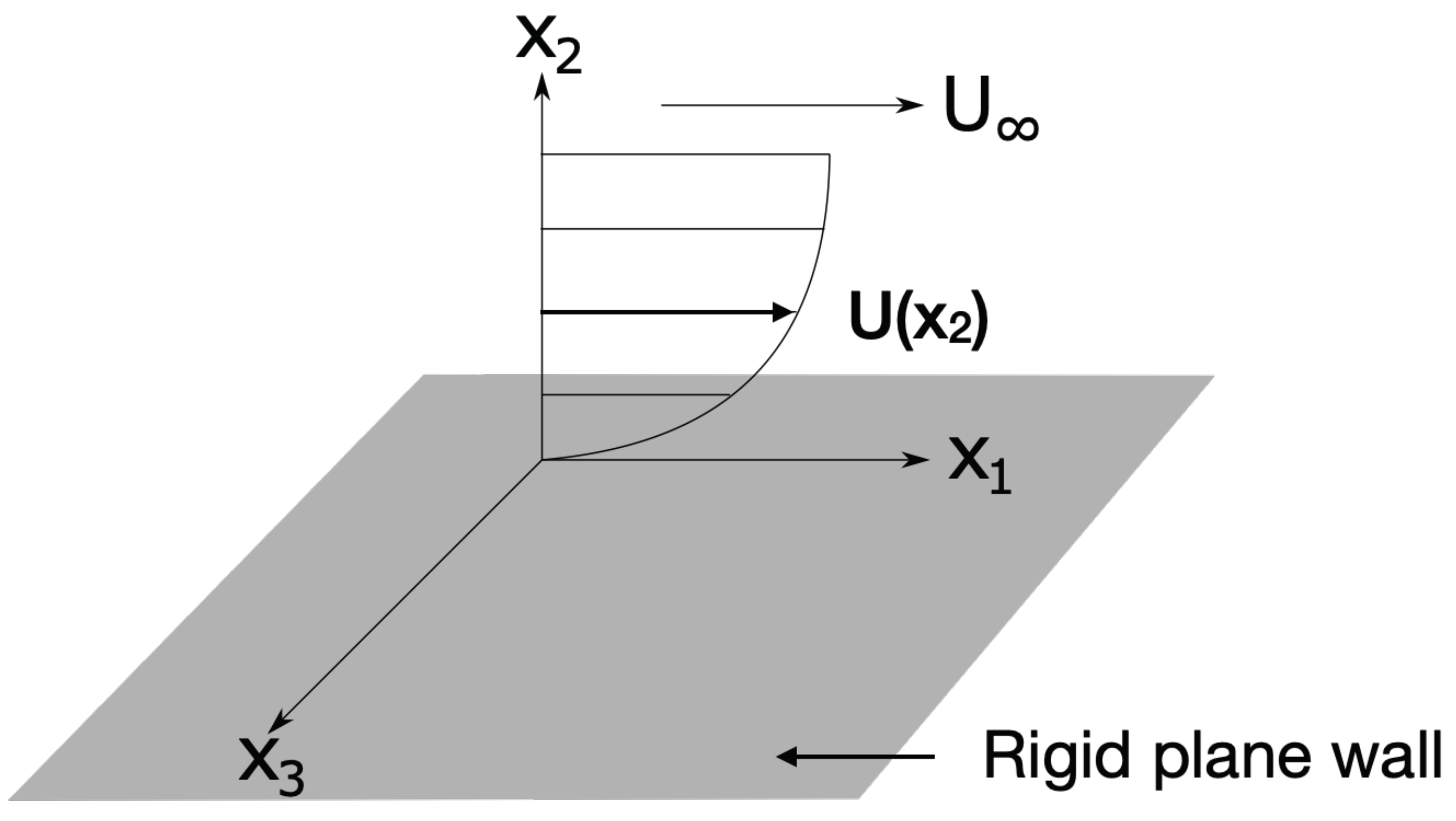
2. Theoretical Background

This section summarizes the demonstration of the expression of the unsteady pressure beneath a turbulent boundary layer in compressible flow conditions, laid out in the paper of Gerolymos et al. [7]. The compressible Navier–Stokes equations form the basis for this analytical model. The rationale is the same as in the incompressible problem developed in [15], but with the additional density variable. The first step consists in taking the divergence of the compressible momentum equations, which yields
2 x i t ( ρ u i ) + 2 x i x j ( ρ u i u j ) = 2 p + 2 τ i j x i x j + x i ( ρ f V i )
where f V i is the body acceleration. Subtracting from Equation (1), its Reynolds average yields the following form of the Poisson equation for the fluctuating pressure
2 p = 2 ρ ¯ u i x j u ¯ j x i + ρ ¯ u i x j u j x i u i x j u j x i ¯ Quasi - incompressible terms + ρ u i x j u j x i ρ u i x j u j x i ¯ + 2 ρ u i x j ρ u i x j ¯ u ¯ j x i + ρ u ¯ i x j u ¯ j x i + δ 2 τ i j x i x j + x i ( ρ f V i ρ f V i ¯ ) + ρ D D t 1 ρ D ρ D t + D V D t · ρ
with the following definitions:
D ( · ) D t ¯ = ( · ) t + u i ( · ) x i ¯ = ( · ) ¯ t + u i ¯ ( · ) ¯ x i + u i ( · ) x i ¯
and
D ( · ) D t = D ( · ) D t D ( · ) D t ¯ .
The subscripts i , j 1 , 2 , 3 , where the indices correspond to the coordinate system depicted in Figure 1. The first two source terms on the right-hand side of Equation (2) are known as quasi-incompressible terms and correspond respectively to the turbulence-mean shear and turbulence–turbulence interaction source terms of the incompressible Poisson equation, reproduced below for simplicity:
2 p = 2 ρ 0 u i x j u ¯ j x i Turbulence - mean shear ρ 0 u i x j u j x i u i x j u j x i ¯ Turbulence - turbulence .
The quasi-incompressible terms scale with the mean density component, ρ ¯ , whereas the remaining terms scale with the density fluctuations, ρ , as demonstrated by the dimensional analysis of ([7] Appendix A). Morkovin’s hypothesis [27] implies that for a low-Mach-number flow, the effects of compressibility on turbulence are due to the gradient of the mean density, the influence of the density fluctuations being a higher-order effect. This holds true in the limit of ρ / ρ ¯ 1 . Within this hypothesis, it is justified to retain only the quasi-incompressible terms in the solution to the compressible Poisson equation governing pressure fluctuations in a compressible boundary layer, thus obtaining an equation of the same structure as Equation (3). Furthermore, it is possible to discard in first approximation the turbulence–turbulence interaction quasi-incompressible term. This is a widely used assumption, following the work of Kraichnan [28] and Hodgson [29], who estimated that the turbulence–turbulence term makes up 4–6% of the mean-square unsteady pressure. In particular, the analytical solution of Equation (3) with the turbulence–turbulence component alone on the right-hand side, developed by Hodgson, was re-derived and generalized in [15] and applied to the CD airfoil configuration in the incompressible flow regime. It was thus confirmed that the turbulence–turbulence component is negligible with respect to the turbulence–mean shear over the low-to-middle frequency range. Therefore, the quasi-incompressible Poisson equation is
2 p = 2 ρ ¯ u i x j u ¯ j x i .
The mean density, ρ ¯ , at the right-hand side of Equation (4), varies in space, which is the mean difference between this equation and the incompressible one. Performing the Fourier transform of Equation (4) in space along the wall directions ( x 1 , x 3 ) in time and applying the classical boundary-layer approximation, for which the mean flow speed is aligned with the x 1 axis, and the only non-vanishing mean velocity gradient is that of the stream-wise velocity u ¯ 1 in the wall-normal direction x 2 (as depicted in Figure 1), we obtain the following inhomogeneous Helmholtz equation:
p ^ ( ω , k , x 2 ) x 2 2 k 2 p ^ ( ω , k , x 2 ) = 2 ρ ¯ ( x 2 ) i k 1 u ¯ 1 ( x 2 ) x 2 u ^ 2 ( ω , k , x 2 ) ,
where k = ( k 1 , k 3 ) . The boundary-layer model used in the derivation of the previous equation is valid for actual boundary layers as long as their thickness is much smaller than the local radius of curvature of the surface (i.e., quasi-parallel flow). Assuming that the unsteady pressure vanishes at an infinite distance from the wall, that is
lim x 2 p = 0 ,
and adopting the rigid-wall model whereby
p x 2 x 2 = 0 = 0
we can write the well-known Green’s function solution (see for instance [7]) to the differential equation above as
p ^ ( ω , k , x 2 = 0 ) = 2 i k 1 k 0 + ρ ¯ ( X 2 ) u ^ ( ω , k , X 2 ) u ¯ 1 ( X 2 ) x 2 e k X 2 d X 2 .
Multiplying Equation (6) by its complex conjugate and taking the ensemble average of the result yields the general expression of the wall-pressure power spectral density:
Φ p p T M ( ω , k 1 , k 3 ) = 4 k 1 2 k 2 ω k 0 ρ ¯ ( X 2 ) ρ ¯ ( X 2 ) e ( X 2 + X 2 ) k U 1 ( X 2 ) x 2 U 1 ( X 2 ) x 2 × u ^ ( ω , k , X 2 ) u ^ ( ω , k , X 2 ) d X 2 d X 2 d k d ω .
The superscript T M reminds one that this solution only takes into account the turbulence–mean shear interaction source term.
Due to the statistical orthogonality of the turbulence wave-vectors [30], the ensemble average of the product of vertical velocity fluctuations can be written as
u ^ ( ω , k , X 2 ) u ^ * ( ω , k , X 2 ) = φ 22 ( ω , k , X 2 , X 2 ) δ ( k k ) δ ( ω ω )
and then the wall-pressure PSD becomes
Φ p p T M ( ω , k 1 , k 3 ) = 4 k 1 2 k 2 0 ρ ¯ ( X 2 ) ρ ¯ ( X 2 ) e ( X 2 + X 2 ) k U 1 ( X 2 ) x 2 U 1 ( X 2 ) x 2 × φ 22 ( ω , k , X 2 , X 2 ) d X 2 d X 2 .
According to Equation (8), the frequency-wavenumber PSD of the wall-pressure flucutation is directly proportional to the normal-to-wall variation of mean density, mean shear and to the cross-spectral density of vertical velocity fluctuations, φ 22 . The first two quantities can be computed by means of a steady-state compressible flow simulation. The latter, however, needs to be modeled for practical applications. The turbulent cross-spectral density can be expressed as the product of a wavenumber cross-spectrum and a moving-axis spectrum, where the latter expresses the frequency dependency:
φ 22 ( ω , k , X 2 , X 2 ) = φ 22 ( k , X 2 , X 2 ) Φ m ( ω U c k 1 ) .
The wavenumber term can be represented with various analytical formulations according to different theories. The Generalized von Kármán Spectrum, as defined in [31,32], is a useful formulation of the wavenumber term because, depending on the value of one parameter, it reduces to either the classical von Kármán, the Liepmann or the Rapid Distortion Theory turbulence spectrum. Assuming homogeneous and isotropic turbulence, the Generalized von Kármán spectrum has the following expression:
φ 22 k , x 2 , x 2 = u 2 2 ¯ ( x 2 ) u 2 2 ¯ ( x 2 ) l 2 k ˜ 2 ζ ν + 2 Γ ( ν ) π 2 ν + 1 1 + k ˜ 2 ν + 2 K ν + 2 ( ζ )
with the parameter
ζ = x 2 x 2 l 1 + k ˜ 2 .
and the characteristic length scale
l = Γ ( ν ) π Γ ( ν + 1 / 2 ) Λ ,
where Λ is the turbulent longitudinal integral length scale. If ν = 1 / 3 , Equation (10) corresponds to the model of von Kármán [33], if ν = 1 / 2 to Liepmann’s model [34] and if ν = 7 / 6 to the rapid distortion theory (RDT) [35]. In order to close the model, in earlier works [15,19] Taylor’s hypothesis of frozen turbulence convection has been applied, whereby the moving axis spectrum is a Dirac delta function centered at the convective frequency ω = U c k 1 :
Φ m D ( ω U c k 1 ) = δ ( ω U c k 1 ) ,
where U c is the convective speed of velocity fluctuations. In this case, the wall-pressure spectral density at a given frequency ω is uniquely determined by turbulent fluctuations at the streamwise wavenumber K 1 = ω / U c . However, the Dirac formulation of the moving-axis spectrum does not ensure the decay of the wall-pressure coherence function in the streamwise direction, x 1 . Furthermore, it can be interesting to keep the functional dependency of the wall-pressure PSD expressed in Equation (8) on both ω and k 1 . To solve both problems, the formulation of the moving-axis spectrum given in the TNO-Blake model (see [8]) as a Gaussian function centered around the convective frequency, can be used:
Φ m G ( ω U c k 1 ) = 1 α 2 2 π exp ( ω U c k 1 ) 2 2 α 2 2
with
α 2 = c 6 U c Λ 2 .
In the original TNO model, the coefficient c 6 is assumed constant and equal to 0.05.
Finally, this model needs to account for the anisotropy of turbulent structures, defined as the ratio of longitudinal-to-transverse integral length scales, α . Following Schlinker and Amiet [36], the anisotropic turbulence vertical cross-spectral density, φ 22 N I , is defined with respect to the isotropic formulation of Equation (10), φ 22 I , as
φ 22 N I ( k 1 , x 2 , x 2 , k 3 ) = α φ 22 I ( α k 1 , x 2 , x 2 , k 3 ) .
In principle, the anisotropic coefficient α varies in the normal-to-wall direction; however, it has been shown in [15,19] that a constant representative value of α may suffice for the prediction of the wall-pressure spectral density in the frequency range of interest.

3. Study of the Controlled-Diffusion Airfoil Test Case

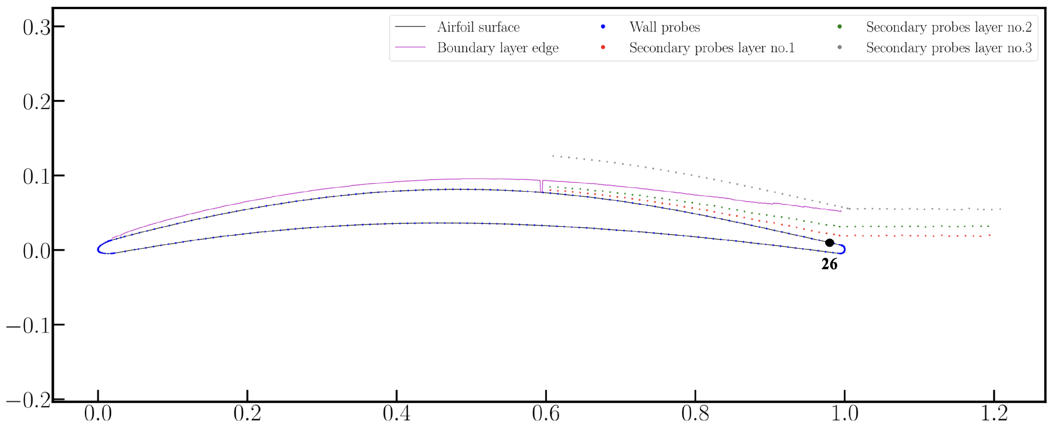
3.1. Large Eddy Simulation of the Flow around a Controlled-Diffusion Airfoil

This section presents the post-processing of the LES of the flow around the CD airfoil, which was in turn performed at ISAE-Supaéro [20,21] in the framework of the European project SCONE. The wall-resolved LES (WRLES) has been performed by means of the massively parallel compressible solver CharLESX, which offers a low dissipation cell-centered finite-volume scheme. The numerical solution method is second-order accurate in space and third-order accurate in time, using a low-storage Runge–Kutta–Wray scheme for explicit time advancement. The sub-grid turbulent scales (SGS) are represented by Vreman’s model. The unstructured computational grid has an O-grid topology and is made up of 225.5 M cells. The computational domain extends 20 c , where c is the airfoil chord, in both the streamwise and normal-to-wall directions and 0.1 c in the transverse direction. The dimensionless wall distance, y + , on the CD airfoil surface is below 1.12 . The normalized time step is 2.68 × 10 5 . The mesh resolution quality has been verified by means of Pope’s criterion [37], which measures the ratio of resolved to total (i.e., sum of resolved and SGS) turbulent kinetic energy. This ratio is found to be at least 0.94 for all the WRLES simulations performed in the SCONE project, meaning that the resolution level is close to that of a DNS mesh.

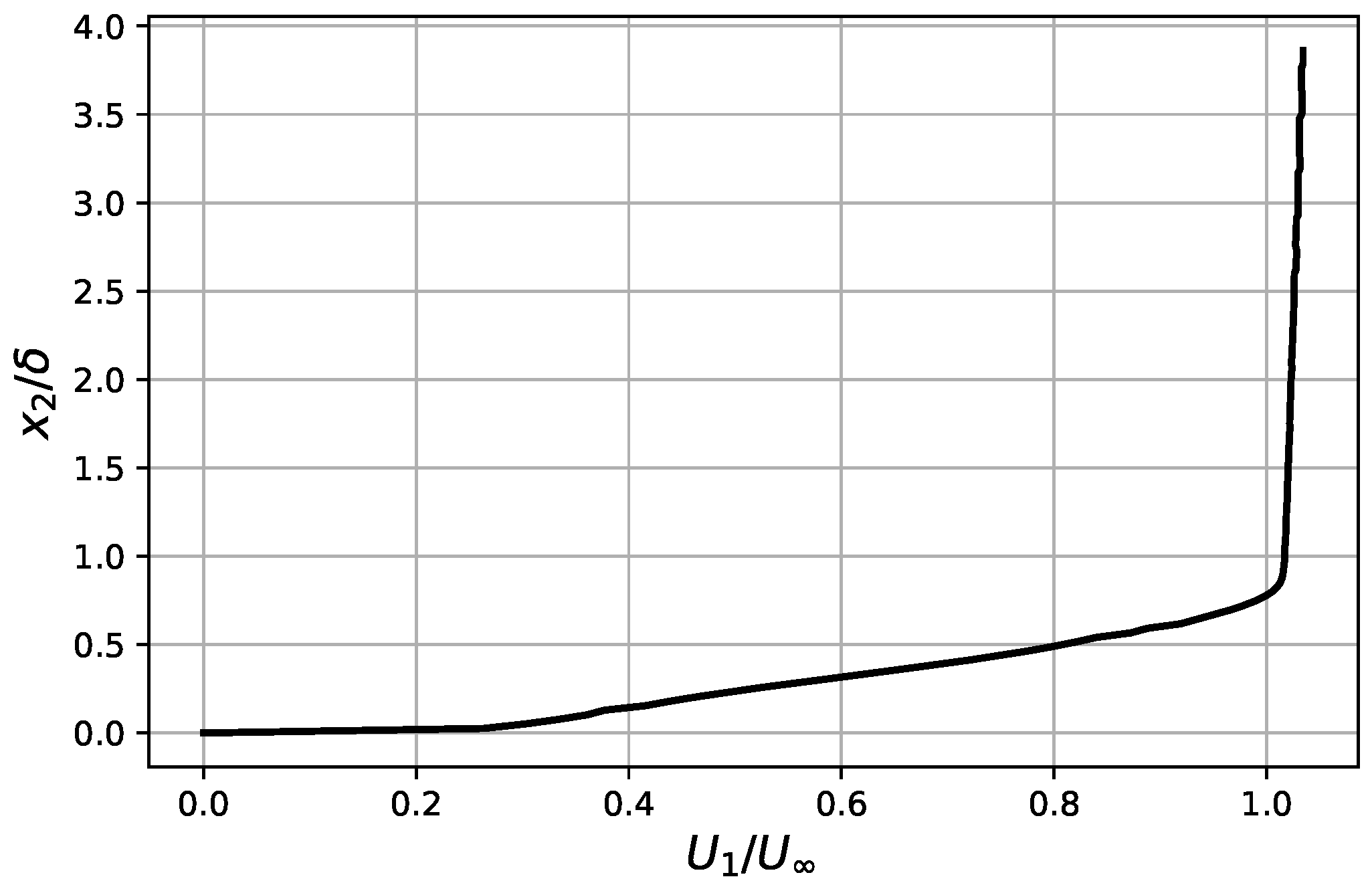
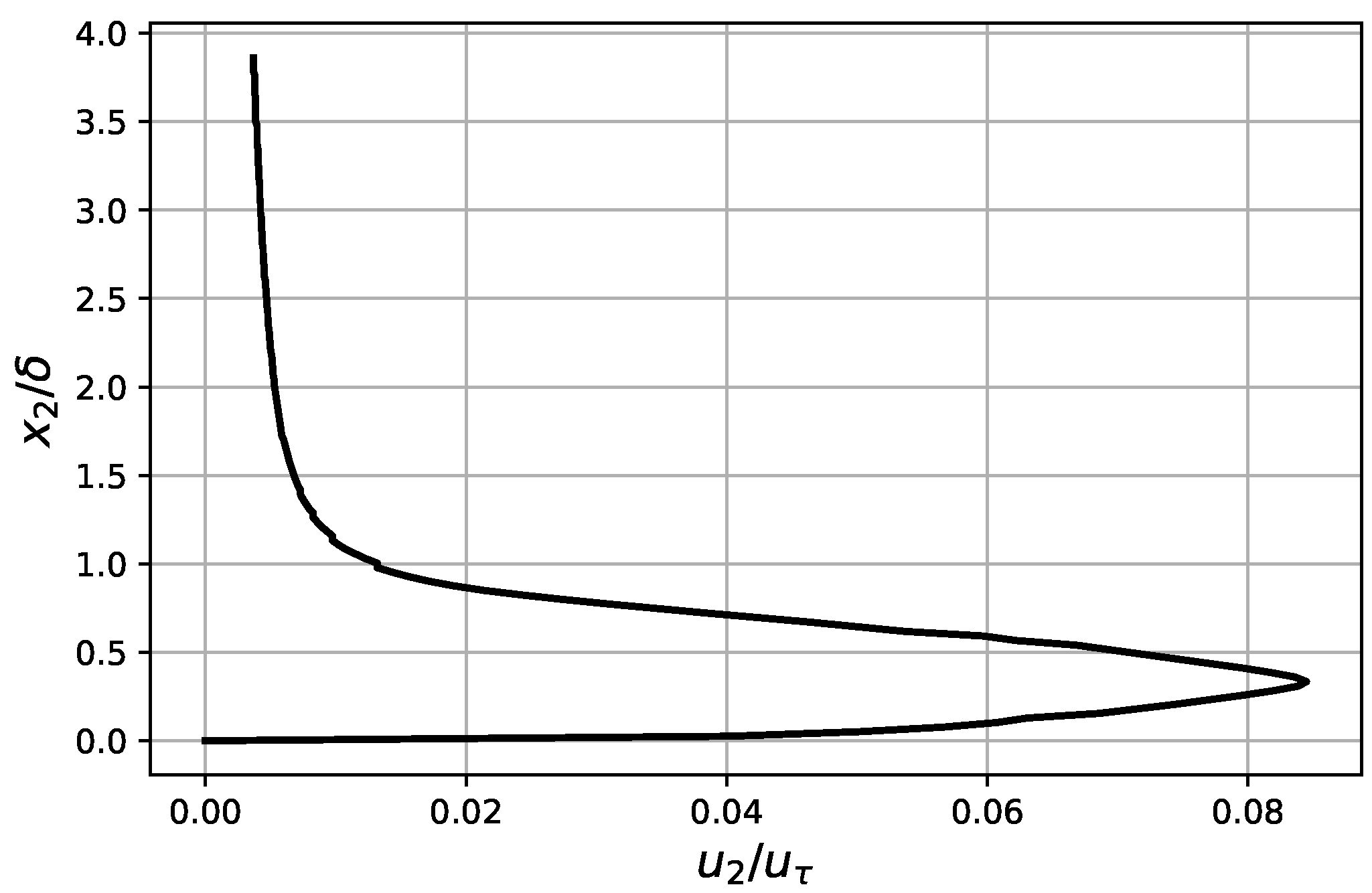
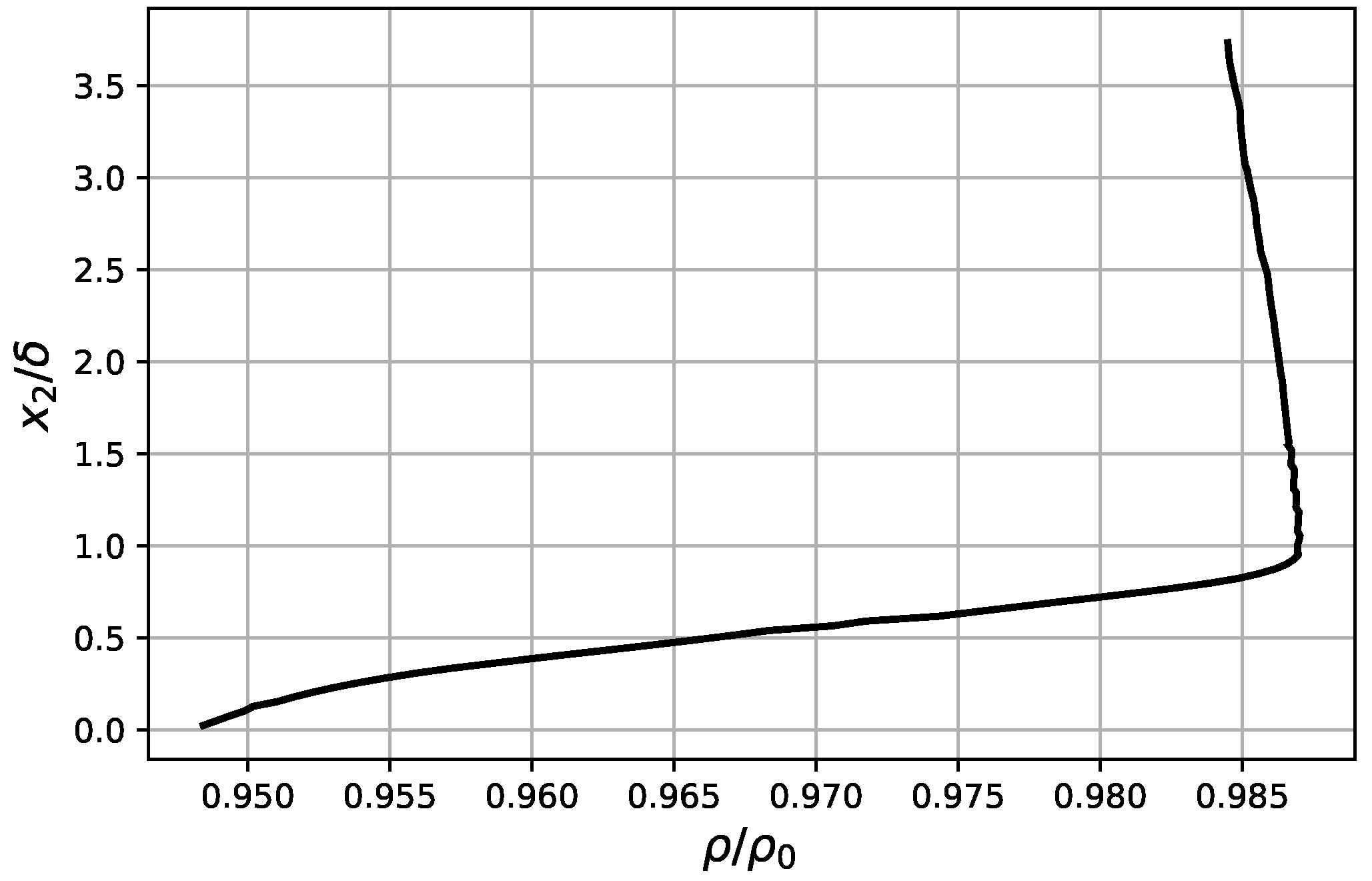
3.2. Boundary Layer Profiles Close to the Trailing Edge of the Airfoil

As observed in the previous section, the boundary layer profiles and the statistical properties of the turbulent flow are the necessary input data to the wall-pressure PSD analytical model. These quantities are extracted from the LES simulation close to the trailing edge of the CD airfoil, at 2 % of chord upstream of the trailing edge, corresponding to the position of pressure sensor number 26 in the experimental setup (see Figure 2). It is interesting to predict the wall-pressure statistics as close as possible to the edge of the profile, because they determine the amplitude and frequency distribution of the corresponding radiated noise (see [26] for an investigation of this dependence). Figure 3 and Figure 4 show the mean stream-wise and the RMS normal-to-wall velocities, respectively. The mean density, ρ ¯ , has a moderate 4 % variation from the wall to the edge of the boundary layer, as can be observed in Figure 5.

3.3. Turbulence Statistics

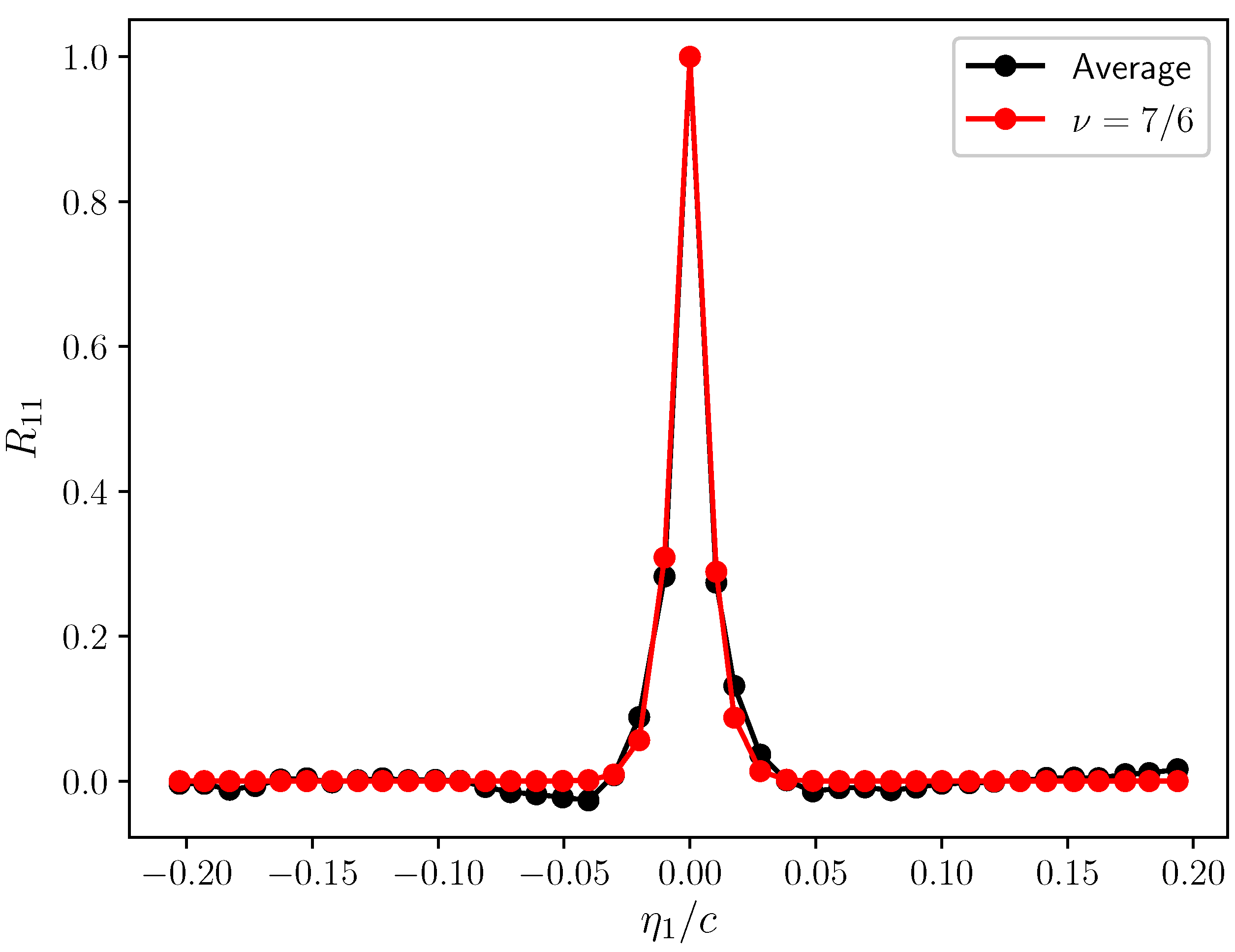
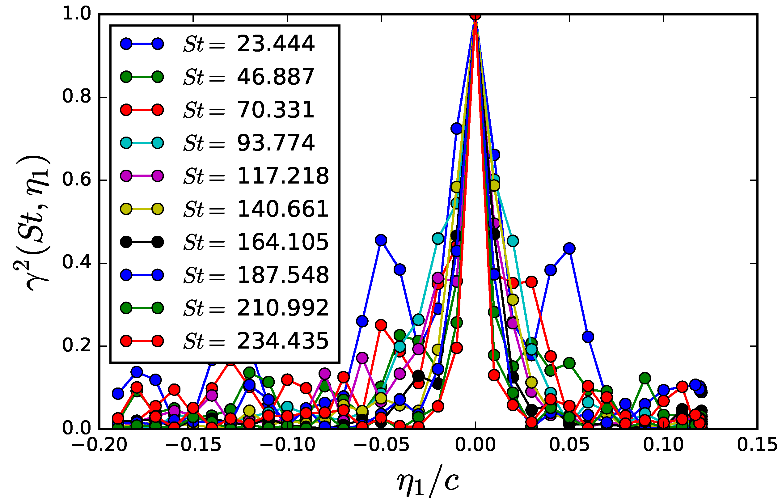
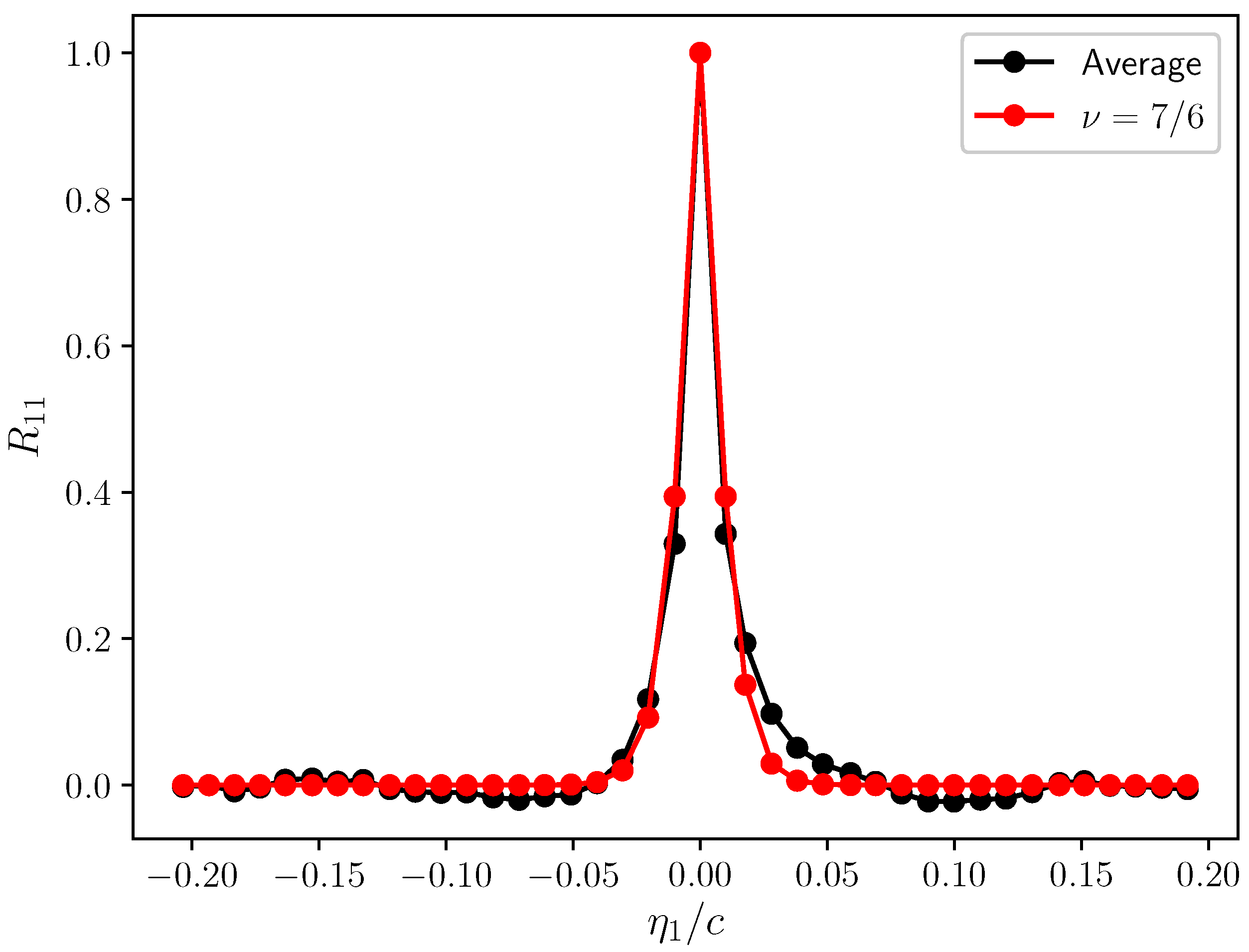
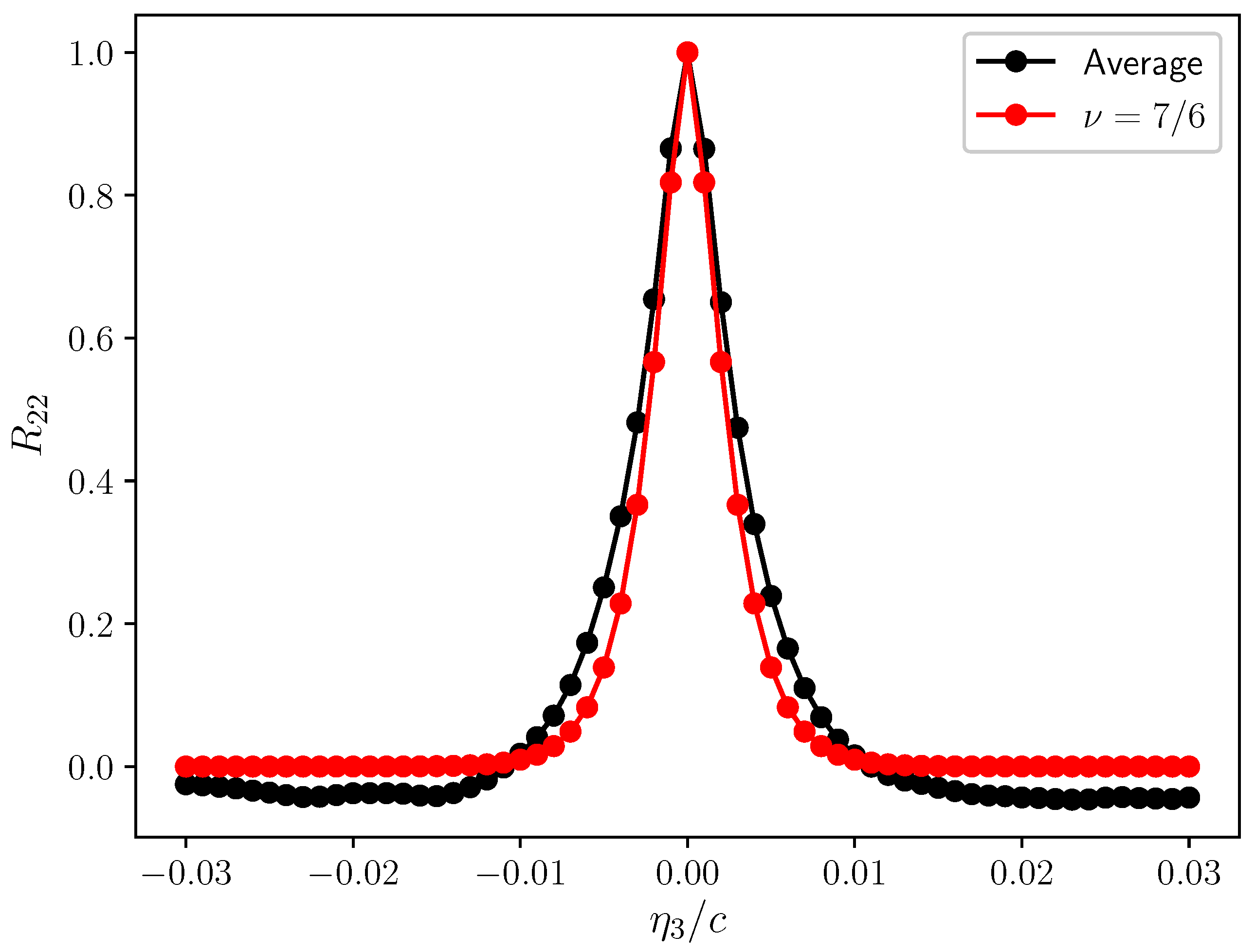
3.3.1. Streamwise and Transverse Velocity Correlation Coefficient

Unsteady velocity time series have been extracted from the LES only on three mesh layers parallel to the airfoil surface, depicted in Figure 2. Furthermore, as can be observed in Figure 2, the upper mesh layer lays outside the boundary layer; therefore, the study of turbulence statistics will be focused on the two inner mesh layers.
The first statistical property of the turbulent field that is calculated is the correlation coefficient. Considering a homogeneous turbulence field, this quantity is defined as
R i j ( η 1 , η 2 , η 3 ) = u i ( x 1 , x 2 , x 3 ) · u j ( x 1 + η 1 , x 2 + η 2 , x 3 + η 3 ) σ 2
where σ 2 is the variance of turbulent velocity fluctuations. In the framework of the Generalized von Kármán theory, this correlation coefficient is expressed analytically as
R i j ( η 1 , η 2 , η 3 ) = 1 2 ν 1 Γ ( ν ) η l ν η i η j η 2 K ν η l + δ i j 1 η i η j η 2 ( ν + 1 ) K ν η l 1 2 η l K ν + 1 η l
where η = η 1 2 + η 2 2 + η 3 2 and K ν is the modified Bessel function of the second kind of order ν . The correlation coefficient R 22 is of particular interest because it is related to the vertical velocity cross-spectral density, φ 22 , by the double spatial Fourier transform:
φ 22 ( k 1 , η 2 , k 3 ) = σ 2 4 π 2 + R 22 ( η 1 , η 2 , η 3 ) cos ( η 1 k 1 ) cos ( η 3 k 3 ) d η 1 d η 3 .
Therefore, the choice of the analytical formulation of φ 22 could be validated directly by calculating the vertical velocity correlation coefficient, R 22 ( η 2 ) , from the CFD data and comparing it with Equation (17) (see [15], Figure 12 for an example of this comparison). However, as the unsteady velocity time series has been recorded only on two mesh layers inside the turbulent boundary layer, there are not enough points for comparing the analytical and the directly computed correlation. For this reason, the choice of the value of ν in Equations (10) and (17) will be based on the calculation of the streamwise ( R 11 ( η 1 ) ) and transverse ( R 33 ( η 3 ) ) velocity correlation coefficients, under the assumption that the vertical correlation behaves in the same way.
Figure 6 and Figure 7 depict the streamwise velocity correlation coefficient calculated on mesh layers 1 and 2, respectively. The following Figure 8 and Figure 9 depict the transverse velocity correlation coefficient on the same mesh layers parallel to the airfoil surface. It can be observed in these plots that the Rapid Distortion Theory (RDT) [35] convincingly describes both the longitudinal and the transverse correlation coefficients inside the boundary layer. This is consistent with the finding of Magnaudet (see [38]) that the RDT is the leading-order approximation describing the short-term and long-term evolution of turbulent boundary layers in the limit of the large Reynolds number. Furthermore, the fundamental assumption of the RDT is that the turbulence–turbulence interaction is negligible with respect to the turbulence–mean shear interaction (see also [30]), which is exactly the same hypothesis that has been made in the derivation of Equation (8). Therefore, the use of the RDT to model the vertical velocity cross-spectral density, φ 22 , is arguably the most consistent choice with the fundamental assumption of the model that has been laid out in Section 2.

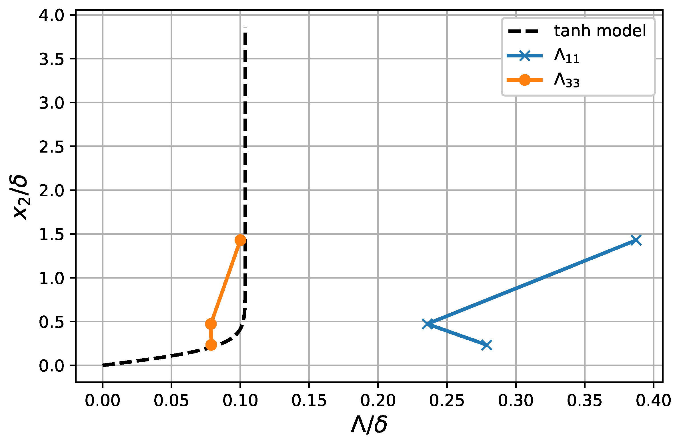
3.3.2. Integral Length Scale and Anisotropy Coefficient

The longitudinal and transverse integral length scales are available only at three locations above the wall, as shown in Figure 10. However, a continuous function of Λ versus the distance from the wall, x 2 , is necessary in order to calculate the integral in Equation (8). For this reason, a working hypothesis is made to represent the transverse length scale with a physically-consistent model based on the hyperbolic tangent function, following the empirical considerations of Parchen [39] (see also [8] and [15], Equation (2.38)). The model is here re-scaled in order to match the transverse length scale as closely as possible. Considering the available values of the ratio between the longitudinal and transverse scales, the value of α = 3.5 will be used in the prediction of wall-pressure statistics.

4. Direct Computation and Empirical Modeling of Wall-Pressure Statistics

The time series of wall-pressure fluctuations, p , recorded on the airfoil-surface grid, can be used to compute directly various statistical properties. Figure 11 shows the coherence function of p for various values of the Strouhal number, S t , taking the reference point at 12 % of the chord upstream of the trailing-edge and shifting the second point in the stream-wise direction. This reference point has been taken more upstream in order to be able to assess the coherence function both upstream and downstream. The plot shows a faster decay of the correlation function for a higher S t . Figure 12 represents the phase of the cross spectrum of wall-pressure fluctuations versus the stream-wise coordinate. Assuming that the phase is linear, its slope is directly proportional to the convective speed of wall-pressure fluctuations, U c , for a given frequency, ω . Following the method described in [40], the linear function ω η 1 / U c is fitted to the phase in order to estimate the value of U c . This value is needed for the prediction of the wall-pressure PSD because it is part of the definition of the moving-axis spectrum. Furthermore, it is needed in the analytical modeling of the trailing-edge noise, according to Amiet’s model, as mentioned in the introduction. As can be observed in the plots, the linear fit is not a trivial operation, neither at low nor at high frequency, due to the scarcity of the sample points.
The variation of U c with the frequency is shown is Figure 13. Interestingly, Smol’yakov’s empirical model [41] predicts a peak at the same value of the normalized abscissa ω δ 1 / U , where δ 1 is the boundary layer displacement thickness. However, the amplitude of the peak is subject to the uncertainty of the linear interpolation. On the contrary, for normalized frequencies above 0.6 , the ratio stabilizes around U c / U = 0.5 . It is therefore safer to use this constant value of U c in the predictions presented in the next section.
Finally, Figure 14 presents the transverse coherence function γ 2 ( ω , η 3 ) , as a function of the chord-based Strouhal number, for various separations η 3 in the span-wise direction. As expected, the coherence decreases with a separation at any frequency. It exhibits a maximum for some relatively low frequencies and a drop at very low frequencies. Yet, this drop is hard to estimate accurately because of the suspected lack of convergence in the numerical simulations. A log-normal distribution of the coherence has often been found in previous low-speed experiments, as reported for instance in [42]. Attempting such a fit on the present data is less convincing at high frequencies, as illustrated in Figure 15. The theoretical expression plotted as the blue mesh reads
γ 2 ( f , η 3 ) = A σ 2 π S t e ( log 10 ( S t ) log 10 ( S t 0 ) ) 2 / ( 2 σ 2 ) ,
with S t 0 = 1.5 0.06 η 3 , A = 20.5 e 0.19 η 3 , σ = 0.53 0.02 η 3 , the separation being in mm. In particular, the high-frequency behavior deviates from the trend at larger separations. It is also worth noting that the decay with η 3 at a given frequency is not exactly exponential, according to both the fit and the extracted data. Further investigation is needed to elucidate whether the coherence includes specific effects of compressibility.

5. Prediction of Wall-Pressure Statistics with the Analytical Model Based on the Poisson Equation

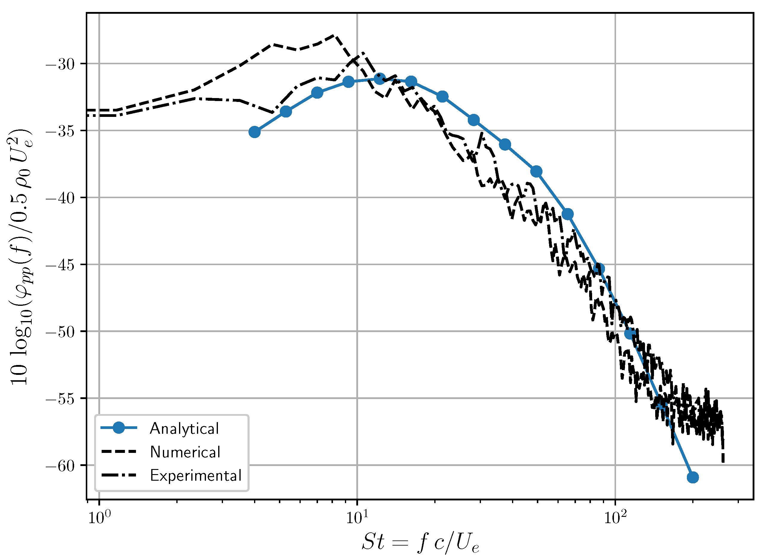
5.1. Single-Point Statistics

As a first example of the application of the model based on the Poisson equation, the single-point PSD of wall-pressure fluctuations is predicted by means of Equation (8). In this case, the wavenumber component of the cross-PSD of vertical velocity fluctuations is modeled by means of the RDT. Taylor’s hypothesis completes the turbulence model and allows us to reduce the computational time by eliminating one dimension of integration. The same strategy has been followed successfully in [15,19]. The input data are the boundary layer profiles presented in Section 3.2 and the integral length scale presented in Figure 10, along with the values of α and U c determined empirically from the LES results. The integration of Equation (8) is performed by means of a recursive stratified sampling Monte-Carlo method (see [15,43] for further details) implemented in the Python scikit-monaco library [44]. The wall-pressure PSD prediction is shown in Figure 16, where it is compared with a measured spectrum, obtained by NLR in the framework of the CRORTET project [45], and with the spectrum calculated directly from the LES. The measured and LES spectra are taken at 2 % of the chord upstream of the trailing edge, consistently with the extraction of the boundary layer profiles. The convincing overall agreement confirms the relevance of the model. In particular, the high-frequency roll-off is very well captured.

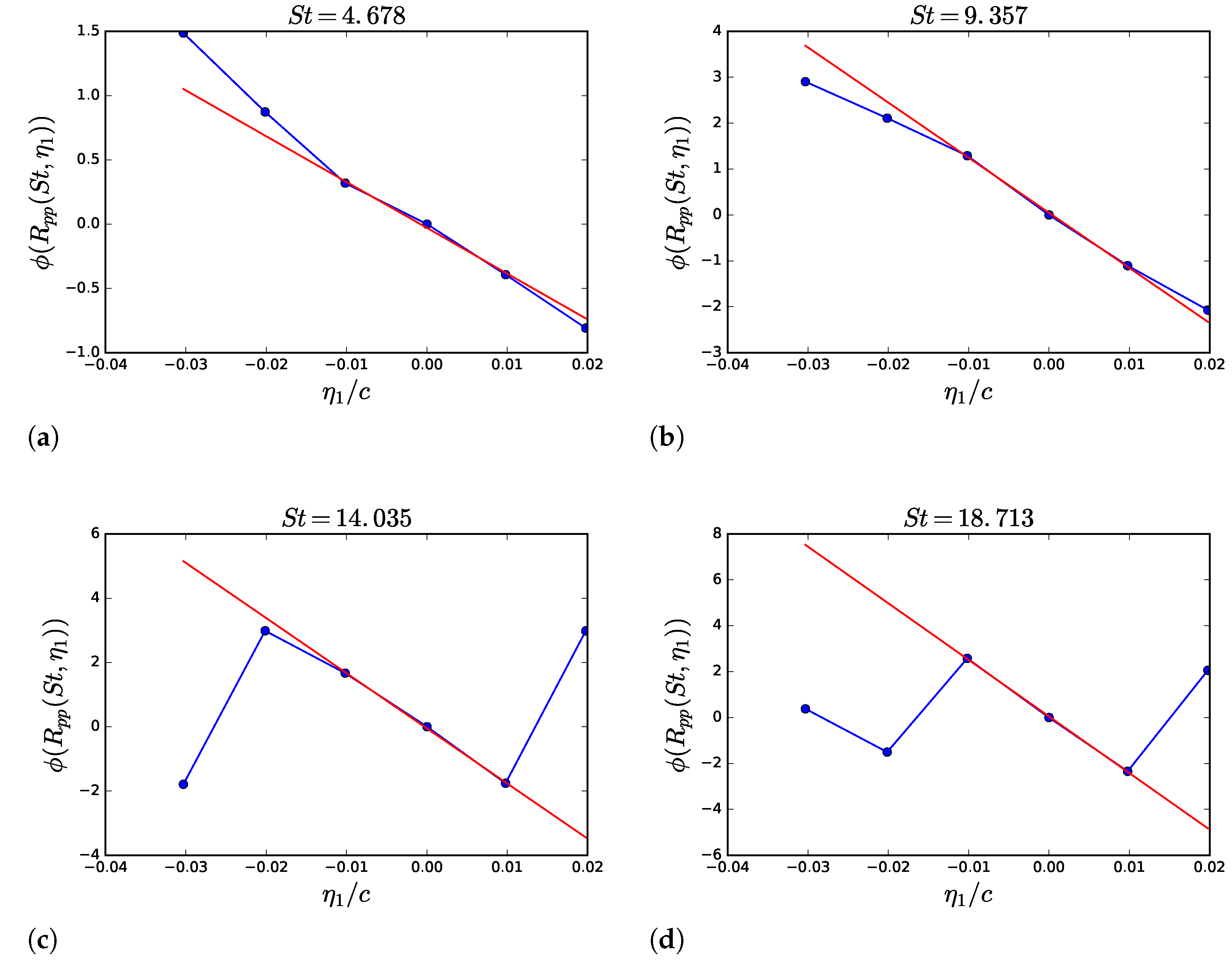
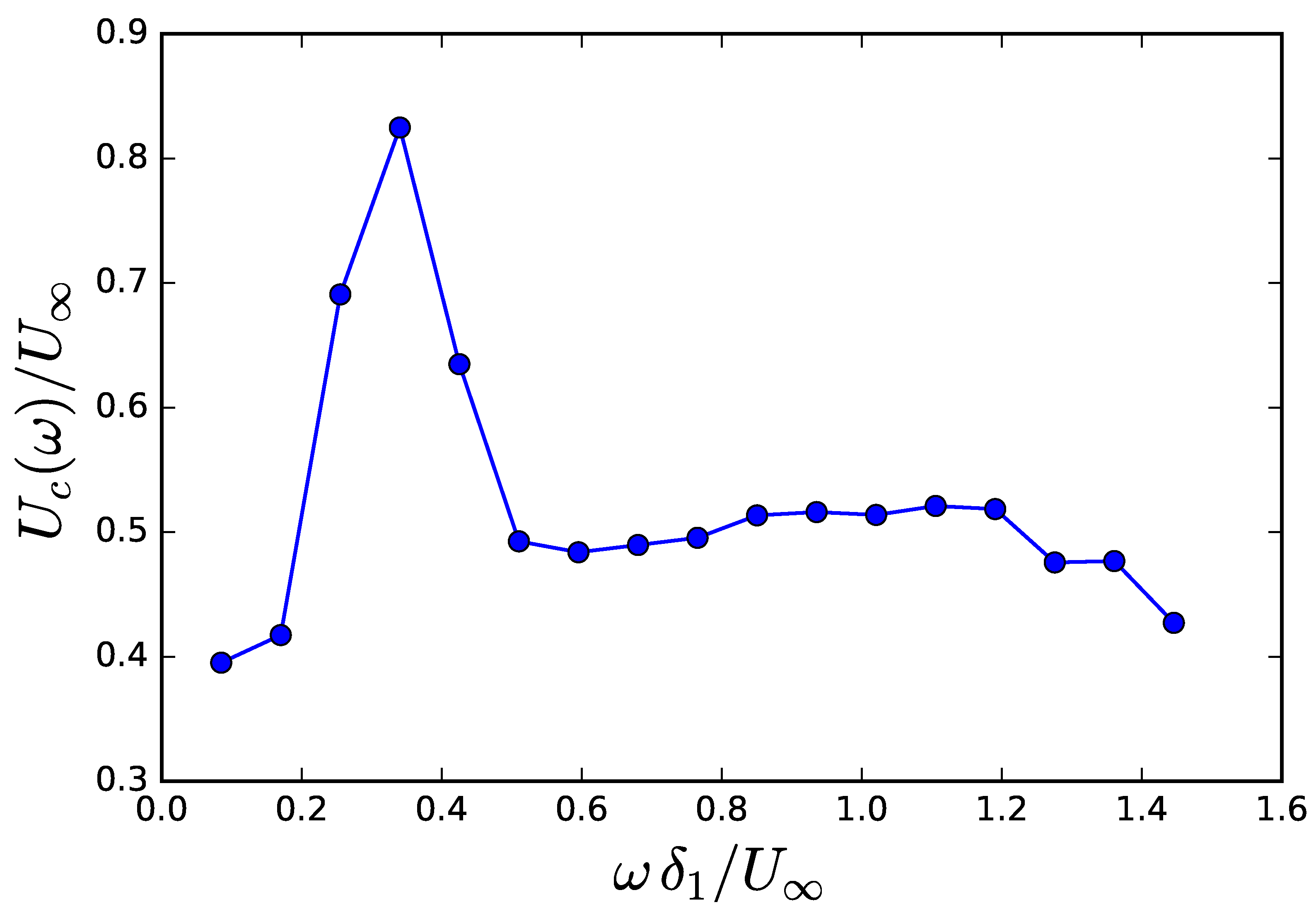
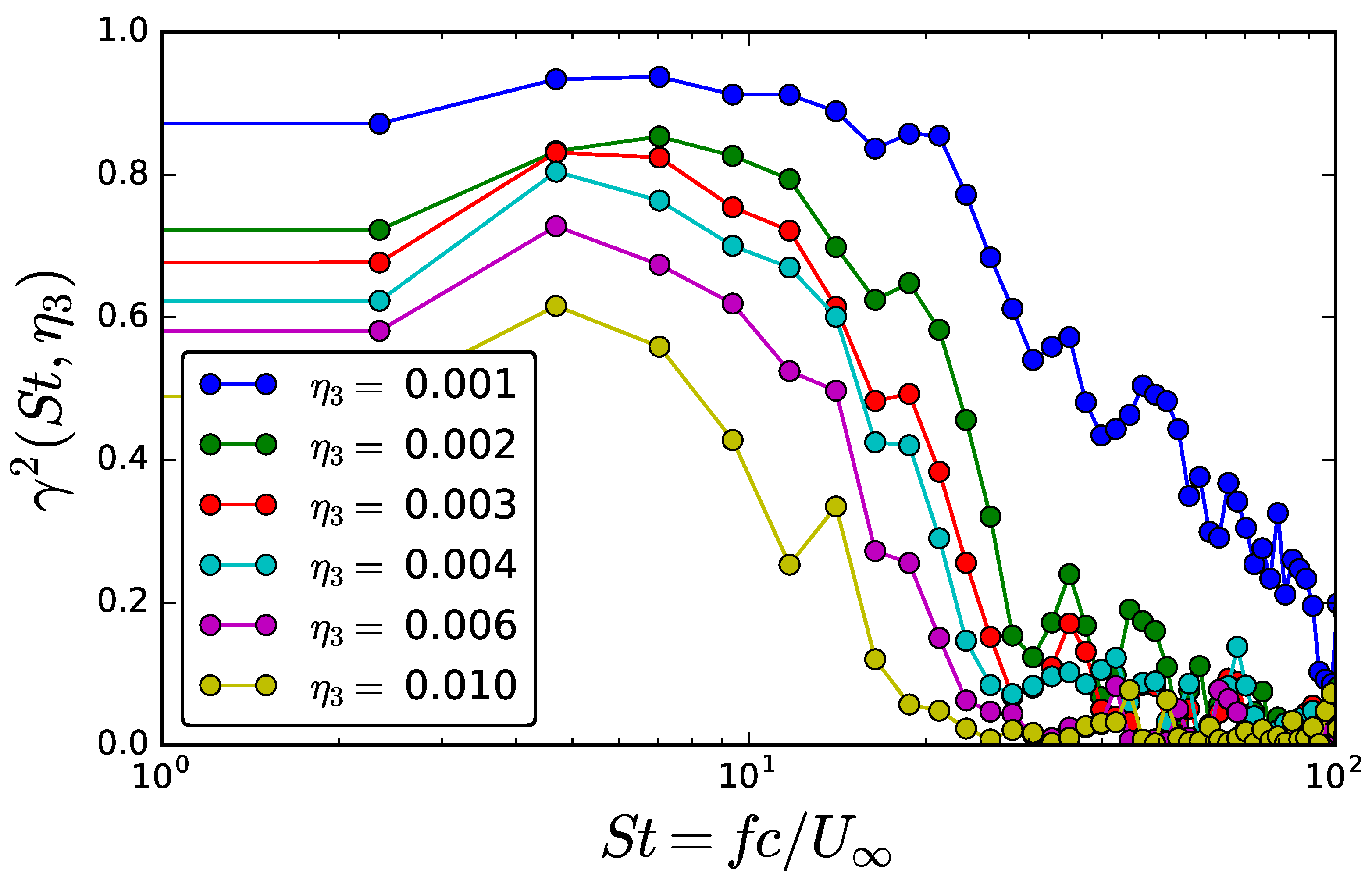
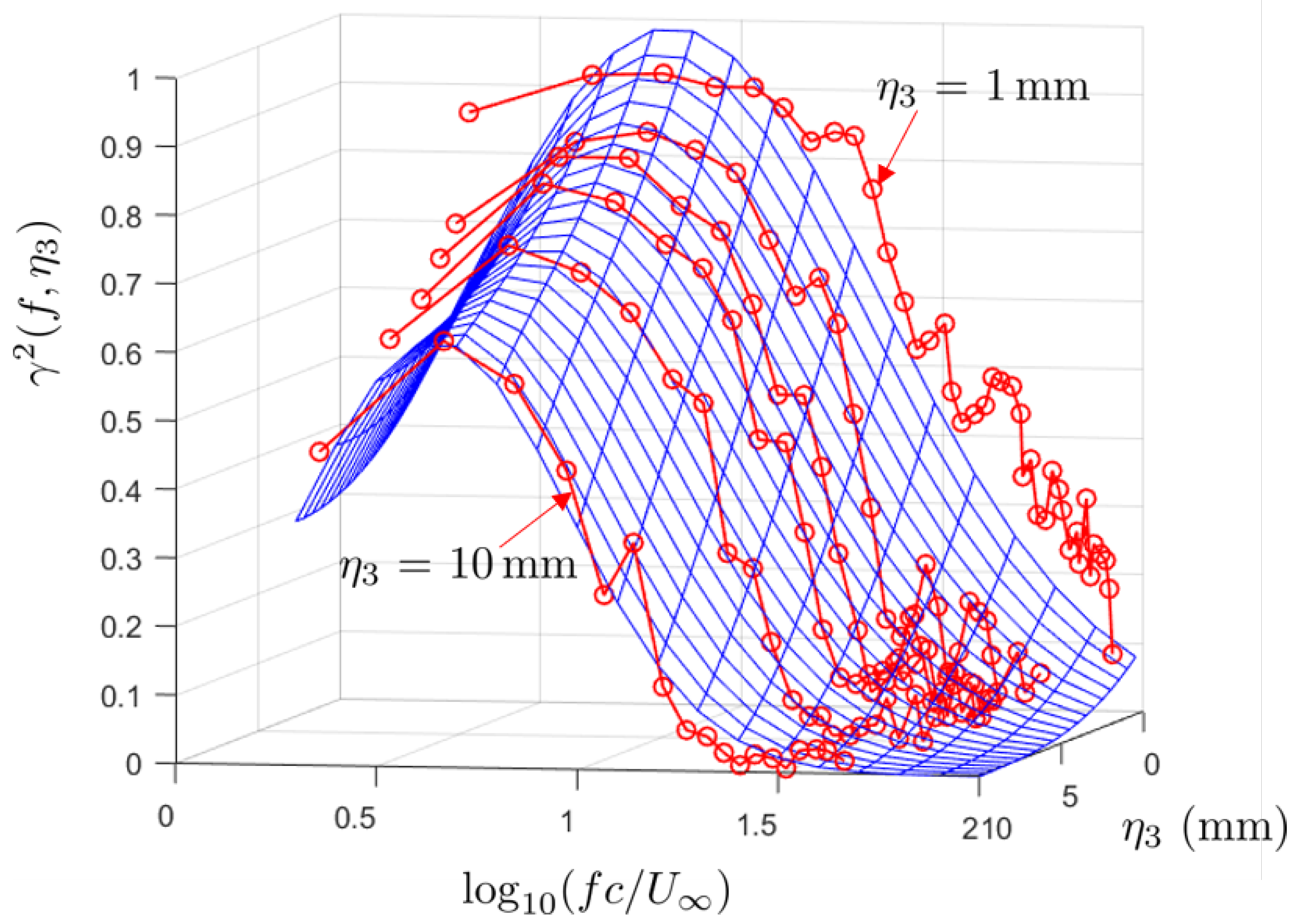
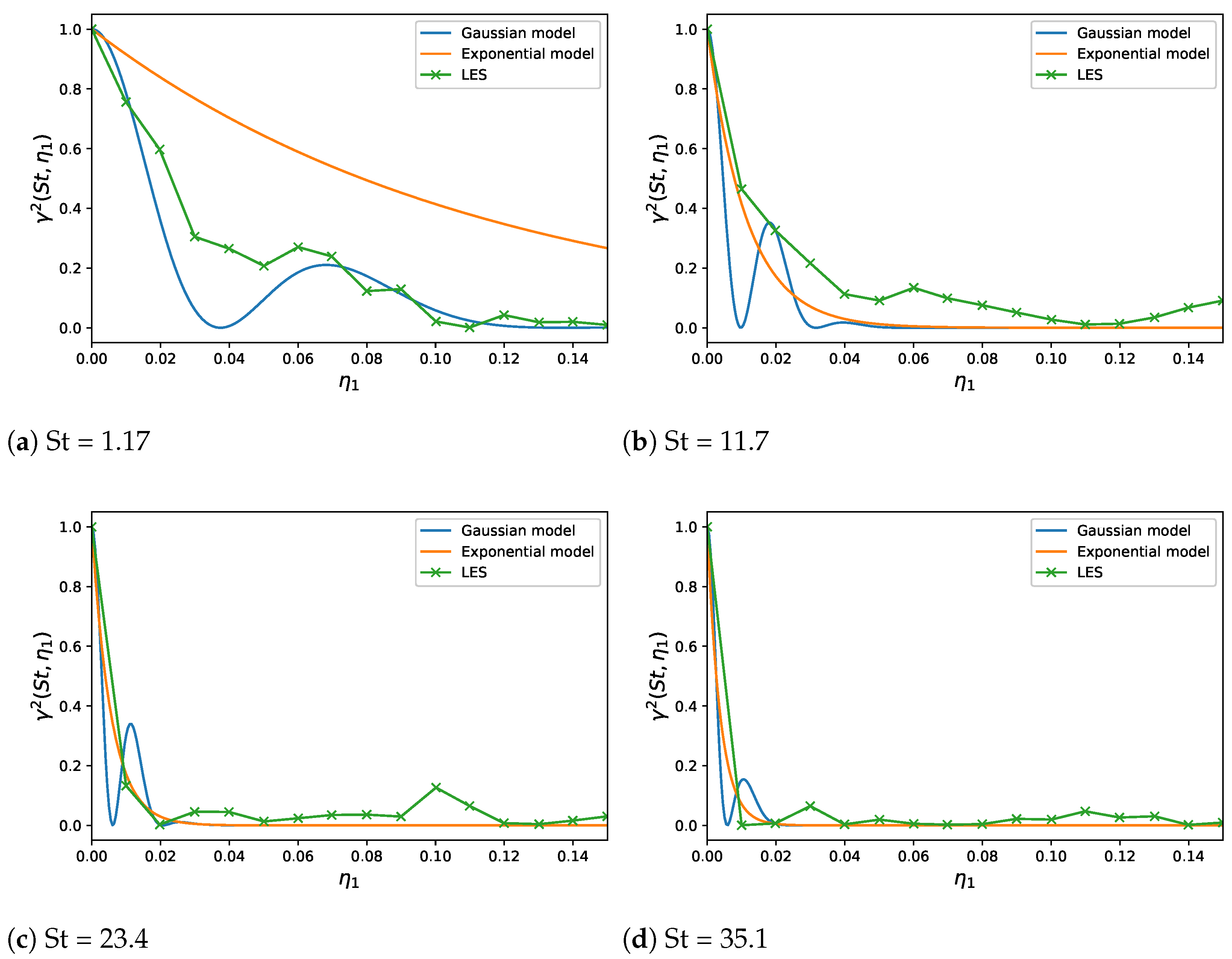
5.2. Multi-Point Statistics

Equation (8) can also be used to model the wall-pressure coherence function. Assuming homogeneity of the wall-pressure fluctuations on the wall surface, the corresponding wall-pressure coherence function can be formulated as the (normalized) inverse spatial Fourier transform of the wall-pressure PSD:
γ 2 ( ω , η j ) = 0 Φ p p ( ω , k 1 , k 3 ) cos ( k j η j ) d k 1 d k 3 2 0 Φ p p ( ω , k 1 , k 3 ) d k 1 d k 3 2
where j 1 , 3 . The substitution of the frequency-wavenumber wall-pressure spectrum given by Equation (8) in Equation (19) for the calculation of the coherence implies the use of the Gaussian moving-axis spectrum formulation of Equation (14) in order to separate the frequency and wavenumber variables.
The Dirac formulation of the moving-axis spectrum following the hypothesis of frozen turbulence, on the contrary, is not applicable to the calculation of the coherence function because it does not ensure the decay of the coherence with distance. For this reason, Blake [46] proposes the following empirical correction to the Dirac formulation, which introduces an exponential decay in the longitudinal direction:
Φ m ( ω U c k 1 , η 1 ) = δ ( ω U c k 1 ) e γ B | ω η 1 / U c |
where γ B is an empirical parameter ranging between 0.2 and 0.3 . Substituting Equation (20) in Equation (8), the longitudinal coherence function is simply
γ 2 ( ω , η 1 ) = e 2 γ B | ω η 1 / U c | .
Figure 17 compares the longitudinal wall-pressure coherence extracted from the LES simulation and predicted by means of the numerical integration of Equation (19), using the Gaussian formulation of the moving-axis spectrum given in Equation (14). The empirical exponential decay of Equation (21) is also plotted in Figure 17, using the value γ B = 0.3 . The reference point is the same for which the single-point statistics have been computed; the η 1 coordinate is directed upstream. The Gaussian formulation of the moving-axis spectrum better captures the LES-predicted trend at the lowest Strouhal number, whereas for increasing frequency the difference between the two formulations decreases. Interestingly, the Gaussian formulation predicts a second smaller local maximum of the longitudinal coherence function, which is difficult to see in the LES data, especially at high frequencies, due to the relative coarseness of the surface mesh.
Figure 18 shows the transverse correlation as a function of the Stouhal number for two values of the transverse separation, since the LES time series of pressure fluctuations have been recorded for a smaller number of points in the η 3 direction. The LES transverse coherence is compared with the model based on the Gaussian moving axis spectrum alone, since Equation (21) does not apply to the transverse direction. The modeled curve is close to the LES data for low Strouhal numbers, but the LES decays faster after S t = 10 . This divergence may be partially explained with the limited length of the time series available for the Fourier transform.

6. Conclusions

This work has extended a model of the statistical properties of wall-pressure fluctuations, initially developed within the assumption of incompressible flow, to the subsonic compressible flow regime. A simple analytical formulation is obtained thanks to the assumption that the effect of density fluctuations in the boundary layer is negligible with respect to that of the spatial variation of mean density. The LES simulation of the flow over a CD airfoil at Mach 0.5 has been taken as validation test case. Similarly to what was found in previous incompressible-regime test cases [15,19], the RDT model reasonably predicts the correlation function of boundary-layer turbulence; it has therefore been used for the prediction of wall-pressure PSD with good agreement with the experimental and directly computed results.
Empirical and semi-analytical models are usually developed separately for the single-point wall-pressure PSD and for the multi-point coherence function. In this work, on the contrary, a unified analytical framework for the prediction of both single and multi-point statistics has been presented. Although the comparison of the model with directly computed coherence functions suffers from the limited length of the recorded time signal, the model captures the main trends. It will be interesting to apply the same analysis presented in this work to the results of scale-resolving simulations, where the flow is extracted at more mesh layers above the wall and for longer time intervals.
The model hereby presented will be used to estimate the sources of the trailing-edge noise of airframe operating in subsonic conditions on the basis of steady-state flow simulations, thus enabling the implementation of a low-computational cost acoustic evaluation in the early stages of the design of innovative geometries.

Author Contributions

Conceptualization, G.G., M.R. and S.M.; methodology, G.G.; software, G.G. and M.R.; validation, G.G.; investigation, G.G. and M.R.; resources, S.M. and M.R.; data curation, G.G.; writing—original draft preparation, G.G. and M.R; writing—review and editing, G.G., S.M. and M.R.; visualization, G.G.; supervision, M.R. and S.M. All authors have read and agreed to the published version of the manuscript.

Funding

This project has received funding from the Clean Sky 2 Joint Undertaking under the European Union’s Horizon 2020 research and innovation program under grant agreement No. 755543 (SCONE). The authors gratefully acknowledge the support of the Canadian NSERC Discovery Grant (no. RGPIN-2014-04111). This work was performed within the framework of the LABEX CeLyA (ANR-10-LABX-0060) of Université de Lyon, within the program “Investissements d’Avenir” (ANR-16-IDEX-0005) operated by the French National Research Agency (ANR).

Institutional Review Board Statement

Not applicable.

Informed Consent Statement

Not applicable.

Data Availability Statement

Not applicable.

Acknowledgments

The authors gratefully acknowlege R. Boukharfane, formerly ISAE-Supaéro, for providing the LES simulation in the framework of the collaborative project, SCONE.

Conflicts of Interest

The authors declare no conflict of interest.

References

  1. Willmarth, W.W. Pressure Fluctuations Beneath Turbulent Boundary Layers. Annu. Rev. Fluid Mech. 1975, 7, 13–36. [Google Scholar] [CrossRef]
  2. Roger, M.; Moreau, S. Back-Scattering Correction and Further Extensions of Amiet’s Trailing-Edge Noise Model. Part 1: Theory. J. Sound Vib. 2005, 286, 477–506. [Google Scholar] [CrossRef]
  3. Thomson, N.; Rocha, J. Comparison of Semi-Empirical Single Point Wall Pressure Spectrum Models with Experimental Data. Fluids 2021, 6, 270. [Google Scholar] [CrossRef]
  4. Lee, S. Empirical Wall-Pressure Spectral Modeling for Zero and Adverse Pressure Gradient Flows. AIAA J. 2018, 56, 1818–1829. [Google Scholar] [CrossRef]
  5. Peltier, L.J.; Hambric, S.A. Estimating turbulent-boundary-layer wall-pressure spectra from CFD RANS solutions. J. Fluids Struct. 2007, 23, 920–937. [Google Scholar] [CrossRef]
  6. Slama, M.; Leblond, C.; Sagaut, P. A Kriging-based elliptic extended anisotropic model for the turbulent boundary layer wall pressure spectrum. J. Fluid Mech. 2018, 840, 25–55. [Google Scholar] [CrossRef] [Green Version]
  7. Gerolymos, G.A.; Sénéchal, D.; Vallet, I. Wall effects on pressure fluctuations in turbulent channel flow. J. Fluid Mech. 2013, 720, 15–65. [Google Scholar] [CrossRef] [Green Version]
  8. Kamruzzaman, M.; Lutz, T.; Würz, W.; Shen, W.Z.; Zhu, W.J.; Hansen, M.O.L.; Bertagnolio, F.; Madsen, H.A. Validations and improvements of airfoil trailing-edge noise prediction models using detailed experimental data. Wind Energy 2012, 15, 45–61. [Google Scholar] [CrossRef]
  9. Bertagnolio, F.; Fischer, A.; Zhu, W.J. Tuning of turbulent boundary layer anisotropy for improved surface pressure and trailing-edge noise modeling. J. Sound Vib. 2014, 333, 991–1010. [Google Scholar] [CrossRef]
  10. Lysak, P.D. Modeling the Wall Pressure Spectrum in Turbulent Pipe Flows. J. Fluids Eng. 2005, 128, 216–222. Available online: https://asmedigitalcollection.asme.org/fluidsengineering/article-pdf/128/2/216/5645536/216_1.pdf (accessed on 20 February 2022). [CrossRef]
  11. Panton, R.L.; Linebarger, J.H. Wall Pressure Spectra Calculations for Equilibrium Boundary Layers. J. Fluid Mech. 1974, 65, 261–287. [Google Scholar] [CrossRef] [Green Version]
  12. Remmler, S.; Christophe, J.; Anthoine, J.; Moreau, S. Computation of Wall-Pressure Spectra from Steady Flow Data for Noise Prediction. AIAA J. 2010, 48, 1997–2007. [Google Scholar] [CrossRef]
  13. Fischer, A.; Bertagnolio, F.; Madsen, H.A. Improvement of TNO type trailing edge noise models. Eur. J. Mech.-B/Fluids 2017, 61, 255–262. [Google Scholar] [CrossRef] [Green Version]
  14. Lee, S.; Ayton, L.; Bertagnolio, F.; Moreau, S.; Chong, T.P.; Joseph, P. Turbulent boundary layer trailing-edge noise: Theory, computation, experiment, and application. Prog. Aerosp. Sci. 2021, 126, 100737. [Google Scholar] [CrossRef]
  15. Grasso, G.; Jaiswal, P.; Wu, H.; Moreau, S.; Roger, M. Analytical models of the wall-pressure spectrum under a turbulent boundary layer with adverse pressure gradient. J. Fluid Mech. 2019, 877, 1007–1062. [Google Scholar] [CrossRef]
  16. Wu, H.; Moreau, S.; Sandberg, R. Effects of pressure gradient on the evolution of velocity gradient tensor invariant dynamics on a controlled-diffusion aerofoil at Rec = 150,000. J. Fluid Mech. 2019, 868, 584–610. [Google Scholar] [CrossRef]
  17. Jaiswal, P.; Moreau, S.; Avallone, F.; Ragni, D.; Pröbsting, S. On the use of two-point velocity correlation in wall-pressure models for turbulent flow past a trailing edge under adverse pressure gradient. Phys. Fluids 2020, 32, 105105. [Google Scholar] [CrossRef]
  18. Moreau, S. Symposium on the CD Airfoil. 2016. Available online: https://www.researchgate.net/publication/304582435_CD-day_S-Moreau (accessed on 20 February 2022). [CrossRef]
  19. Grasso, G.; Wu, H.; Orestano, S.; Sanjosé, M.; Moreau, S.; Roger, M. CFD-based prediction of wall-pressure spectra under a turbulent boundary layer with adverse pressure gradient. CEAS Aeronaut. J. 2021, 12, 125–133. [Google Scholar] [CrossRef]
  20. Boukharfane, R.; Bodart, J.; Jacob, M.C.; Joly, L.; Bridel-Bertomeu, T.; Node-Langlois, T. Characterization of the pressure fluctuations within a Controlled-Diffusion airfoil boundary layer at large Reynolds numbers. In Proceedings of the 25th AIAA/CEAS Aeroacoustics Conference, Delft, The Netherlands, 20–23 May 2019; Available online: https://arc.aiaa.org/doi/pdf/10.2514/6.2019-2722 (accessed on 20 February 2022). [CrossRef] [Green Version]
  21. Boukharfane, R.; Parsani, M.; Bodart, J. Characterization of pressure fluctuations within a controlled-diffusion blade boundary layer using the equilibrium wall-modelled LES. Sci. Rep. 2020, 10, 12735. [Google Scholar] [CrossRef]
  22. Amiet, R.K. Noise Due to Turbulent Flow Past a Trailing Edge. J. Sound Vib. 1976, 4, 387–393. [Google Scholar] [CrossRef]
  23. Amiet, R. Effect of the incident surface pressure field on noise due to turbulent flow past a trailing edge. J. Sound Vib. 1978, 57, 305–306. [Google Scholar] [CrossRef]
  24. Moreau, S.; Roger, M. Back-scattering correction and further extensions of Amiet’s trailing-edge noise model. Part II: Application. J. Sound Vib. 2009, 323, 397–425. [Google Scholar] [CrossRef]
  25. Roger, M.; Moreau, S. Addendum to the back-scattering correction of Amiet’s trailing-edge noise model. J. Sound Vib. 2012, 331, 5383–5385. [Google Scholar] [CrossRef]
  26. Grasso, G.; Roger, M.; Moreau, S. Analytical model of the source and radiation of sound from the trailing edge of a swept airfoil. J. Sound Vib. 2021, 493, 115838. [Google Scholar] [CrossRef]
  27. Morkovin, M.V. Effects of compressibility on turbulent flows. In Mécanique de la Turbulence; Favre, A., Ed.; CNRS: Paris, France, 1962; pp. 365–380. [Google Scholar]
  28. Kraichnan, R.H. Pressure fluctuations in turbulent flow over a flat plate. J. Acoust. Soc. Am. 1956, 28, 378–390. [Google Scholar] [CrossRef]
  29. Hodgson, T.H. Pressure Fluctuations in Shear Flow Turbulence. Ph.D. Thesis, The College of Aeronautics, Cranfield, UK, 1961. [Google Scholar]
  30. Bailly, C.; Comte-Bellot, G. Turbulence; Springer: Berlin/Heidelberg, Germany, 2015. [Google Scholar] [CrossRef]
  31. Wilson, D.K. Three-Dimensional Correlation and Spectral Functions for Turbulent Velocities in Homogeneous and Surface-Blocked Boundary Layers; Technical Report; Army Research Laboratory: Adelphi, MD, USA, 1997. [Google Scholar]
  32. Wilson, D.K. Turbulence Models and the Synthesis of Random Fields for Acoustic Wave Propagation Calculations; Technical Report; Army Research Laboratory: Adelphi, MD, USA, 1998. [Google Scholar]
  33. Von Kármán, T. Progress in the statistical theory of turbulence. Proc. Nat. Acad. Sci. USA 1948, 34, 530–539. [Google Scholar] [CrossRef] [PubMed] [Green Version]
  34. Liepmann, H.W.; Laufer, J.; Liepmann, K. On the Spectrum of Isotropic Turbulence; Technical Report; National Advisory Committee for Aeronautics: Washington, DC, USA, 1951. [Google Scholar]
  35. Hunt, J.C.R. A theory of turbulent flow round two-dimensional bluff bodies. J. Fluid Mech. 1973, 61, 625–706. [Google Scholar] [CrossRef]
  36. Schlinker, R.; Amiet, R.K. Helicopter Trailing Edge Noise; Technical Report; NASA: Washington, DC, USA, 1981. [Google Scholar]
  37. Pope, S.B. Turbulent Flows; Cambridge University Press: Cambridge, UK, 2000. [Google Scholar] [CrossRef]
  38. Magnaudet, J. High-Reynolds-number turbulence in a shear-free boundary layer: Revisiting the Hunt–Graham theory. J. Fluid Mech. 2003, 484, 167–196. [Google Scholar] [CrossRef]
  39. Parchen, R. Progress Report DRAW: A Prediction Scheme for Trailing-Edge Noise Based on Detailed Boundary Layer Characteristics; Technical Report; TNO Institute of Applied Physics: The Hague, The Netherlands, 1998. [Google Scholar]
  40. Salze, E.; Bailly, C.; Marsden, O.; Jondeau, E.; Juve, D. An experimental characterisation of wall pressure wavevector-frequency spectra in the presence of pressure gradients. In Proceedings of the 20th AIAA/CEAS Aeroacoustics Conference, Atlanta, GA, USA, 16–20 June 2014. [Google Scholar] [CrossRef] [Green Version]
  41. Smol’yakov, A.V. A new model for the cross spectrum and wavenumber-frequency spectrum of turbulent pressure fluctuations in a boundary layer. Acoust. Phys. 2006, 52, 331–337. [Google Scholar] [CrossRef]
  42. Roger, M. Broadband noise from lifting surfaces, analytical modeling and experimental validation. In Noise Sources in Turbulent Shear Flows: Fundamentals and Applications; CISM Series 545; Camussi, R., Ed.; Springer: Berlin/Heidelberg, Germany, 2013; pp. 289–344. [Google Scholar]
  43. Grasso, G.; Jaiswal, P.; Moreau, S. Monte-Carlo computation of wall-pressure spectra under turbulent boundary layers for trailing-edge noise prediction. In Proceedings of the 28th ISMA/USD Conference, Leuven, Belgium; Katholieke Universiteit Leuven: Leuven, Belgium, 2018. [Google Scholar]
  44. Buignon, P. Scikit-Monaco Documentation. 2013. Available online: http://scikit-monaco.readthedocs.io/en/latest/ (accessed on 20 February 2022).
  45. Experimental Characterization of Turbulent Pressure Fluctuations on Realistic Contra-Rotating Open Rotor (CROR) 2D Airfoil in Representative High Subsonic Mach Number. Available online: https://cordis.europa.eu/project/id/715070 (accessed on 31 January 2022).
  46. Blake, W.K. Mechanics of Flow-Induced Sound and Vibration; Academic Press Inc.: Cambridge, MA, USA, 1986; Volumes I and II. [Google Scholar]
Figure 1. Reference frame for the calculation of wall-pressure statistics based on turbulence and mean flow statistics. The classical boundary layer model for which the mean flow speed is aligned with the x 1 direction, and it varies only in the normal-to-wall, x 2 direction, is also depicted.
Fluids 07 00161 g001
Figure 2. Positions of the mesh layers on which the correlation coefficients have been computed, courtesy of ISAE-Supaero. The black circle indicates the position of pressure sensor number 26 in the experimental setup.
Fluids 07 00161 g002
Figure 3. Mean stream-wise velocity profile at pressure sensor 26.
Fluids 07 00161 g003
Figure 4. RMS normal-to-wall velocity profile at pressure sensor 26.
Fluids 07 00161 g004
Figure 5. Normal-to-wall mean density profile at pressure sensor 26.
Fluids 07 00161 g005
Figure 6. Streamwise velocity correlation coefficient—layer 1.
Fluids 07 00161 g006
Figure 7. Streamwise velocity correlation coefficient—layer 2.
Fluids 07 00161 g007
Figure 8. Transverse velocity correlation coefficient—layer 1.
Fluids 07 00161 g008
Figure 9. Transverse velocity correlation coefficient—layer 2.
Fluids 07 00161 g009
Figure 10. Integral length scale of turbulent structures. Blue: integral of streamwise velocity correlation coefficient. Orange: integral of transverse velocity correlation coefficient. Dashed line: hyperbolic tangent model used as a working hypothesis.
Fluids 07 00161 g010
Figure 11. Wall-pressure longitudinal coherence.
Fluids 07 00161 g011
Figure 12. Examples of calculation of the phase of the wall-pressure streamwise correlation coefficient and linear interpolation for the calculation of the wall-pressure fluctuations convective speed. (a) S t = 4.678 ; (b) S t = 9.357 ; (c) S t = 14.035 ; (d) S t = 18.713 .
Fluids 07 00161 g012
Figure 13. Wall-pressure fluctuations’ convection speed.
Fluids 07 00161 g013
Figure 14. Wall-pressure transverse coherence function.
Fluids 07 00161 g014
Figure 15. Fit of the coherence plot with a log-normal distribution. Same data as in Figure 14.
Fluids 07 00161 g015
Figure 16. Prediction of the wall-pressure PSD at 2 % of the chord upstream of the trailing edge, compared with measurement and LES computation.
Fluids 07 00161 g016
Figure 17. Examples of prediction of the longitudinal coherence function for various Strouhal numbers by means of the analytical model based on Equations (8), (14) and (19). Comparison with the empirical exponential decay model by Blake.
Fluids 07 00161 g017
Figure 18. Examples of prediction of the transverse coherence function for various transverse separations ( η 3 ) by means of the analytical model based on Equations (8), (14) and (19).
Fluids 07 00161 g018
Publisher’s Note: MDPI stays neutral with regard to jurisdictional claims in published maps and institutional affiliations.

