Figure 1.
Schematic of the CNNs-ROM framework.
Figure 1.
Schematic of the CNNs-ROM framework.
Figure 2.
(a) Schematic of the object and the studied domain; (b) distribution of the SDF representation of a triangle, where the boundary of the triangle is in black, and the magnitude of the SDF values equals the minimal distance of the space point to the triangle boundary.
Figure 2.
(a) Schematic of the object and the studied domain; (b) distribution of the SDF representation of a triangle, where the boundary of the triangle is in black, and the magnitude of the SDF values equals the minimal distance of the space point to the triangle boundary.
Figure 3.
Architecture of the CNN-based reduced-order model. “Conv” denotes the convolutional layer; “Deconv” denotes the deconvolution layer.
Figure 3.
Architecture of the CNN-based reduced-order model. “Conv” denotes the convolutional layer; “Deconv” denotes the deconvolution layer.
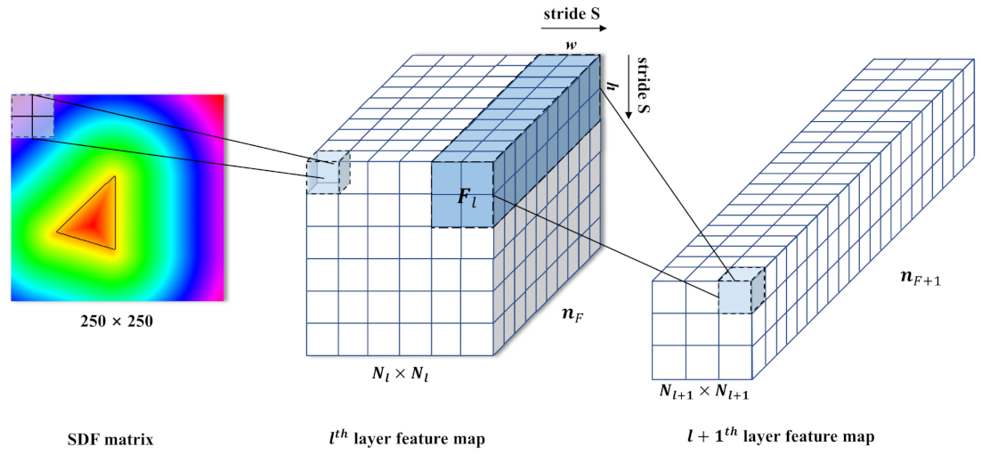
Figure 4.
Schematic of the convolution operation. The light blue matrix denotes a 2 × 2 convolutional kernel, and the white matrix represents the feature map.
Figure 4.
Schematic of the convolution operation. The light blue matrix denotes a 2 × 2 convolutional kernel, and the white matrix represents the feature map.
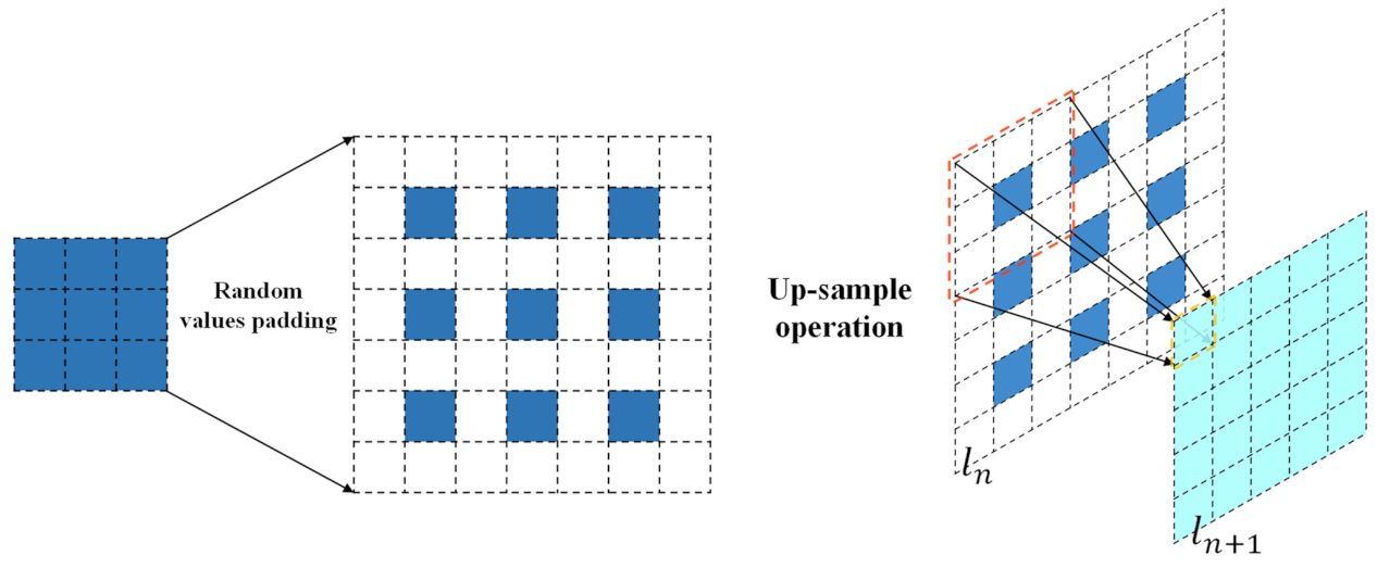
Figure 5.
Schematic of the deconvolutional layer: the dark blue block represents the feature map at the
layer, the white block illustrates the padding location of the layer’s feature map, and the pool blue block represents the feature map at the next layer ().
Figure 5.
Schematic of the deconvolutional layer: the dark blue block represents the feature map at the
layer, the white block illustrates the padding location of the layer’s feature map, and the pool blue block represents the feature map at the next layer ().
Figure 6.
Geometry of the objects of the validation dataset: (a) Car, (b) Car2, (c) Airplane, (d) Locomotive, (e) Ship, (f) Submarine, (g) Bionic Fish, (h) Missile.
Figure 6.
Geometry of the objects of the validation dataset: (a) Car, (b) Car2, (c) Airplane, (d) Locomotive, (e) Ship, (f) Submarine, (g) Bionic Fish, (h) Missile.
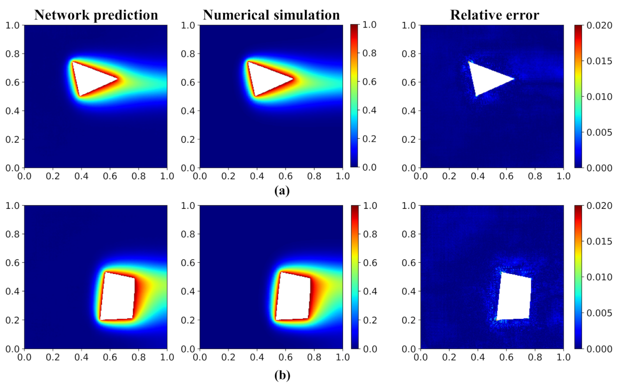
Figure 7.
Temperature field and error distribution of validation cases. (a) Triangle and (b) quadrangle. The first and second columns show the temperature field predicted by the network model and the numerical simulation (OpenFOAM). The third column shows the relative error distribution.
Figure 7.
Temperature field and error distribution of validation cases. (a) Triangle and (b) quadrangle. The first and second columns show the temperature field predicted by the network model and the numerical simulation (OpenFOAM). The third column shows the relative error distribution.
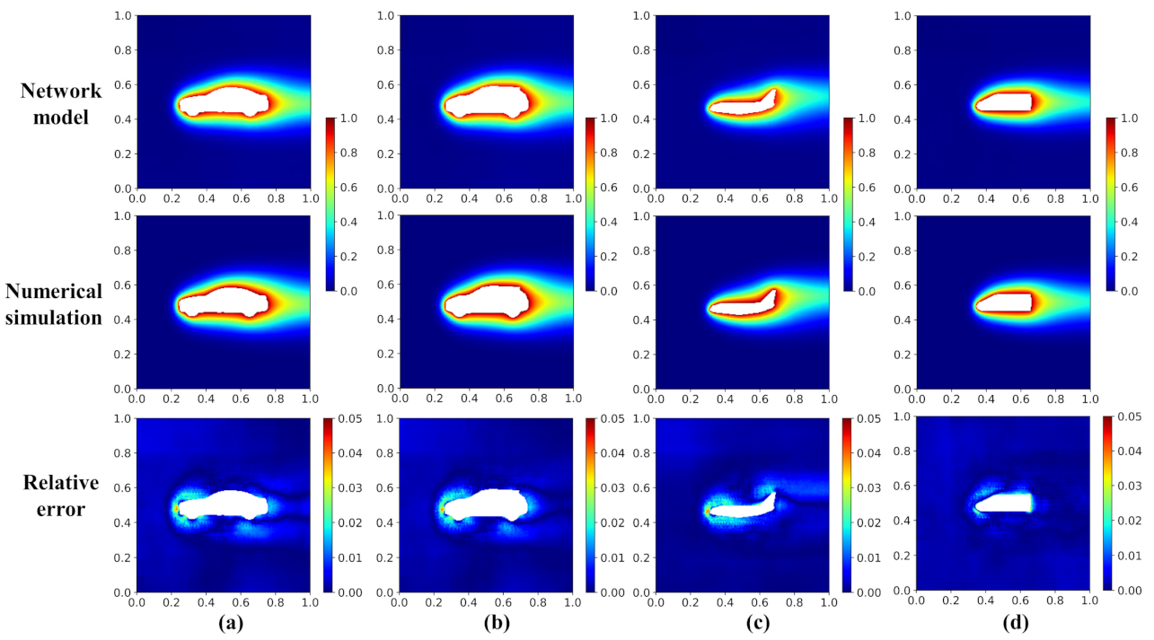
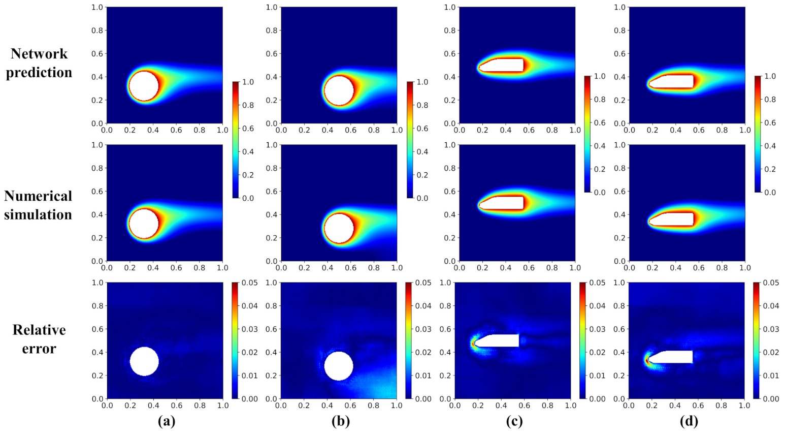
Figure 8.
Temperature field and relative error distribution of the validation cases with the geometries of (a) Car, (b) Car2, (c) Airplane, and (d) Locomotive.
Figure 8.
Temperature field and relative error distribution of the validation cases with the geometries of (a) Car, (b) Car2, (c) Airplane, and (d) Locomotive.
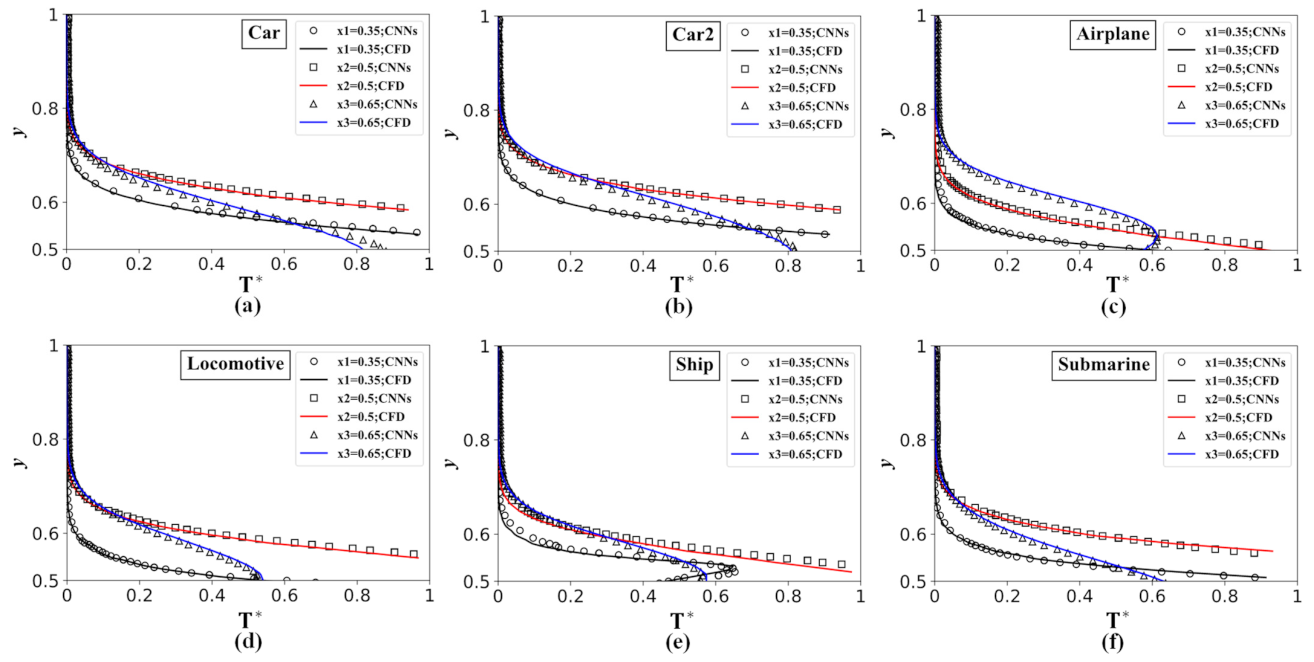
Figure 9.
Dimensionless temperature profiles of the validation case distribution along the y-direction at
= 0.35, = 0.5, and = 0.65 by the network model (symbols) and numerical simulation (lines): (a) Car, (b) Car2, (c) Airplane, (d) Locomotive, (e) Ship, (f) Submarine.
Figure 9.
Dimensionless temperature profiles of the validation case distribution along the y-direction at
= 0.35, = 0.5, and = 0.65 by the network model (symbols) and numerical simulation (lines): (a) Car, (b) Car2, (c) Airplane, (d) Locomotive, (e) Ship, (f) Submarine.
Figure 10.
Velocity field and error distribution of the testing cases. (a) Quadrangle and (b) Pentagon. The first and second columns are the fields predicted by the network model and the numerical simulation (OpenFOAM), respectively. The third column shows the relative error distribution.
Figure 10.
Velocity field and error distribution of the testing cases. (a) Quadrangle and (b) Pentagon. The first and second columns are the fields predicted by the network model and the numerical simulation (OpenFOAM), respectively. The third column shows the relative error distribution.
Figure 11.
Velocity field and relative error distribution of the validation cases with the geometries of Car, Car2, Airplane, Locomotive, Ship, and Submarine.
Figure 11.
Velocity field and relative error distribution of the validation cases with the geometries of Car, Car2, Airplane, Locomotive, Ship, and Submarine.
Figure 12.
Max (
) and mean () relative prediction error on the velocity field by the network model for various validation objects.
Figure 12.
Max (
) and mean () relative prediction error on the velocity field by the network model for various validation objects.
Figure 13.
Convergence history of the network models with different structures of the network.
Figure 13.
Convergence history of the network models with different structures of the network.
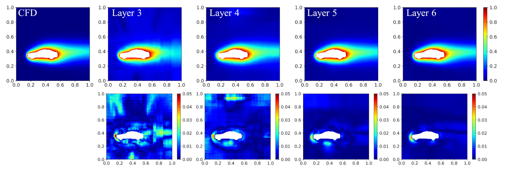
Figure 14.
Predicted temperature field obtained using different network structures. The top row is the predicted field by the network model and the CFD; the second row is the corresponding error distribution.
Figure 14.
Predicted temperature field obtained using different network structures. The top row is the predicted field by the network model and the CFD; the second row is the corresponding error distribution.
Figure 15.
Temperature distribution predicted by the network model and numerical simulation with different positions of the hot objects and the corresponding relative error: (a) left circle, (b) down circle, (c) left locomotive, (d) lower left locomotive.
Figure 15.
Temperature distribution predicted by the network model and numerical simulation with different positions of the hot objects and the corresponding relative error: (a) left circle, (b) down circle, (c) left locomotive, (d) lower left locomotive.
Figure 16.
Temperature fields of the case with two circles predicted by the network model and numerical simulation and the corresponding relative error.
Figure 16.
Temperature fields of the case with two circles predicted by the network model and numerical simulation and the corresponding relative error.
Figure 17.
Max () and mean () relative prediction error on the temperature field by the network models with and without incorporating the velocity field as part of the input matrices. The blue bar denotes the cases without velocity information, and the red bar denotes the cases with velocity information.
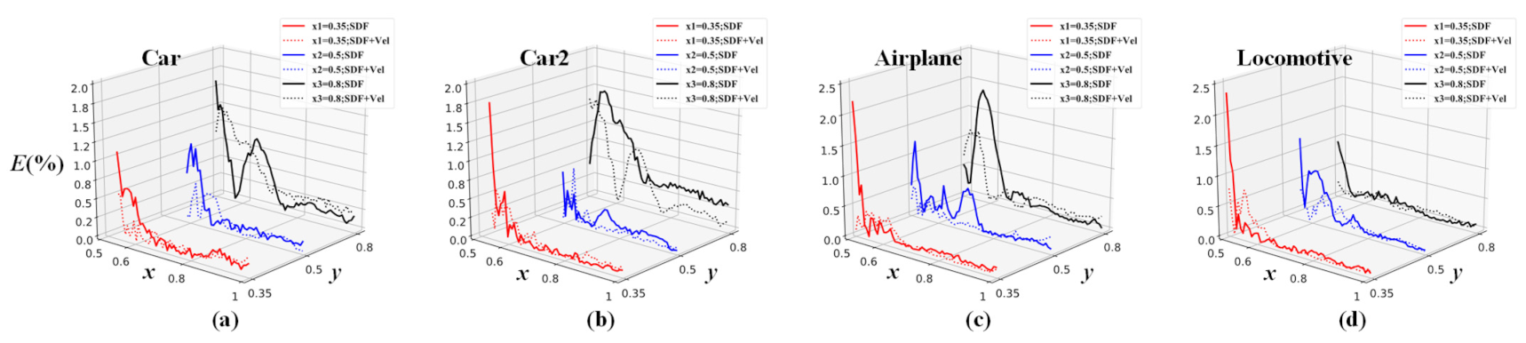
Figure 18.
Relative error profile along the y-direction at
= 0.35, = 0.5, and = 0.8. The studied validation cases are (a) Car, (b) Car2, (c) Airplane, and (d) Locomotive.
Figure 18.
Relative error profile along the y-direction at
= 0.35, = 0.5, and = 0.8. The studied validation cases are (a) Car, (b) Car2, (c) Airplane, and (d) Locomotive.
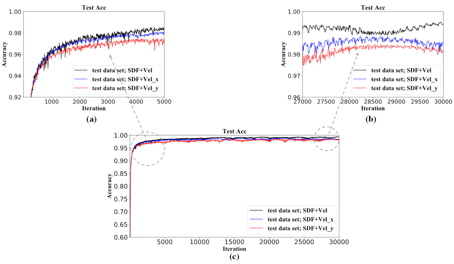
Figure 19.
Training/convergence history of the network models: (a) local magnification in iteration from 0 to 5000; (b) local magnification in iteration from 27,000 to 30,000.
Figure 19.
Training/convergence history of the network models: (a) local magnification in iteration from 0 to 5000; (b) local magnification in iteration from 27,000 to 30,000.
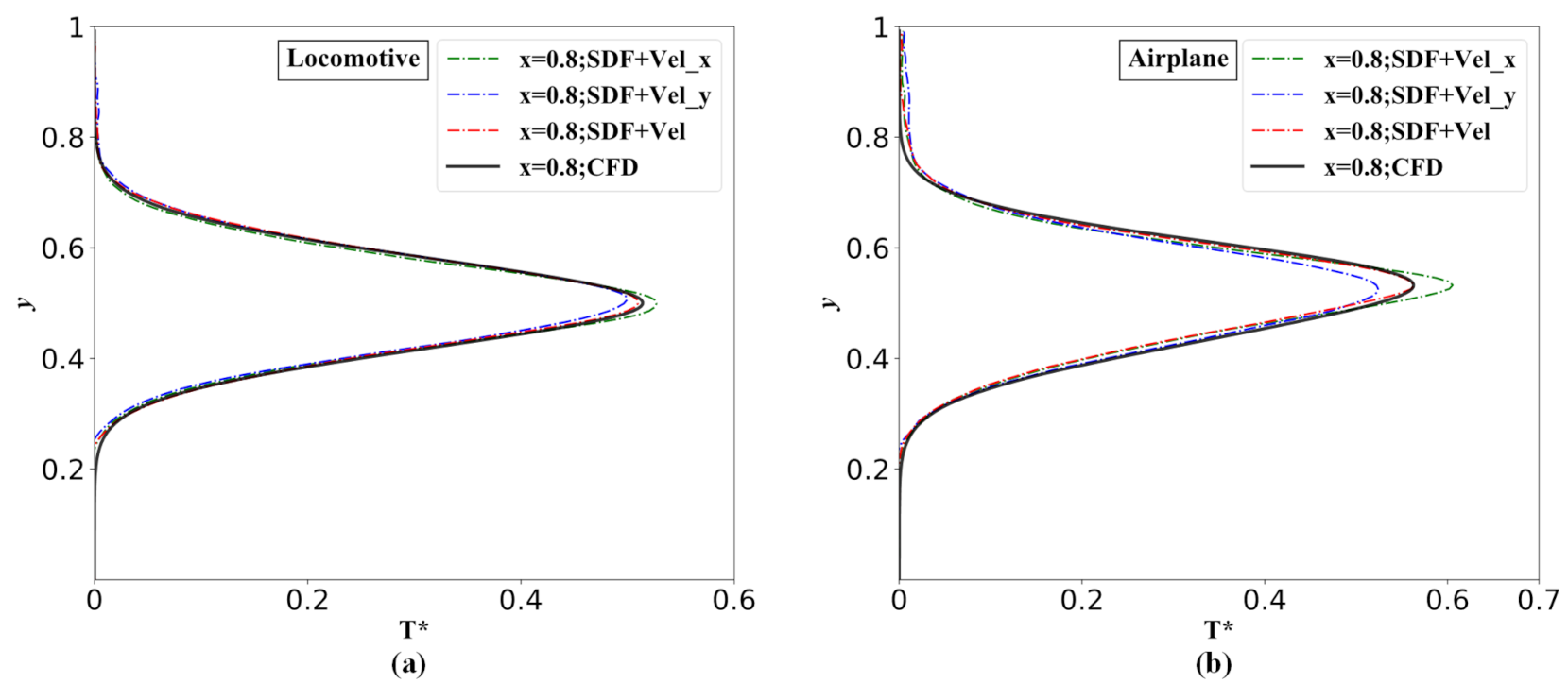
Figure 20.
Dimensionless temperature profiles of the validation case distribution along the y-direction at
= 0.8 by the network model with different input matrices and numerical simulations: (a) Locomotive and (b) Airplane.
Figure 20.
Dimensionless temperature profiles of the validation case distribution along the y-direction at
= 0.8 by the network model with different input matrices and numerical simulations: (a) Locomotive and (b) Airplane.
Table 1.
Parameters of the neural network model of each layer, where
denotes the size of the convolution kernel (F), denotes the number of F, and is the size of the lth layer after operation.
Table 1.
Parameters of the neural network model of each layer, where
denotes the size of the convolution kernel (F), denotes the number of F, and is the size of the lth layer after operation.
| Name of Layer | Executing Operation
| Shape
|
|---|
| Input of model | -- | 250 × 250 × 1 |
| Conv1 | 4 × 4 × 32/3 | 83 × 83 × 32 |
| Conv2 | 5 × 5 × 64/2 | 40 × 40 × 64 |
| Conv3 | 6 × 6 × 128/2 | 18 × 18 × 128 |
| Conv4 | 6 × 6 × 256/2 | 7 × 7 × 256 |
| Conv5 | 3 × 3 × 512/2 | 3 × 3 × 512 |
| Conv6 | 2 × 2 × 1024/1 | 2 × 2 × 1024 |
| Conv7 | 1 × 1 × 1024/1 | 2 × 2 × 1024 |
| Deonv1 | 2 × 2 × 1024/1 | 3 × 3 × 1024 |
| Deonv2 | 3 × 3 × 512/2 | 7 × 7 × 512 |
| Deonv3 | 6 × 6 × 256/2 | 18 × 18 × 256 |
| Deconv4 | 6 × 6 × 128/2 | 40 × 40 × 128 |
| Deconv5 | 5 × 5 × 32/2 | 83 × 83 × 32 |
| Output | 4 × 4 × 1/3 | 250 × 250 |
Table 2.
Hyperparameters of the optimization algorithm. Regularization coefficient () and learning rate ().
Table 2.
Hyperparameters of the optimization algorithm. Regularization coefficient () and learning rate ().
| Hyperparameter | Value |
|---|
| Batch size | 64 |
| 0.0001 |
| 0.00008 |
Table 3.
Boundary conditions of the numerical model.
Table 3.
Boundary conditions of the numerical model.
| Boundary Type | Temperature | Velocity | Pressure |
|---|
| Wall | Fixed value | Fixed value | Zero gradient |
| Inlet | Fixed value | Fixed value | Zero gradient |
| Outlet | Zero gradient | Zero gradient | Fixed value |
| Object | Fixed value | Fixed value | Zero gradient |
Table 4.
Average temperature at the outlet (Ot) with different meshes.
Table 4.
Average temperature at the outlet (Ot) with different meshes.
| Mesh | Grid Number | Outlet Temp (Ot) |
|---|
| Grid-one | 8849 | 311.4296 |
| Grid-two | 18,786 | 311.3324 |
| Grid-three | 25,068 | 311.2711 |
| Grid-four | 31,514 | 311.2264 |
Table 5.
Time consumption for predicting the steady-state temperature field by the network model (GPU, 2080ti) and the numerical simulation (CPU, Ryzen 7 3700X, OpenFOAM).
Table 5.
Time consumption for predicting the steady-state temperature field by the network model (GPU, 2080ti) and the numerical simulation (CPU, Ryzen 7 3700X, OpenFOAM).
| Geometry Object | CNNs (s) | OpenFOAM (s) | Grid Quantity | Speedup |
|---|
| Car | 0.2354 | 38 | 10,144 | 161 |
| Car2 | 0.2423 | 31 | 10,000 | 128 |
| Airplane | 0.2314 | 23 | 9032 | 99 |
| Locomotive | 0.2284 | 20 | 7758 | 88 |
| Bionic Fish | 0.2463 | 28 | 8252 | 114 |
| Missile | 0.2324 | 26 | 8528 | 112 |
| Ship | 0.2364 | 22 | 8956 | 93 |
| Submarine | 0.2394 | 26 | 9876 | 109 |
Table 6.
Time consumption for predicting the steady-state temperature field by the network model on GPU 1660s and GPU 2080ti.
Table 6.
Time consumption for predicting the steady-state temperature field by the network model on GPU 1660s and GPU 2080ti.
| Geometry Object | 1660s Time (s) | 2080ti Time (s) |
|---|
| Car | 0.3983 | 0.2354 |
| Car2 | 0.3723 | 0.2423 |
| Airplane | 0.3523 | 0.2314 |
| Locomotive | 0.3793 | 0.2284 |
| Bionic Fish | 0.3194 | 0.2463 |
| Missile | 0.3164 | 0.2324 |
| Ship | 0.317 | 0.2364 |
| Submarine | 0.3184 | 0.2394 |
Table 7.
Average relative error () on the prediction of the testing and validation datasets by the network models using the SDF and binary image representation.
Table 7.
Average relative error () on the prediction of the testing and validation datasets by the network models using the SDF and binary image representation.
| Datasets | Prediction Field | SDF | Binary |
|---|
| Testing | Velocity | 2.79% | 6.56% |
| Temperature | 0.83% | 4.62% |
| Validation | Velocity | 5.12% | 18.27% |
| Temperature | 1.91% | 10.82% |
Table 8.
Parameters memory, training time, and prediction time costs for the network model with different numbers of layers.
Table 8.
Parameters memory, training time, and prediction time costs for the network model with different numbers of layers.
| Layer | Parameters Memory (MB) | Prediction Time (s) | Training Time (min) |
| 3 | 7.23 | 0.1197 | 43.2 |
| 4 | 31.7 | 0.1497 | 51.1 |
| 5 | 58.7 | 0.1825 | 64.4 |
| 6 | 247 | 0.2643 | 86.3 |


