Abstract
The instability of surface lenticular vortices is investigated using a comprehensive suite of laboratory experiments combined with numerical linear stability analysis as well as nonlinear numerical simulations in a two-layer Rotating Shallow Water model. The development of instabilities is discussed and compared between the different methods. The linear stability analysis allows for a clear description of the origin of the instability observed in both the laboratory experiments and numerical simulations. While global qualitative agreement is found, some discrepancies are observed and discussed. Our study highlights that the sensitivity of the instability outcome is related to the initial condition and the lower-layer flow. The inhibition or even suppression of some unstable modes may be explained in terms of the lower-layer potential vorticity profile.
1. Introduction
Mesoscale vortices are a major component of the global oceanic circulation. They are particularly common in oceanic regions of high mesoscale activity and can have long lifetimes, up to the order of a year (e.g., [1,2,3,4]). These coherent structures play an active role in the energetics of the ocean general circulation, in the transport of biological species, heat and salt anomalies, and in air–sea interaction (e.g., [5,6]). For example, eddies that detach from currents separating oceanic regions with different properties may propagate from one side to the other, transporting into a new region water with anomalous properties. These warm- and cold-core vortices are associated with the intersection of the isopycnals with the surface of the ocean, forming a front (e.g., [7]), but can also be sub-surface intensified [8] or form lenticular vortices at depth, a well known example of such vortices being the meddies [3]. Typical eddy size in the ocean are a few Rossby deformation radii (between 1 and 5 for eddies described in details in the literature), with Rossby numbers smaller than unity but finite (typically below in absolute value) (e.g., [4,9,10,11]). Smaller eddies can also be found, down to the submesoscale and with higher Rossby numbers (e.g., [12,13]). Warm-core surface anticyclonic vortices are the subject of this study and will be referred as lenticular vortices.
Early modelling studies of the dynamics of such vortices date back to the 1970s, starting with experimental studies [14,15]. Subsequently Griffiths and Linden [16] performed laboratory experiments in a rotating tank, using two different methods for generating the vortex. The first method (referred to as constant-flux) consists of slowly injecting a lighter fluid at the surface of the tank filled with heavier fluid until the desired volume for the vortex is obtained (this technique was already used by Gill et al. [15]). The second technique, the so-called constant-volume method previously used by Saunders [14], consists of releasing a given volume of lighter fluid initially contained in a suspended cylinder. Under the action of buoyancy and rotation, the patch of lighter fluid adjusts towards an axisymmetric vortex which eventually destabilizes and breaks up.
The issue of the stability of oceanic surface vortices has also been addressed in theoretical and numerical studies. The (multi-layer) Rotating Shallow Water (RSW) model has been widely used to investigate their dynamics, representing the eddies as patches of lighter fluid overlying a deep ocean. Such model is appealing because it allows for an explicit representation of the density anomaly (compared to the exterior region) in the eddy, as well as the outcropping of the isothermal or isopycnal (e.g., [7,17]). This outcropping can be associated with specific dynamical features (including instabilities) associated with the frontal configuration [18,19,20]. In the two-layer configuration, Ripa [21] derived a semi-analytical criterion for the instability of vortices in solid-body rotation. He classified the instability regimes in terms of wave-wave resonances, showing that lenticular vortices with constant (zero in their case) Potential Vorticity (PV) over a quiescent layer of fluid are prone to instability through resonance between a Poincaré-like wave in the upper layer and a Rossby wave in the lower layer, for realistic oceanic eddy size and intensity. Paldor and Nof [22] investigated numerically the linear stability of zero-PV lenticular vortices and found unstable modes with azimuthal wavenumber . More recently, Cohen et al. [23] extended this analysis to vortices with constant non-zero PV.
The fact that eddies with very long lifetimes are observed seems to conflict with results from these idealized studies, which found instability for typical oceanic regimes. Part of the explanation could be related to the flow surrounding the vortex, and in particular to the circulation below it. Dewar and Killworth [24] showed (although not in the context of lenticular vortices) that a co-rotating flow under an eddy decreases the growth rate of the instability, and Benilov [25] showed that a constant-PV lower-layer flow suppresses baroclinic instability in a QG model, the explanation being that Rossby wave propagation is precluded in the lower layer in such a configuration. In a two-layer RSW model, Cohen et al. [26] also reported no finding of unstable mode for lenticular vortices over a constant PV layer.
While the nonlinear development of the instability of isolated but non-outcropping vortices (i.e., vortices surrounded horizontally by a ring of opposite-signed vorticity) has been investigated numerically in numerous papers, either in layered or continuously stratified models (e.g., [27,28,29,30,31]), few simulations of the evolution of lenticular vortices have been reported to our knowledge. Verzicco et al. [32] reproduced the constant-volume experiments of Griffiths and Linden [16] and the subsequent evolution of the vortex for a few cases, using numerical simulation of the Boussinesq equations. Numerical simulations of the two-layer shallow water equations were performed by Thivolle-Cazat et al. [33]. They used the MICOM code in conjunction with data assimilation of laboratory experiments measurements (on the Coriolis platform in Grenoble, France). They did not focus on lenticular vortices, which represented only 5 runs out of experiments. This rather scarce number of numerical studies is partly due to the difficulty of having a reliable numerical scheme for the shallow water equations that deals with the outcropping of one of the layers. On the other hand, fully three-dimensional numerical simulations still require large computational resources, making a large number of runs with different parameters at high resolution impractical.
In this paper, we report results on the instability of constant-PV surface lenticular vortices in a two-layer configuration. These results are based on laboratory experiments covering a wide range of vortex parameters (aspect ratio and PV), supplemented by extensive nonlinear numerical simulations of the two-layer RSW equations. These are compared to results from a linear stability analysis using the latter model. Besides allowing to capture outcropping and related frontal dynamics, the two-layer model is very close to the experimental setup used in this study, thus allowing for a more accurate comparison. A description of the model equations and methods, including the laboratory experiments setup, the nonlinear numerical simulation code and the linear stability analysis, are given in Section 2. In Section 3, we discuss the linear stage of the developing instability observed in both the nonlinear numerical simulations and laboratory experiments, and compare to results from the linear stability analysis. Then Section 4 addresses the nonlinear saturation of the instability, mostly in the numerical simulations, and contains a detailed analysis of one run illustrating the dynamics. A discussion on the impact of a lower layer flow is provided in Section 5, and conclusions are presented in Section 6.
2. Problem Formulation and Methods
2.1. RSW Equations and Basic State
2.1.1. The Two-Layer RSW Model
The two-layer RSW equations in polar coordinates are, e.g., [34]
where i is the index of the layers (1 and 2 for the upper and lower layer, respectively), the Lagrangian derivative, the horizontal velocity, the pressure and the layer thickness. This system of equations is supplemented by a dynamical condition at the interface:
In the following, we will use either the rigid lid assumption, which implies with a constant corresponding to the nondimensional total thickness of fluid at rest (see below for the nondimensionalization); or a free-surface upper boundary condition. The rigid lid assumption allows for a simpler discussion of the formulation of the linear stability analysis and the spectra of unstable modes, while capturing the essential mechanisms at play in both the laboratory experiments and the nonlinear numerical simulation.Relaxing this approximation yields additional unstable modes that mostly take place for non-realistic dynamical parameters, as will be discussed separately.
We shall consider here the stability of surface lenticular vortices and nondimensionalize the equations accordingly. We use the size of the eddy (i.e., the radius of outcropping of the interface) as the typical horizontal length scale and the inverse Coriolis parameter as a typical time scale. The velocity is non-dimensionalized by (i.e., the nondimensional velocity is the Rossby number ). The thickness is non-dimensionalized with the value associated with a baroclinic (or rather upper-layer) deformation radius equal to the size of the vortex: , where is the reduced gravity. That is, the depth scale used for non-dimensionalization is and, correspondingly, the pressure scale is . The barotropic Burger number of the vortices investigated is given by and is large (greater than 10 for most experiments, the minimal value being 3), justifying the use of the rigid lid approximation for the linear stability analysis.
2.1.2. Vortex Profiles
Lenticular vortices are steady axisymmetric solutions of the equations with zero radial velocity and azimuthal velocity obeying cyclogeostrophic balance. They satisfy in each layer the following system of (nondimensional) equations:
which is valid both for the free-surface and the rigid lid upper boundary conditions (the difference arising in the relationship between and ). In the notation used in this paper, upper-case variables stand for background state whereas lower case are for perturbations (and for some parameters). The family of upper-layer profiles we consider is defined by a constant value of potential vorticity . This aims at reproducing the profiles obtained in a constant-volume experiment, where some fluid initially contained in a bottomless cylinder is released and adjusts through the combined action of Coriolis and buoyancy forces. The PV of the upper layer, initially contained in the cylinder, is constant with , (with the initial thickness of the upper layer fluid contained in the cylinder) and nearly remains so throughout the adjustment and subsequent evolution. This assumption of constant upper PV is also relevant for typical oceanic profiles [7,9]. In the lower layer, we will primarily consider two different situations: (quiescent lower layer, with ), which is the most trivial solution, and piecewise constant. The latter configuration aims at capturing more accurately the profile obtained in constant-volume experiments. This method consists of releasing a volume of buoyant fluid initially contained in a suspended cylinder at the center of a rotating tank. The fluid initially below the cylinder in the lower layer has a positive PV anomaly, so that PV has a piecewise-constant distribution. In the course of the adjustment, this volume of fluid slightly shrinks inward and acquires a weak cyclonic circulation. The lower layer PV is then given by
where is the location of fluid parcels that were initially at the radius of the cylinder before adjustment. With the rigid lid approximation, the momentum equations for the background state (4) in each layer reduce to:
Equations (5) and (7) come with the boundary conditions and , . In the lower layer at , as mass conservation implies that fluid parcels in the lower layer at are unaffected during the adjustment. The resulting boundary-value problem is solved numerically with a standard boundary value problem solver, using a linear expansion for near the singularity at of the form . Examples of vortex profiles with different values of are given in Figure 1.
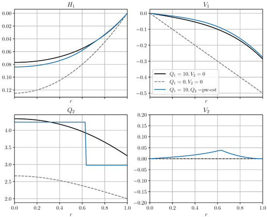
Figure 1.
Basic vortex profile: nondimensional upper-layer thickness (upper left panel), lower-layer PV (lower left panel) and upper and lower layer azimuthal velocity and (upper and lower right panels, respectively). The vortex parameters are , , and the solution with a quiescent lower layer (black) is compared to the solution with a piecewise-constant lower-layer PV (blue). The analytical solution for , is plotted as a grey dashed line for reference.
2.1.3. Range of Parameters Investigated and Estimates of Realistic Values
Typical dynamical parameters for major ocean eddies, such as the Gulf Stream or Agulhas rings, were reported in (e.g., Olson [2], Goni et al. [11]), sometimes with an interpretation based on a two-layer formulation [10,35]. In the latter study, the authors reported typical values for two Agulhas rings of 400 m for the vertical displacement of the isopycnal, in the range 110 km–130 km and maximum absolute azimuthal velocity in the range 0.6 m/s–0.9 m/s. The deformation radius is of the order of 30 km in this area [36] (computing , with m/s2 as reported by the authors, gives the same value). The resulting Burger number ranges between and , while the Rossby number is between around and . These typical dynamical parameters were confirmed by observations from satellites in ths region [11], who reported typical eddy size ranging from 50 km–170 km.
For a Gulf stream warm core ring (82B), the reported values were around 500 m for the isothermal displacement, around m/s and 60 km. The deformation radius is around 20 km in this region, so the typical Burger number is around , as well as the typical Rossby number.
In our scaling, the potential vorticity (at the center of the vortex, and assuming it is constant)
and is thus equal to the inverse Burger number in the limit of small Rossby number. Therefore, the nondimensional PV associated with the above-mentionned eddies ranges between 9 and 20. More generally, sizes of ocean rings range between 1 and 5 deformation radius [2], so that and . Typical realistic values of do not exceed . Of course, smaller eddies with larger Rossby numbers are known to exist (e.g., [4,13]), and these would have smaller values of (as well as ).
2.2. Methods
2.2.1. Setup of the Laboratory Experiments
Lenticular vortices were produced through the adjustment of a buoyant fluid initially confined in a bottomless cylinder in a rotating tank, the so-called constant-volume experimental setup [16,37]. The mechanical lift-up of the inner cylinder, which is co-aligned with the rotation axis of the tank, was triggered after the water in the tank had reached solid-body rotation. A schematic of the experimental setup is given in Figure 2.
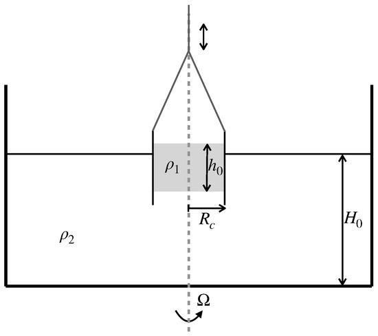
Figure 2.
Schematics of the laboratory experiment setup, showing the rotating tank and the inner cylinder with lighter fluid inside, before removal.
The rotating tank was a square with side 99 cm and depth 51 cm. The rotation rate could be varied between rad s−1 and rad s−1 within an accuracy of . We used two different cylinders with radius cm and 20 cm. Dyed fresh water was used to visualize the evolution of the vortex using a CCD camera placed above the tank. The lower layer was salt water with concentration in the range 3.6–80 , thus setting the value of the reduced gravity. The total fluid depth was varied from 8–40 while the thickness of lighter fluid in the cylinder was cm, covering a range of initial depth ratio . In total, 42 different experiments were performed, with initial Burger numbers varying between and . A table summarizing the parameters of the laboratory experiments is given in Appendix D.
We relate these values to the nondimensional values of the potential vorticity and aspect ratio . This is done using the semi-empirical fact that the vortex spreads out by approximately one baroclinic deformation radius, , during the initial adjustment, as was noticed by Griffiths and Linden [16], so that . Thus, the nondimensional upper-layer PV becomes:
For the depth ratio we use the qualitative formulas given by Griffiths and Linden [16]:
Formulas (9) and (10) are used to infer the vortex parameters in the laboratory experiments, allowing for a comparison with the nonlinear numerical simulations and results from the linear stability analysis.
2.2.2. Linear Stability Analysis
For comparison with observations from laboratory experiments and nonlinear numerical simulations, we perform a linear stability analysis of the base flow described above. For simplicity, and since it does not affect the main results, we use the rigid-lid approximation here – extension to the free surface case is discussed in Appendix C. The nondimensional equations are linearized around the basic state using the standard normal mode decomposition , introducing an additional change of variable for convenience. This gives the linear eigenproblem for the eigenvalue defined for :
Boundary conditions for this problem are regularity of the solution at and . In the exterior domain (), the rigid lid condition enforces a non-divergent flow–cf. (13)–with . The flow in the exterior region can be obtained analytically, using a condition of decay as . This leads to boundary conditions at for the interior solution (see Appendix A for details):
The resulting eigenproblem is solved using a collocation method with Chebyshev polynomials. Regularity of the solution is ensured by the form of the interpolants. The azimuthal momentum and mass conservation equations are multiplied by r for the numerical implementation. Numerical convergence in the case of an eddy over a quiescent lower layer is reached for resolutions as low as 10 points.
2.2.3. Nonlinear Simulations: Numerics and Initial Conditions
For the nonlinear simulations, we used a high-resolution finite-volume numerical code [38]. It integrates the two-layer RSW Equations (1) and (2) with a free surface in conservative form, using a well-balanced entropy-satisfying scheme. The latter ensures physically appropriate behavior in cases of shock formation (namely a decrease in energy) without requiring explicit dissipation. In this regard, the numerical code belongs to the family of implicit Large Eddy Simulation (iLES). In particular, it copes well with outcropping (vanishing layer thickness), which is required for the simulation of lenticular vortices. This code was previously used in the context of frontal dynamics by, e.g., Gula et al. [18], Ribstein and Zeitlin [19], Gula and Zeitlin [39]. The numerical simulations are initialized using the solutions for the lenticular vortices considered in Section 2.1.2, with a quiescent lower layer, adapted to the free surface condition and suitably perturbed to trigger the instability. The perturbation is obtain by applying a -dependent map to the radial variable when computing the solution , as described in Appendix B. A weak radial velocity field is then computed so that the divergence of the velocity vanishes, in order to limit the generation of ageostrophic motions and especially of inertia-gravity waves. The azimuthal wavenumbers of the perturbation range from 2 to 10 (unless otherwise stated), and the perturbation’s relative magnitude is of the order of a few percent. A series of numerical experiments were carried out to span the plane. Values used in the initial conditions are given in Table 1. The size of the domain is four time the diameter of the vortices, and the numerical grid has points.

Table 1.
Values of the parameters and used in the initial conditions of the numerical simulations (every pairs).
3. Early Stage of the Instability
In this section, we report the behavior of the vortices at early stages of the instability from the laboratory experiments and nonlinear simulation and compare it with the results from the linear stability analysis.
3.1. Preliminary Considerations from Linear Stability Analysis
We first briefly discuss the results from the linear stability analysis, neglecting the background current () for simplicity. A diagram of the wavenumber m and growth rate of the most unstable mode in the plane is given in Figure 3. An extensive discussion of the linear stability of these kind of vortices can be found in (Cohen et al. [23], their “regular” regime).
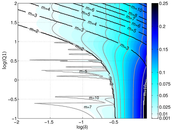
Figure 3.
Growth rate (colours) and wavenumber (black contours) of the most unstable mode, as found from the linear stability analysis, in the parameter space, for lenticular vortices with a quiescent lower layer (). Following the discussion of realistic parameters (see Section 2.1.3), typical values for large ocean rings are and .
Instability is found for large values of the aspect ratio and/or the potential vorticity , with the wavenumber of the most unstable mode increasing with both of these parameters, while the growth rate depends predominantly on . The latter dependence is in agreement with what was found for non-outcropping eddies in two-layer models (e.g., [24,40]). From the wave resonance point of view, the “standard” unstable modes (in the upper and rightmost part of the diagram) result from the interaction between a frontal-type wave in the upper layer, sometimes referred to as a mixed Rossby-Poincaré or Yanai mode, and a Rossby wave in the lower layer [18,21,23,39]. The latter is supported by the presence of the PV gradient associated with the slope of the interface since the lower-layer PV is given by . The growth rate thus depends on the efficiency of the mutual amplification between the upper- and lower-layer waves, which is primarily driven by their spatial structure (the shape of the modes) and their phase speed difference, as phase-locking is a necessary condition for mutual amplification. A review of two-layer and frontal instabilities is given in Zeitlin [34].
There is a zone of relative stability in the lower-left corner of the diagram, delimited by the contour. In this region, however, small zones of instability also exist with rather high () wavenumbers and growth rates not exceeding . These instabilities involve higher radial wavenumber Poincaré modes in the upper layer. The latter have different phase speed, therefore experiencing phase locking for different (higher) values of the azimuthal wavenumber compared to the unstable modes described above. Finally, one sees a weak region of very high growth rate (up to ) with wavenumber for very large depth ratio () and weak , which we identify as a frontal-frontal (i.e., implying a Rossby-Poincaré wave in the lower layer instead of a Rossby wave) instability [19].
3.2. Observations in Laboratory Experiments
Just after the withdrawal of the cylinder, the freshwater spreads radially and the flow adjusts to an axisymmetric lenticular vortex. The detailed dynamics of this initial adjustment has been carefully discussed in several papers [16,33,37] and is not the subject of the current paper. One should keep in mind that dissipative processes and mixing occur, especially close to the edge of the vortices, diminishing the azimuthal velocity and reducing the shear between the two layers there [37]. This is almost certainly the main source of differences between the experimental adjusted lenticular vortex profile and the inviscid solution. After this period, the flow eventually starts to develop non-axisymmetric features that consist of m arms developing out of the initial vortex and rolling up in a cyclonic sense, forming dipolar structures that can eventually detach and propagate away.
Snapshots of different stages of the initial adjustment and the development of an instability with are shown in Figure 4. The parameters of this eddy (see table in Appendix D) are . That is a very large eddy (around 7 deformation radii) with a Rossby number of order . Here and below, when restoring dimensional values, we will use 25 km and , which is fairly typical of mid-latitudes. Using these, the maximum velocity is m/s, which is large (but one should keep mind that all these parameters are estimated within at least a factor of 2 uncertainty). In the laboratory experiments, the number of arms is often well defined and their development rates are of the same order. Sometimes, at high-wavenumber, one or two arms may have an inhibited growth compared to the others (see Figure 4d). The wavenumber of the developing unstable mode, as well as the timescale of the growth of the instability, are different between the various experiments ( for the investigated range of parameters). A comparison of the prediction from the linear stability analysis with the experimental observations is given in Figure 5 (left panel) and shows good agreement. Possible reasons for the observed discrepancies are the following:
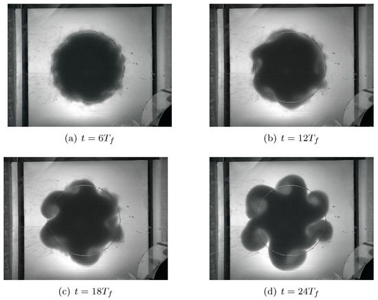
Figure 4.
Snapshots of the evolution of the flow during a developing instability with wavenumber observed in the laboratory experiment. Small-scale dissipative processes during the initial adjustment are visible in the first snapshot. Estimated eddy parameters are , .
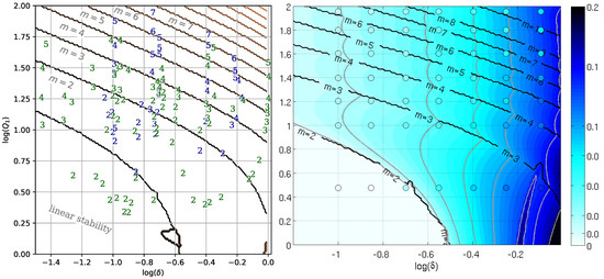
Figure 5.
Left panel: wavenumbers of the most unstable modes from the linear stability analysis (contours) and observed in laboratory experiments (text). Green labels are reproduced from (Griffiths and Linden [16], their Figure 5), and blue labels are from our set of experiments. Contours in the lower left part of the panel has been removed for visibility, using the condition for modes higher than in this region of the space. Right panel: comparison of the growth rate predicted by linear theory (colours) and measured in the numerical experiments (colored bullets) in the parameter space (zoomed over the range of values investigated in the nonlinear simulations).
- The parameters in the laboratory experiments are deduced from qualitative considerations and semi-empirical relations, neglecting the details of the initial adjustment;
- Friction effects decreases the azimuthal velocity, especially during the initial adjustment and near the edge of the eddy [37].
- The initial adjustment leaves out high-wavenumber perturbations to the vortex before the instability starts developing (see Figure 4a). The vortex may be unstable with respect to several wavenumbers, which are unevenly excited by this perturbation, so that a mode that is not the most unstable may initially gain more energy than the most unstable one and develop faster.
Another possible source of differences is that the lower-layer flow is neglected in the linear stability analysis. However, as will be shown in Section 5, this is very unlikely to be the dominant cause of discrepancies.
3.3. Results from Nonlinear Numerical Simulations
Our numerical simulation reproduces the observations reported previously from the laboratory experiments, as far as the development of the instability is concerned, at least qualitatively. We compute a growth rate associated with the development of the instability based on the perturbation of the upper layer thickness with respect to the angular mean at the initial time. A clear period of linear growth is observed in every simulation. Figure 5 (right panel) shows a comparison of the growth rate calculated in the numerical simulations and that predicted by the linear stability analysis here adapted to the free surface for a more rigorous comparison. Note that, for the range of investigated, the impact of the free surface compared to a rigid lid approximation is negligible (see Appendix C for an extended discussion).
Rather good agreement is found in most cases. In particular, no instability occurs for the two runs outside the linear instability zone and the growth rate of the most unstable mode increases with the depth ratio and to some extent with the upper layer PV. Nonetheless, the growth rate measured in numerical simulations is systematically smaller that the linear prediction, with a relative error ranging between 10% and 40% and roughly increasing with . Several explanations are possible for this discrepancy. It is most likely because of numerical dissipation near the edge of the vortex: although the numerical code does not use explicit viscosity, the entropy condition used in the Riemann solver is associated with a decrease of the energy across shocks. Hence, energy dissipation occurs at the edge of the lens. In addition, there is a non-negligible time before the unstable mode starts developing, because the initial amplitude of the perturbation is weak and the shape of the perturbation is different from that of the unstable modes. Short-time non-normal modes are very likely to be excited by such a perturbation, before the long-time unstable modes start developing and dominate the flow (e.g., [41]), so that the angular mean profile changes before the unstable mode starts developing.
The development of the instability is investigated in a numerical experiment where we used the linear unstable modes as a perturbation to the initial state. This procedure has been routinely used (e.g., [30,39]) and enables a clear investigation of the dynamics associated with the unstable mode in isolation from other phenomena. The vortex parameters are and , corresponding to and , i.e., it has a typical size of roughly 3 deformation radius. The dimensional maximum velocity reaches m/s, which is roughly twice the observed typical maximum velocity in ocean rings. The pressure and velocity perturbations associated with the developing unstable mode for this vortex initialized with an perturbation in the upper layer are shown at , roughly after twice the growth timescale, in Figure 6. (Note that here and below, for clarity, fields in the upper layer are only represented where the layer thickness is greater than ).
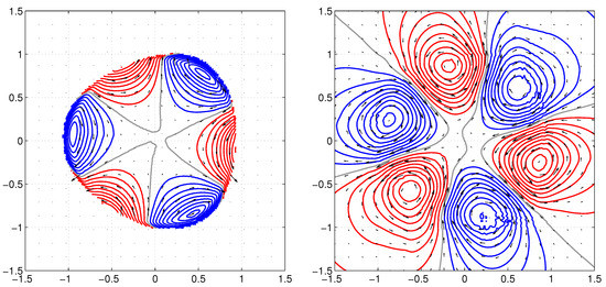
Figure 6.
Upper (left) and lower (right) non-axisymmetric parts of the pressure (lines) and velocity (arrows) at for the simulation initialized with a perturbation in the upper layer. Positive values of the pressure perturbation are in blue and negative values are in red.
The standard picture of a frontal mode in the upper layer and Rossby mode in the lower layer (with the velocity along the pressure isolines) clearly emerges, and matches the structure of the linear unstable mode (not shown, but one can compare with Gula and Zeitlin [39] in the rotating annulus): the growing perturbation manifests itself by the non-axisymmetric shape of the vortex in the left panel.
3.4. Sensitivity to the Initial Conditions
When initially perturbed with several wavenumbers, several unstable modes with differ‘ent wavenumbers may develop, as might be expected from the linear stability analysis. This is visible in Figure 7 (left panel), where the evolution of the modal amplitude of the perturbation in one numerical run is plotted and exhibits linear growth for two wavenumbers. It is different from what is observed in the laboratory experiments, where a single wavenumber most often emerges. We suspected this could be due to the difference in the initial perturbation. We thus consider the destabilization of the eddy with and discussed previously, in five nonlinear simulations using 3 different types of initial perturbation. The first consists of a random noise with different azimuthal wavenumbers; the second consists of noise with the same radial structure as before but only one wavenumber (we consider and ); the last one consists of the linearly unstable mode, as shown previously (two runs). The basic vortex profile is linearly unstable with respect to wavenumbers 2 and 3, and the associated growth rates are and , respectively. In the nonlinear simulations, we find growth rates of and for and , respectively, both in the simulation initialized with several wavenumbers and with a single wavenumber, as shown in Figure 7.
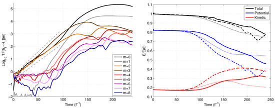
Figure 7.
(Left): Evolution of the upper layer thickness perturbation (logarithm of norm) for different wavenumbers for the simulation with initial conditions randomly perturbed (several wavenumbers). Dashed lines indicate the estimated growth rate ( for and for ). (Right): Evolution of the energy anomaly (total: black, potential: blue, kinetic: red) normalized by the initial total energy anomaly. Thick continuous lines: perturbation containing a range of wavenumbers, thick dashed lines: perturbation with , thin continuous lines: perturbation with . Vortex parameters: , .
The development of this instability is associated with a transfer from potential to kinetic energy. The evolution of the relative energy anomaly, with the potential energy on the same domain with the lens subtracted, is shown in Figure 7 (right panel) for the three different runs with different initial perturbation (multiple wavenumbers, and ). The energy transfer starts at the initial instant, as seen from the slight but constant decrease in potential energy. However, there is no visible increase in the kinetic energy at this time, probably due to dissipation. Nonlinear saturation, as seen in the decrease of the linear growth rate (cf. Figure 7), occurs around here and is associated with an enhancement of the energy transfer, which stops later on (at about depending on the simulation). During the same time, the dipoles form and start moving away from the initial vortex position. For the m = 2 instability, corresponds to when the vortex becomes pinched near its center, while it is associated with the arms beginning to roll up for the m = 3 instability. Rather surprisingly, the development of the instability, as seen in the evolution of the energy, is actually slower for the simulation perturbed with several wavenumbers compared to the m = 2 perturbation alone associated with the strongest transfer. To our knowledge, this kind of sensitivity to the initial perturbations has not been reported before.
4. Nonlinear Saturation of the Instability
We now turn to the mature stage and nonlinear saturation of the instability, relying mostly on nonlinear numerical simulations and comparing with laboratory experiments when appropriate. The range of parameters investigated in the former is the same as in the latter (see Table 1). In addition, we performed a set of simulations with and already discussed in the previous section. The latter serves as a reference for the discussion of the nonlinear saturation of the instability, and is presented in detail. The outcome of the nonlinear saturation of the instability is not unique: it may be divided into 3 different scenarios, depending on whether the dominant unstable mode consists of (1) one wavenumber , (2) one wavenumber , or (3) a superposition of several wavenumbers. For the same initial vortex, one of the above situation can be picked by choosing the proper initial perturbation, provided the vortex is unstable with respect to several wavenumbers with nearby growth rates. This is particularly true (see previous section) for the vortex with , described below.
4.1. Nonlinear Saturation for Dominant
The destabilization of the vortex in this case is similar to the standard “dipolar vortex breaking” observed as the outcome of barotropic instability (e.g., [29,30], and references therein). Developing arms start rolling up in a cyclonic sense (although the circulation within the arms is anticyclonic) and form a dipole with a lower-layer cyclonic circulation associated with the positive PV anomaly shredding from the initial core. The destabilized vortex is shown in Figure 8 (first row) at two different stages, and the corresponding lower-layer PV is shown in Figure 9 below. The lower layer is nearly balanced (in the geostrophic sense) and circulation may thus be inferred from the pressure gradient. The self-mutual interaction of the poles is baroclinic, as each pole is in a different layer, and is more heton-like [29,42]. As the dipoles radiate away, they detach and eventually leave a monopole at the location of the initial vortex, which looks like an elliptical “cat’s eye” vortex. In some case, weaker satellites result from the filaments between the radiating dipole and the monopole (on the right above the monopole and below it on the left in Figure 8, upper-right panel). The magnitude of this monopole is larger for larger values of , and is almost negligible for small values (within the parameter range investigated in our numerical simulations and leading to a wavenumber 2 unstable mode). It is worth mentioning that the radial momentum of the dipoles almost vanishes once they detach from central monopole. Almost all of the lower-layer initial patch of PV splits off and moves along with the baroclinic dipoles, or is stirred during of the detachment of the latter, so that the PV anomaly under the remaining elliptical monopole is very weak, enhancing its stability (see Section 5.2 for a discussion of the impact of a vanishing lower-layer PV gradient). This concludes the nonlinear saturation of the instability, as a marginally stable state is thus reached. The situation shown at in Figure 8 (upper row, right panel) is quite representative of a quasi-stationary state observed until the end of the simulation at .


Figure 8.
Snapshots of thickness (grey shading, black for ) and pressure in the upper layer (black contour at intervals of starting from 0) and lower layer (positive in blue, negative in red, at intervals of ) for the simulations initialized with perturbation (first row), perturbation (second row) and several wavenumbers (last row) at (left column) ant (right panel), corresponding roughly to 5 and 10 inverse growth rate. Initial vortex profile parameters: , .
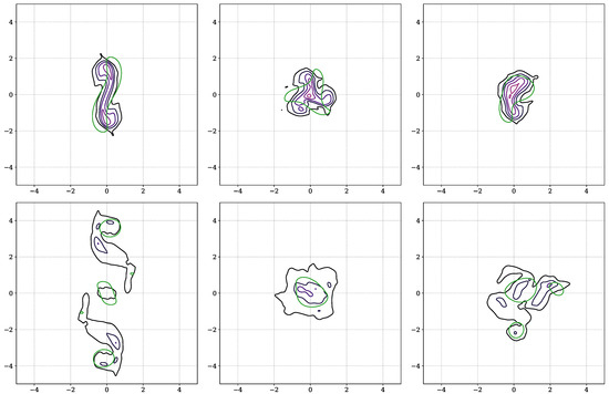
Figure 9.
Evolution of the lower-layer PV at (upper row) and (lower row), for the eddy with and initialised with azimuthal mode number (left column), (middle column) or several wavenumbers (right column); corresponding to the pressure and layer thickness shown in Figure 8 (panels are transposed). The nondimensional lower-layer PV anomaly is contoured every from black to purple, starting at . The green contour indicates upper layer thickness at value .
4.2. Nonlinear Saturation with Wavenumber(s)
Cyclonic arms also develop for vortices that are unstable with respect to one or several mode number(s) larger than 2. However, they hardly ever detach from the initial vortex nor propagate away from it. Rather, as can be seen in the second and last row of Figure 8, the baroclinic dipoles formed rotate on their own and stay in the same neighbourhood. At later times, they adjust toward monopoles (as in Figure 8), or eventually remerge with the main anticyclone.
It is interesting to note the differences between the development and outcome of the destabilization when several wavenumbers develop simultaneously. In particular, the arms often detach at different times. In the case given in Figure 8, at , only one dipole in the process of forming is visible, whereas there are as many as the wavenumber of the initial perturbation in the two upper rows. At , one can see that another dipole has detached (to the right of the main anticyclone) and additional, much weaker patches are visible, e.g., to the left of the main anticyclone. Again, this is representative of many cases.
The saturation of the instability in the numerics is quantitatively different from what is observed in the laboratory experiments. In the latter, the initial vortex is always completely destroyed (meaning that all the lighter fluid initially in the eddy went into the dipoles), while we do observe a remaining (somewhat weak) monopole at the initial location of the eddy in the numerics. This sheds light on the uncertainties associated with both numerical and laboratory experiment, and especially on the initialization of the flow, as discussed throughout the paper.
Although a detailed comparison of the different models is beyond the scope of this manuscript, the scenario of the breakup of the vortex is qualitatively similar to non-outcropping QG or RSW vortices with in either a gaussian shape or a piecewise-constant PV distribution (e.g., [24,31,40]).
5. Discussion: Impact of a Lower-Layer Flow
To date, in our nonlinear numerical simulations and linear stability analysis, we have only considered basic states with the lower layer at rest. In this case, the lower-layer PV is given by , and its radial variation allows for the propagation of a Rossby wave that can resonate a upper-layer wave to give rise to an instability. This is highlighted in Figure 9 which shows the evolution of the lower PV (Note that, due to discretisation errors in the vicinity of the outcropping region, PV is not exactly conserved and develops small sharp perturbations, including in the lower layer. For visualization purpose, we smoothed the computed PV field using a Gaussian kernel of width equal to 4 grid cells.) during the development of the instability for the vortex with , previously shown in Figure 8. The role of the lower-layer PV in the instability is obvious from its phase quadrature with the upper layer at early stages of the instability (best visible in simulations initialized with well-defined azimuthal mode number—see the left and center upper panels), typical of baroclinic instability.
However, the actual inviscid solutions associated with the experimental configuration we used are different. In particular, the lower-layer PV has a piecewise-constant radial profile, as shown in Figure 10. It is also different in the other standard experimental method for producing lenticular vortices, the “constant-flux” experiment [16]. In the latter configuration, where fluid is gradually injected from a small source at the surface, conservation of the lower-layer PV implies that its value is constant and the same as the planetary PV outside the eddy. While fluid is being injected, fluid parcels in the lower layer are pushed radially outward and thereby acquire negative relative velocity. As a result, the lower layer is co-rotating with the upper layer (cf. Figure 10, lower right panel, orange line). (An approximate analytic solution for this configuration, neglecting the centrifugal term in the lower layer, was derived by Griffiths and Linden [16].) On the contrary, as discussed in Section 2.1, a weak counter-rotating circulation forms in the constant-volume experiment.
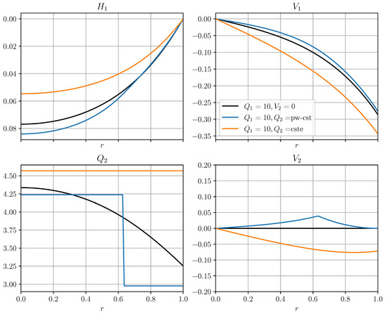
Figure 10.
Vortex profiles (same fields as Figure 1) with different lower-layer conditions: quiescent (; black), piecewise-constant PV (blue) and constant PV (orange). Vortex parameters: , .
A solution with a constant lower-layer PV is a plausible configuration for realistic ocean eddies. Indeed, deep ocean flows are weaker than surface currents and thereby associated with very weak departure of the PV from the background planetary vorticity. Thus, as an eddy propagates above this quiescent deep layer, it will slightly moves the isopycnal down which will implies the development of a weak co-rotating flow in the deep layer, through PV conservation. Although very qualitative, this is somewhat in agreement with the deep extension of eddies reported from various observations (e.g., [2,8,9]). Based on this remark, one can argue that constant-PV lower layer is at least as plausible as a lower-layer at rest.
One would expect that the vanishing of the PV gradient and the associated suppression of Rossby waves would remove the instability, as was shown for nonisolated eddies [25,43] and more recently for warm-core eddies in the RSW model [26]. We thus consider lenticular vortices with profiles corresponding to the two situations mentioned, which are shown in Figure 10.
5.1. Piecewise-Constant Lower-Layer PV
The jump in at yields a cusp in the velocity profile, as follows from Equation (5) (see Figure 10 around ). As spectral methods do not cope well with discontinuities, we smooth the profile of (and, correspondingly, the cusp in ) using a third-order polynomial that matches both the values of and its derivative (which is zero) at for the numerical resolution of the linear eigenproblem. The linear stability calculation is performed over a restricted range of values for : and .
The instability regime we found with this configuration is marginally changed by the lower layer flow compared to the quiescent lower layer. Therefore, it is not shown here, and we refer the reader to Figure 3. The most striking difference is that the growth rate of the instability vanishes for (). For , the growth rate is very similar for low values of , which is not surprising as the lower-layer flow remains weak. For larger values of the depth ratio (), the growth rate for piecewise-constant is lower than that for , the more so as increases. We found weakly unstable modes. ( for ) for , which have critical levels associated with the lower layer flow. However, their physical relevance is unclear and the basic flow in this region tends to be unrealistic, as the lower layer velocity peaks at values similar (in absolute value) to the upper layer flow and the initial value of the depth ratio (before the adjustment) is very high: in particular, neglecting viscous effects in the lower layer is not appropriate in this configuration.
We also tried running four nonlinear simulation initialized with this modified vortex profile for and , and and 25. These simulations did not exhibit significant difference compared to their counterpart with , confirming the previous results from the linear stability analysis.
5.2. Constant Lower-Layer PV
The equations for the background state are unchanged, except that the lower layer PV is now , and the boundary condition for the lower-layer velocity is different: . The only solution that reproduces the inviscid “constant flux” experiment adjusted state has , which is associated with solid-body rotation (e.g., [16]). We investigated, however, a broader range of values for , considering that eddies produced in oceanic flows, e.g., by detaching from boundary currents, can have non-zero PV values.
From the linear stability analysis, we found no unstable mode in the range of parameters investigated: and , except for the highest values of and low values of where the frontal-frontal instability occurs (not shown, but see Figure 3, lower right corner). This result is in agreement with the fact that the absence of gradient of PV in the lower layer prevents the propagation of a Rossby mode, thus suppressing the instability resulting from its resonance with the upper-layer modes. This also confirms some results previously reported in the literature [24,25,26]. It is worth mentioning that we still found ageostrophic instability for very high values of and wavenumbers , which was not reported in Cohen et al. [26] as they did not investigate the corresponding range of parameters (note that is unrealistic in oceanic flows, except over shallow regions such as continental shelves).
We verified the inhibition of the instability by the constant lower PV was verified by means of nonlinear simulations for two sets of parameters: , and , (not shown). The typical dimensional parameters of the first eddy were already given above, and the second case corresponds to a fairly large (Bu ∼ 0.03) and intense (Ro ∼ 0.3) vortex. These simulations shown that the vortices eventually destabilized, but only after a significant part of the lower layer velocity sustaining the constant PV dissipated, thereby restoring a PV anomaly in the lower layer. Once a significant lower-layer PV was reached (around half the magnitude of the lower PV in the quiescent lower layer configuration), the eddy started destabilizing, with a typical timescale that was clearly extended (by at least a factor 2) compared to the simulations with . These results tend to confirm the stabilization of the vortex by the constant lower-layer PV.
To obtain more insight about the impact of the lower-layer flow, we investigate the linear stability of profiles that lie in between the two extreme configurations for the lower layer: (1) no flow (); and (2) constant PV (). We consider a class of solutions with with the lower layer velocity proportional to the constant-PV solution with a factor (as in, [43]). The layer thickness are recomputed afterwards by solving (7), with held constant. Note that the value of , and hence the dimensional size of the vortex , vary with . (Other “paths” for the evolution of the vortex profile can be used, e.g., by keeping the dimensional volume of the lens of fluid constant, which would probably be a better approximation to experimental flows. However, we do not aim at modelling precisely the evolution of the eddy under bottom friction.) The evolution of the growth rate as a function of is given in Figure 11 for two different values of . One sees that the growth rate of all the unstable modes vanishes continuously as the lower layer flow evolves towards a zero PV-gradient solution.
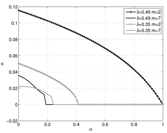
Figure 11.
Evolution of the growth rate of the most unstable mode, , as the lower-layer flow evolves from the rest-state to the zero PV anomaly solution, for a lenticular vortex with zero PV in the upper layer. Vortex depth ratios , and azimuthal wave numbers , 7. No other unstable mode was found.
6. Conclusions
In this study, we investigated the instability of constant-PV warm-core eddies in a two-layer Rotating Shallow Water model, by means of a linear stability analysis, laboratory experiments and nonlinear numerical simulations. We now summarize the results of this work.
A linear stability analysis was first carried and a stability diagram was constructed. It shows the dependence of the growth rate and wavenumber of the most unstable mode with respect to the depth ratio of the eddy and the value of the upper Potential Vorticity (PV), for an eddy over a quiescent lower layer and with the rigid-lid approximation. We confirmed the following results, previously reported in the litterature ([19,23], and references therein):
- The instability domain is dominated by the hybrid instability, associated with resonance between a frontal mode and a lower-layer Rossby wave.
- The growth rate of the most unstable mode increases with the depth ratio and slightly decreases (increases) with the value of the PV of the eddy for small (large) values of the depth ratio. The wavenumber of the most unstable mode increases with both depth ratio and the eddy PV. Several unstable modes with close growth rates and wavenumbers co-exist for .
We also reported some results that were not discussed in former studies, to our knowledge:
- Some unstable modes may be found in the zone of stability in the lower-left corner of the parameter space.
- For very large aspect ratio, we found a very unstable ageostrophic unstable mode with high wavenumber (), associated with the resonance between Poincare-like waves.
Moving to a linear stability analysis, we then investigated the impact of the lower flow:
- If the lower-layer PV is constant (relevant for oceanic application and “constant-flux” experiments, and associated with a weak co-rotating lower-layer circulation), the hybrid instability vanishes as no lower-layer PV gradient supporting the Rossby wave propagation is present. As a result, the vortex is found to be stable, as was previously suggested (e.g., [24,25]) and confirmed by a linear stability analysis in the same model by Cohen et al. [26] with a different numerical method. We further confirmed this inhibition of the instability by means of nonlinear numerical simulations. The ageostrophic instability for very high depth ratio persists (from the linear stability analysis), which was not previously reported.
- If the lower layer is piecewise-constant (corresponding to the inviscid adjusted state in “constant-volume” laboratory experiments and associated with a weak counter-rotating lower-layer circulation), the stability properties are hardly changed for , as shown by both the linear stability analysis and the nonlinear simulations. The growth rate is slightly lower for large depth ratio. For , no significant unstable mode has been found, but weakly unstable mode may exist for high values of the depth ratio.
The destabilization of the vortex was studied by means of “constant-volume” laboratory experiments (release of lighter fluid initially contained in a cylinder at the center of a rotating tank filled with denser fluid) and numerically using a high-resolution finite-volume scheme of the two-layer RSW equations. For a wide range of vortex parameters, the wavenumber of the unstable mode observed in the laboratory experiments, as well as the growth rate measured in the numerical simulations, showed good agreement with the linear theory prediction. However, from a more quantitative point of view, some discrepancies were observed:
- The wavenumber observed in laboratory experiments was sometimes different than the linear prediction, especially for large values of the depth ratio;
- The growth rate in the numerical experiments is lower that expected from the linear stability analysis (between 10% and 40%, increasing with ).
These differences could be caused by friction effects: the Ekman damping in the lower layer (laboratory experiments) becomes important for large values of , while friction near the edge of the eddy can have an impact, especially for large where the velocity profile peaks at the edge. More importantly, we observed that the wavenumber of the developing unstable mode is sensitive to the initial perturbation. In the numerical simulations, while single-valued high azimuthal wavenumber perturbation is not enough to trigger instability, a superposition of several wavenumbers leads to the concurrent development of several unstable modes (if present). On the other hand, instability seems to be fed by high-wavenumber perturbation in the laboratory experiments although, in most cases, it exhibits a single well-defined wavenumber at mature stage.
The nonlinear saturation of the instability, afterwards the initial development of (typically m) arms rolling-up in a cyclonic sense, can be classified as follows:
- for , two baroclinic dipoles form and propagate away from the initial eddy, leaving eventually a weak monopole at the center;
- for , several dipoles propagate with a strongly curved direction. As a result, they sometimes stay in the neighbourhood of the initial eddy, interacting in a complex manner with each other. Again, a weak monopole can be left at the location of the initial location of the eddy, depending on the parameters.
Here again, differences are observed between the numerical simulations and the laboratory experiments. In particular, the destabilization of the vortex in the numerical simulations appears more chaotic when several unstable modes (with different wavenumbers) develop, as they nonlinearly interact with each other. Moreover, it is very rare to observe a leftover monopole at the center of the domain in the laboratory experiments, as almost all the initial lighter fluid moved away inside the baroclinic dipoles. Although it is difficult to identify the origin of these discrepancies, one should bear in mind that dynamical parameters of the eddies produced in the laboratory experiment are estimated from simple heuristic arguments. As a result, for instance, the spectra of unstable modes associated with the actual eddy produced could be different resulting in one mode being dominant over the others, which would lead to a “simpler“development of the instability as observed.
The results presented in this paper strengthen the need to investigate the impact of the environment of eddies to better understand their instability properties. In particular, we found that the lower-layer flow may act to suppress the instability. In this direction, investigating the role of smaller-scale turbulence (e.g., random fluctuations in the lower layer) could provide very interesting information regarding the stability of ocean eddies.
Author Contributions
Conceptualization, methodology, formal analysis: all three authors. Investigation and visualization: N.L. and A.P.; Data curation: A.P. and N.L.; writing—original draft preparation, N.L.; writing—review and Editing: A.P. and S.G.L.S.; supervision, project administration and funding acquisition, S.G.L.S. All authors have read and agreed to the published version of the manuscript.
Funding
The laboratory experiments and linear analysis were carried out during A. Paci’s internship funded by METEO-FRANCE and S.G.L.S. at UCSD under the supervision of S.G.L.S. and Paul Linden. The numerical simulations were carried out during N. Lahaye postdoc supported by ONR Award N00014-13-1-0347, under the supervision of S.G.L.S.
Institutional Review Board Statement
Not applicable.
Informed Consent Statement
Not applicable.
Data Availability Statement
Numerical codes used to produce the results are available upon request.
Acknowledgments
We are grateful to three anonymous reviewers for providing useful suggestions that helped improving the quality of this manuscript. Paul Linden is acknowledged for their involvement in the beginning of the work (especially during A. Paci’s internship), and further useful discussions.
Conflicts of Interest
The authors declare no conflict of interest. The funders had no role in the design of the study; in the collection, analyses, or interpretation of data; in the writing of the manuscript, or in the decision to publish the results.
Abbreviations
The following abbreviations are used in this manuscript:
| PV | Potential Vorticity |
| RSW | Rotating Shallow Water |
| QG | Quasi-Geostrophic |
Appendix A. Linear Problem in the Exterior Domain (r > 1) and Boundary Conditions
In the exterior problem, the vertical configuration simplifies to a single active layer. The rigid-lid assumption and constant-PV condition require the basic state velocity to decrease as (the associated relative vorticity must be zero). The linearized equations for and p (omitting the layer index) thus become:
where we have introduced the intrinsic frequency . Since , the following relation holds:
Cancelling the pressure terms between (A1) and (A2), using the above equality and (A3), leads to the constraint
This relation states that the vorticity of any normal mode vanishes in the exterior region, except at critical levels where . However, this does not concern unstable modes for which . From (A3), we can express the velocities using a stream function :
Hence, upon insertion of this form in (A4), the streamfunction satisfies a Laplace equation with the condition as . This gives the following relation:
which is used as a boundary condition at to ensure continuity of the eigenfunction across . Finally, (A1) and (A2) can be combined to express u and v as functions of p and its first derivative:
Using , these equations yield a relation between p and its first radial derivative which provides the inhomogeneous linear boundary condition (14), again by imposing continuity of p and at .
Appendix B. Initial Conditions for the Nonlinear Numerical Simulations
The initial conditions consist of the inviscid solution slightly perturbed by applying a map on the radial variable, i.e.,
The simplest function , which is the one we consider here, does not depend on r and consists of a superposition of azimuthal modes:
where is a random phase and a random amplitude picked up from a Gaussian distribution with mean value and standard deviation . The resulting thickness and velocity field are thus nearly balanced and the boundary of the vortex is at . However, the angular derivative of the azimuthal velocity is no longer zero because of the axisymmetry. We thus add a perturbation to the radial velocity to ensure that the divergence is nearly zero:
The lower layer thickness is such that the pressure in the lower layer is unperturbed (hence the lower layer remains strictly balanced): .
Appendix C. Linear Stability Analysis with a Free Surface
We carried out the linear calculations presented in Section 3.1 with the free surface configuration, and give a rapid description of the features that differ from the rigid-lid configuration here.
While the solution for the basic vortex is hardly changed (the only modification is that ), there is no longer a boundary condition at . For a quiescent exterior fluid, the solution is given analytically by Bessel functions, which do not provide boundary conditions at that are linear in the eigenvalue. Hence, the linear problem is supplemented by the lower-layer equations in the semi-infinite outer domain (), which is solved using rational polynomials obtained by an algebraic mapping of the standard Chebyshev series [30,44]. Continuity of and at was ensured.
The corresponding spectrum of unstable modes was show in comparison with results from the nonlinear numerical simulations in Figure 5, right label (only a portion of the domain was shown). The relative difference between the free-surface and rigid-lid, for a value of the density ratio of , is less that 10% for and of the order of 15% for lower . This error associated with the rigid lid approximation increases with and decreases with . The only remarkable emerging features are frontal-frontal modes (e.g., [19]) that manifest themselves emerging from the bottom of the figure for very deep eddies (around ).
Appendix D. Laboratory Experiments Parameters
Table A1.
Parameters of the laboratory experiments: experimental configuration are in the first 7 columns, estimated nondimensional parameters of the adjusted vortex in the next 4 columns, and observed most unstable mode number in last column. Symbols are explained in the text. Bold values are for the experiment shown in Figure 4.
| m | |||||||||||
|---|---|---|---|---|---|---|---|---|---|---|---|
| cm/s | cm | cm | cm | rad/s | |||||||
| 0.330 | 0.110 | 5.0 | 5.5 | 40.0 | 4.5 | 0.75 | 8.66 | 0.10 | 7.5 | 0.12 | 2 |
| 0.160 | 0.095 | 5.0 | 5.5 | 40.0 | 3.8 | 1.00 | 7.70 | 0.09 | 12.3 | 0.08 | 2 |
| 0.880 | 0.175 | 3.8 | 5.5 | 40.0 | 7.0 | 0.50 | 10.66 | 0.14 | 4.3 | 0.18 | 2 |
| 0.280 | 0.150 | 3.8 | 5.5 | 40.0 | 6.0 | 0.83 | 8.41 | 0.14 | 8.4 | 0.11 | 2 |
| 0.190 | 0.150 | 3.8 | 5.5 | 40.0 | 6.0 | 1.00 | 7.90 | 0.14 | 10.9 | 0.09 | 2 |
| 0.120 | 0.150 | 3.8 | 5.5 | 40.0 | 6.0 | 1.25 | 7.41 | 0.15 | 15.1 | 0.07 | 2 |
| 0.230 | 0.100 | 6.9 | 5.5 | 40.0 | 4.0 | 1.00 | 8.14 | 0.10 | 9.5 | 0.10 | 2 |
| 0.144 | 0.100 | 6.8 | 5.5 | 40.0 | 4.0 | 1.25 | 7.59 | 0.10 | 13.2 | 0.07 | 2 |
| 0.260 | 0.195 | 4.4 | 5.5 | 20.5 | 4.0 | 0.75 | 8.30 | 0.18 | 8.8 | 0.10 | 2 |
| 0.093 | 0.195 | 4.4 | 5.5 | 20.5 | 4.0 | 1.25 | 7.18 | 0.19 | 18.3 | 0.05 | 3 |
| 0.146 | 0.195 | 4.4 | 5.5 | 20.5 | 4.0 | 1.00 | 7.60 | 0.19 | 13.1 | 0.07 | 2 |
| 0.420 | 0.400 | 3.2 | 5.5 | 10.0 | 4.0 | 0.50 | 9.06 | 0.35 | 6.5 | 0.13 | 2 |
| 0.185 | 0.400 | 3.2 | 5.5 | 10.0 | 4.0 | 0.75 | 7.87 | 0.38 | 11.1 | 0.09 | 2 |
| 0.067 | 0.400 | 3.2 | 5.5 | 10.0 | 4.0 | 1.25 | 6.92 | 0.39 | 23.7 | 0.04 | 4 |
| 0.086 | 0.400 | 3.2 | 5.5 | 10.0 | 4.0 | 1.10 | 7.11 | 0.39 | 19.4 | 0.05 | 4 |
| 0.066 | 0.630 | 2.5 | 5.5 | 8.0 | 5.0 | 1.25 | 6.91 | 0.62 | 23.9 | 0.04 | 4 |
| 0.460 | 0.560 | 6.3 | 5.5 | 9.0 | 5.0 | 0.75 | 9.23 | 0.49 | 6.1 | 0.14 | 2 |
| 0.170 | 0.630 | 6.3 | 5.5 | 8.0 | 5.0 | 1.25 | 7.77 | 0.60 | 11.7 | 0.08 | 4 |
| 0.100 | 0.088 | 6.3 | 5.5 | 40.0 | 3.5 | 1.35 | 7.24 | 0.09 | 17.3 | 0.06 | 2 |
| 0.055 | 0.175 | 17.6 | 20.0 | 28.5 | 28.5 | 1.00 | 24.69 | 0.17 | 27.7 | 0.04 | 4 |
| 0.037 | 0.175 | 11.9 | 20.0 | 28.5 | 28.5 | 1.00 | 23.85 | 0.17 | 38.4 | 0.03 | 5 |
| 0.023 | 0.175 | 7.4 | 20.0 | 28.5 | 28.5 | 1.00 | 23.03 | 0.17 | 57.7 | 0.02 | 6 |
| 0.088 | 0.193 | 25.8 | 20.0 | 28.5 | 28.5 | 1.00 | 25.93 | 0.19 | 19.1 | 0.05 | 3 |
| 0.135 | 0.175 | 43.4 | 20.0 | 28.5 | 28.5 | 1.00 | 27.35 | 0.17 | 13.9 | 0.07 | 3 |
| 0.015 | 0.175 | 6.8 | 20.0 | 28.5 | 28.5 | 1.00 | 22.45 | 0.17 | 84.0 | 0.02 | 7 |
| 0.196 | 0.190 | 36.5 | 20.0 | 28.7 | 28.7 | 1.20 | 28.85 | 0.18 | 10.6 | 0.04 | 3 |
| 0.046 | 0.100 | 18.5 | 20.0 | 39.5 | 39.5 | 0.80 | 24.29 | 0.10 | 32.1 | 0.05 | 3 |
| 0.030 | 0.100 | 17.1 | 20.0 | 39.5 | 39.5 | 1.00 | 23.46 | 0.10 | 45.9 | 0.03 | 4 |
| 0.022 | 0.100 | 11.0 | 20.0 | 39.5 | 39.5 | 1.20 | 22.97 | 0.10 | 59.9 | 0.01 | 5 |
| 0.056 | 0.100 | 28.7 | 20.0 | 39.0 | 39.0 | 1.20 | 24.73 | 0.10 | 27.3 | 0.03 | 3 |
| 0.018 | 0.100 | 10.5 | 20.0 | 39.0 | 39.0 | 1.20 | 22.68 | 0.10 | 71.5 | 0.01 | 5 |
| 0.200 | 0.600 | 53.7 | 20.0 | 10.0 | 6.0 | 1.00 | 28.94 | 0.56 | 10.5 | 0.09 | 3 |
| 0.100 | 0.670 | 25.9 | 20.0 | 10.5 | 7.0 | 1.00 | 26.32 | 0.65 | 17.3 | 0.06 | 4 |
| 0.062 | 0.600 | 16.4 | 20.0 | 10.0 | 6.0 | 1.00 | 24.98 | 0.59 | 25.2 | 0.04 | 5 |
| 0.041 | 0.600 | 11.0 | 20.0 | 10.0 | 6.0 | 1.00 | 24.05 | 0.58 | 35.3 | 0.03 | 6 |
| 0.055 | 0.600 | 14.8 | 20.0 | 10.0 | 6.0 | 1.00 | 24.69 | 0.59 | 27.7 | 0.04 | 5 |
| 0.052 | 0.600 | 13.9 | 20.0 | 10.0 | 6.0 | 1.00 | 24.56 | 0.59 | 29.0 | 0.03 | 5 |
| 0.025 | 0.400 | 9.8 | 20.0 | 10.0 | 4.0 | 1.00 | 23.16 | 0.40 | 53.6 | 0.02 | 7 |
| 0.030 | 0.400 | 12.0 | 20.0 | 10.0 | 4.0 | 1.00 | 23.46 | 0.40 | 45.9 | 0.02 | 5 |
| 0.031 | 0.194 | 8.4 | 20.0 | 31.0 | 6.0 | 1.00 | 23.52 | 0.19 | 44.6 | 0.02 | 5 |
| 0.037 | 0.194 | 9.8 | 20.0 | 31.0 | 6.0 | 1.00 | 23.85 | 0.19 | 38.4 | 0.03 | 5 |
| 0.026 | 0.194 | 6.9 | 20.0 | 31.0 | 6.0 | 1.00 | 23.22 | 0.19 | 51.9 | 0.02 | 5 |
References
- McWilliams, J.C. Submesoscale, coherent vortices in the ocean. Rev. Geophys. 1985, 23, 165–182. [Google Scholar] [CrossRef]
- Olson, D.B. Rings in the Ocean. Annu. Rev. Earth Planet. Sci. 1991, 19, 283–311. [Google Scholar] [CrossRef]
- Carton, X. Oceanic vortices. In Fronts, Waves and Vortices in Geophysical Flows; Flòr, J., Ed.; Springer: Berlin/Heidelberg, Germany, 2010; Volume 805, pp. 61–108. [Google Scholar]
- Chelton, D.; Schlax, M.; Samelson, R. Global observations of nonlinear mesoscale eddies. Progr. Oceanogr. 2011, 91, 167–216. [Google Scholar] [CrossRef]
- Paci, A.; Caniaux, G.; Gavart, M.; Giordani, H.; Lévy, M.; Prieur, L.; Reverdin, G. A High-Resolution Simulation of the Ocean during the POMME Experiment: Simulation Results and Comparison with Observations. J. Geophys. Res. Ocean. 2005, 110. [Google Scholar] [CrossRef]
- Paci, A.; Caniaux, G.; Giordani, H.; Lévy, M.; Prieur, L.; Reverdin, G. A High-Resolution Simulation of the Ocean during the POMME Experiment: Mesoscale Variability and near Surface Processes. J. Geophys. Res. Ocean. 2007, 112. [Google Scholar] [CrossRef]
- Flierl, G.R. A simple model for the structure of warm and cold core rings. J. Geophys. Res. Ocean. 1979, 84, 781–785. [Google Scholar] [CrossRef]
- de Marez, C.; L’Hégaret, P.; Morvan, M.; Carton, X. On the 3D Structure of Eddies in the Arabian Sea. Deep Sea Res. Part I Oceanogr. Res. Pap. 2019, 150, 103057. [Google Scholar] [CrossRef]
- Olson, D.B. The Physical Oceanography of Two Rings Observed by the Cyclonic Ring Experiment. Part II: Dynamics. J. Phys. Oceanogr. 1980, 10, 514–528. [Google Scholar] [CrossRef]
- Olson, D.B.; Evans, R.H. Rings of the Agulhas Current. Deep Sea Res. Part A Oceanogr. Res. Pap. 1986, 33, 27–42. [Google Scholar] [CrossRef]
- Goni, G.J.; Garzoli, S.L.; Roubicek, A.J.; Olson, D.B.; Brown, O.B. Agulhas Ring Dynamics from TOPEX/POSEIDON Satellite Altimeter Data. J. Mar. Res. 1997, 55, 861–883. [Google Scholar] [CrossRef][Green Version]
- Petersen, M.R.; Williams, S.J.; Maltrud, M.E.; Hecht, M.W.; Hamann, B. A Three-Dimensional Eddy Census of a High-Resolution Global Ocean Simulation. J. Geophys. Res. Ocean. 2013, 118, 1759–1774. [Google Scholar] [CrossRef]
- McWilliams, J.C. A Survey of Submesoscale Currents. Geosci. Lett. 2019, 6, 3. [Google Scholar] [CrossRef]
- Saunders, P.M. The Instability of a Baroclinic Vortex. J. Phys. Oceanogr. 1973, 3, 61–65. [Google Scholar] [CrossRef]
- Gill, A.; Smith, J.; Cleaver, R.; Hide, R.; Jonas, P. The vortex created by mass transfer between layers of a rotating fluid. Geophys. Astrophys. Fluid Dyn. 1979, 12, 195–220. [Google Scholar] [CrossRef]
- Griffiths, R.W.; Linden, P.F. The stability of vortices in a rotating, stratified fluid. J. Fluid Mech. 1981, 105, 283–316. [Google Scholar] [CrossRef]
- Flierl, G.R. Rossby Wave Radiation from a Strongly Nonlinear Warm Eddy. J. Phys. Oceanogr. 1984, 14, 47–58. [Google Scholar] [CrossRef]
- Gula, J.; Zeitlin, V.; Bouchut, F. Instabilities of Buoyancy-Driven Coastal Currents and Their Nonlinear Evolution in the Two-Layer Rotating Shallow Water Model. Part 2. Active Lower Layer. J. Fluid Mech. 2010, 665, 209–237. [Google Scholar] [CrossRef]
- Ribstein, B.; Zeitlin, V. Instabilities of Coupled Density Fronts and Their Nonlinear Evolution in the Two-Layer Rotating Shallow-Water Model: Influence of the Lower Layer and of the Topography. J. Fluid Mech. 2013, 716, 528–565. [Google Scholar] [CrossRef]
- Boss, E.; Paldor, N.; Thompson, L. Stability of a Potential Vorticity Front: From Quasi-Geostrophy to Shallow Water. J. Fluid Mech. 1996, 315, 65–84. [Google Scholar] [CrossRef][Green Version]
- Ripa, P. Instability of a solid-body rotating vortex in a two-layer model. J. Fluid Mech. 1992, 242, 395–417. [Google Scholar] [CrossRef]
- Paldor, N.; Nof, D. Linear instability of an anticyclonic vortex in a two-layer ocean. J. Geophys. Res. 1990, 95, 18075–18079. [Google Scholar] [CrossRef]
- Cohen, Y.; Dvorkin, Y.; Paldor, N. Linear instability of warm core, constant potential vorticity, eddies in a two-layer ocean. Q. J. R. Meteorol. Soc. 2015, 141, 1884–1893. [Google Scholar] [CrossRef]
- Dewar, W.K.; Killworth, P.D. On the stability of oceanic rings. J. Phys. Oceanogr. 1995, 25, 1467–1487. [Google Scholar] [CrossRef]
- Benilov, E.S. Stability of vortices in a two-layer ocean with uniform potential vorticity in the lower layer. J. Fluid Mech. 2004, 502, 207–232. [Google Scholar] [CrossRef]
- Cohen, Y.; Dvorkin, Y.; Paldor, N. On the stability of outcropping eddies in a constant PV ocean. Q. J. R. Meteorol. Soc. 2016, 142, 1920–1928. [Google Scholar] [CrossRef]
- Ikeda, M. Instability and splitting of mesoscale rings using a two-layer quasi-geostrophic model on a f-plane. J. Phys. Oceanogr. 1981, 11, 987–998. [Google Scholar] [CrossRef]
- Gent, P.R.; McWilliams, J.C. The instability of barotropic circular vortices. Geophys. Astrophys. Fluid Dyn. 1986, 24, 209–233. [Google Scholar] [CrossRef]
- Baey, J.M.; Carton, X. Vortex multipoles in two-layer rotating shallow-water flows. J. Fluid Mech. 2002, 460, 151–1753. [Google Scholar] [CrossRef]
- Lahaye, N.; Zeitlin, V. Centrifugal, barotropic and baroclinic instabilities of isolated ageostrophic anticyclones in the two-layer rotating shallow water model and their nonlinear saturation. J. Fluid Mech. 2015, 762, 5–34. [Google Scholar] [CrossRef]
- Katsman, C.A. Stability of Multilayer Ocean Vortices: A Parameter Study Including Realistic Gulf Stream and Agulhas Rings. J. Phys. Oceanogr. 2003, 33, 22. [Google Scholar] [CrossRef]
- Verzicco, R.; Lalli, F.; Campana, E. Dynamics of baroclinic vortices in a rotating, stratified fluid: A numerical study. Phys. Fluids 1997, 9, 419–432. [Google Scholar] [CrossRef]
- Thivolle-Cazat, E.; Sommeria, J.; Galmiche, M. Baroclinic instability of two-layer vortices in laboratory experiments. J. Fluid Mech. 2005, 544, 69–97. [Google Scholar] [CrossRef]
- Zeitlin, V. Geophysical Fluid Dynamics: Understanding (Almost) Everything with Rotating Shallow Water Models; Oxford University Press: Oxford, UK, 2018. [Google Scholar]
- Olson, D.B.; Schmitt, R.W.; Kennelly, M.; Joyce, T.M. A Two-Layer Diagnostic Model of the Long-Term Physical Evolution of Warm-Core Ring 82B. J. Geophys. Res. Ocean. 1985, 90, 8813–8822. [Google Scholar] [CrossRef]
- Chelton, D.B.; deSzoeke, R.A.; Schlax, M.G.; El Naggar, K.; Siwertz, N. Geographical Variability of the First Baroclinic Rossby Radius of Deformation. J. Phys. Oceanogr. 1998, 28, 433–460. [Google Scholar] [CrossRef]
- Stegner, A.; Bouruet-Aubertot, P.; Pichon, T. Nonlinear adjustment of density fronts. Part 1. The Rossby scenario and the experimental reality. J. Fluid Mech. 2004, 502, 335–360. [Google Scholar] [CrossRef]
- Bouchut, F.; Zeitlin, V. A robust well-balanced scheme for multi-layer shallow water equations. Disc. Cont. Dyn. Syst. 2010, 13, 739–758. [Google Scholar] [CrossRef]
- Gula, J.; Zeitlin, V. Instabilities of shallow-water flows with vertical shear in the rotating annulus. In Modeling Atmospheric and Oceanic Fluid Flows: Insights From Laboratory Experiments; AGU Book Series: Washington, DC, USA, 2015. [Google Scholar]
- Sokolovskiy, M.A.; Verron, J. Finite-Core Hetons: Stability and Interactions. J. Fluid Mech. 2000, 423, 127–154. [Google Scholar] [CrossRef]
- Perrot, X.; Carton, X. Instability of a two-step Rankine vortex in a reduced gravity QG model. Fluid Dyn. Res. 2014, 46, 031417. [Google Scholar] [CrossRef]
- Gryanik, V.M.; Sokolovskiy, M.A.; Verron, J. Dynamics of heton-like vortices. Regul. Chaotic Dyn. 2006, 11, 383–434. [Google Scholar] [CrossRef]
- Benilov, E.S.; Flanagan, J.D. The effect of ageostrophy on the stability of vortices in a two-layer ocean. Ocean Model. 2008, 23, 49–58. [Google Scholar] [CrossRef]
- Boyd, J.P. Orthogonal rational functions on a semi-infinite interval. J. Comput. Phys. 1987, 70, 63–88. [Google Scholar] [CrossRef]


Publisher’s Note: MDPI stays neutral with regard to jurisdictional claims in published maps and institutional affiliations. |
© 2021 by the authors. Licensee MDPI, Basel, Switzerland. This article is an open access article distributed under the terms and conditions of the Creative Commons Attribution (CC BY) license (https://creativecommons.org/licenses/by/4.0/).