Linear Non-Modal Growth of Planar Perturbations in a Layered Couette Flow

Abstract

Layered flows that are commonly observed in stratified turbulence are susceptible to the Taylor–Caulfield Instability. While the modal stability properties of layered shear flows have been examined, the non-modal growth of perturbations has not been investigated. In this work, the tools of Generalized Stability Theory are utilized to study linear transient growth within a finite time interval of two-dimensional perturbations in an inviscid, three-layer constant shear flow under the Boussinesq approximation. It is found that, for low optimization times, small-scale perturbations utilize the Orr mechanism and achieve growth equal to that in the case of an unstratified flow. For larger optimization times, transient growth is much larger compared to growth for an unstratified flow as the Kelvin–Orr waves comprising the continuous spectrum of the dynamical operator and the gravity edge-waves comprising the discrete spectrum interact synergistically. Maximum growth is obtained for perturbations with scales within the region of instability, but significant growth is maintained for modally stable perturbations as well. For perturbations with scales within the unstable region, the unstable normal modes are excited at high amplitude by their bi-orthogonals. For perturbations with modally stable scales, the Orr mechanism is utilized to excite at high amplitude neutral propagating waves resembling the neutral Taylor–Caulfield modes.

1. Introduction

Stratified shear instability is ubiquitous in the atmosphere and the ocean and contributes to turbulence production and, more importantly, to the mixing of momentum and trace constituents (see the recent review by Caulfield [1]). A vast amount of research for over a century now—since the seminal works of Helmholtz [2], Lord Kelvin [3] and Lord Rayleigh [4]—has been devoted to the understanding of the inner workings and the evolution of the instability as well as to the quantification of its mixing efficiency.

Depending on the shear and the density stratification of the flow, there are three main types of instabilities. The first and most well studied is Kelvin–Helmholtz instability that is very common in cases in which density varies on a depth that is large compared to the depth of the shear layer. This is an unstratified instability arising from opposite gradients of vorticity at the edges of the shear layer in the flow and is partially stabilized by the stratification of the fluid [5]. The non-linear evolution of the instability produces elliptical billows [6] that are susceptible under certain conditions to secondary instabilities [7,8,9] and collapse, producing efficient mixing.

In the other two types of instabilities, stratification plays a crucial role. If the density varies substantially on a scale that is much shorter compared to the depth of the shear layer, Holmboe instability arises [10]. This instability is markedly different compared to the Kelvin–Helmholtz instability regarding its onset, its characteristics and its non-linear evolution. Instead of a single, stationary unstable mode that grows in the case of Kelvin–Helmholtz instability, there are two unstable propagating waves with slower growth rates compared to the Kelvin–Helmholtz modes. The phase speed of the waves are opposite in the case of symmetric flow, that is, in the case in which the density interface is located at the midpoint of the shear layer. In the case of asymmetry, the phase speeds as well as the growth rates differ [11]. Experimental studies [12,13,14], as well as numerical studies [15,16,17], have examined the non-linear evolution of the instability and showed that the unstable modes evolve into propagating vorticity patches above/below the density interfaces and form cusps with sporadic turbulence and mixing produced as fluid is being pulled from the tops of the cusps.

In the case in which there are multiple layers of the fluid with sharp density interfaces, then even for inflectionless shear flows, a third type of instability can arise. This instability was first noted by Taylor [18] for a three-layer fluid and was later thoroughly investigated by Caulfield [19]. It is thus referred to as Taylor–Caulfield Instability (TCI) and is the focal point of this work. Its non-linear evolution was investigated in experiments [20] as well as in numerical simulations [21,22,23,24]. It was found that the instability manifests as elliptical vortices, which resemble the Kelvin–Helmholtz billows and are situated between the density interfaces. An interesting feature observed in all numerical studies is the existence of ’parasitic’ waves on the sheared density interfaces in the flow that can locally produce mixing or disrupt the structure of the billows.

The TCI has recently gained interest for two reasons. The first is that it is the least studied among the three. The second is that the fluxes in stratified turbulence are expected to amplify any fluctuations in a uniform density gradient [25]. This anti-diffusive mechanism leads to an instability of the statistical state dynamics and forms well-mixed layers separated by thin layers of sharp density gradients [26], a result that is verified by numerical simulations of stratified turbulence [27,28]. As these layers are under shear, the TCI might play a role in the rich phenomenology observed with layer merging/splitting, as well as the re-homogenization of the flow [29].

The linear instability characteristics of TCI have been investigated for an inviscid flow [19], for a viscous flow [23] and for an arbitrary number of interfaces [30]. The mechanism underlying the instability can be interpreted as arising from the interaction of gravity edge-waves. According to this idea by Taylor [18] and Goldstein [31], each density interface supports two localized gravity waves propagating upstream and downstream relative to the mean flow velocity at the position of the interface. The gravity waves supported at the different interfaces interact through action at a distance. That is, they impose velocities at the other interface and can enhance/reduce the amplitude as well as affect the propagation speed of the waves at the other interface. Instability arises when the waves supported at the different interfaces phase-lock in a mutually growing configuration. Attempting to provide a mechanistic understanding of baroclinic instability, Bretherton [32] expanded this idea to the interaction of edge-waves supported at vorticity interfaces (the waves are termed in this case as vorticity edge-waves or counter-propagating Rossby waves). This led to the interpretation of the other two main shear instabilities through this mechanistic approach [33]. Kelvin–Helmholtz instability occurs due to the resonance between two vorticity edge-waves [34] while Holmboe instability occurs due to the interaction between a vorticity edge-wave and a gravity edge-wave [35]. It was also shown that, although the analytic treatment of the edge-wave interactions is possible in the case of piecewise-constant density and vorticity profiles, the analysis and the results qualitatively hold even for smooth profiles [15,36].

Apart from modal exponential growth, shear flows also support non-modal growth even in cases in which modal instability is absent due to the non-normality of the linear operator governing the evolution of small perturbations [37,38,39]. Such transient growth can occur either due to the interaction of the edge-waves that comprise the discrete, modal part of the spectrum of the linear operator [40,41], or due to the interactions of the members of the continuous spectrum of the operator [42,43]. A paradigm for the dynamics of the latter is transient growth in parallel Couette flow, which lacks any discrete modes and exhibits only a continuum of neutral singular modes. Lord Kelvin [44] and Orr [45] showed, through plane-wave solutions with time-dependent wavenumber, that the energy of perturbations grows transiently and that the energy growth has no bound for inviscid flows. This so-called Orr mechanism was found to produce robust linear growth in many stratified two-dimensional shear flows [46,47,48,49,50,51,52] as the dynamics of the Kelvin–Orr waves do not depend on the details of the shear flow and stratification was not found to decrease the obtained growth dramatically. In addition, these waves can interact with the vorticity or the gravity edge-waves and deposit their energy to the modal part of the spectrum, thereby exciting at high amplitude the unstable or the stable analytic modes [38,48,53,54,55]. As a result, recent studies addressing transient growth in the non-linear regime of perturbation evolution, showed that the linear transient growth is robust and capable of leading to mixing of a stratified fluid even in the absence of modal instabilities [56,57].

However, there is no study investigating non-modal growth for multi-layered stratified flows as in the TCI. In this work, we undertake this task and utilize the tools of Generalized Stability Theory [38] to investigate linear transient growth of perturbations in a three-layer constant shear flow under the Boussinesq approximation. This flow lacks any inflectional points. Therefore the TCI can be investigated in isolation as the Kelvin–Helmholtz instability is absent. We also consider the perturbations to be two-dimensional and the fluid to be inviscid. While viscosity affects the modal stability properties of the flow [23] and three-dimensional structures might play a role on the late stages of evolution for these layered flows [58], these two assumptions were made as a first step of probing the transient growth dynamics in the simplest setting. However, some of the potential effects of viscosity and three-dimensional dynamics on the obtained results will be briefly discussed. This paper is organized as follows. In Section 2, we present the linearized Boussinesq equations governing the evolution of small two-dimensional perturbations in the inviscid three-layer stratified shear flow. In Section 3 we discuss the modal characteristics of TCI, while in Section 4 we investigate the non-modal growth of perturbations. Specifically, we calculate the initial perturbations leading to the maximum energy growth over a specified time interval. We also analyze the growth achieved, the perturbation evolution as well as the mechanisms underlying this growth. Finally, we end with a discussion of our results in Section 5, their relevance in the dynamics and evolution of layered flows as well as a brief discussion on the effect of viscosity and three-dimensionality of perturbations on our results.

2. Linear Equations for the Evolution of Small Perturbations

We consider the parallel shear flow of a stably stratified fluid in a channel of width $2h$ ($z^{\ast }\in [-h,h]$) with mean velocity:

$${\mathbf{U}}^{\ast }\left(z^{\ast }\right)=s{z}^{\ast }\mathbf{i},$$

(1)

and mean density,

$${\rho }_0^{\ast }\left(z^{\ast }\right)={\rho }_m-\frac{\mathrm{\Delta }\rho }{2}\left\{tanh\left[\frac{R}{h}\left(z^{\ast }-\frac{h}{3}\right)\right]+tanh\left[\frac{R}{h}\left(z^{\ast }+\frac{h}{3}\right)\right]\right\},$$

(2)

that is hydrostatically balanced by the mean pressure field $p_0^{\ast }\left(z^{\ast }\right)$. Asterisks denote dimensional variables, while s is the shear rate. The fluid consists of three layers with densities ${\rho }_m-\mathrm{\Delta }\rho$, ${\rho }_m$ and ${\rho }_m+\mathrm{\Delta }\rho$ and approximate width $2h/3$. The sharpness of the transition between the three layers is measured by the parameter R.

We examine the stability of this flow under two-dimensional, small-amplitude perturbations ${\mathbf{u}}_{\ast }^{\prime }\left(x^{\ast },z^{\ast },t^{\ast }\right)$, ${\rho }_{\ast }^{\prime }\left(x^{\ast },z^{\ast },t^{\ast }\right)$, $p_{\ast }^{\prime }\left(x^{\ast },z^{\ast },t^{\ast }\right)$. The linearized, non-dimensional equations governing the evolution of the perturbations under the Boussinesq approximation are:

$$\begin{array}{ccc}\hfill \left(\frac{\partial }{\partial t}+z\frac{\partial }{\partial x}\right){\mathbf{u}}^{\prime }& =& -\nabla p^{\prime }-J{\rho }^{\prime }\mathbf{k},\hfill \end{array}$$

(3)

$$\begin{array}{ccc}\hfill \left(\frac{\partial }{\partial t}+z\frac{\partial }{\partial x}\right){\rho }^{\prime }+{\mathbf{u}}^{\prime }·\nabla {\rho }_0& =& 0,\hfill \end{array}$$

(4)

$$\begin{array}{ccc}\hfill \nabla ·{\mathbf{u}}^{\prime }& =& 0,\hfill \end{array}$$

(5)

where length, time, velocities, density and pressure have been non-dimensionalized by the channel half-width h, the shear rate $1/s$, the velocity scale $sh$, the density difference $\mathrm{\Delta }\rho$ and the pressure scale ${\rho }_m{s}^2{h}^2$ respectively and J is the bulk Richardson number $J=g\mathrm{\Delta }\rho /{\rho }_m{s}^{2}h$. The non-dimensional mean velocity and density profiles are given by:

$$U\left(z\right)=z,{\rho }_0\left(z\right)=\frac{{\rho }_m}{\mathrm{\Delta }\rho }+\frac{1}{2}\left[tanh\left(Rz-\frac{R}{3}\right)+tanh\left(Rz+\frac{R}{3}\right)\right],$$

(6)

and are shown in Figure 1 for $R=30$. The non-dimensional boundary conditions are:

$${\mathbf{u}}^{\prime }(x,|z|=1,t)=0.$$

(7)

Taking the curl of (3) to eliminate pressure, introducing a streamfunction ${\psi }^{\prime }$ through the relation $\mathbf{u}=\nabla \times \left({\psi }^{\prime }\mathbf{k}\right)$ and taking harmonic solutions of the form $[{\psi }^{\prime },{\rho }^{\prime }]=[\widehat{\psi }(z,t),\widehat{\rho }(z,t)]e^{ikx}$, we rewrite the system of Equations (3)–(5) in the compact form:

$$\frac{d}{dt}\widehat{\mathbf{x}}=\mathbf{A}\widehat{\mathbf{x}},$$

(8)

where

$$\mathbf{A}=ik\left(\begin{array}{cc}-{\mathrm{\Delta }}^{-1}z\mathrm{\Delta }& J{\mathrm{\Delta }}^{-1}\\ d{\rho }_0/dz& -z\end{array}\right),$$

(9)

is the dynamical operator, $\widehat{\mathbf{x}}$ is the state vector $\widehat{\mathbf{x}}={\left[\widehat{\psi },\widehat{\rho }\right]}^T$, $\mathrm{\Delta }={\partial }^2/\partial z^2-k^2$ is the Laplacian, and ${\mathrm{\Delta }}^{-1}$ is its inverse that is rendered unique by the boundary conditions:

$$\widehat{\psi }\left(\left|z\right|=1,t\right)={\left.\frac{\partial \widehat{\psi }}{\partial z}\right|}_{\left|z\right|=1}=0.$$

(10)

3. Modal Characteristics of the TCI

The modal growth of perturbations is revealed by eigenanalysis of the dynamical operator $\mathbf{A}$. We discretize the streamfunction and the density in a staggered vertical grid with N points. The state vector then becomes a $(2N+1)\times 1$ vector and the dynamical operator becomes a $(2N+1)\times (2N+1)$ matrix, whose eigenvalues ${\lambda }_i$ and eigenvectors ${\mathbf{w}}_i$ are calculated numerically. All calculations were performed with $N=1600$ points and numerical convergence was tested by doubling the grid points and checking on the convergence of the results.

The growth rate $\sigma =\Re \left(\lambda \right)$ and phase speed $c_r=-\Im (\lambda /k)$ of the normal modes are shown in Figure 2 as a function of the wavenumber k and the bulk Richardson number J. There are two branches of exponential instability. The first branch at lower values of J is the TCI branch of stationary modes. As was shown by Eaves and Caulfield [23], in the limiting case of $R\to \infty$ the discontinuity of density supports four counter-propagating gravity edge-waves (two at each interface of rapid density changes) that can interact resonantly. The phase speed of the normal modes at resonance was calculated to be

$$c_t^{\pm }=\sqrt{\frac{1}{9}+\frac{J}{2k_c}\pm \sqrt{\frac{2J}{9k_c}+\frac{J^2{sinh}^2(2k/3)}{4k_c^2{sinh}^2(4k/3)}}},$$

(11)

where $k_c=(k/2)\left[coth(4k/3)+coth(2k/3)\right]$. The growth rates in the TCI branch for the smooth density profile correspond closely to $-ik\Im \left(c_t^{-}\right)$, therefore the TCI branch results from these resonant interactions. It is also worth noting that the unstable region is centered around the line $J=2k/9$ for which resonance of the gravity edge-waves in the long-wave limit is achieved. The same holds for the maximum growth rate that is achieved for $k_{max}=1.9$ and $J_{max}=0.5$. 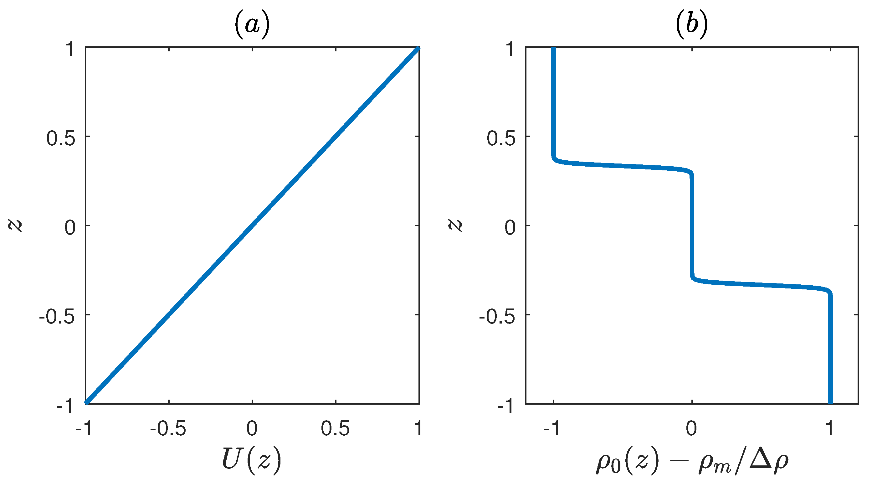The structure of the most unstable mode is shown in Figure 3a,b and exhibits the familiar tilt of the streamfunction against the shear, while there is no discontinuity of the streamfunction at the critical layer $z=0$.

The second branch for higher values of J has modes with growth rates that are approximately one order of magnitude smaller than the growth rates of the modes in the TCI branch and also have non-zero phase speeds. The two complex conjugate eigenvalues for each mode in this branch, correspond to two counter-propagating waves that are similar to the higher-order Holmboe instabilities found by previous studies [36,59]. Their phase speeds shown in Figure 2b are very close to the phase speeds $c_t^{-}$ for $J\simeq 1$ and $c_t^{+}$ for $J\simeq 2$ of the neutral modes in the $R\to \infty$ limit. However, these modes are rendered unstable by the smooth density gradients and were referred to as “overtones” as they are caused by resonances of higher order gravity edge-wave harmonics [30]. The structure of one of these modes is shown in Figure 3c,d. We observe that it is markedly different from the mode in the TCI branch, as it is centered around one of the regions of large density gradients (the oppositely propagating wave is centered around the other). We also note that similar to the TCI modes, there is no discontinuity of streamfunction at the critical layer but this layer becomes evident by the concentration of the density perturbation around it. In addition, according to the diagnostic developed by Eaves and Balmforth [24], which is based on the contribution of vorticity and density to the pseudomomentum of the modes, these modes are characterized as Taylor–Caulfield modes since vorticity does not contribute to their pseudomomentum. We therefore interpret them as overtone TCI modes, even though they are propagating and the streamfunction as well as the vorticity of the modes appears to be concentrated around one of the two density interfaces.

4. Non-Modal Growth of Perturbations

Apart from modal exponential growth, the non-normality of the dynamical operator can give rise to transient non-modal growth of perturbations that can in turn lead to turbulence and mixing. It is therefore of interest to calculate the initial conditions yielding the largest energy growth over a specified time interval $T_{opt}$, as well as to quantify the amount of growth achieved. The time interval $T_{opt}$ is physically limited by the time scale of the mean flow changes and is typically in the order of 1-100 advective time units. The amount of growth is quantified by specifying a norm for the perturbation amplitude. In this work, we follow previous studies [46,48] and consider the perturbation energy density,

$$E\left(t\right)=\frac{1}{2}{\int }_{-1}^1\left(\overline{|{\mathbf{u}}^{\prime }{|}^2}-\frac{J}{(d{\rho }_0/dz)}\overline{{{\rho }^{\prime }}^2}\right)dz,$$

(12)

where the overbar denotes an average over a horizontal wavelength, as the positive definite norm quantifying growth. We also note that, while a different choice of norm can be made, E has the advantage that it is conserved in the absence of a mean flow.

To address transient growth, we rewrite the energy in terms of the state vector as $E\left(t\right)={\widehat{\mathbf{x}}}^{†}\mathbf{M}\widehat{\mathbf{x}}$, where

$$\mathbf{M}=-\frac{\delta z}{4}\left(\begin{array}{cc}\mathrm{\Delta }& 0\\ 0& J/(d{\rho }_0/dz)\end{array}\right),$$

(13)

is the energy norm, $\delta z$ is the grid spacing and the dagger denotes the Hermitian transpose. We transform the dynamics into energy coordinates $\widehat{\mathbf{y}}={\mathbf{M}}^{1/2}\widehat{\mathbf{x}}$, where ${\mathbf{M}}^{1/2}$ is the Cholesky factorization of the energy norm $\mathbf{M}={\mathbf{M}}^{1/2}{\left({\mathbf{M}}^{1/2}\right)}^{†}$. In these coordinates, the energy is given by the Euclidean norm of the state vector and the dynamics is governed by the operator ${\mathbf{A}}_M={\mathbf{M}}^{-1/2}{\mathbf{AM}}^{1/2}$. The optimal perturbations giving rise to the largest energy growth,

$$G\left(T_{opt}\right)=\frac{E\left(T_{opt}\right)}{E\left(0\right)},$$

(14)

over an interval $T_{opt}$ are then calculated through a singular value decomposition of the propagator $e^{{\mathbf{A}}_M{T}_{opt}}=\mathbf{U}\mathbf{\Sigma }{\mathbf{V}}^{†}$, where $\mathbf{U}$, $\mathbf{V}$ are unitary matrices and $\mathbf{\Sigma }$ is a diagonal matrix with the singular values along its diagonal. The optimal growth is the square of the largest singular value of the propagator, while the optimal perturbation is the corresponding column of $\mathbf{V}$ [38].

The main physical mechanism underlying transient growth in planar flows is the Orr mechanism [45], which is exemplified by considering an unstratified, unbounded flow. In this case the dynamics reduce to the conservation of vorticity:

$$\left({\partial }_t+ikz\right)\mathrm{\Delta }\widehat{\psi }=0.$$

(15)

The solution obtained by Kelvin [60] and Orr [45] is given in terms of plane waves with time dependent vertical wavenumber:

$$\widehat{\psi }=\frac{k^2+m^2}{k^2+{(m-kt)}^2}\tilde{\psi }\left(0\right)e^{i(m-kt)z}.$$

(16)

The constant phase lines of these Kelvin–Orr waves, rotate clockwise as the vertical wavenumber decreases linearly with time due to shearing of the perturbation. In addition, shearing deforms the perturbation and constantly increases the distance between the constant phase lines for perturbations leaning against the shear ($m>0$). To compensate for the decreasing distance and conserve vorticity, the amplitude of the streamfunction increases (e.g., Equation (16)) leading to energy growth. The energy amplification continues until the phase lines of the waves become vertical at $t=m/k$. Subsequently, their energy decays as the time dependent wavenumber becomes negative and shearing decreases the distance between the phase lines. Therefore, the optimal perturbations have an initial tilt $m/k=T_{opt}$, such that their phase lines become vertical at $T_{opt}$ and achieve a growth equal to $G_{Orr}\left(T_{opt}\right)=1+T_{opt}^2$ [61]. From the geometric point of view of non-normality, this growth arises due to the properties of the linear operator ${\mathbf{A}}_M$, which has a continuous spectrum of singular modes with eigenvalues $kc$ and eigenfunctions

$$\widehat{\psi }\sim e^{-k|z-c|},$$

(17)

centered around $z=c$. As these modes are non-orthogonal in the energy norm, an initial perturbation can have a very large projection on some of these modes. This large projection is initially masked by the projections onto other modes, thereby yielding an order one initial norm. However, as the perturbation evolves, the projection is unmasked yielding a large norm and producing growth [38]. In the presence of boundaries, the growth achieved as a function of wavenumber is shown in Figure 4a. We observe that, for large wavenumbers, $G_0$ asymptotically reaches the value of growth for the unbounded flow. The reason is that for large k, most of the singular modes have the form of (17) rapidly decaying away from $z=c$ and are unaffected by the boundaries at $\left|z\right|=1$. In contrast, singular modes with lower wavenumbers have a slower decay with height and are significantly affected by the boundaries producing lower growth.

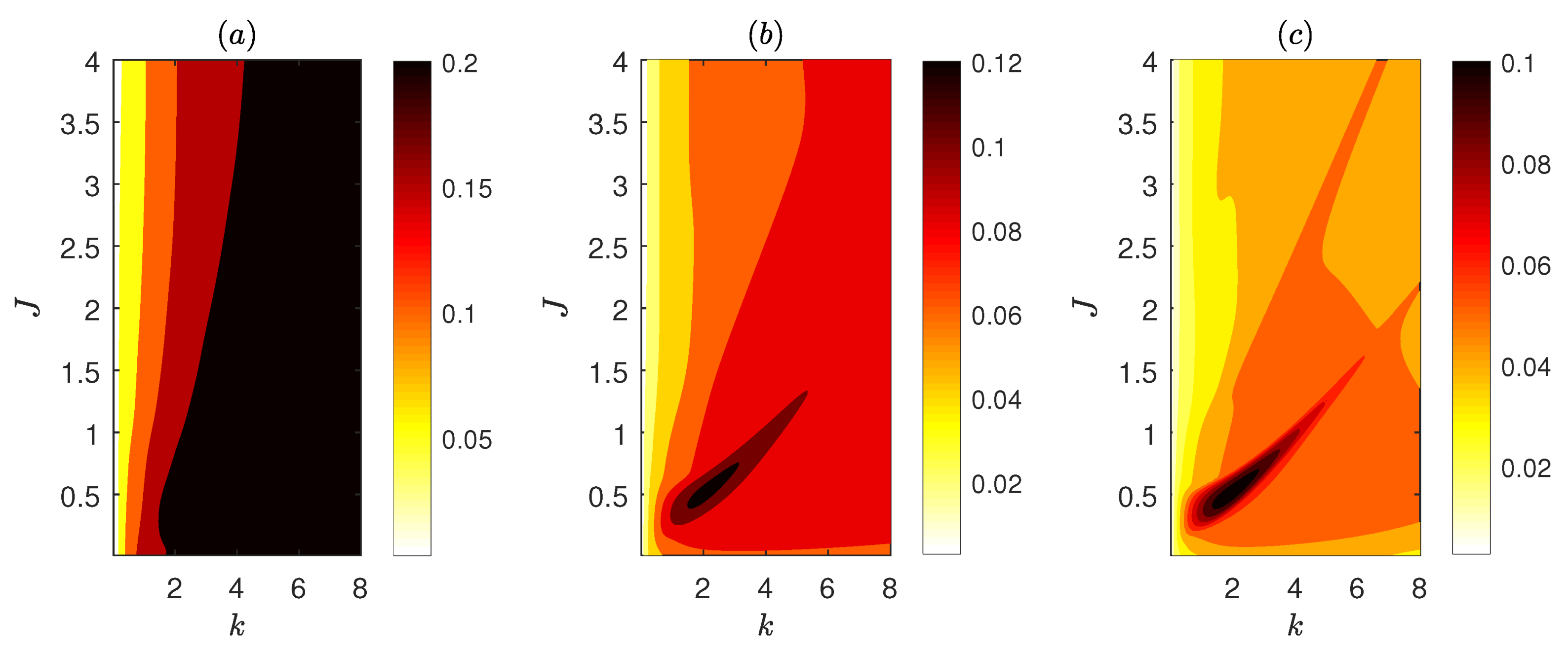
For $J\ne 0$, the energy growth achieved for low optimization times ($T_{opt}=5$) is shown in Figure 4b as a function of wavenumber k and bulk Richardson number J. We observe that, for such low optimization times, the growth achieved is very weakly dependent on the bulk Richardson number for $J⪆2$ and increases with wavenumber, asymptoting to a constant value. This value is approximately equal to $G_0$ as revealed in Figure 4c illustrating the ratio of the optimal growth to the corresponding growth for an unstratified flow. Therefore for early times, the kinetic energy growth produced by the Orr mechanism underlies the transient growth even for the stratified three-layer flow.

Figure 5 shows the finite time Lyapunov exponent $ln\left(G\left(T_{opt}\right)\right)/2T_{opt}$ for larger optimization times. For low wavenumbers, we again observe lower values of optimal growth along with a weak dependence on the Richardson number for $J⪆2$. Maximum growth is achieved either at large wavenumbers for $T_{opt}=10$ or within the TCI branch for larger $T_{opt}$. Note however, that the optimal growth rate in the TCI branch is systematically larger that the modal growth rate shown in Figure 2. The reason is that the optimal perturbation achieving this growth is the initial perturbation with the maximal projection on the unstable mode. For a non-normal operator, this perturbation is not the mode ${\mathbf{w}}_i$ itself, but its bi-orthogonal ${\mathbf{w}}_i^{ad}$ [38]. To find this projection, we write an initial perturbation $\mathbf{x}\left(0\right)$ as the sum of the eigenmodes of ${\mathbf{A}}_M$:

$$\mathbf{x}\left(0\right)=\sum _{i=1}^{2N+1}{\alpha }_i{\mathbf{w}}_i.$$

(18)

The projection coefficients ${\alpha }_i$ can be calculated by utilizing the orthogonality between ${\mathbf{w}}_i$ and ${\mathbf{w}}_i^{ad}$, as for a non-normal operator the orthogonal to the mode ${\mathbf{w}}_i$ with eigenvalue ${\lambda }_i$ is the bi-orthogonal mode ${\mathbf{w}}_i^{ad}$ of the adjoint operator ${\mathbf{A}}_M^{†}$ corresponding to the eigenvalue ${\lambda }_i^{\ast }$. As a result, the coefficients ${\alpha }_i$ are given by:

$${\alpha }_i=\frac{{{\mathbf{w}}_i^{ad}}^{†}\mathbf{x}\left(0\right)}{{{\mathbf{w}}_i^{ad}}^{†}{\mathbf{w}}_i}.$$

(19)

The maximum projection on the unstable mode is thus found by substituting the bi-orthogonal as the initial perturbation to yield:

$$p_i=\frac{1}{{{\mathbf{w}}_i^{ad}}^{†}{\mathbf{w}}_i},$$

(20)

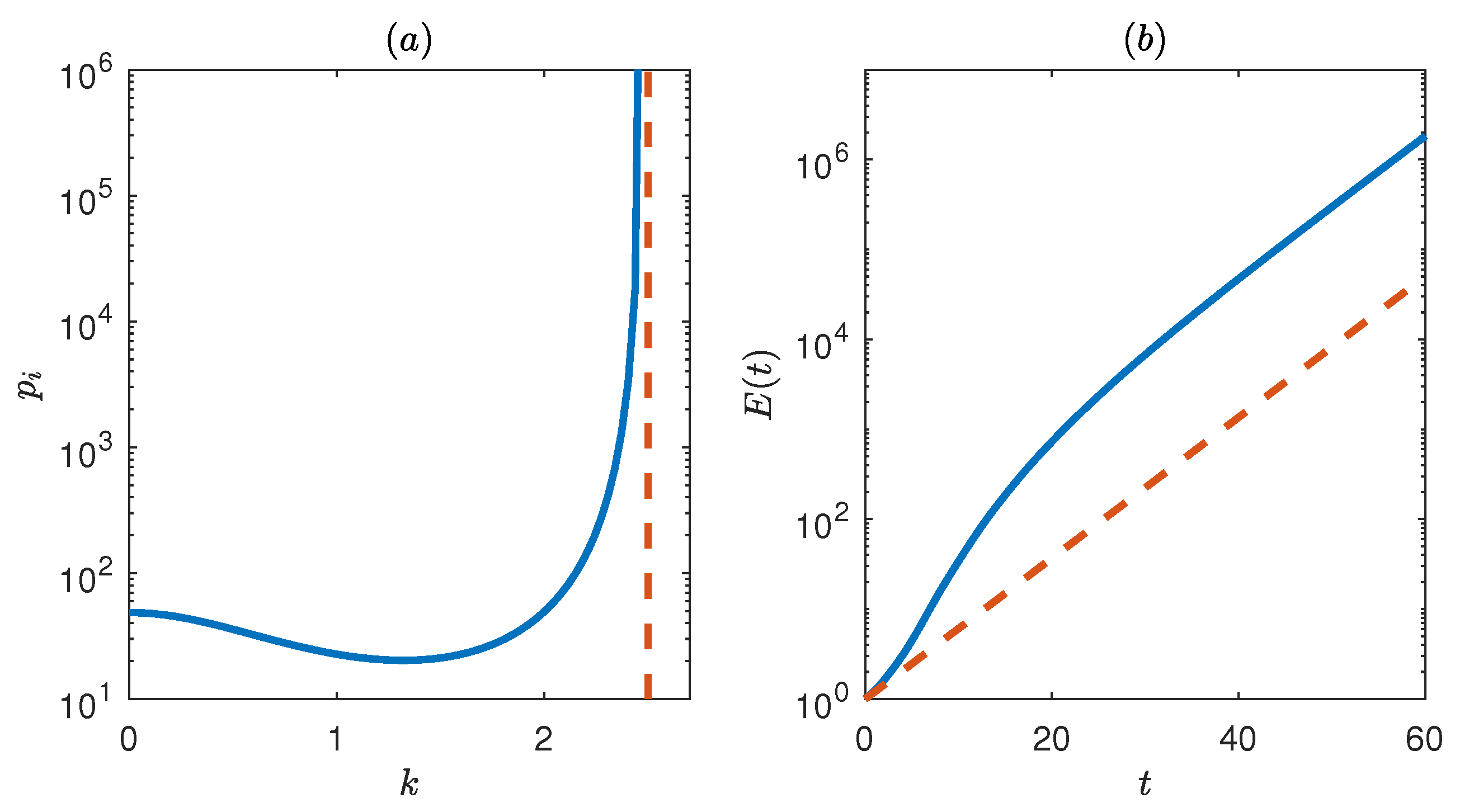
for normalized bi-orthogonal vectors. Figure 6a shows the maximum projection $p_i$ for the unstable modes in the TCI branch, which is the amplified amplitude with which these modes are excited. We observe that the amplified amplitude is of the order of 50 for the most unstable wavenumbers but can reach very high values for wavenumbers close to the cut-off scale of modal instability.

To illustrate the process of the excitation of the unstable mode with increased amplitude, we plot in Figure 6b the energy growth for the bi-orthogonal and compare it with the energy growth of the mode itself. We can see that the energy of both initial perturbations grows at large times exponentially with the same rate $2{\lambda }_i$, but during the early stages of evolution there is an initial boost for the energy of the bi-orthogonal. Figure 7 shows snapshots of the streamfunction during this early stage of evolution of the bi-orthogonal. We observe that the bi-orthogonal shown in Figure 7a has a higher tilt compared to the unstable mode shown in Figure 3a. As it is sheared over (Figure 7b), it is able to achieve rapid transient growth for early times through the Orr mechanism until it assumes the form of the normal mode (Figure 7c). For wavenumbers close to the cut-off scale, the initial growth phase lasts longer yielding larger growth and larger projections. Asymptotically close to the modal marginal stability, the duration of the growth phase tends to infinity along with the growth due to the Orr mechanism and leads to infinite values for the projection (cf. Figure 6a). Therefore, we conclude that, for wavenumbers in the TCI branch, the bi-orthogonals utilize the Orr mechanism to excite the unstable normal modes at large amplitude.

More importantly though, we observe in Figure 5 that there is transient growth even for exponentially stable modes. Such growth is lower compared to the corresponding growth within the TCI branch, but is nevertheless significant. Comparison with the optimal growth for an unstratified flow revealed that it can be up to five times larger than $G_0$ for $T_{opt}=50$ and up to 30 times larger for $T_{opt}=100$, showing that the perturbations take advantage of the interactions between the Kelvin–Orr waves and the gravity edge-waves to produce more growth compared to the unstratified Orr dynamics.

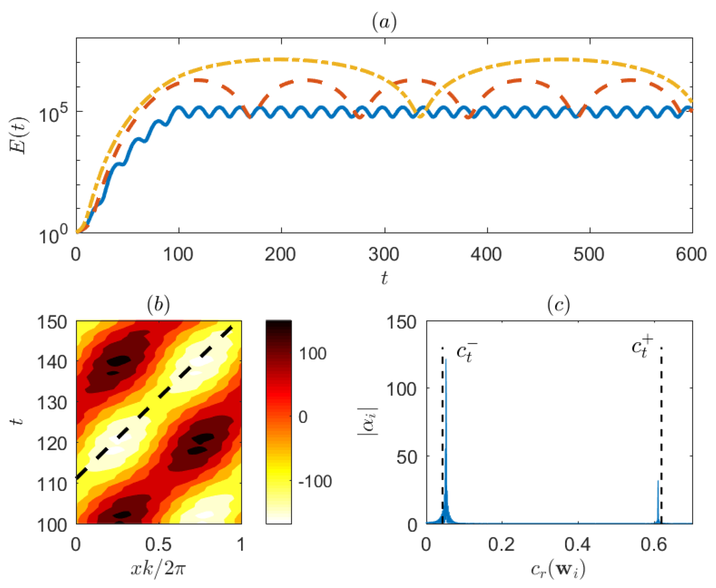
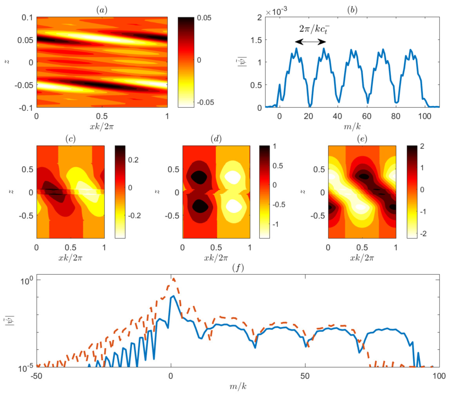
This synergistic action is evident in the evolution of the optimal perturbation in this case which is shown in Figure 8a. We observe a large energy amplification until $T_{opt}$ as would be expected by the Orr dynamics with an equipartition of the energy between kinetic and potential forms (not shown). However, instead of an energy decay after $t=T_{opt}$ we observe a large energy oscillation which is also present at lower amplitude in the amplifying stage. This oscillation is produced by the excitation of propagating waves that are shown in Figure 8b where the streamfunction at the upper density interface ($z=1/3$) is plotted as a function of x and time t. The tilted alternating bands in streamfunction indicate a wave propagating upstream with a specific phase speed. At the lower density interface, a counterpart to this wave propagating downstream with the same phase speed is also observed (not shown). To examine these waves into detail, we project the optimal perturbation ${\mathbf{v}}_{opt}$ onto the modes of ${\mathbf{A}}_M$ as in (19). Figure 8c shows the projection coefficients ${\alpha }_i$ as a function of the phase speed of the modes ${\mathbf{w}}_i$. We have maximum projection near the phase speeds $c_t^{\pm }$ of the neutral waves in the $R\to \infty$ limit, showing that the optimal perturbation is mainly composed of these neutral modes and a collection of continuous spectrum modes with similar phase speeds. The structure of these waves is similar to the unstable modes in the ’overtone’ branch (not shown) with maximum values of the streamfunction at the two density interfaces and the density perturbation centered around the level $z=c_t^{-}$. We therefore conclude that the initial perturbation excites at very large amplitude neutral waves that are supported by the interaction of the gravity edge-waves at the two density interfaces.

We investigate the excitation of these neutral waves by the Kelvin–Orr waves and plot in Figure 9 the evolution of the optimal perturbation and its discrete Fourier decomposition in z. The optimal perturbation that is shown in Figure 9a has a very high tilt against the shear and it comprises of five bands of large wavenumbers as shown in Figure 9b. The snapshots of the evolution of the streamfunction (Figure 9c–e), as well as the Fourier decomposition of the streamfunction at later times (Figure 9f) reveals that as the perturbation is sheared over, its wavenumbers decrease linearly with time according to the Orr mechanism. For example, as it is shown in Figure 9f after $t=10$ advective time units, the first band of wavenumbers for the initial perturbation that was centered around wavenumber $m=10$ has decreased to zero. As this first band of wavenumbers goes to zero and the perturbation starts to tilt vertically (Figure 9d), the next band of wavenumbers is still in the growing phase and the streamfunction tilts again against the shear after a few advection times (Figure 9e). Therefore the perturbation undergoes another period of growth. During these successive growth periods the amplitude of the neutral waves increases as they are gradually excited.

To understand the spacing of the five bands of wavenumbers that constitute the optimal perturbation, we investigate the late stage of the evolution of the optimal perturbation that occurs after $t=T_{opt}$ and is shown in Figure 10. We observe that the neutral waves at the two interfaces constantly repeat a cycle in which they come in phase (Figure 10a) and out of phase (Figure 10c) as they counter-propagate. In between, as the waves come partially in and out of phase, the streamfunction tilts with the shear (Figure 10b) and against the shear (Figure 10d) leading to energy decay and to energy growth of the perturbation respectively. The result is the large energy oscillation observed in Figure 8. During the excitation phase for these waves, the energy oscillation induced by the neutral waves and the energy amplification brought by the Kelvin–Orr waves should synchronize in order to achieve maximum growth. To achieve this, the spacing of the five bands of wavenumbers coincides with the period of the excited neutral waves as shown in Figure 9b.

The same phenomenology of neutral wave excitation holds for all other stable regions in the k-J parameter space. The only difference is that when we approach the TCI branch, the phase speed of the neutral modes goes to zero. Therefore, the period of the oscillation increases as shown in Figure 8a illustrating the energy evolution for the optimal perturbations for two other wavenumbers approaching the stability boundary. More importantly, the amplitude of the oscillation increases rapidly.

5. Discussion

In this work, linear non-modal growth of planar perturbations in a constant shear flow with three density layers was examined. Robust growth at a finite time interval was found with maximum growth obtained for modally unstable perturbations and suboptimal but large values of growth obtained for modally stable perturbations. It was also shown that the optimal perturbations utilize the Orr mechanism to either excite the unstable normal modes or a pair of neutral counter-propagating Taylor–Caulfield modes at high amplitude.

This dynamics might play a role in the evolution of the flow even in the non-linear stage. Numerical simulations of TCI have shown that in many cases the elliptical vortices formed by the primary instability are eventually sheared out and decay [23,24]. After this period, there are persistent oscillations in energy associated with the appearance of parasitic waves that are characterized by increased shear and mixing in one of the interfaces. While these waves were interpreted as Holmboe waves, we note that the neutral Taylor–Caulfield modes as well as the unstable overtone modes share similar characteristics. Taking into account the fact that the flow is modified by the elliptical vortices in many of the cases described above and that the growth of the parasitic waves occurs at a finite time interval, we believe that the Orr mechanism that does not depend sensitively on the details of the flow and produces rapid growth at finite time intervals, can play a significant role in the excitation of these waves, whether they are unstable modes of the flow at the given time or not.

A possible avenue for future work would be to extend the analysis to three-dimensional perturbations in a viscous flow. In full three-dimensional dynamics there is an additional transient growth mechanism, the lift-up effect, which involves the tilt-up of the background spanwise vorticity by the cross-stream perturbation velocity to produce a large amplification of the streamwise velocity [62,63]. In addition, three-dimensional unstable modes will appear at least for Richardson numbers approximately lower than $J_{max}$. The reason is that Yih’s theorem [64] establishes that the most unstable modes are two-dimensional only if the maximally growing perturbation at fixed bulk-Richardson number grows slower than the square root of the Richardson number. That is if $f_{\sigma }=ma{x}_k\left(\sigma \right)/\sqrt{J}$ is a decreasing function of J. Calculation of $f_{\sigma }$ reveals that the criterion is satisfied for $J⪆0.4$, which means that the maximally growing modal instability is three-dimensional for low Richardson numbers.

Regarding the effect of viscosity on non-modal growth, it is known that for unbounded, unstratified flows, transient growth is bounded. For streamwise independent perturbations, growth is maximized at times of $\mathcal{O}\left(Re\right)$ and is of the order of $\mathcal{O}\left(R{e}^2\right)$, while for planar perturbations growth is maximized at times of $\mathcal{O}\left(R{e}^{1/3}\right)$ and is of the order of $\mathcal{O}\left(R{e}^{2/3}\right)$ [39]. We therefore expect that stable or unstable modes including those in the new branch that appears in the presence of viscosity [23], would be excited at amplitudes of that magnitude. However, the exact interplay of the Orr and the lift-up mechanisms in producing growth and in the excitation of normal modes remains to be seen in a future work.

References

1. Caulfield, C.P. Layering, Instabilities, and Mixing in Turbulent Stratified Flows. Annu. Rev. Fluid Mech. 2021, 53, 113–145. [Google Scholar] [CrossRef]
2. Helmholtz, H.V. On discontinuous movement of fluids. Philos. Mag. 1868, 36, 337–346. [Google Scholar] [CrossRef]
3. Kelvin, L. Hydrokinetic solutions and observations. Philos. Mag. 1871, 42, 362–377. [Google Scholar]
4. Rayleigh, L. On the stability, or instability, of certain fluid motions. Proc. Lond. Math. Soc. 1880, 11, 57–70. [Google Scholar] [CrossRef]
5. Drazin, P.G.; Reid, W.H. Hydrodynamic Stability; Cambridge University Press: Cambridge, UK, 1981. [Google Scholar]
6. Thorpe, S.A. Experiments on instability and turbulence in a stratified shear flow. J. Fluid Mech. 1973, 61, 731–751. [Google Scholar] [CrossRef]
7. Caulfield, C.P.; Peltier, W.R. The anatomy of the mixing transition in homogeneous and stratified free shear layers. J. Fluid Mech. 2000, 317, 179–193. [Google Scholar] [CrossRef]
8. Mashayek, A.; Peltier, W.R. The ‘zoo’ of secondary instabilities precursory to stratified shear flow transition. Part 1. Shear aligned convection, pairing and braid instabilities. J. Fluid Mech. 2012, 708, 5–44. [Google Scholar] [CrossRef]
9. Mashayek, A.; Peltier, W.R. The ‘zoo’ of secondary instabilities precursory to stratified shear flow transition. Part 2. The influence of stratification. J. Fluid Mech. 2012, 708, 45–70. [Google Scholar] [CrossRef]
10. Holmboe, J. On the behavior of symmetric waves in stratified shear layers. Geofys. Publ. 1962, 24, 67–113. [Google Scholar]
11. Lawrence, G.A.; Browand, F.K.; Redekopp, L.G. The stability of a sheared density interface. Phys. Fluids A Fluid Dyn. 1991, 3, 2360–2370. [Google Scholar] [CrossRef]
12. Thorpe, S.A. Experiments on the instability of stratified shear flows: Miscible fluids. J. Fluid Mech. 1971, 46, 299–319. [Google Scholar] [CrossRef]
13. Pouliquen, J.; Chomaz, M.; Huere, P. Propagating Holmboe waves at the interface between two immiscible fluids. J. Fluid Mech. 1994, 266, 277–302. [Google Scholar] [CrossRef]
14. Tedford, E.W.; Pieters, R.; Lawrence, G.A. Symmetric Holmboe instabilities in a laboratory exchange flow. J. Fluid Mech. 2009, 636, 137–153. [Google Scholar] [CrossRef]
15. Smyth, W.D.; Klaassen, G.P.; Peltier, W.R. Finite amplitude Holmboe waves. Geophys. Astrophys. Fluid Dyn. 1988, 43, 181–222. [Google Scholar] [CrossRef]
16. Sutherland, B.R.; Caulfield, C.P.; Peltier, W.R. Internal gravity wave generation and hydrodynamic instability. J. Atmos. Sci. 1994, 51, 3261–3280. [Google Scholar] [CrossRef] [Green Version]
17. Smyth, W.D.; Carpenter, J.R.; Lawrence, G.A. Mixing in symmetric Holmboe waves. J. Phys. Oceanogr. 2007, 37, 1566–1583. [Google Scholar] [CrossRef] [Green Version]
18. Taylor, G.I. Effect of variation in density on the stability of superposed streams of fluid. Proc. R. Soc. A 1931, 132, 499–532. [Google Scholar] [CrossRef] [Green Version]
19. Caulfield, C.P. Multiple linear instability of layered stratified shear flow. J. Fluid Mech. 1994, 258, 255–285. [Google Scholar] [CrossRef]
20. Caulfield, C.P.; Peltier, W.R.; Yoshida, S.; Ohtani, M. An experimental investigation of the instability of a shear flow with multilayered density stratification. Phys. Fluids 1995, 7, 3028–3041. [Google Scholar] [CrossRef]
21. Lee, V.; Caulfield, C.P. Nonlinear evolution of a layered stratified shear flow. Dyn. Atmos. Oceans 2001, 34, 103–124. [Google Scholar] [CrossRef]
22. Balmbforth, N.J.; Roy, A.; Caulfield, C.P. Dynamics of vorticity defects in stratified shear flow. J. Fluid Mech. 2012, 694, 292–331. [Google Scholar] [CrossRef]
23. Eaves, T.S.; Caulfield, C.P. Multiple instability of layered stratified plane Couette flow. J. Fluid Mech. 2017, 813, 250–278. [Google Scholar] [CrossRef] [Green Version]
24. Eaves, T.S.; Balmforth, N.J. Instability of sheared density interfaces. J. Fluid Mech. 2019, 860, 145–171. [Google Scholar] [CrossRef] [Green Version]
25. Phillips, O.M. Turbulence in a strongly stratified fluid—Is it unstable? Deep-Sea Res. 1972, 19, 79–81. [Google Scholar] [CrossRef]
26. Fitzgerald, J.G.; Farrell, B.F. Statistical state dynamics analysis of buoyancy layer formation via the Phillips mechanism in two-dimensional stratified turbulence. J. Fluid Mech. 2019, 864, R3. [Google Scholar] [CrossRef] [Green Version]
27. Brethouwer, G.; Billant, P.; Lindborg, E.; Chomaz, J.M. Scaling analysis and simulation of strongly stratified turbulent flows. J. Fluid Mech. 2007, 585, 343–368. [Google Scholar] [CrossRef] [Green Version]
28. Oglethorpe, R.L.F.; Caulfield, C.P.; Woods, A.W. Spontaneous layering in stratified turbulent Taylor-Couette flow. J. Fluid Mech. 2013, 721, R3. [Google Scholar] [CrossRef]
29. Balmbforth, N.J.; Llewellyn Smith, S.; Young, W.R. Dynamics of interfaces and layers in a stratified turbulent fluid. J. Fluid Mech. 1998, 694, 329–358. [Google Scholar] [CrossRef] [Green Version]
30. Ponetti, G.; Balmforth, T.S.; Eaves, T.S. Instabilities in a staircase stratified shear flow. Geophys. Astrophys. Fluid Dyn. 2018, 112, 1–19. [Google Scholar] [CrossRef]
31. Goldstein, S. On the stability of superposed streams of fluid of different densities. Proc. R. Soc. Lond. Ser. A 1931, 132, 524–548. [Google Scholar] [CrossRef]
32. Bretherton, F.P. Baroclinic instability and the short wave cut-off in terms of potential vorticity. Q. J. R. Meteorol. Soc. 1966, 92, 335–345. [Google Scholar] [CrossRef]
33. Carpenter, J.; Tedford, E.; Heifetz, E.; Lawrence, G. Instability in Stratified Shear Flow: Review of a Physical Interpretation Based on Interacting Waves. Appl. Mech. Rev. 2011, 64, 060801. [Google Scholar] [CrossRef]
34. Heifetz, E.; Bishop, C.H.; Alpert, P. Counter-propagating Rossby waves in the barotropic Rayleigh model of shear instability. Q. J. R. Meteorol. Soc. 1999, 125, 2835. [Google Scholar] [CrossRef]
35. Baines, P.G.; Mitsudera, H. On the mechanism of shear flow instabilities. J. Fluid Mech. 1994, 276, 327–342. [Google Scholar] [CrossRef] [Green Version]
36. Alexakis, A. On Holmboe’s instability for smooth shear and density profiles. Phys. Fluids 2005, 17, 08413. [Google Scholar] [CrossRef] [Green Version]
37. Trefethen, L.N.; Trefethen, A.E.; Reddy, S.C.; Driscoll, T.A. Hydrodynamic stability without eigenvalues. Science 1993, 261, 578–584. [Google Scholar] [CrossRef] [PubMed] [Green Version]
38. Farrell, B.F.; Ioannou, P.J. Generalized Stability. Part I: Autonomous operators. J. Atmos. Sci. 1996, 53, 2025–2040. [Google Scholar] [CrossRef]
39. Schmid, P.J.; Henningson, D.S. Stability and Transition in Shear Flows; Springer: New York, NY, USA, 2001. [Google Scholar]
40. Heifetz, E.; Methven, J. Relating optimal growth to counterpropagating Rossby waves in shear instability. Phys. Fluids 2005, 17, 064107. [Google Scholar] [CrossRef]
41. Guha, A.; Lawrence, G.A. A wave interaction approach to studying non-modal homogeneous and stratified shear instabilities. J. Fluid Mech. 2014, 755, 336–364. [Google Scholar] [CrossRef] [Green Version]
42. Case, K.M. Stability of inviscid plane Couette flow. Phys. Fluids 1960, 3, 143. [Google Scholar] [CrossRef]
43. Lin, C.C. Some mathematical problems in the theory of the stability of parallel flows. J. Fluid Mech. 1961, 10, 430. [Google Scholar] [CrossRef]
44. Kelvin, L. Stability of fluid motion: Rectilinear motion of viscous fluid between two parallel planes. Philos. Mag. 1887, 24, 188–196. [Google Scholar]
45. Orr, W.M. Stability or instability of the steady motions of a perfect fluid. Proc. R. Ir. Acad. 1907, 27, 9–69. [Google Scholar]
46. Farrell, B.F.; Ioannou, P.J. Transient development of perturbations in stratified shear flow. J. Atmos. Sci. 1993, 50, 2201. [Google Scholar] [CrossRef] [Green Version]
47. Bakas, N.A.; Ioannou, P.J.; Kefaliakos, G.E. The Emergence of Coherent Structures in Stratified Shear Flow. J. Atmos. Sci. 2001, 58, 2790–2806. [Google Scholar] [CrossRef] [Green Version]
48. Constantinou, N.C.; Ioannou, P.J. Optimal excitation of two dimensional Holmboe instabilities. Phys. Fluids 2011, 23, 074102. [Google Scholar] [CrossRef] [Green Version]
49. Arratia, C.; Caulfield, C.P.; Chomaz, J.M. Transient perturbation growth in time dependent mixing layers. J. Fluid Mech. 2013, 717, 90–133. [Google Scholar] [CrossRef] [Green Version]
50. Kaminski, A.K.; Caulfield, C.P.; Taylor, J.R. Transient growth in strongly stratified shear layers. J. Fluid Mech. 2014, 758, R4. [Google Scholar] [CrossRef] [Green Version]
51. Park, J.; Billant, P.; Baik, J. Instabilities and transient growth of the stratified Taylor–Couette flow in a Rayleigh-unstable regime. J. Fluid Mech. 2017, 822, 80–108. [Google Scholar] [CrossRef]
52. Jose, S.; Roy, A.; Bale, R.; Iyer, K.; Govindarajan, R. Optimal energy growth in a stably stratified shear flow. Fluid Dyn. Res. 2018, 50, 011421. [Google Scholar] [CrossRef] [Green Version]
53. Bakas, N.A.; Ioannou, B.F. Modal and nonmodal growth of inviscid planar perturbations in shear flows with a free surface. Phys. Fluids 2009, 21, 024102. [Google Scholar] [CrossRef]
54. Mallios, C.; Bakas, N.A. Generalized stability of a shear flow with a free surface with respect to three-dimensional perturbations. Phys. Rev. Fluids 2017, 2, 023901. [Google Scholar] [CrossRef]
55. Heifetz, E.; Guha, A.; Carpenter, J.R. Wave interactions in neutrally stable shear layers: Regular and singular modes, and non-modal growth. Phys. Fluids 2020, 32, 074106. [Google Scholar] [CrossRef]
56. Kaminski, A.K.; Caulfield, C.P.; Taylor, J.R. Nonlinear evolution of linear optimal perturbations of strongly stratified shear layers. J. Fluid Mech. 2017, 825, 213–244. [Google Scholar] [CrossRef] [Green Version]
57. Vitoshkin, H.; Gelfgat, A. Non-Modal Three-Dimensional Optimal Perturbation Growth in Thermally Stratified Mixing Layers. Fluids 2021, 6, 731–751. [Google Scholar] [CrossRef]
58. Smyth, W.D.; Peltier, W.R. Three-dimensional primary instabilities of a stratified, dissipative, parallel flow. Geophys. Astrophys. Fluid Dyn. 1990, 52, 249–261. [Google Scholar] [CrossRef]
59. Alexakis, A. Marginally unstable Holmboe modes. Phys. Fluids 2007, 19, 054105. [Google Scholar] [CrossRef] [Green Version]
60. Kelvin, L. On the stability of steady and of periodic fluid motion. Philos. Mag. 1887, 23, 459–464. [Google Scholar]
61. Farrell, B.F.; Ioannou, P.J. Optimal excitation of three-dimensional perturbations in viscous constant shear flow. Phys. Fluids A 1993, 5, 1390–1400. [Google Scholar] [CrossRef] [Green Version]
62. Ellingsen, T.; Palm, E. Stability of linear flow. Phys. Fluids 1975, 18, 487–488. [Google Scholar] [CrossRef]
63. Landahl, M.T. A note on an algebraic instability of inviscid parallel shear flows. J. Fluid Mech. 1980, 98, 243–251. [Google Scholar] [CrossRef]
64. Yih, C.S. Stability of two-dimensional parallel flows for three-dimensional disturbances. Q. J. Appl. Maths 1955, 12, 434–435. [Google Scholar] [CrossRef] [Green Version]
Figure 1. (a) The non-dimensional mean flow velocity U ( z ) = z . (b) The non-dimensional mean flow density ρ 0 ( z ) ρ m / Δ ρ with R = 30 .
Fluids 06 00442 g001
Figure 2. (a) Growth rate of the most unstable modes as a function of wavenumber k and bulk Richardson number J. Also shown is the line J = 2 k / 9 for which resonance in the long-wave limit between the gravity edge-waves supported at the interfaces of sharp density gradient is achieved. (b) Phase speed of the most unstable modes with k = 2 as a function of J (solid line). Also shown are the phase speeds c t + (dashed line) and c t (dash-dotted line) of the neutral modes in the R limit.
Fluids 06 00442 g002
Figure 3. Streamfunction (a) and density (b) for the most unstable mode in the TCI branch with k m a x = 1.9 and J m a x = 0.5 . Streamfunction (c) and density (d) for the most unstable mode in the ‘overtone’ branch with k = 2.6 and J = 1.7 . Also shown in all panels are the interfaces of large density gradients (dashed lines) and the critical layers of the two modes (dashed-dotted) lines.
Fluids 06 00442 g003
Figure 4. (a) Optimal growth G 0 at T o p t = 5 for an unstratified flow as a function of wavenumber. Also shown is the corresponding growth for an unbounded shear flow 1 + T o p t 2 . (b) Optimal growth G at T o p t = 5 as a function of wavenumber and bulk Richardson number. (c) Ratio of the optimal growth G at T o p t = 5 over the corresponding growth for an unstratified flow ( G 0 ) as a function of wavenumber and bulk Richardson number.
Fluids 06 00442 g004
Figure 5. Finite time Lyapunov exponent ln ( G ( T o p t ) ) / 2 T o p t as a function of wavenumber and bulk Richardson number for (a) T o p t = 10 , (b) T o p t = 50 and (c) T o p t = 100 .
Fluids 06 00442 g005
Figure 6. (a) Excitation amplitude p i for the unstable modes in the TCI branch by their bi-orthogonals. Also shown is the cut-off scale for the TCI branch (dashed line). (b) Energy evolution for the bi-orthogonal as an initial perturbation (solid) and for the most unstable mode as an initial perturbation (dashed).
Fluids 06 00442 g006
Figure 7. (a) Streamfunction of the bi-orthogonal to the most unstable mode for k m a x and J m a x . (b,c) Snapshots of the streamfunction at (b) t = 4 and (c) t = 20 showing the evolution of the bi-orthogonal. In all panels the interfaces of large density gradients are also shown (dashed lines).
Fluids 06 00442 g007
Figure 8. (a) The evolution of the energy of the optimal perturbations with k = 3 (solid line), k = 2.5 (dashed line) and k = 2.475 (dash-dotted line). The bulk Richardson number is J = 0.5 and T o p t = 100 . (b) Hovmöller diagram of the streamfunction of the optimal perturbation for k = 3 . That is, contours of [ ψ ^ ( z = 1 / 3 , t ) e i k x ] as a function of x and t for the optimal perturbation. Also shown (dashed line) is the phase speed of the mode onto which the optimal perturbation projects (see panel (c)). (c) Projection coefficients of the optimal perturbation for k = 3 on the normal modes and the continuous spectrum modes. Also shown (dashed lines) are the c t ± phase speeds of the neutral normal modes in the R limit.
Fluids 06 00442 g008
Figure 9. The evolution of the optimal perturbation for k = 3 , J = 0.5 and T o p t = 100 . (a) The streamfunction of the optimal perturbation. (b) The absolute value of the Fourier amplitude of the streamfunction obtained through a discrete Fourier transform. Note that the minimum wavenumber is π leading to the jagged appearance of the line. (ce) Snapshots of the streamfunction at (c) t = 10 , (d) t = 23 and (e) t = 29 . (f) The absolute value of the Fourier amplitude of the streamfunction at t = 10 (solid line) and t = 29 (dashed line).
Fluids 06 00442 g009
Figure 10. Late stage of the evolution of the optimal perturbation for k = 3 , J = 0.5 and T o p t = 100 . Shown are contours of the streamfunction at (a) t = 100 , (b) t = 105 , (c) t = 111 and (d) t = 114 .
Fluids 06 00442 g010
Publisher’s Note: MDPI stays neutral with regard to jurisdictional claims in published maps and institutional affiliations.