Linear Stability of a Steady Convective Flow between Permeable Cylinders

Abstract

Linear stability analysis of a steady convective flow in a tall vertical annulus caused by nonlinear heat sources is conducted in the paper. Heat sources are generated as a result of a chemical reaction. The effect of radial cross-flow through permeable porous walls of the annulus is analyzed. The problem is relevant to biomass thermal conversion. The base flow solution is obtained by solving nonlinear boundary value problem. Linear stability analysis is performed, using collocation method. The calculations show that radial inward or outward flow has a stabilizing effect on the flow, while the increase in the Frank–Kamenetskii parameter (proportional to the intensity of the chemical reaction) destabilizes the flow. The increase in the Reynolds number based on the radial velocity leads to the appearance of the second minimum on the marginal stability curves. The rate of increase in the critical Grashof number with respect to the Reynolds number is different for inward and outward radial flows.

1. Introduction

The analysis of instability of a steady convective flow generated by internal heat sources is important for many problems in science and engineering. The stability of a steady convective flow in an annulus caused by heat sources with constant density is analyzed in [1]. The case of heat sources of non-uniform density is considered in [2,3]. It is shown in these papers that for annual flow, two types of instability exist: (a) shear instability and (b) buoyant instability, discovered earlier in [4,5] for the vertical planar layer and circular pipe, respectively. Recent interest in biomass thermal conversion [6,7] stimulated research in the stability of flows driven by nonlinear heat sources. The base flow solution in this case cannot be found analytically as in many classical problems in hydrodynamic stability (see [8], for example). Bifurcation theory [9] can be used to determine the number of solutions and the region in the parameter space where solutions exist. In a recent paper [10], bifurcation theory is used to analyze nonlinear boundary value problem in an annulus. It is found that for each radius ratio, between the radii, there exists the value of the Frank–Kamenetskii parameter $F_{*}$ (proportional to the intensity of the chemical reaction) such that there are two solutions in the domain $0<F<F_{*}$, one solution for $F=F_{*}$ and no solutions in the region of $F>F_{*}$.

The stability of viscous flow between two concentric cylinders with a radial flow through permeable porous walls of the annulus is analyzed in [11]. Such models (in the presence of rotation) are motivated by applications to dynamic filtration devices and vortex flow reactors [12,13]. The stability of such flows is investigated in [14,15,16]. In the case of non-isothermal conditions, the presence of radial flow can alter the perturbation dynamics. The stability of a combined flow caused by internal heat sources with constant density and a radial inflow or outflow between the permeable walls of the annulus is analyzed in [17], where it is shown that radial flow can stabilize or destabilize the convective flow. In a recent study, the linear stability of a flow in porous medium with permeable boundaries in a vertical layer of annular cross-section is analyzed by [18] for the isothermal case and in [19] for the case where the walls of the layer are maintained at different temperatures. It is shown that for non-isothermal case the flow becomes more and more unstable as the aspect ratio increases.

Linear stability of a steady convective flow in an annulus generated by non-homogeneous heat sources is studied in [20]. The effect of nonlinear internal heat sources on the stability boundary of a vertical flow in an annulus is investigated in [21] for both asymmetric and axisymmetric perturbations for wide range of radius ratios, Prandtl numbers and Frank–Kamenetskii parameters (proportional to the intensity of a chemical reaction). Such models are used to investigate processes in biomass thermal conversion. Different factors (as shown experimentally in [22]) affect the process: external electric field, the degree of swirl of the flow, and convection in the chamber. Complex physical processes are analyzed in nature and engineering, using three basic approaches: (a) experimental analysis, (b) numerical modeling ([23]), and (c) stability analysis. In the present paper, we consider linear stability of a steady convective flow in an annulus caused by nonlinear heat sources. In addition, there is a radially inward or outward flow through porous walls of the annulus. In this case, we are looking for flow instability since it results in more intensive mixing and (hopefully) more efficient energy conversion. The stability of a combined flow (vertical flow due to heat sources and radial flow through the walls) is analyzed. Wide gaps are not used in the study; therefore, the linear stability is analyzed with respect to axisymmetic perturbations. The corresponding nonlinear boundary value problem for the base flow is solved numerically. Using the method of normal modes, we reduce the linear stability problem to the solution of a system of ordinary differential equations with variable coefficients. The collocation method based on Chebyshev polynomials is used to discretize the problem. Calculations show that both inward and outward radial flows stabilize the convective flow in the vertical direction. On the other hand, the Frank–Kamenetskii parameter has a destabilizing influence on the flow. It is shown that a second minimum appears on the marginal stability curve as the Reynolds number increases. For larger values of the Reynolds number, the second minimum disappears.

2. Mathematical Formulation of the Problem

Suppose that a viscous incompressible fluid is situated in the region $D=\{R_1<\tilde{r}<R_2,0\le \phi <2\pi ,-\infty <\tilde{z}<+\infty \}$ between two infinitely long concentric cylinders, where $(\tilde{r},\phi ,\tilde{z})$ is a system of cylindrical polar coordinates centered at the axes of the cylinders. The cylinders’ walls are maintained at a constant and equal temperature ${\theta }_0$. Heat is generated inside the annulus, due to the exothermal chemical reaction described by Arrhenius’ law:

$$Q=Q_0{e}^{-E/\left(R\tilde{T}\right)},$$

(1)

where E is the activation energy, R is the universal gas constant, $Q_0$ is a constant and $\tilde{T}$ is the absolute temperature. Models with internal heat generation given by (1) are used in practice in order to describe processes during biomass thermal conversion [20,21,23] with the objective to obtain cleaner and more efficient sources of energy. Instability is a desirable phenomenon in this case since it enhances fluid mixing, which, in turn, leads to more efficient energy conversion. One of the factors that affects the stability characteristics is the radial flow in the transverse direction. We assume that there is a radial inward or outward flow through the permeable walls $\tilde{r}=R_1$ and $\tilde{r}=R_2$. The following convention is used in the paper: the variables with tildes are dimensional while the variables without tildes are dimensionless.

The problem is described by the system of the Navier–Stokes equations under the Boussinesq approximation. The dimensionless form of the system is as follows:

$$\begin{array}{ccc}\hfill \frac{\partial \mathbf{v}}{\partial t}+Gr(\mathbf{v}·\nabla )\mathbf{v}& =& \nabla p+\Delta \mathbf{v}+T{\mathbf{e}}_k,\hfill \end{array}$$

(2)

$$\begin{array}{ccc}\hfill \frac{\partial T}{\partial t}+Gr\mathbf{v}·\nabla T& =& \frac{1}{Pr}\Delta T+\frac{F}{Pr}{e}^T,\hfill \end{array}$$

(3)

$$\begin{array}{ccc}\hfill \nabla ·\mathbf{v}& =& 0,\hfill \end{array}$$

(4)

where $\mathbf{v}$ is the velocity of the fluid, T is the temperature, p is the pressure and ${\mathbf{e}}_k=(0,0,1)$. The Frank–Kamenetskii transformation is used [24] to transform the source term in (1). The idea is to expand the exponent in the Taylor series and take into account only the linear terms of the expansion. The accuracy of the Frank–Kamenetskii transformation is analyzed in [24,25], where it is shown that for typical values of the parameters in (1), the transformation is quite accurate. The advantage of using it is related to the fact that the source term in (3) is mathematically easier to work with than the term in (1).

The following values are chosen as the measures, respectively, of length, $h=(R_2-R_1)/2$, time, $h^2/\nu$, velocity, $g\beta h^{2}R{\theta }_0^2/\left(\nu E\right)$, temperature, $R{\theta }_0^2/E$, and pressure, $\rho g\beta hR{\theta }_0^2/E$. Here, $\rho$ is the density of the fluid, g is the acceleration due to gravity, $\beta$ is the coefficient of the thermal expansion and $\nu$ is the viscosity of the fluid. In addition, we introduce the notations $\eta =R_1/R_2$, $r_1=R_1/h$ and $r_2=R_2/h$.

Equations (2)–(4) admit a steady solution of the following form:

$${\mathbf{v}}_0=(U_0\left(r\right),0,W_0\left(r\right)),T_0=T_0\left(r\right),p_0=p_{01}\left(r\right)+p_{02}\left(z\right).$$

(5)

The radial inflow or outflow through porous cylinders $r=r_1$ and $r=r_2$ is described by the function $U_0\left(r\right)$. It follows from (4) that $U_0\left(r\right)$ satisfies the following equation:

$$\frac{d{U}_0}{dr}+\frac{U_0}{r}=0.$$

Hence,

$$U_0=\frac{D}{r},$$

where D is an arbitrary constant. The boundary conditions are as follows:

$$U_0{|}_{r=r_1}=\frac{Re}{Gr},U_0{|}_{r=r_2}=\frac{Re\eta }{Gr}.$$

(6)

The following four dimensionless parameters are used to describe the problem: the Grashof number, $Gr=g\beta R{\theta }_0^2{h}^3/\left({\nu }^{2}E\right)$, the Prandtl number,$Pr=\nu /\kappa$, the Frank–Kamenetskii parameter, $F=[\left(Q_0{k}_{0}E{h}^2\right)/\left(\kappa R{\theta }_0^2\right)]exp[-E/\left(R{\theta }_0\right)]$, and the radial Reynolds number $Re=Uh/\nu$, where the radial component of the base flow in dimensionless form is given by the following:

$$U_0\left(r\right)=\frac{Re}{rGr}.$$

(7)

Here, U is the velocity of the fluid at $\tilde{r}=R_1$. It follows from (6) that the velocity at the inner boundary (the first boundary condition in (6)) is fixed. In this case, it is required from continuity (Equation (4)) that the second condition in (6) must be satisfied. Radial outflow $(Re>0$) corresponds to the case where fluid enters the domain through the inner boundary $r=r_1$ and leaves it at $r=r_2$. Radial inflow $(Re<0)$ corresponds to the flow in the opposite direction.

Substituting (6) and (7) into (2)–(4), we obtain the system of equations describing the base flow:

$$\begin{array}{ccc}\hfill W_0^{″}+\frac{W_0^{\prime }}{r}(1-Re)+T_0& =& C,\hfill \end{array}$$

(8)

$$\begin{array}{ccc}\hfill T_0^{″}+\frac{T_0^{\prime }}{r}(1-PrRe)+F{e}^{T_0}& =& 0,\hfill \end{array}$$

(9)

where $C=d{p}_{02}/dz$. The function $p_{01}\left(r\right)$ is not determined since it will not be used in sequel.

The boundary conditions are the following:

$$W_0\left(r_1\right)=0,W_0\left(r_2\right)=0,T_0\left(r_1\right)=0,T_0\left(r_2\right)=0.$$

(10)

It is assumed that the annulus is closed so that the total fluid flux through the cross-section of the annulus is zero:

$${\int }_{r_1}^{r_2}r{W}_0\left(r\right)dr=0.$$

(11)

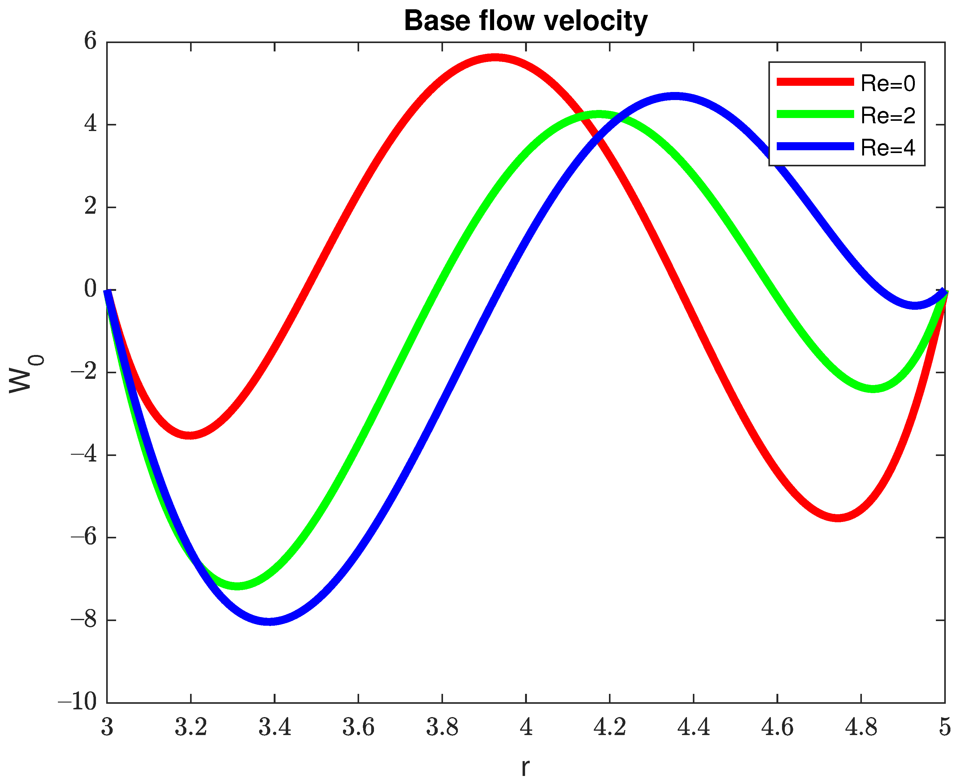
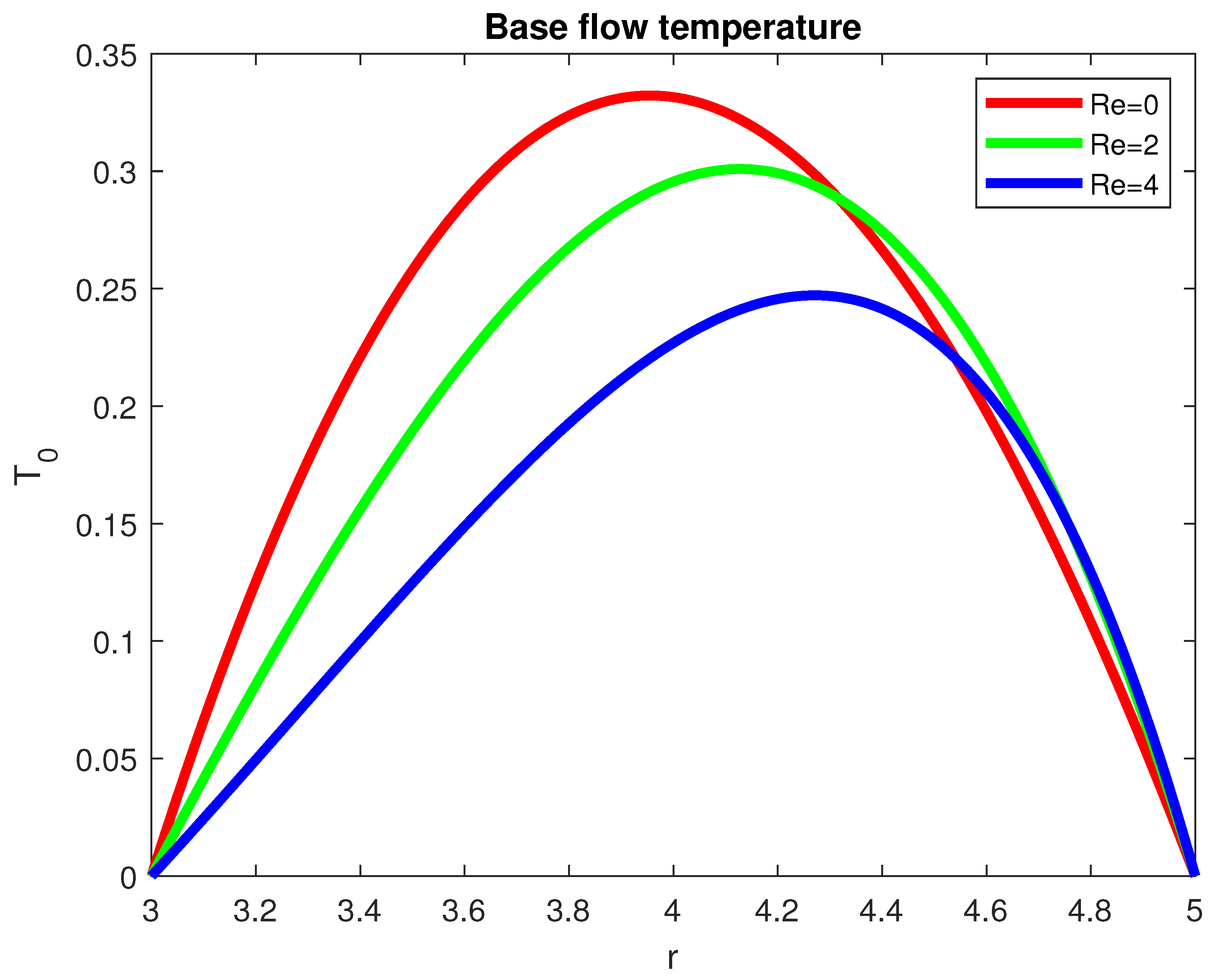
The nonlinear boundary value problem of (8)–(11) is solved, using Matlab routine bvp4c for different values of the parameters, F, $Pr$, and $Re$. The graphs of the base flow velocity and temperature distributions are shown in Figure 1 and Figure 2, respectively, for three values of the Reynolds number. The parameters R and F are fixed at $\eta =0.6$ and $F=0.5$, respectively.

Instability is expected here since the velocity profiles contain inflection points. For $Re=0$, there is one flow upstream in the middle portion of the channel and two flows downstream near the boundaries. As the Reynolds number increases, the intensity of the downstream flow near the outer boundary decreases. Velocity gradients also become smaller as the Reynolds number grows. Thus, it is expected that radial flow will have a stabilizing influence on the stability boundary. This fact is confirmed later by numerical calculations. The base flow temperature distribution becomes more asymmetric as the Reynolds number grows.

3. Numerical Results

Consider a perturbed motion of the following form:

$$\mathbf{v}={\mathbf{v}}^{\prime }+W_0{\mathbf{e}}_k+U_0{\mathbf{e}}_r,T=T^{\prime }+T_0,p=p^{\prime }+p_0,$$

(12)

where ${\mathbf{v}}^{\prime }$, $T^{\prime }$, and $p^{\prime }$ are small unsteady perturbations and ${\mathbf{e}}_r$ is the unit vector in the positive r-direction. Using a standard linearization procedure, we represent the perturbed quantities in the form of axisymmetric normal modes as follows:

$$\begin{array}{ccc}\hfill {\mathbf{v}}^{\prime }(r,z,t)& =& \mathbf{u}\left(r\right)exp(ikz-\lambda t),\hfill \end{array}$$

(13)

$$\begin{array}{ccc}\hfill T(r,z,t)& =& \theta \left(r\right)exp(ikz-\lambda t),\hfill \end{array}$$

(14)

where k is the wave number, $\lambda ={\lambda }_r+i{\lambda }_i$ is a complex eigenvalue and $\mathbf{u}=\left(u\right(r),0,w(r\left)\right)$. The flow (8)–(11) is linearly stable if all ${\lambda }_r>0$ and is unstable if at least one ${\lambda }_r<0$. The flow (8)–(11) is marginally stable if one eigenvalue has ${\lambda }_r=0$, while all other eigenvalues have positive real parts. Eliminating the pressure and longitudinal velocity perturbations from the linearized system, we obtain the following system of ordinary differential equations:

$$\begin{array}{ccc}\hfill u^{\left(4\right)}& +& \left(\frac{2}{r}-U_{0}Gr\right)u^{‴}-\left(\frac{3}{r^2}+2k^2+U_0^{\prime }Gr-U_0\frac{Gr}{r}-ik{W}_{0}Gr\right)u^{″}\hfill \\ & & +\left(\frac{3}{r^3}-\frac{2k^2}{r}-\frac{U_0^{\prime }Gr}{r}+\frac{2U_{0}Gr}{r^2}-ikGr\frac{W_0}{r}+k^{2}Gr{U}_0\right)u^{\prime }\hfill \\ & & +(\frac{2k^2}{r^2}-\frac{3}{r^4}+k^4+\frac{U_0^{\prime }Gr}{r^2}-\frac{2Gr{U}_0}{r^3}-ikGr\frac{W_0^{\prime }}{r}+ikGr\frac{W_0}{r^2}\hfill \\ & & +k^{2}Gr{U}_0^{\prime }+i{k}^{3}Gr{W}_0+ikGr{W}_0^{″})u-ik{\theta }^{\prime }\hfill \\ & & =-\lambda \left(u^{″}+\frac{u^{\prime }}{r}-\frac{u}{r^2}-k^{2}u\right),\hfill \end{array}$$

(15)

$${\theta }^{″}+\frac{{\theta }^{\prime }}{r}-k^2\theta +Fexp\left(T_0\right)\theta -PrGr(u{T}_0^{\prime }+U_0{\theta }^{\prime }+ik{W}_0\theta )=-\lambda Pr\theta .$$

(16)

The boundary conditions are as follows:

$$u\left(r_1\right)=u\left(r_2\right)=0,u^{\prime }\left(r_1\right)=u^{\prime }\left(r_2\right)=0,\theta \left(r_1\right)=\theta \left(r_2\right)=0.$$

(17)

The eigenvalue problem of (15)–(17) is solved numerically, using the collocation method based on Chebyshev polynomials. In particular, the interval $[r_1,r_2]$ is transformed to the interval $[-1,1]$ by means of the following transformation:

$$r=\frac{r_2-r_1}{2}\xi +\frac{r_2+r_1}{2},$$

where $\xi \in [-1,1]$. The functions u and $\theta$ (in terms of the variable $\xi$) are approximated as follows:

$$u\left(\xi \right)=\sum _{m=0}^N{a}_m{(1-{\xi }^2)}^2{T}_m\left(\xi \right),\theta \left(\xi \right)=\sum _{m=0}^N{b}_m(1-{\xi }^2)T_m\left(\xi \right),$$

(18)

where $T_m\left(\xi \right)=cosmarccos\left(\xi \right)$ is the Chebyshev polynomial of the first kind of order m. The collocation points are the following:

$${\xi }_j=cos\frac{\pi j}{N},j=0,1,\dots ,N$$

(19)

In order to estimate the number of collocation points needed for accurate determination of the Grashof number, we performed calculations for one set of parameters, namely, $k=1$, $Pr=2$, $R=0.6$, $Re=2$, $F=0.7$, and different number of collocation points N. The results are shown in

Table 1. The values of the Grashof number $Gr$ for different number of collocation points N.

N	$\mathbf{Gr}$
30	977.416134
40	977.387524
50	977.392292
60	977.392292
70	977.392292

. It is seen from the table that 50 collocation points are sufficient for the calculation of $Gr$, accurate to within 6 decimal places after the decimal point. Similar calculations are performed for other sets of parameters. The calculations show that it is sufficient to use $N=60$ for all cases considered in the paper.

All stability characteristics are calculated below for the case $\eta =0.6$ and $\eta =0.7$. It is shown in [1] that only axisymmetric perturbations are the most unstable for small and moderate gaps, while the first asymmetric mode is the most unstable for the range $0<\eta <0.3$. This is the reason we restrict ourselves with axisymmetric perturbations.

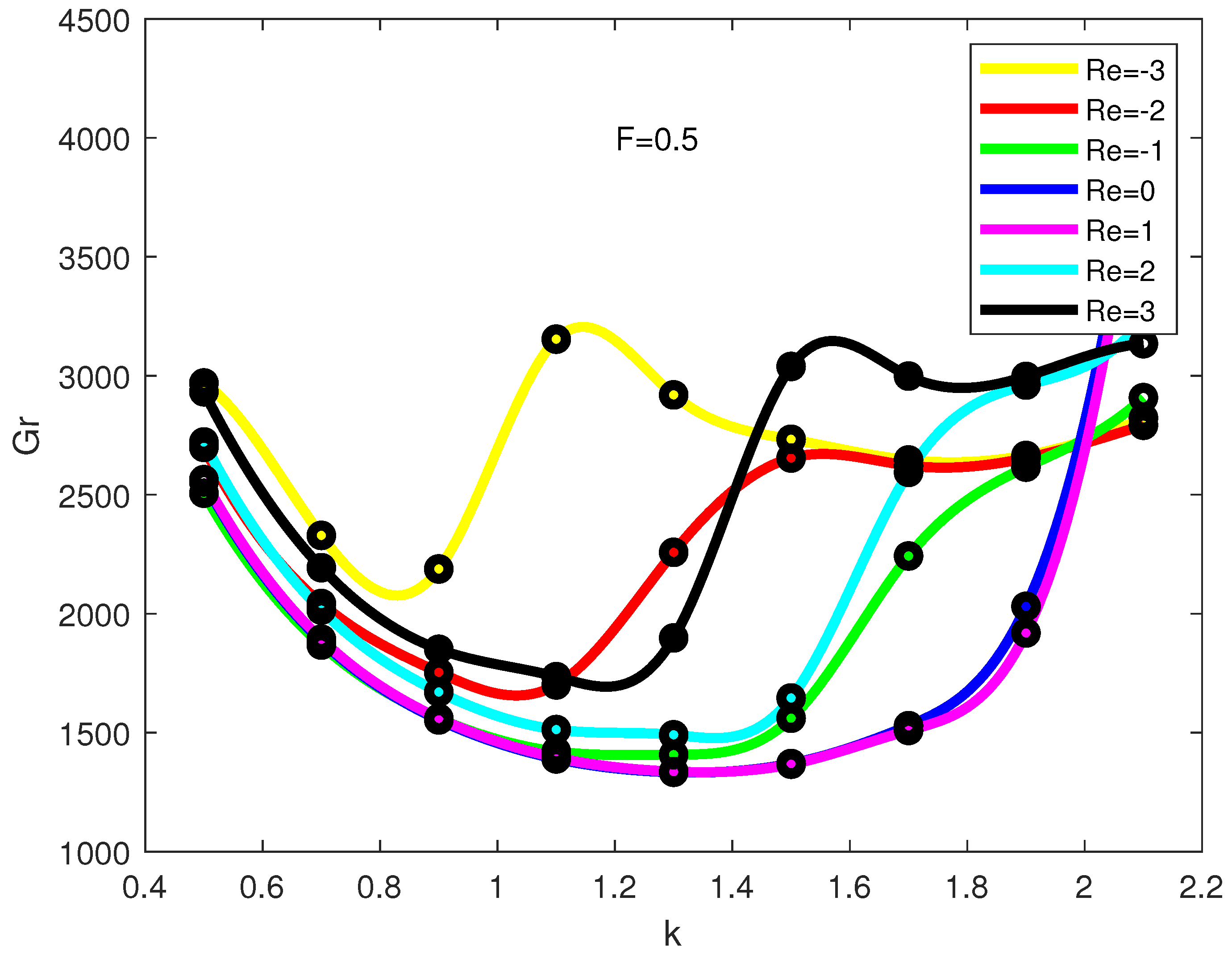
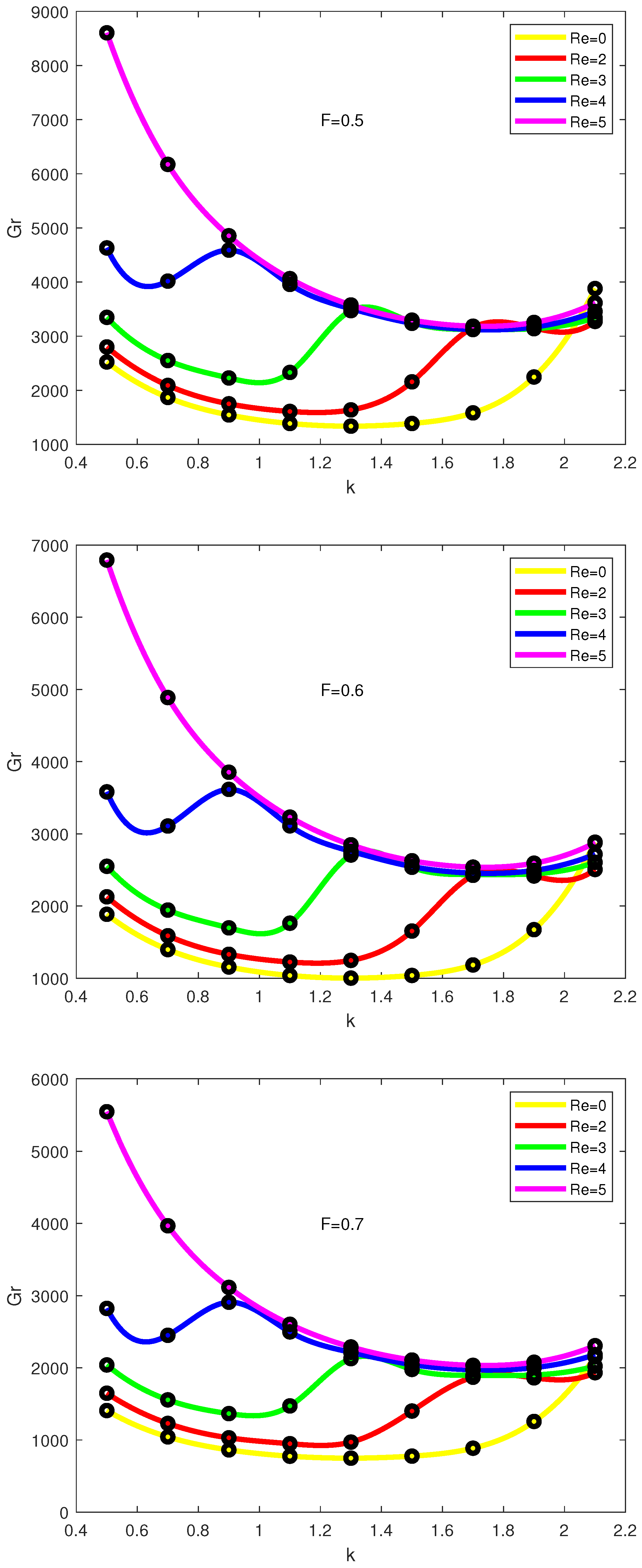
Marginal stability curves for $\eta =0.6$ and different values of F and $Re$ are shown in Figure 3. The dots on the curves correspond to the calculated points, while solid lines are the interpolating curves.The flow is linearly stable in the regions below the curves and unstable in the regions above the curves. On the marginal stability curve, one eigenvalue has zero real part, while all other eigenvalues have positive real parts. The point of an absolute minimum on each marginal stability curve corresponds to the critical values of the parameters $Gr$ and k, denoted by $G{r}_c$ and $k_c$, respectively. Thus, the flow is linearly stable for all k if $Gr<G{r}_c$.

Several conclusions can be drawn from the graphs in Figure 3. First, the increase in F has a destabilizing influence on the flow (the critical Grashof numbers decrease as F increases). Second, for each fixed F, there is a continuous transformation of marginal stability curves as the Reynolds number increases. For $Re=0$ (no radial cross-flow), the marginal stability curve has one minimum. As the Reynolds number increases (see the range $2\le Re\le 4)$, the second minimum appears on the curves. The increase in the Reynolds number (up to $Re=4$) leads to a shift of the minimum point to the region of smaller k. Whether the second minimum is the global minimum depends on the value of the Reynolds number.

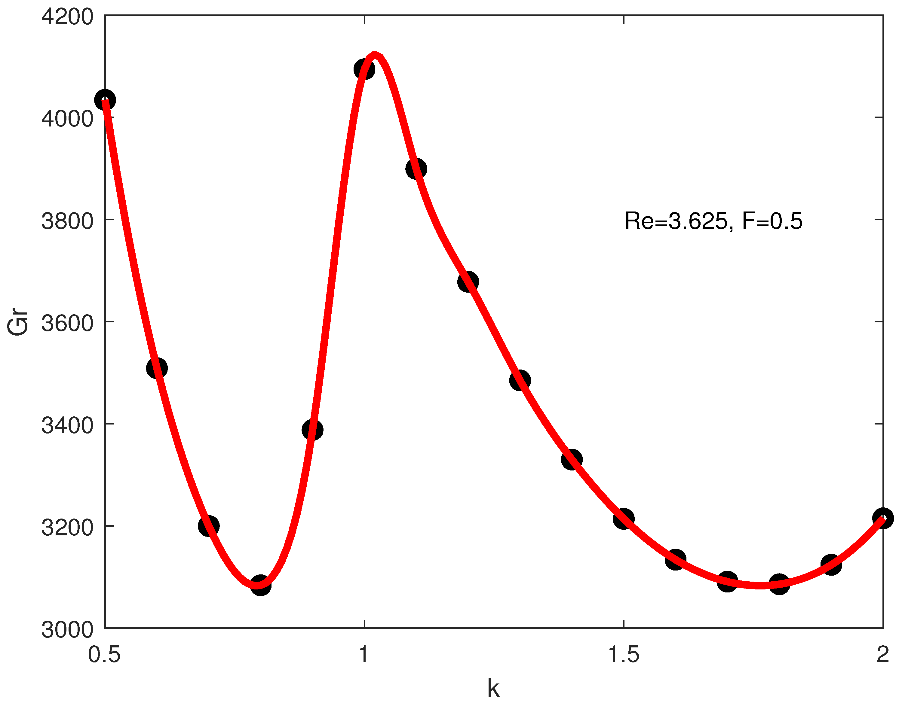
It is seen from Figure 3 that the minimum corresponding to smaller k is the global minimum in the range $0<Re<R{e}_{*}$, where the value of $R{e}_{*}$ depends on F, R, and $Pr$. Calculations show that for the case $\eta =0.6$, $Pr=2$, and $F=0.5$, we have $R{e}_{*}=3.625\dots$ The corresponding marginal stability curve is plotted in Figure 4, where the presence of two equal minima is clearly seen.

The second minimum, which is seen in Figure 3, seems to disappear for higher $Re$. In order to check what happens for larger values of $Re$, we perform calculations for $F=0.5$ in the range $5\le Re\le 11$. The results are shown in Figure 4.

It is seen from Figure 5 that for large $Re$, the marginal stability curves have the same shape as for $Re=0$ (with one minimum). In addition, the increase in $Re$ stabilizes the flow (the critical value $G{r}_c$ increases as $Re$ grows).

The effect of both outward and inward radial flows is investigated further. Figure 6 plots the marginal stability curves for the case $F=0.5$, $\eta =0.7$ and both negative and positive Reynolds numbers. It is seen from the graph that the outward radial flow (positive $Re$) is less stable than the inward radial flow (negative $Re$).

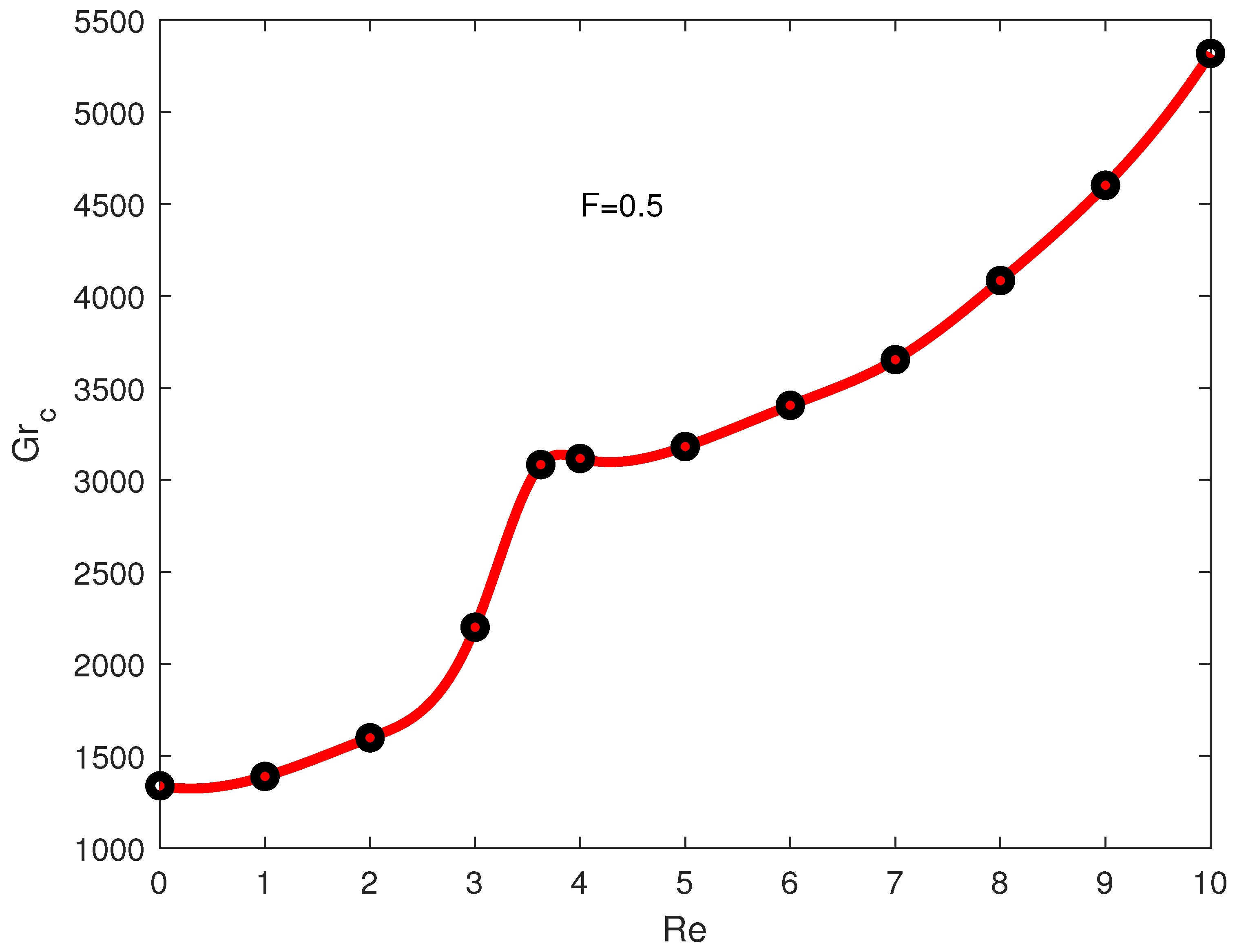
The critical Grashof numbers versus $Re$ are plotted in Figure 7. The Reynolds number has a stabilizing effect on the convective flow since $G{r}_c$ is increasing as $Re$ grows. However, the rate of growth is not the same. The critical Grashof numbers increase faster in the range $0<Re<R{e}_{*}=3.625\dots$ where instability is associated with small wave number perturbations. Then, there is a relatively small growth in $G{r}_c$ for $R{e}_{*}<Re<6$, and then $G{r}_c$ increases faster.

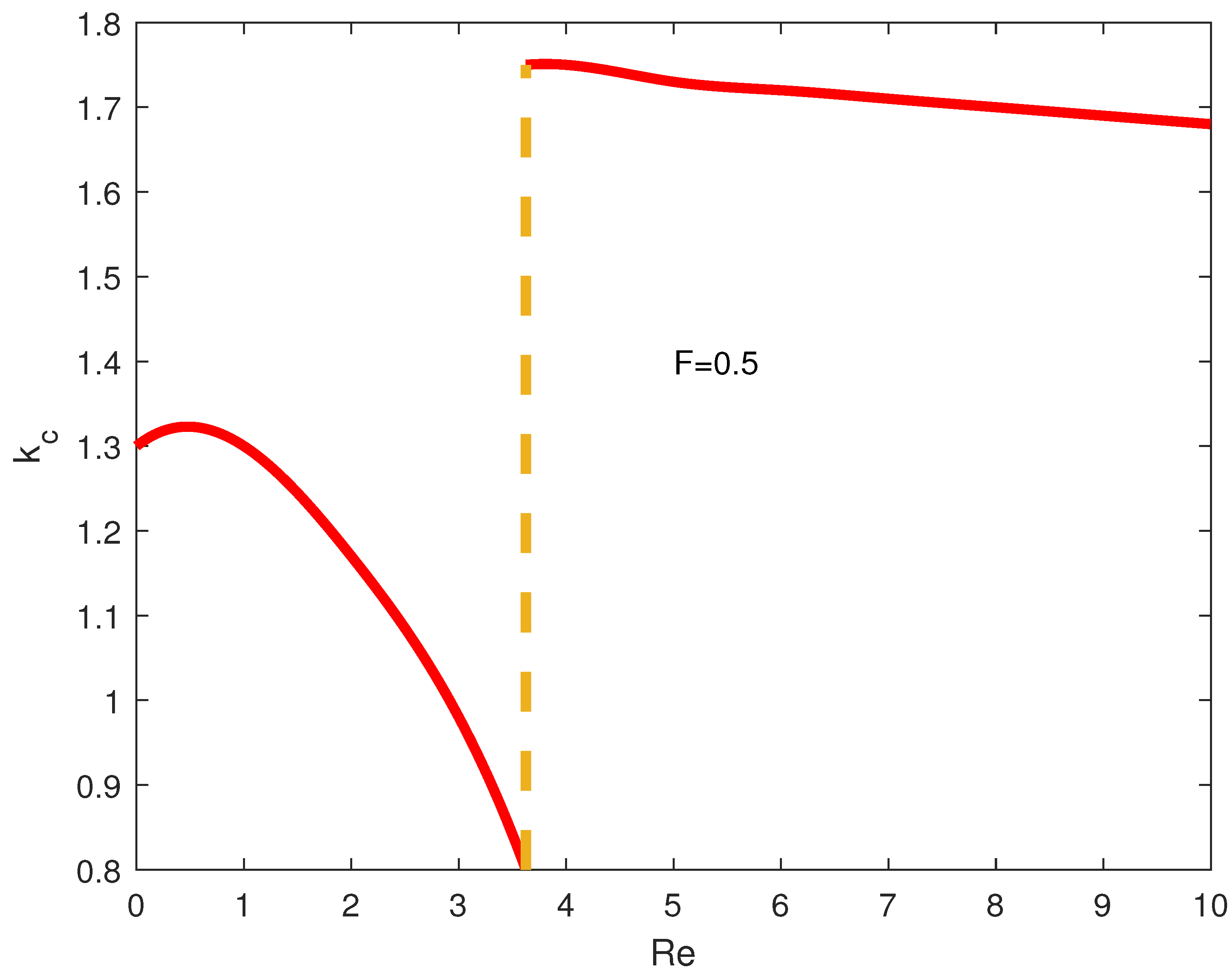
Critical wave numbers versus $Re$ are shown in Figure 8. The finite jump at $Re=R{e}_{*}$ is associated with the transition to perturbations with larger k as indicated in Figure 4.

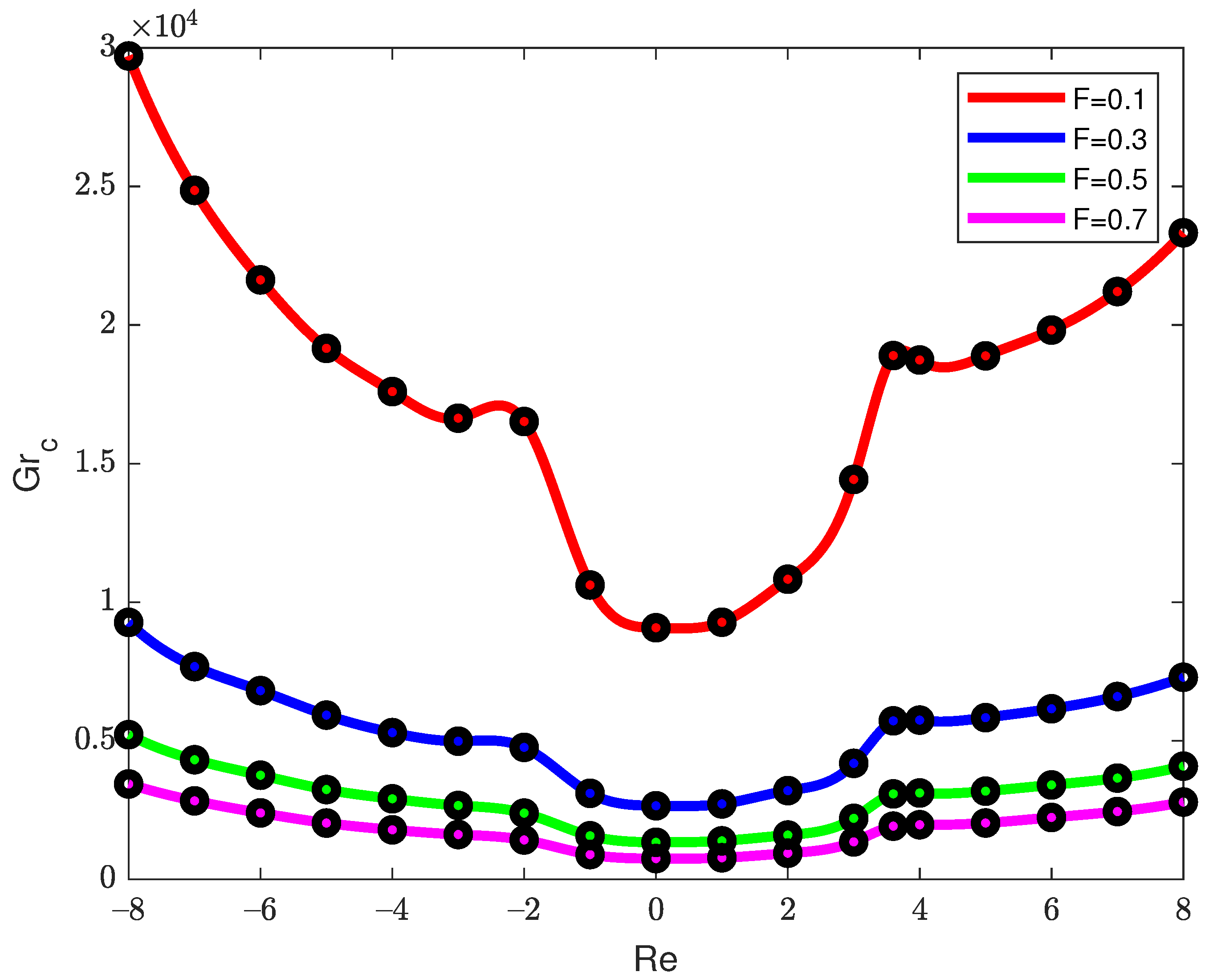
Figure 9 plots the critical Grashof numbers versus positive and negative values of $Re$ in the range $-8\le Re\le 8$ for four different values of the Frank–Kamenetskii parameter F, namely, $F=0.1,0.3,0.5$ and 0.7. The values of R and $Pr$ are fixed at $\eta =0.6$ and $Pr=2$, respectively. Several conclusions can be drawn from the graphs in Figure 9. First, both inward and outward radial flows (negative and positive Reynolds numbers) have a stabilizing influence on the stability boundary. Second, for each F, three different intervals characterizing the rate of increase in the Grashof number with respect to $Re$ can be identified. The first interval (approximately from $Re=-2$ to $Re=3.6$) is associated with relatively strong stabilization of the base flow. The second interval ($Re>3.6$) appears right after the transition to a larger wave number takes place (see Figure 4 and Figure 5 for details). The critical Grashof numbers continue to grow, but at a lower rate. However, as $Re$ increases further, stabilization becomes stronger (the rate of increase in $G{r}_c$ with respect to $Re$ increases). A similar situation takes place around the value $Re=-2$. Here, again, transition to a larger wave number takes place. As a result, the rate of growth of $G{r}_c$ with respect to $Re$ decreases, but then increases again as the Reynolds number becomes more and more negative. Third, the rate of increase in $G{r}_c$ with respect to $Re$ is not the same for positive and negative Reynolds numbers. Fourth, base flow stabilization also depends on the value of the Frank–Kamenetskii parameter F. Stabilization is much stronger for small F (see the graph for $F=0.1$ in Figure 9) and less pronounced for larger F. Fifth, as F increases, the critical Grashof number approaches zero. The last conclusion is consistent with the fact that a steady convective flow in the vertical direction generated by internal heat sources exists only in the range $0<F<F_{*}$ (see [10] for the case $Re=0$), where $F_{*}$ depends on R and $Re$, and there is no steady solution for $F>F_{*}$.

4. Discussion

Linear stability of a steady convective flow caused by nonlinear heat sources in a tall vertical annulus is analyzed in the paper. It is assumed that there is a radial inward or outward flow through the permeable walls of the annulus. The base flow is obtained numerically as a solution of the nonlinear boundary value problem for the system of ordinary differential equations. The linear stability problem is solved by the collocation method for different values of the parameters of the problem. The Prandtl number is fixed at $Pr=2$. Analysis of the base flow velocity profiles suggests that the Reynolds number (proportional to radially inward or outward velocity) will stabilize the flow. This fact is confirmed by calculation of the marginal stability curves. It is shown that the second minimum appears in the region of smaller wave numbers as the Reynolds number increases. This minimum may or may not be the global minimum. However, for large Reynolds numbers, the second minimum disappears. The other parameter that affects stability characteristics is the Frank–Kamenetskii parameter (proportional to the intensity of the rate of a chemical reaction). The increase in the Frank–Kamenetskii parameter destabilizes the flow. In addition, there exists the value $F_{*}$ such that steady flow exists only in the range $0<F<F_{*}$. There is no steady flow in the domain $F>F_{*}$ (this fact is denoted as the thermal explosion in the literature). In the region where steady flow exists, the stability characteristics are determined by the concurrence of the two factors: (a) stabilizing effect of the radial flow (both inward and outward) and (b) destabilizing effect of the intensity of the chemical reaction (the Frank–Kamenetskii parameter).

Wide gaps between the walls of the annulus are not considered in the present study (the values of $\eta$ that are used in the paper are $\eta =0.6$ and $\eta =0.7$). As was shown in [1,20], asymmetric perturbations (depending on the angular coordinate $\phi$) are the most unstable for very large gaps (small values of $\eta$), which is why only axisymmetric perturbations are considered in the present paper. In the future, we plan to investigate the role of the radius ratio on the stability boundary as well as to consider different Prandtl numbers by analyzing both axisymmetric and asymmetric perturbations. In addition, weakly nonlinear theory can be used to analyze the development of instability beyond the threshold. The authors are currently working on these topics.