Abstract
Subsurface multiphase flow in porous media simulation is extensively used in many disciplines. Large meshes with non-orthogonalities (e.g., corner point geometries) and full tensor highly anisotropy ratios are usually required for subsurface flow applications. Nonetheless, simulations using two-point flux approximations (TPFA) fail to accurately calculate fluxes in these types of meshes. Several simulators account for non-orthogonal meshes, but their discretization method is usually non-conservative. In this work, we propose a semi-implicit procedure for general compositional flow simulation in highly anisotropic porous media as an extension of TPFA. This procedure accounts for non-orthogonalities by adding corrections to residual in the Newton-Raphson method. Our semi-implicit formulation poses the guideline for FlowTraM (Flow and Transport Modeller) implementation for research and industry subsurface purposes. We validated FlowTraM with a non-orthogonal variation of the Third SPE Comparative Solution Project case. Our model is used to successfully simulating a real Colombian oil field.
1. Introduction
Subsurface flow in porous media remains an important area in many biological, industrial and scientific applications. Numerical simulations of coupled multiphase-multicomponent flow in porous media, using continuum mechanics approach [1], have been extensively applied in various fields including, hydrology [2,3], soil remediation [4,5], storage [6], oil and gas, composite materials manufacturing [7,8]. One important application is enhanced oil recovery (EOR) in which various multicomponent phenomena arise, e.g., foam transport and generation [9,10], chemical flooding [11,12], in-situ upgrading [13], and asphaltene precipitation [14,15], flocculation, and remediation [16,17]. Due to this high number of applications, and the continuous development of new techniques for EOR based on chemical and thermal processes, robust and flexible numerical simulation frameworks are required to evaluate and optimize the field deployment of such technologies.
The solution of the partial differential equations (PDE) originated from flow and transport models in porous media, is approximated using conservative numerical methods such as finite volume method (FVM) [18,19]. Subsurface spacial domains have complex geometries that are usually modeled by unstructured or non-orthogonal grids (e.g., PEBI grids [20] or corner-point geometries [21,22]). The advective term in FVM is often discretized following the two-point flux approximation (TPFA) [23]. The TPFA is the industry-standard methodology, in which the local K-orthogonality effect must be considered to achieve numerical convergence [24]. Numerical meshes in many cases, have highly anisotropic ratios inducing an additional source of error [25,26]. Consequently, several authors proposed methods for computing numerical gradients at element surfaces to enable accurate solutions with TPFA in non-orthogonal grids [27,28,29,30,31,32], but most of these methods were developed primarily for isotropic tensorial field applications. In most cases, those are limited to 2-dimensional geometries or simple single-phase fluid problems for anisotropic porous media applications [33]. Thus, the numerical method formulation to be developed, must be general, flexible, and easily adaptable to admit the various physical phenomena involved in many environmental, industrial and biological applications in porous materials.
There are currently several simulators in development for multiphase transport in porous media, mainly to subsurface applications. On the industry side, the leading commercial simulators are ECLIPSE [34], GEM [35], and STARS [36], which are used in oil and gas applications. The first uses a finite difference method (FDM); the second and third use FVM with finite differences to approximate the numerical fluxes at the faces. On the other hand, there are research purpose simulators like Finite Element Heat and Mass Transfer Simulator (FEHM) [37] and OpenGeoSys [38]. These are based primarily on the finite element method (FEM), which is also locally non-conservative for any fluid phases, because of the imposed continuity of the solution through element faces [39]. Another more elaborated academic simulators such as Stanford General Purpose Research Simulator (GPRS) [40,41] uses FVM with a multi-point flux approximation (MPFA) technique instead of TPFA to deal with non-orthogonality and full tensor effects in arbitrary polyhedral grids. There are also parallel oriented simulation platforms like Integrated Parallel Accurate Reservoir Simulators (IPARS) [42], which is a framework for developing parallel models of subsurface flow and transport through porous media; and DuMu [43], a compositional simulator built on top of DUNE [44,45], a modular toolbox for solving partial differential equations. Besides, it is worthy of mention Open Porous Media simulator (OPM) [46] and the MATLAB Reservoir Simulation Toolkit MRST [47], designed for rapid prototyping and evaluation for reservoir simulation problems [48]. The last one uses a Mimetic finite difference method (MFDM) to achieve very accurate solutions in unstructured geometries at the cost of higher computational complexity. Moreover, the methodology developed in this paper is the theoretical foundation of FlowTraM (Flow and Transport Modeller), a compositional subsurface flow simulator developed at the National University of Colombia for research purposes in developing and testing new EOR technologies.
In this work, we present an unstructured finite volume method (UFVM), with an improved TPFA, which allows for managing mesh non-orthogonality with full tensor permeability effect. Mesh skewness [49] is taken into account by a direct consequence of our methodology formulation, which is a generalization to the 3-dimensional case of the previous work of Loudyi [32], applied to non-linear multiphase flow. Besides, the loss of convergence rate, due to the K-orthogonality effect, is compensated by introducing additional corrective fluxes in Newton’s method formulation. These corrections, non-orthogonality, and skewness, require gradient reconstruction techniques. This gradient reconstruction is done efficiently by constructing preprocessed stencils in the weighted least-squares sense (WLS). We use a generalized Crank Nicholson scheme [50] (also known as implicit-explicit or IMEX method [51,52]) for time discretization. Furthermore, our semi-implicit procedure serves to approximate the corrective fluxes, taking advantage of the IMEX method formulation, the current time solution, and the internal iterations of Newton’s method for the resulting non-linear algebraic equations system. The discretization presented here for the advective transport term employs the second-order anisotropic elliptic operator [53,54], which enables a trivial extension of the proposed methodology to any physical transport phenomena originated by a gradient law [55] in anisotropic tensorial fields. Also, our methodology conception allows for naturally extending the functionality of already implemented flow simulators based on FVM for cartesian meshes, increasing its functionality to non-orthogonal structured meshes, as is the case for corner point geometries in a natural way.
This paper is organized as follows: First, we present the mathematical model, emphasizing the physical principles of transport phenomena, using a continuum mechanics approach. In this context, the conservation equations for an arbitrary number of components are presented. Subsequently, we show our UFVM formulation, including some remarks about our implementation (FlowTraM). Furthermore, we present three numerical examples, validating our method and verifying the effectiveness of corrective fluxes. Finally, we demonstrate the robustness and flexibility of this numerical approach simulating an actual Colombian reservoir under EOR operation.
2. Mathematical Model
2.1. Transport Models
The total flux of transport of species k in phase p is expressed in terms of pressure, molecular diffusion, mechanical dispersion, and other factors as [55]:
The transport of components in a fluid medium can occur due to the effect of various internal forces [56], which, in general, are a consequence of the presence of gradients, either from pressure, concentration, or temperature [57]. Advection and hydrodynamic dispersion are the main mechanisms dominating transport in porous media [55]. However, other types of effects may be relevant depending on the case study, such as the Soret effect induced by temperature gradients [58,59] or the chemotaxis phenomenon, in which certain types of microorganisms move through the porous medium due to the presence of nutrient concentration gradients [60,61,62]. However, although this work is limited to the modeling of advection transport, the discretization presented here can be extended to any phenomenon expressed by a gradient law. Thus, the transport of species by advection is given by:
where is the molar fraction of the component k in the phase p, and the velocity of each phase given by the Darcy equation for multiphase flow, which establishes a relationship of proportionality with the phase potential as:
and is the symmetric positive definite tensor of absolute permeability, the relative permeability of the phase p and the phase viscosity. The ratio is known as the mobility of the phase p. Additionally, the potential is defined in terms of pressure as:
2.2. Compositional System of Equations
Let an open bounded set and . The system of continuity equations, for number of components, distributed in phases is
where is the family of indices for each component, is the molar flux by advection, and is the number of moles per unit of volume. Additionally, let be open sets such that and , the Neumann, and Dirichlet type boundaries respectively. Equation (5) satisfies the following boundary conditions
Usually, to indicate that the domain is physically closed, in a portion of the boundary, is set, indicating that or that the permeability at the border is zero i.e., . Since Equation (5), subject to boundary conditions (6), models the evolution of the system in time interval , an initial configuration of the variables is required, which is
where is the family of phase indexes. The functions , , and must satisfy the compatibility equations shown in the next section.
The main unknowns of the problem are the pressure functions for each of the phases , the saturations , and the molar fractions of the components distributed in the phases. Including this, the total number of unknowns is , of which term corresponds to the phase, pressure and saturation unknowns, and is the number of unknowns corresponding to the molar fractions.
2.3. Compatibility Equations
Properly speaking, the gradient laws for transport phenomena are compatibility equations, because they satisfy the material objectivity axioms [63]. Nevertheless, they are assumed here as part of the governing equations, and the constitutive relations or compatibility equations are stated as follows:
2.3.1. Thermodynamic Equilibrium
Transport equation terms and particularly their non-linearities are highly related to the thermodynamic state and properties of the existing phases in a specific space-time location. Nowadays, most of the models working with local thermodynamic equilibrium assumption are capable of reproducing a wide range of compositional phenomena in oil and gas reservoirs [64]. This assumption holds as long as exists an appropriate equation of state calibration for the PVT fluid behavior. Adding flexibility to our model, and making it more general for Black-oil type and fully-compositional fluids, the problem of thermodynamic properties determination was decoupled from the conservation equations, being solved sequentially after determination of primary variables. As a general description, thermodynamic equilibrium can be defined mathematically as the equality of fugacities, , of each component k in a mixture for all phases [65].
Fugacity is solved by one of the several equations of state available for hydrocarbon modeling, attached to the following inner constraints:
where is the molar fraction of phase p in a point, and is the global molar fraction of component k in that particular spatial location.
This set of equations is internally solved at each instant and space location, applying the Peng & Robinson [66] equation of state. The solution of such a system is then sequentially coupled to the transport equations, assuring a precise calculation of the involved thermodynamic properties. Considering three pseudo-components gas, oil, and water for an extended black-oil model, a modified version of the Wang [67] approach was used to translate the tabulated PVT information to the compositional formulation.
2.3.2. Capillary Pressure
Capillary pressure equations state a pressure discontinuity between two competing phases, a wetting phase , and a non-wetting phase [68,69,70]. Capillary pressure relationship is expressed as a general functional as follows for two arbitrary wetting and non-wetting phases:
where, capillary pressure equations, one per binary system , are required in a system of multiple phases. The pressure difference between phases is considered for the transport equations but is assumed to be insignificant for thermodynamic equilibrium calculations.
2.3.3. Volume Constraint
The volume constraint equation states that the sum of the volume occupied for each phase is equal to the porous space. Volume constraint equation is as follows:
2.4. Second-Order Anisotropic Elliptic Operator
Most of the transport models can be written in terms of the second-order anisotropic elliptic operator defined as , where is a tensorial property and the scalar function of interest. For an advective model, and .
3. Numerical Model
In this section, we present the discretization for the continuity Equation (5) for advection, using an unstructured finite volume method (UFVM) maintaining the second order of convergence, considering the correction for anisotropy non-orthogonality and skewness.
3.1. Time Discretization and Mesh Definition
For computing an approximation of the solution in time, a discretization of the simulation interval is required first. Let a partition of . Each temporal element or simulation interval is defined as , for .
For spatial discretization, let the physical domain of interest and , with , open, bounded and simply connected subsets in , such that , for all and also
where is the discrete domain, which approximate [71]. The subsets of the partition are denoted as elements or cells [72]. Note that in the context of this definition, when considering the notion of an open set and its closure, is implicitly distinguishing between the interior of the elements and their respective boundaries , which are divided in a finite number of simply connected faces whose boundaries are also known as edges [44,45,73]. Two cells and are neighboring or adjacent if both share a face f, that is, .
3.2. Finite Volume Integral Formulation
The integral form of the continuity equations, in terms of the second-order anisotropic elliptic operator, for advection transport, is obtained by integrating Equation (5) over an arbitrary element and time interval as:
The discretization of each of the terms of Equation (13) is done separately, resulting in the system of nonlinear algebraic equations, which is solved by the Newton method.
Accumulation Term
For the discretization of time derivative is assumed that each element geometry remains constant along with the simulation, and the fluid properties are homogeneous over each element [74]. By applying the Fubini theorem and the fundamental theorem of calculus, the discretization form of the accumulation term is obtained as:
where is the measure of .
3.3. Advective Term
This work focuses mainly on the discretization of this term, considering full permeability tensors and irregular polyhedral elements. The first step is to apply the Green-Gauss theorem to the elliptic operator as follows:
where denotes the inner product in , is the unit vector normal to surface , and is the co-normal vector defined as in which the anisotropy effects reside. To deal with potential field discontinuity due to heterogeneity, the permeability tensor in f is computed in harmonic sense as [32]:
where is the coordinate system direction.
The surface integral in Equation (15) can be interpreted as the net flux of moles of component k, in phase p, across the boundary of the element. Then, as the control volume is a polyhedron defined by a finite number of faces, the surface integral also can be decomposed in a sum over his faces, and the flux en each one is approximated with a second-order midpoint rule [75] as:
where is the face area, and in general, the subscript f indicates that the property, whether scalar or vector, is evaluated at the face centroid . For obtaining the system of algebraic equations, it is necessary to find an approximation of the directional derivative , in terms of the potentials evaluated in the cell centroids.
Let and adjacent elements through the face f with centroids and respectively and the vector that connects these centroids, defined as . Then, vectors and are expressed as a linear combination of the elements of the face orthonormal basis as
where and are unit vectors tangential to the face such that . The geometrical elements defined here are shown schematically in Figure 1. Getting an expression for the normal vector from (18) and replacing it on (19), a vector equation for is obtained in terms of and as
where the coefficients are
and
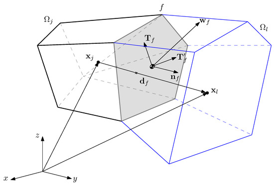
Figure 1.
Scheme of the geometric elements involved in the discretization of the advective term.
Besides, the product is known as shape factor in classical reservoir simulation literature, and it coincides with the formulation of Islam [74], Abou-Kassem [68] and Aziz [69], for rectilinear orthogonal grids. Thus, applying the vector decomposition (20) to the directional derivative at (17) gives the following expression for the advective term:
The tangential component takes account of skewness distortion error, as shown below:
First, using a Taylor series expansion for the potential centered at the face centroid, evaluated at and , yield to expressions for and respectively, in terms of potential partial derivatives as
where and are the residual truncation errors for the Taylor series, and the face-to-cell director vectors are defined as and . Now, subtracting the expressions (25) and (26) result in:
where , and therefore
in which
This work is limited to the case in which the operator is expressed as
Finally, the advective term discretization is
where
3.4. Source/Sink Term
This term is directly associated with the production/injection rate of the component k in the domain. The production rate can be understood as a function, of space and time, whose second-order discretization consists only of the application of the mean value theorem [74] as follows:
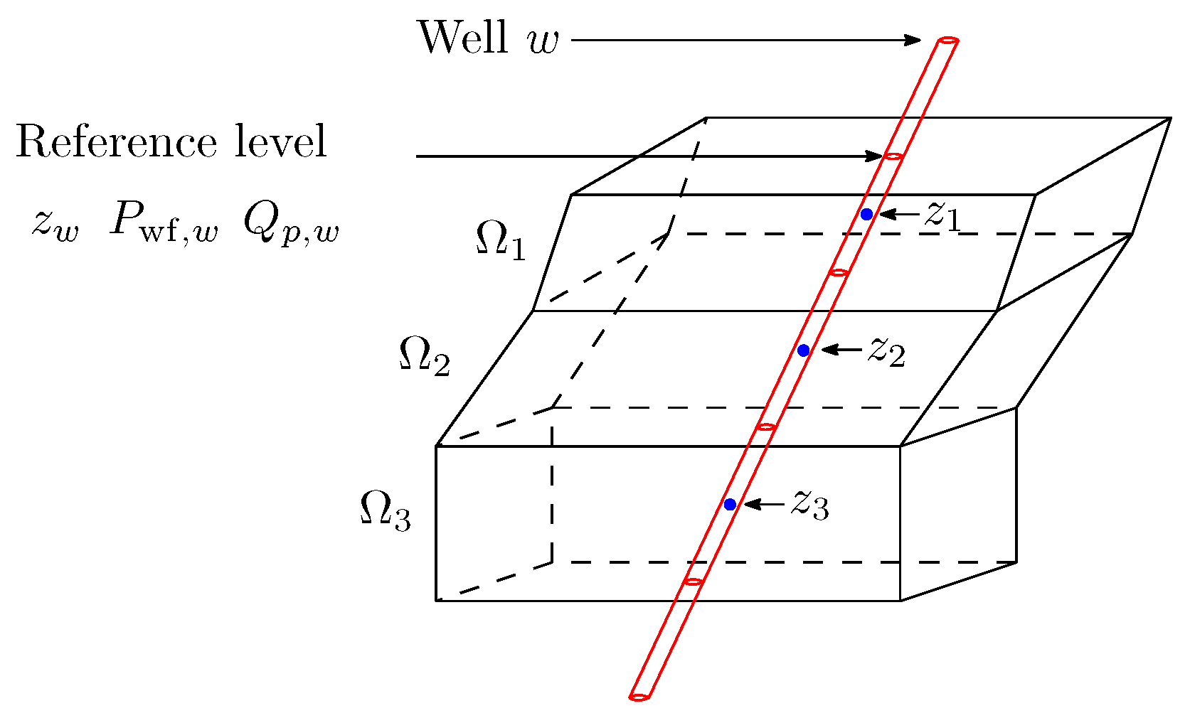
However, in engineering applications, an approach of type (34) is not practical in most cases, mainly because this term is used for including injection/production well modeling, implying the function is highly discontinuous on the domain. Additionally, component k can be produced in different phases and is associated with the volumetric rates of each phase , through the molar fraction . In this case, additional equations are required [76]. Peaceman extended well model [77] is used in this work. In this way, the source/sink term is thoroughly characterized as:
where is the bottom hole well pressure and is the well index upscaling factor of element defined as
The coefficient is the skin factor [78], which allows for considering permeability reductions in well-bore damage. The geometrical elements used here are shown schematically in Figure 2.
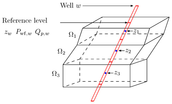
Figure 2.
Schematization of the geometric elements involved in the discretization of well model.
Also, it is worth mentioning that the variable is usually the determining variable for EOR economic models. For this reason, this variable is essential in the validation of the method (see numerical example Section 6.1).
Time Integration
For the time integrals, a generalized Crank Nicholson scheme [50], also known as implicit-explicit or IMEX method [51,52], is used. This scheme can be seen as a weighted trapezoidal rule [79] applied on a continuous function F as
where is the length of the time interval. The classical implicit and explicit schemes can be obtained directly by setting the parameter to 0 or 1, respectively. To simplify the notation, write .
4. Weighted Least Squares
4.1. General Formulation
Let a family of nodes in space, where is the index collection. Neglecting the truncation error, consider Taylor series centered at a point of interest which produces the following overdetermined system of linear equations obtained by evaluating for each :
where the number of nodes , are greater than the number of unknown partial derivatives until order m of the scalar function at . Moreover, the equation system (38) can be written in matrix form as
where is the number of unknowns. The weighted least squares [80,81] problem (WLS) for this formulation is: Find , approximated solution of (39), such that
where
Some authors take the p power equal to 1 or 2 [30,32,82].
WLS Solution
There are two equivalent alternatives to solve the WLS problems [83]. The first is to solve the linear system of normal equations , where the solution is given by:
where the matrix , is the Moore-Penrose weighted pseudo-inverse of , defined as:
The second alternative is to find an orthogonal projector , on the range of such that .
4.2. Stencil Definition
Depending on the selection of the point of interest , there are two possible definitions of the stencil for WLS application in a grid: cell stencils, where , and face stencils with .
4.2.1. Cell Stencils
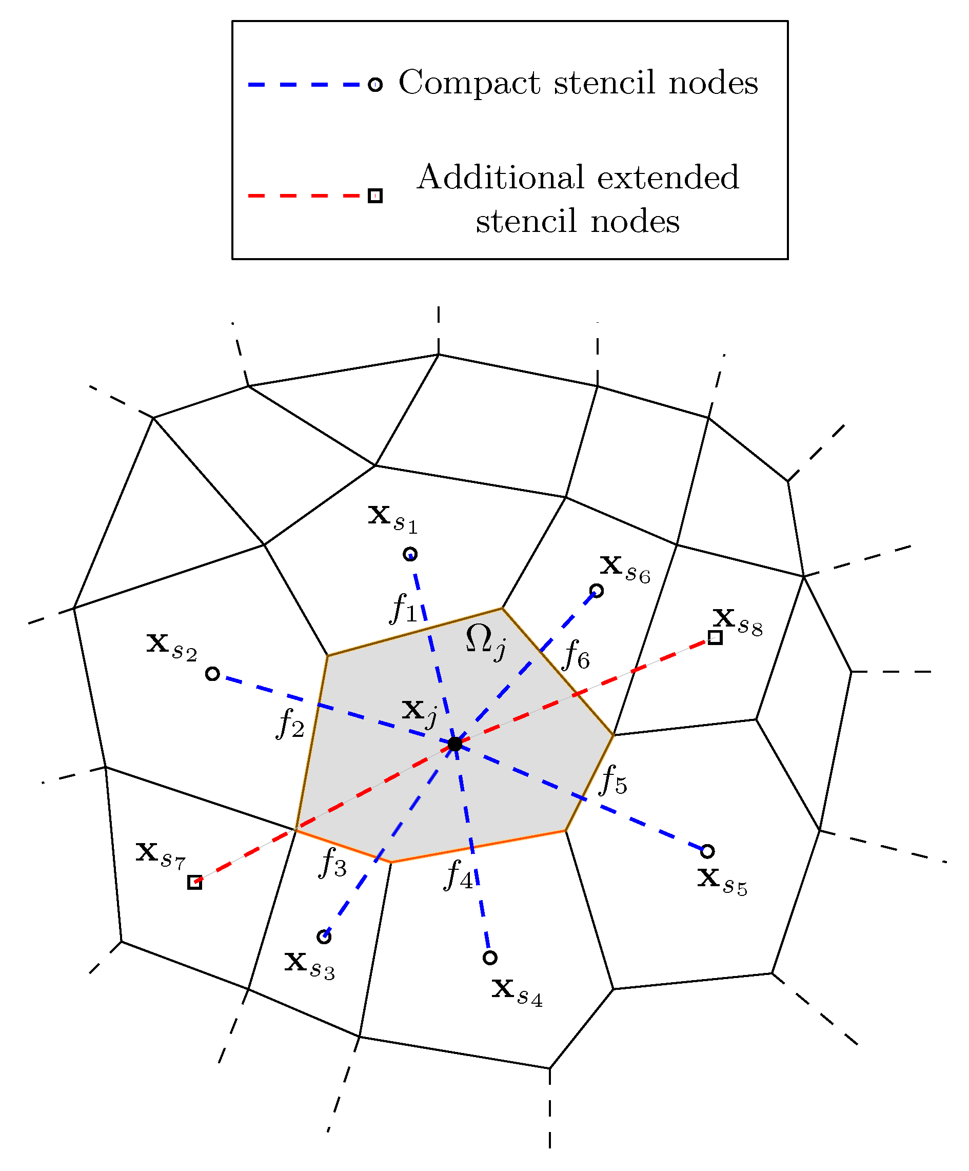
Let the set of nodes for stencil definition of an arbitrary cell . The most natural way to select these nodes is to take advantage of the connectivity of the cell through their faces, choosing the nodes of the neighboring elements, defining what is called a compact stencil [84]. Also, the stencil can be extended considering, not only the elements neighboring through the faces but those that have common nodes. For example, see Figure 3, in which the compact stencil is , and the extended stencil is given by .
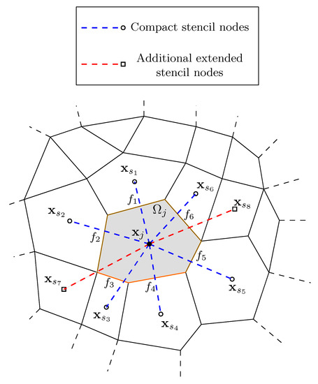
Figure 3.
Compact and extended cell stencils.
4.2.2. Face Stencils
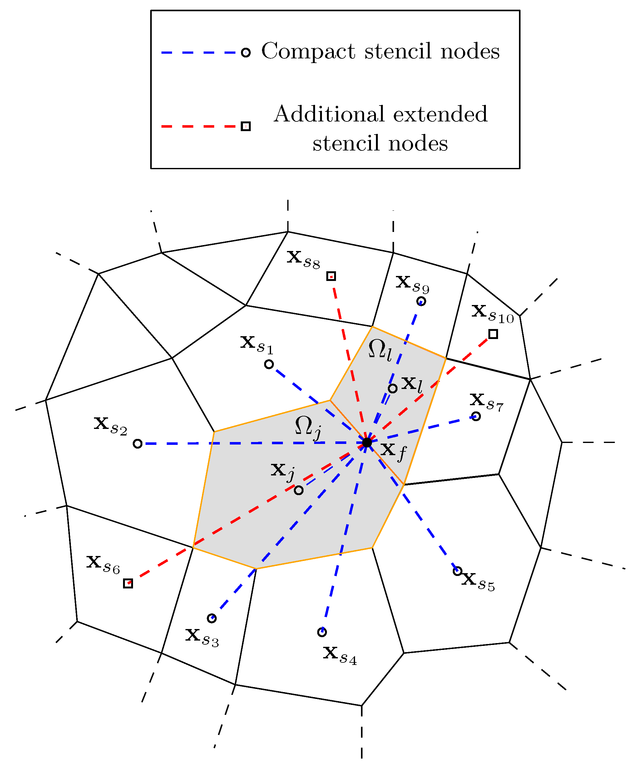
Let and nodes for either compact or extended stencils of neighboring cells and . The nodes for the face stencil are defined as
The typical definition of the face stencil is illustrated in Figure 4, in which .
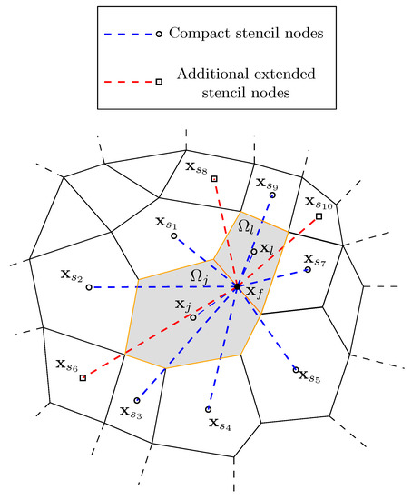
Figure 4.
Compact and extended face stencils.
This stencil construction, in terms of the connectivity of both cells, has its raison d’être; it guarantees a single stencil per face. This fact corrects a possible source of error in the formulation of Loudyi [32] in which the face stencil is relative to each cell. This source of error causes numerical instabilities in Newton’s method when solving the resultant algebraic system from finite volume discretization, mainly because of the difference between fluxes at each cell residual, which can lead to non-convergence when the algebraic equations system is ill-conditioned; a condition that is not unusual in the modeling of multiphase flow in porous media [85].
4.2.3. Stencils at Boundaries
If the point of interest lies in a boundary cell with Neumann or Dirichlet faces, then some information is known depending on its boundary type. This information allows for simplifying the overdetermined system (38) by adding the boundary face nodes to the stencil, as is shown schematically in Figure 5.
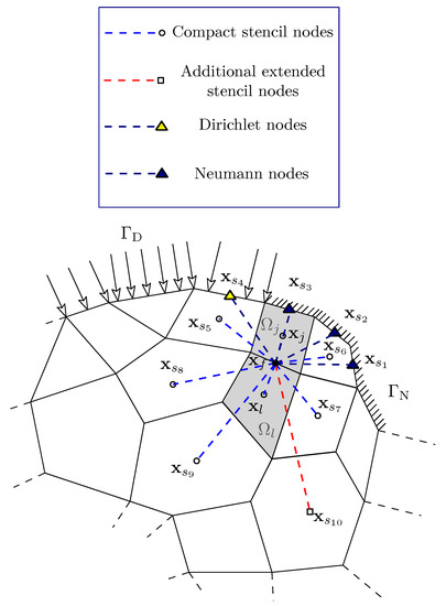
Figure 5.
Face stencils with boundary nodes.
4.3. Gradient Reconstruction
The application of (38) to approximate the gradient derivatives for the potential at time n, in the point of interest is
where the coefficients , , and are the components of the vector . It is essential to take account of the sign of each coefficient because it considers the orientation of the Taylor series radius. If a cell stencil is used, the procedure requires an additional interpolation [86,87] in order to obtain the gradient at the face required by (24). The most common way to do this is the linear interpolation between the gradient values at neighboring cell centroids, given by
where
In this case, to guarantee the second-order convergence when (46) is used, an additional correction for skewness is required [88,89].
4.4. Hessian Reconstruction
5. Semi-Implicit Implementation
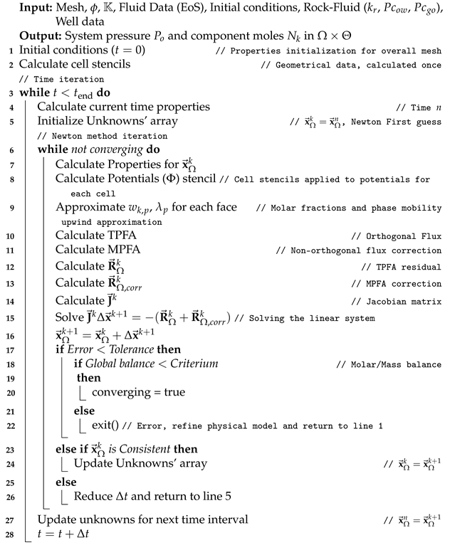
The formulation above is the guideline for FlowTraM semi-implicit implementation, which uses the Newton-Raphson method for algebraic equations linearization. This implementation is presented in Algorithm 1. The core steps in the algorithm, which allow for managing non-orthogonal geometries, are cell stencils and potential stencils calculation, required for multipoint flux approximation (MPFA); TPFA and MPFA calculation, and residual correction.
In cell stencil calculations, the matrix operator is created, which depends on its geometrical information, like , , . This process is done once per simulation unless changes exist in geometry through time. If absolute permeability remains constant, alpha and beta shape factors can be calculated to this stage.
Subsequently, in potential stencil calculations, gradients per cell are reconstructed by solving the overdetermined linear system given by cell-matrix operators and time k potentials . Later, face gradients are obtained via interpolation using the centroid distance between two neighboring cells. MPFA calculation refers to non-orthogonal flux calculation.
Finally, a correction for residual is obtained by accumulating non-orthogonal fluxes for each face of a cell. The resulting correction is added to residual in Newton iteration, and a corrected solution is obtained by applying a preconditioned iterative solver like GMRES with ILU to Newton’s linear system.
The proposal above is called semi-implicit because, for MPFA calculation in gradient reconstruction, time k potentials are used . Nonetheless, these fluxes are omitted in Jacobian matrix calculation but added as a correction to TPFA residual. It is worth noting that, with this approach, the sparse nature of the Jacobian matrix is maintained.
| Algorithm 1 Semi-Implicit approach Pseudocode |
 |
6. Numerical Experiments and Discussion
The proposed methodology was proven successful in Colciencias 273-2017, 272-2017, 064-2018 projects. These were aimed at the development of technologies for EOR processes, to maximize usages of oil reserves in Colombia, thus, demonstrating our model versatility. Nevertheless, in this work, three numerical experiments are presented. The first one is for validating the methodology; the second one presents a pseudo-compositional implementation to reproduce a Black-oil study case, and the third one is for demonstrating practical usage and applying it to a field case.
The first experiment is an adaptation of the Third Comparative Solution Project (SPE3) [90], simulated on a mesh with high non-orthogonalities. The obtained results allow for validating the formulation and help to illustrate the improvement when corrective fluxes are introduced clearly. The second numerical experiment is a three-phase conning study in a radial mesh, which is used to compare multiple commercial simulators and validate newer ones. The third experiment is a history matching of parameters for a Colombian oil field at the llanos basin, located at Piedemonte llanero, a realistic simulation.
6.1. SPE Comparative Solution Project 3
This simulation problem consists of a gas re-circulation, for pressure maintenance, in a heterogeneous reservoir of condensate gas. Dry gas is injected at 4.7 MMSCF/day in the upper area of the reservoir and sustained for ten years, while the lower area of the reservoir has a producing well conditioned to 6.2 MMSCF/day. Fluid properties are listed in Table 1.

Table 1.
Properties of condensate gas evaluated in the third SPE comparative project [90].
The orthogonal and the adapted non-orthogonal grids used to simulate this case are shown in Figure 6. Moreover, Figure 6 shows the cell average of the K-orthogonality angle, defined for each face by
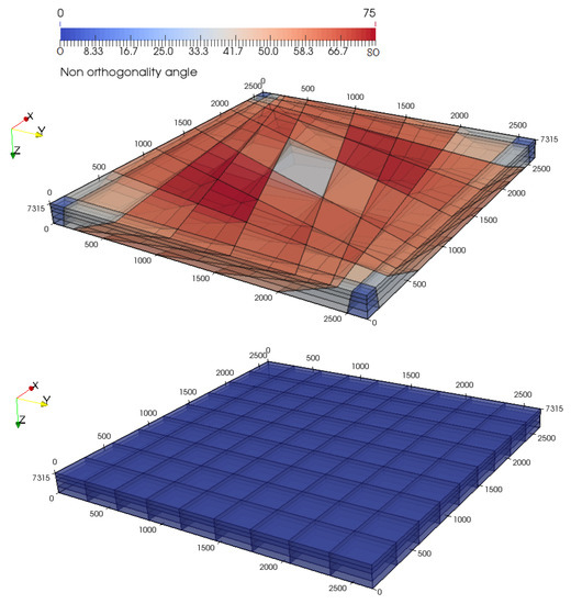
Figure 6.
SPE 3 adapted test geometries: Non-orthogonal (top) and reference orthogonal (bottom).
The pressure distribution for both geometries is presented in Figure 7 for different time steps. Due to the pressure drop caused during gas production, condensate oil banks continuously appear in the producing blocks. These banks become mobile when they reach critical saturation, which in this case, is 16%. Thus, once formed, they can only disappear by contact with very light gases or by an additional depressurization that causes the gradual volatilization of its lighter components.
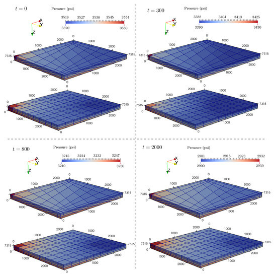
Figure 7.
Pressure variation at different time steps in both, orthogonal an non-orthogonal grid (fully corrected).
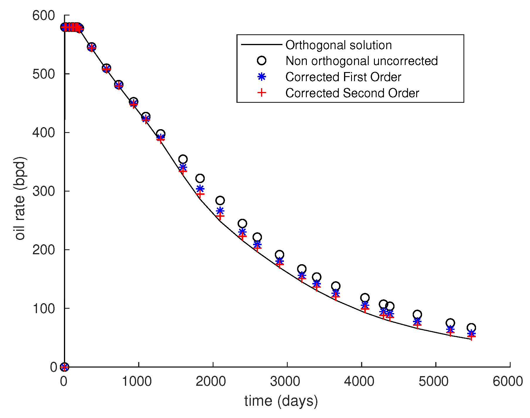
The oil produced in this reservoir is governed by condensation of intermediate components from the gas phase once it reaches the surface and oil mobilization once the critical saturation is reached. Notice that the most significant variable in reservoir simulation is the oil rate computed at the surface. Figure 8 shows surface oil production for the different test geometries. The obtained results validate the implemented formulation in FlowTraM and show the improvement in convergence obtained by introducing the proposed first and second-order corrective flows.
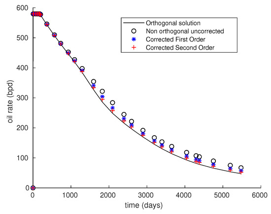
Figure 8.
Oil rate at surface computed in orthogonal and non-orthogonal geometries.
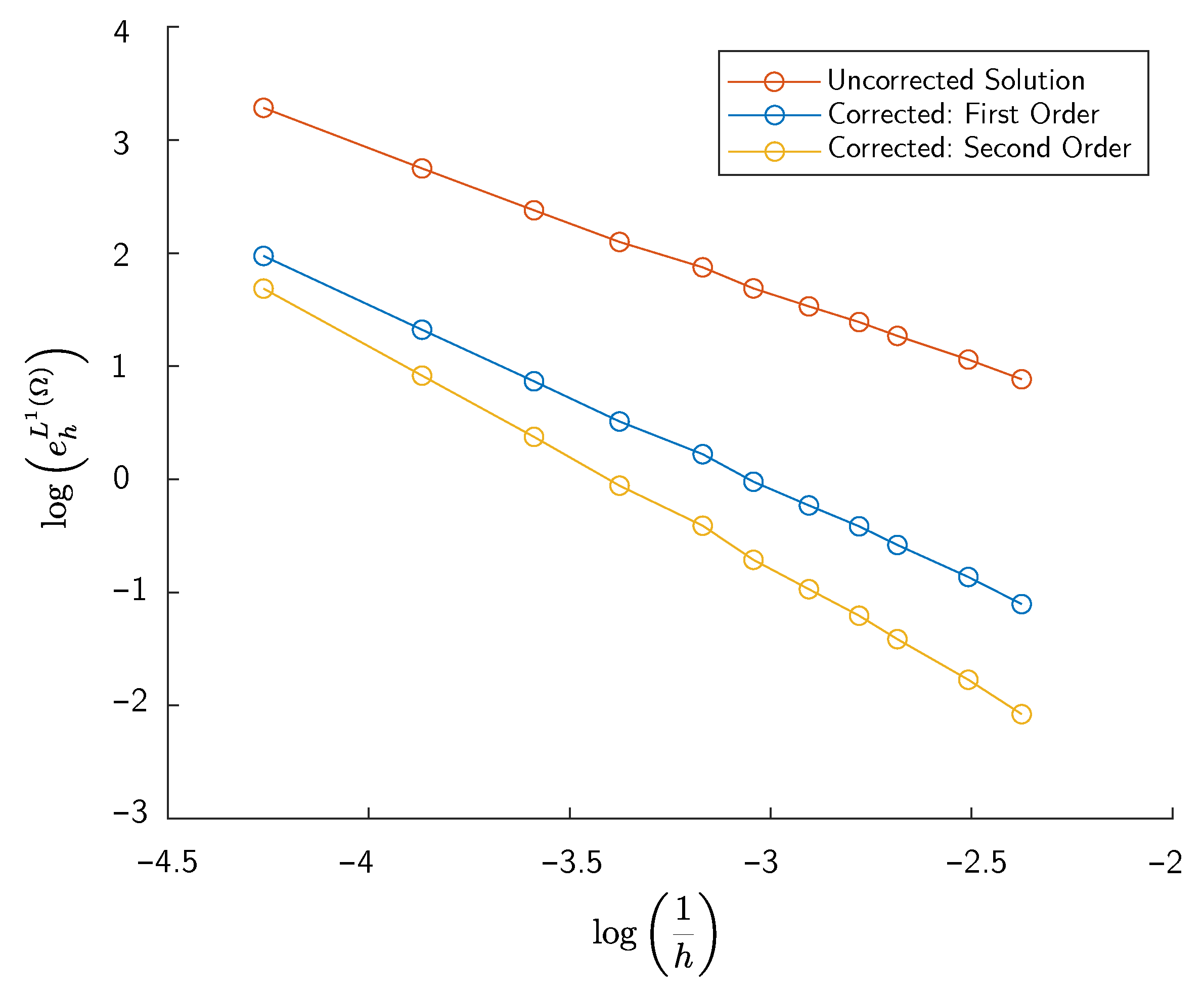
Convergence Analysis
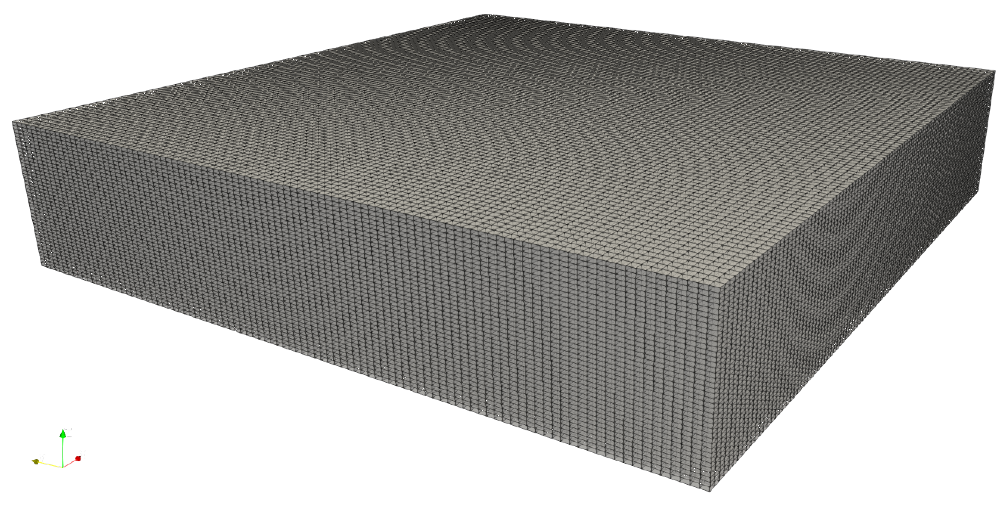
In order to validate the effect of the correction schemes, we performed a convergence analysis using a significantly refined orthogonal mesh geometry as a reference solution, in the absence of an analytical solution for this problem. The spatial discretization of the reference mesh is represented by , , , whose result is shown in Figure 9.
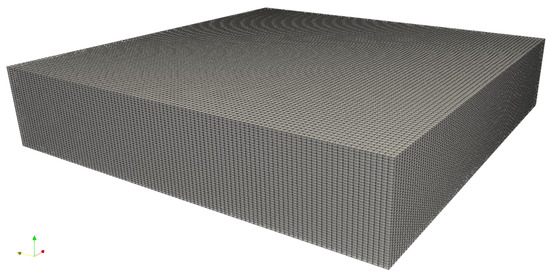
Figure 9.
Orthogonal mesh used to compute the reference solution.
The analysis makes use of the normalized experimental error in norm , defined as
where is the resolved potential in the reference mesh, and is the solution in a skewed non-orthogonal mesh of size h, which can be defined as
These meshes were constructed analogously to the one shown in Figure 6. The results are shown in Table 2, for which the order of convergence has been calculated as
Table 2.
Convergence analysis results (UC:Uncorrected; FOC:First Order Corrected; SOC: Second Order Corrected).
The error behavior is depicted in Figure 10, where the logarithmic scales were chosen strategically to represent the rate of convergence as the slope of the curves. These results prove the effectiveness of the corrective fluxes as expected, reducing the magnitude of the error and improving the rate of convergence with both first and second-order corrections. In each case, corrective fluxes recover the order of convergence previously lost due to the mesh non-orthogonality and skewness effects.
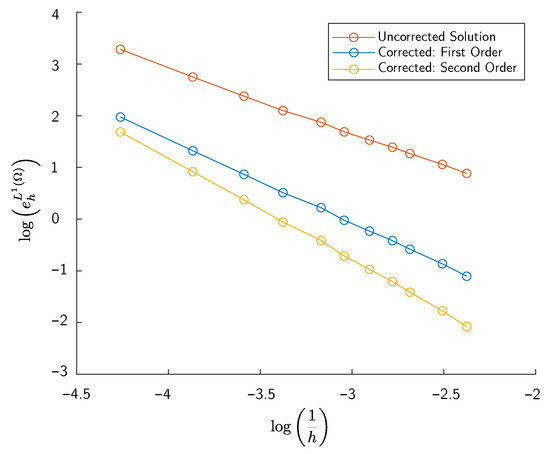
Figure 10.
Convergence analysis plot: is the slope at each curve interval.
6.2. SPE Comparative Solution Project 2
The SPE second comparative solution project (SCSP) is a coning study of three phases in a single-well radial cross-section with logarithmic distribution in the radial axis. This simulation case consists of one production well having step variations in the production rate, representing a numerical challenge, which serves for testing convergence and stability capabilities [91].
The thermodynamic behavior of the fluid studied in the SCSP is represented by Black Oil fluid model (see Table 3). Table 3 shows the densities , volumetric factors , viscosities (), and gas-oil ratio , as a function of the fluid pressure. Black Oil PVT data is converted into equilibrium relations, which serve for calculating thermodynamic state, i.e., components and phases composition, and gas and oil molar fractions in oleic and gaseous phases. FlowTraM uses this converted data for solving thermodynamic state, molar balance, and volume conservation equations in a pseudo-compositional model.
Table 3.
PVT Table for SCSP [91].
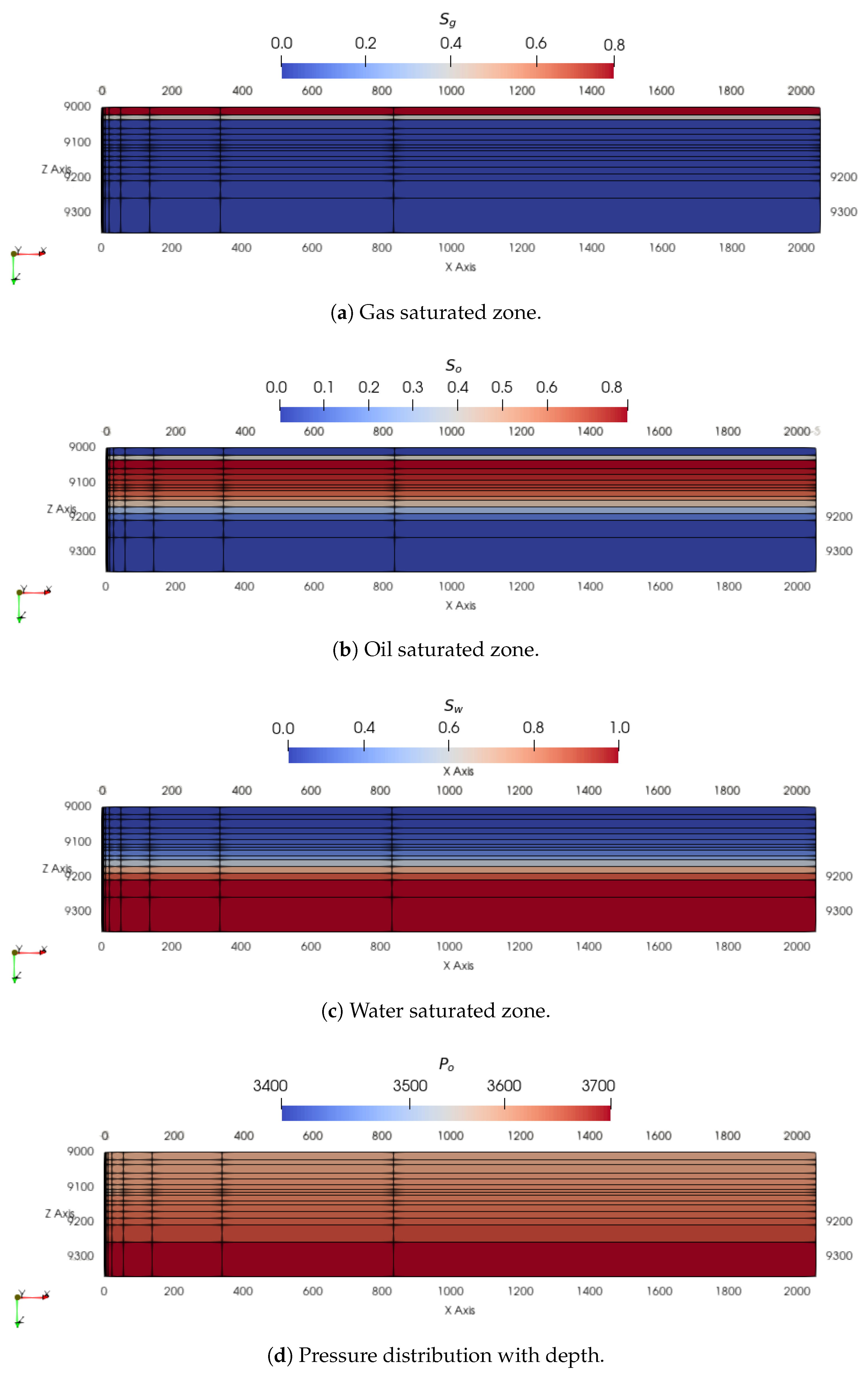
SCSP reservoir is initially at gravitational and capillary equilibrium conditions. Thus, fluids locate in specific zones, and pressure increases with depth. Figure 11a–c show gas, oil, and water saturation, respectively, with their transition zones. Additionally, pressure variation with depth is presented in Figure 11d.
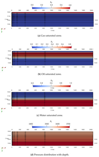
Figure 11.
Reservoir initial conditions , saturations and pressure distribution at gravitational and capillary equilibrium.
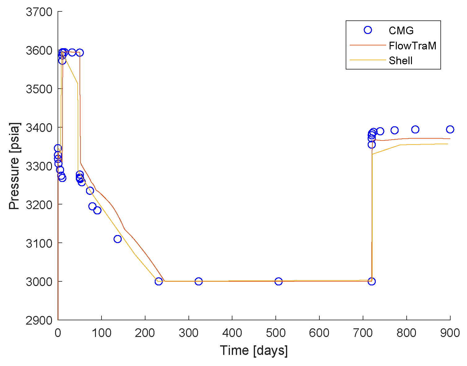
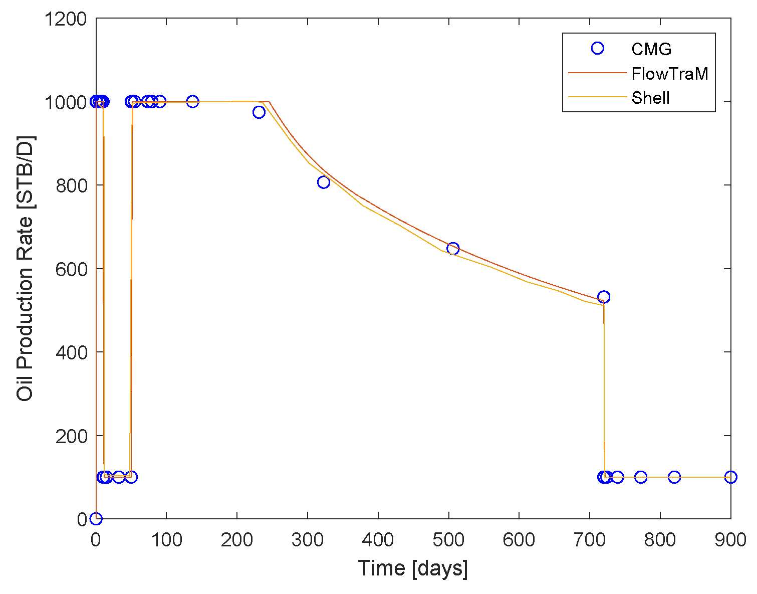
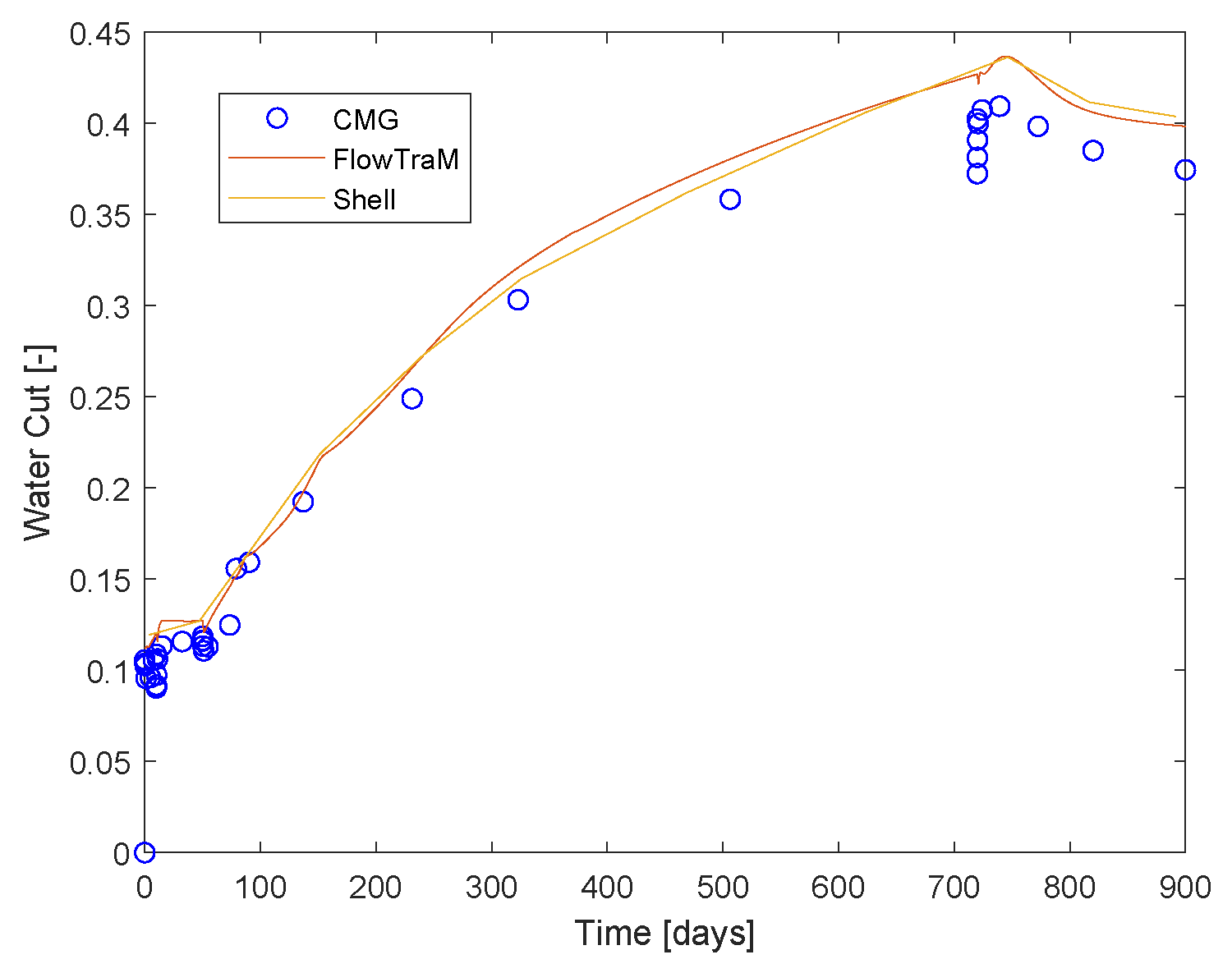
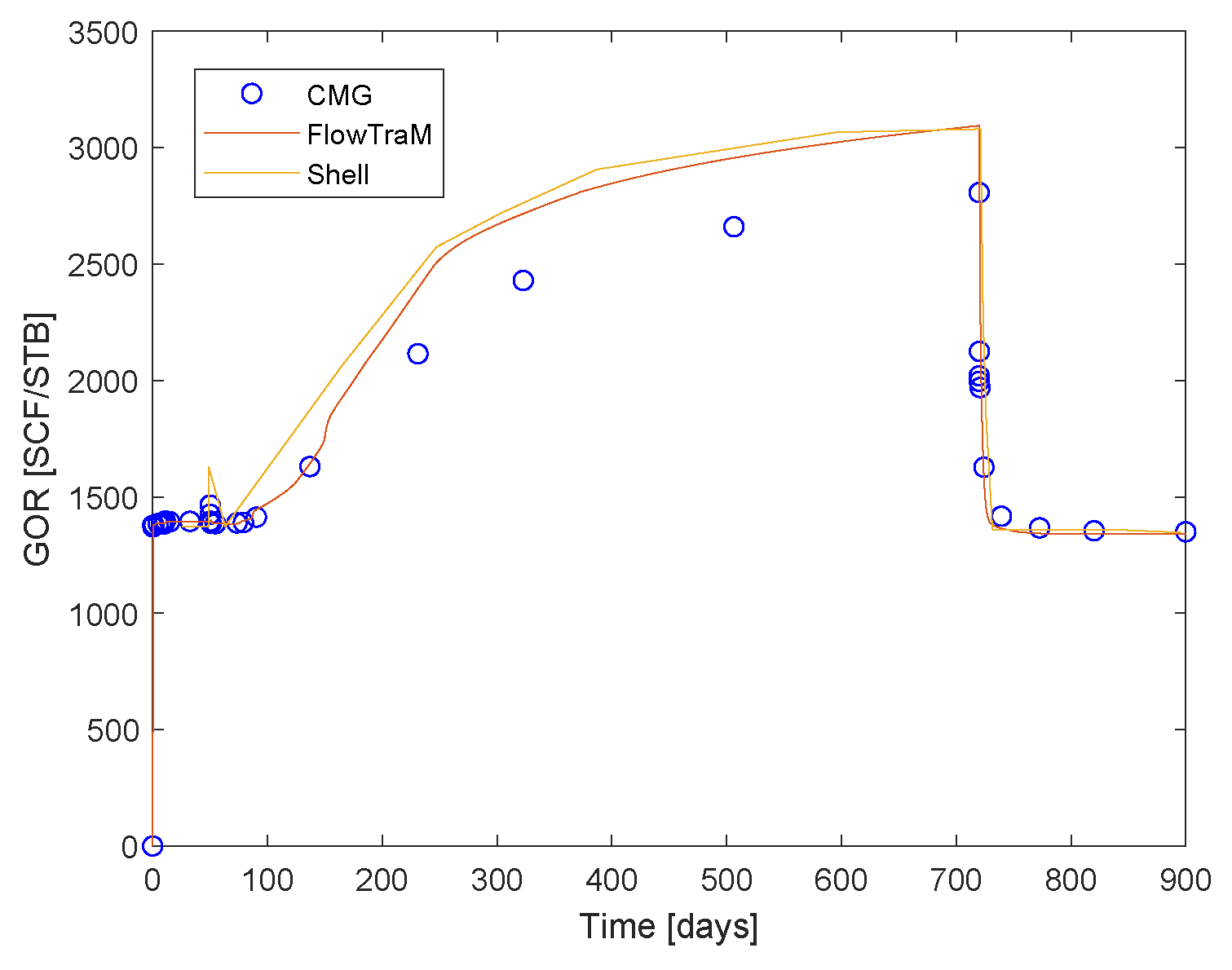
We compared FlowTraM simulation results with the predictions of CMG IMEX, which we obtained by running a pre-designed input file in CMG library; and with Shell simulator results, which we took from SCSP paper results [91]. Borehole pressure, oil rate production, and water cut at the production well are shown in Figure 12, Figure 13 and Figure 14, respectively. It is worth noting that both Shell, IMEX, and FlowTraM results are in accordance. Nonetheless, Gas-Oil ratio (GOR) results on FlowTraM, presented in Figure 15, are significantly higher than IMEX results. These results are due to physical model differences. However, FlowTraM GOR results fit better with Shell results. Furthermore, FlowTraM results approximate to the average between other simulators GOR reported in SCSP paper results [91].
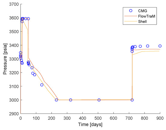
Figure 12.
Comparison of Borehole pressure at production well.
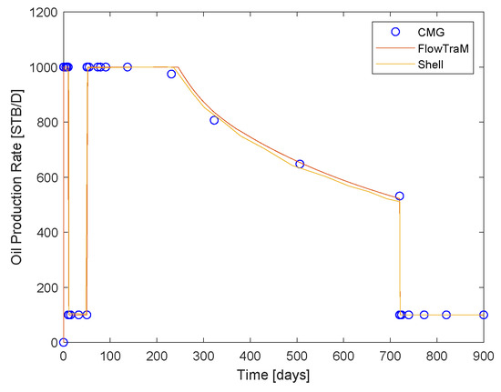
Figure 13.
Comparison of oil production rate.
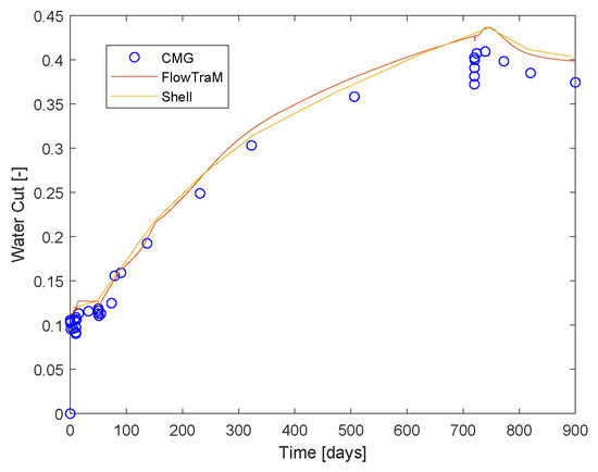
Figure 14.
Comparison of water cut.
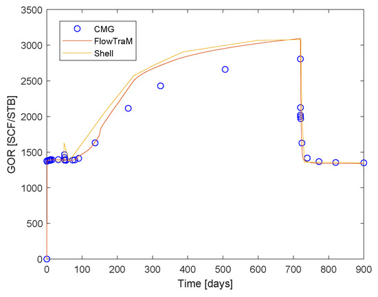
Figure 15.
Comparison of Gas oil ratio.
6.3. Colombian Volatile Oil Field Case
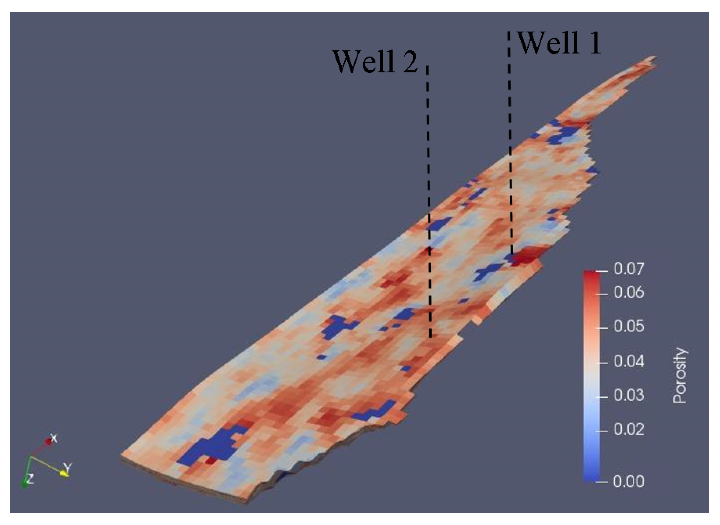
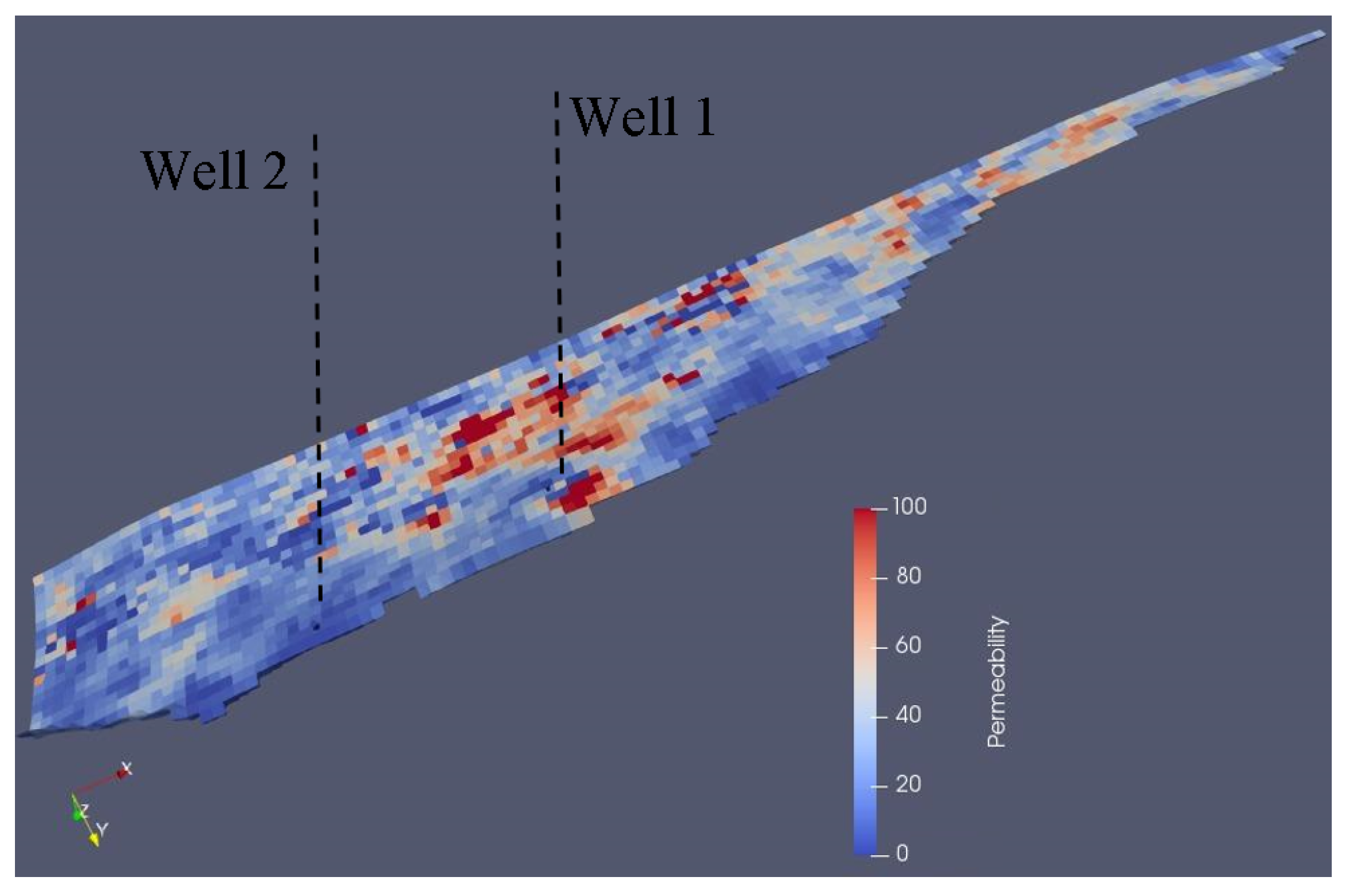
The field study case is a sector model of a volatile oil field in the Colombian foothills, Llanos basin. A heterogeneous simulation grid with 37,960 blocks was used to simulate the recovery process at a reservoir scale, with permeability changes between 1 and 100 mD and porosity between 1–6.7%. The mesh porosity and permeability distributions of an intermediate layer are shown in Figure 16 and Figure 17. The dynamic model was calibrated using a history matching process in FlowTraM. The vertical dashed lines represent production and injection wells.

Figure 16.
Field porosity distribution.

Figure 17.
Field permeability distribution.
Historical well information is the most sensitive information when making a history matching. The dynamic model must be able to reproduce the historical pressure or production data, depending on the operating condition imposed on it. That is, the simulator must reproduce the historical production if it is fed with the flowing well pressure, or reproduce the historical background pressure if it is fed with the production data. For the system evaluated in this work, the simulator is fed with background pressure data for producing wells (seeking to reproduce production) and with injection flow data for injection wells (seeking to reproduce background pressure).
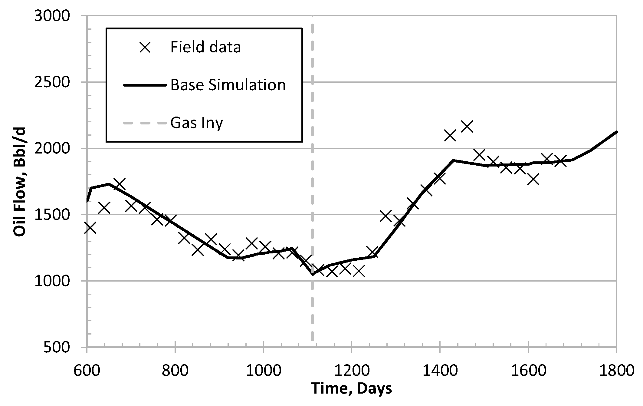
For initializing the simulation model, an initial pressure of 4500 psi is set at 12,000 ft. Initial water saturation is 0.22, and the average oil saturation is 0.78. The distance between wells is about 11,000 ft. Producing well is programmed to produce with an increasing bottom hole pressure from 3000 psi at the beginning, to 3500 psi at day 1110, then the well continues producing at a constant pressure of 3500 psi. The injector well is programmed to start injection with 45 MMSCF/day from day 1110.
For obtaining the history matching, the information supplied by an operator company was directly introduced into the flow simulator. The production was evaluated, taking into account the historical productivity and sensitivity of the flow correlation in pipes, aiming to obtain well constraints that fitted its productivity.
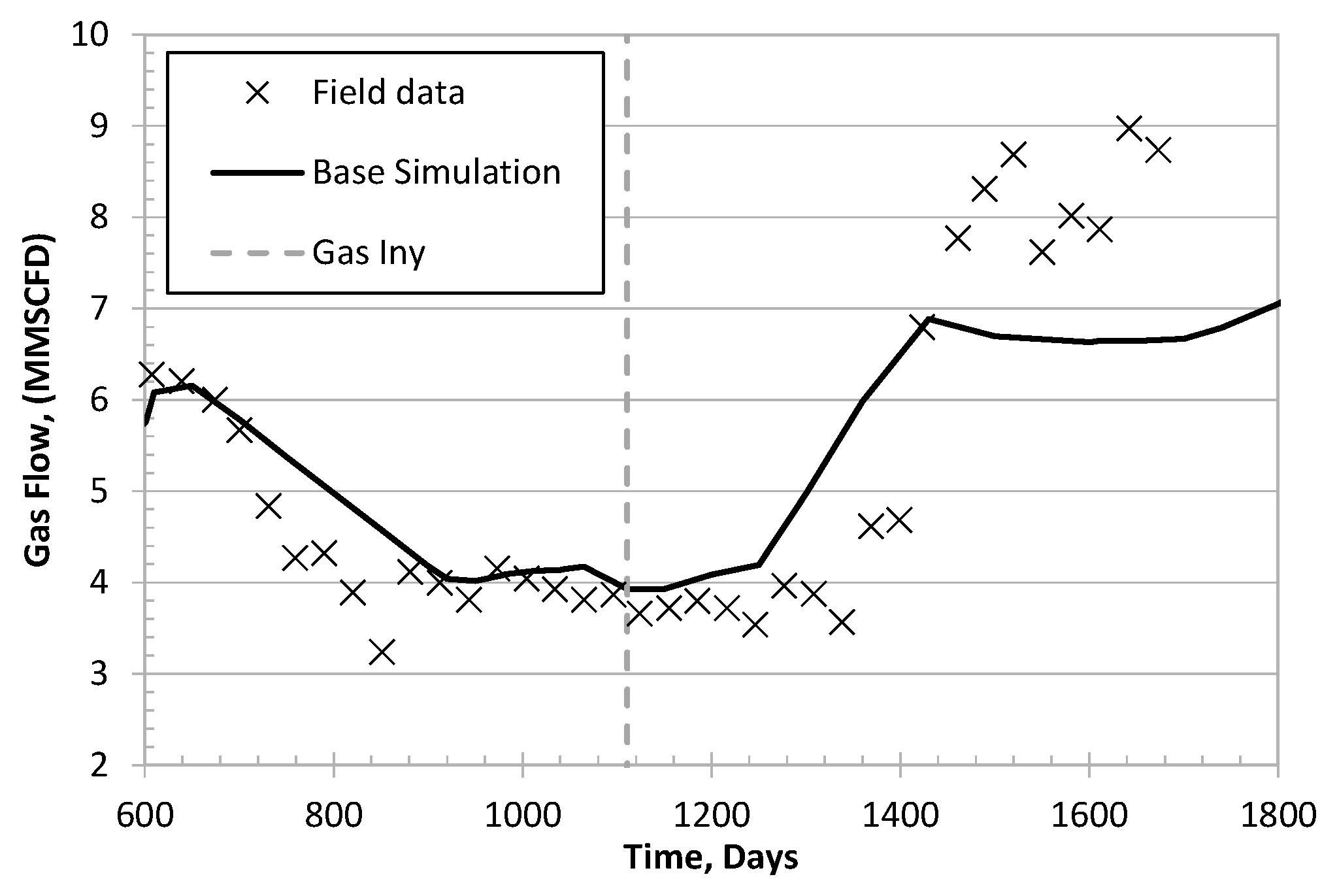
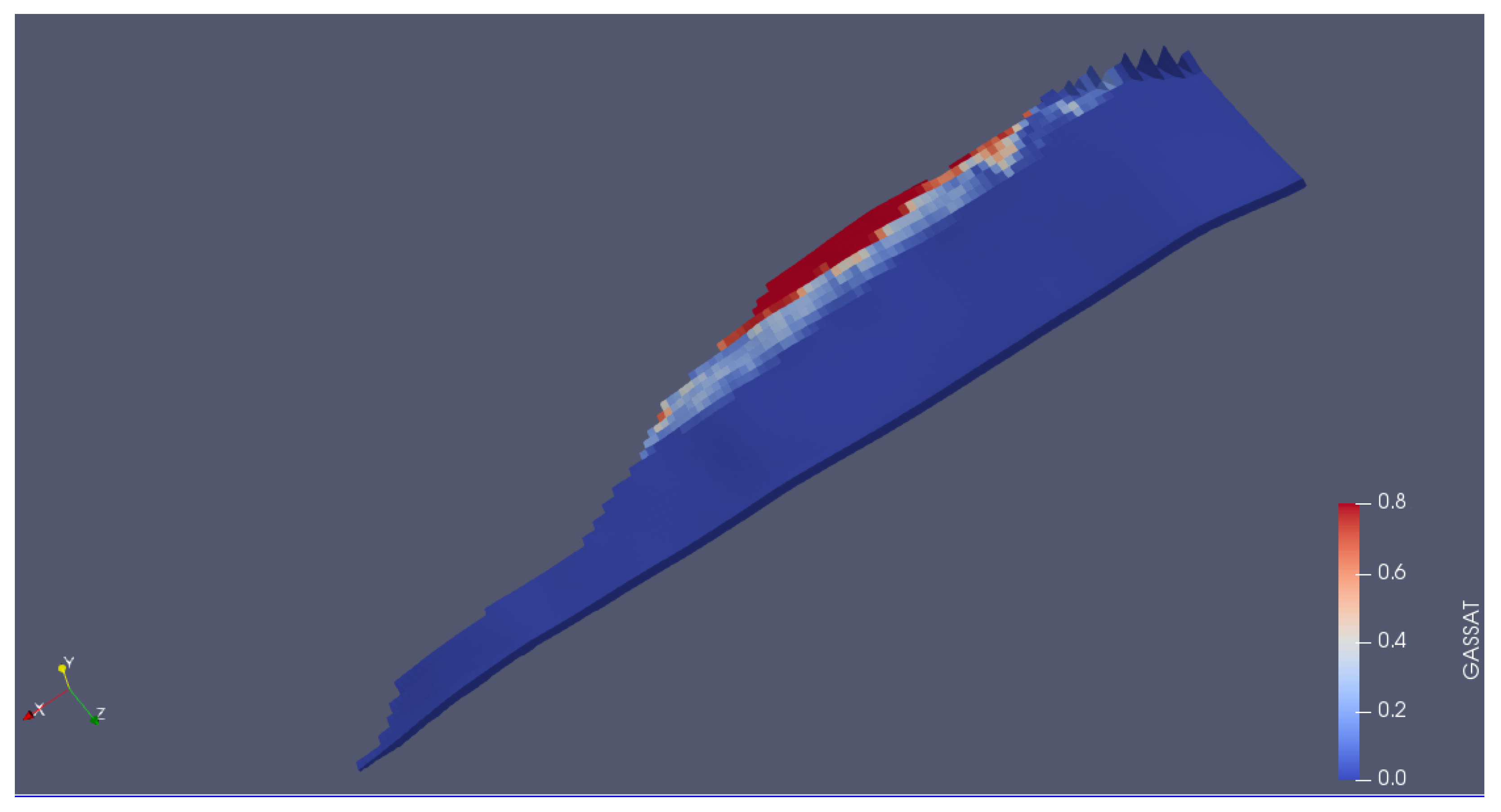
Oil and gas production are presented respectively in Figure 18 and Figure 19, where it is shown that the model can reproduce the effects of recycle gas injection and the production history of the reservoir. At a field scale, the simulation results showed a good agreement with field measurements. Also, the gas saturation distribution is presented in Figure 20.

Figure 18.
Oil production. Symbols: field measurements; continuous line: baseline.
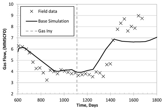
Figure 19.
Gas production. Symbols: field measurements; continuous line: baseline.

Figure 20.
Gas saturation distribution in the reservoir (day 1770).
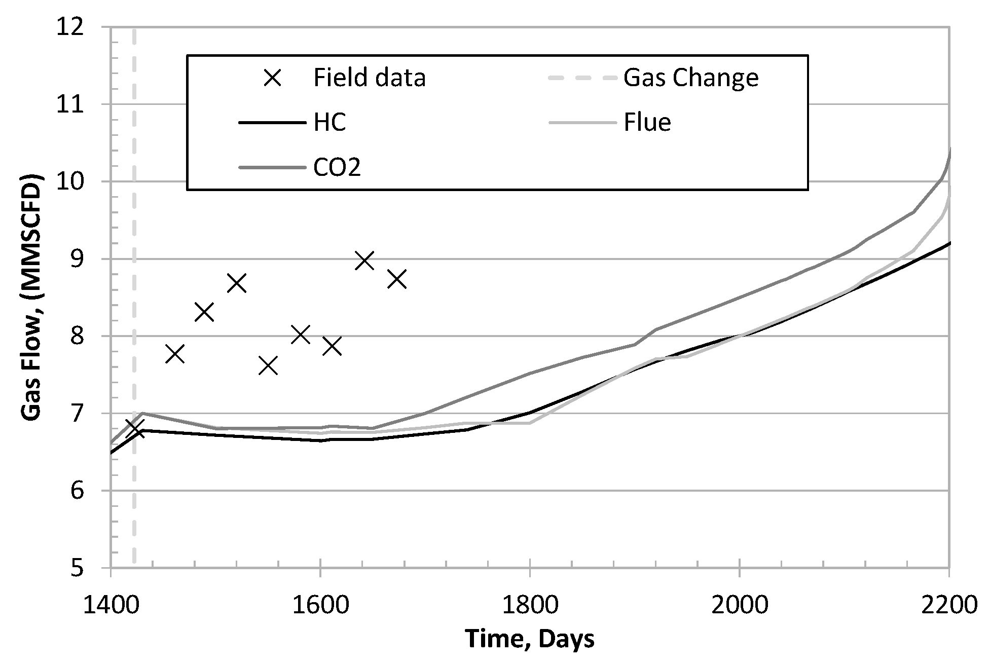
Once the historical matching has been verified, different gas injection is evaluated from day 1423: CO, Flue gas, and recycle gas at a fixed rate of 12 MMSCF/day. Figure 21 and Figure 22 show the simulation results for oil and gas, respectively, with the different injection gases, where it is observed that CO is the gas with the best productivity response.
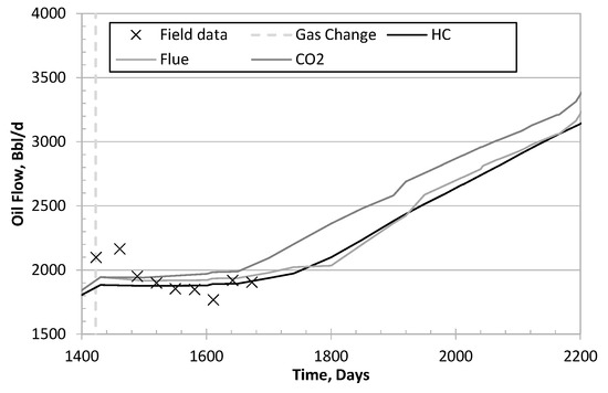
Figure 21.
Oil production after different gas injection. Symbols: field measurements; continuous line: baseline.
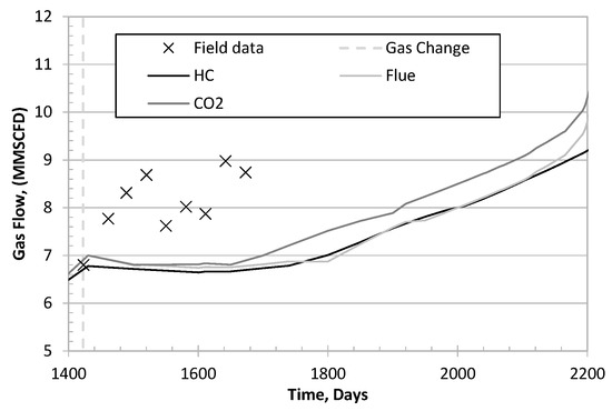
Figure 22.
Gas production after different gas injection. Symbols: field measurements; continuous line: baseline.
7. Conclusions and Future Work
This work serves as a basis for the construction of more robust numerical methods. The goal is to account for significant problems regarding flow in highly anisotropic and heterogeneous porous media, as in many applications in the oil industry, whose solutions benefit from conservative numerical methods. In this sense, a new version of the unstructured finite volume method is proposed, with an improved scheme of the traditional two-point flux approximation, allowing for dealing with the phenomenon of non-orthogonality of the meshes and the effect of the full permeability tensor. Additionally, a direct consequence of our formulation is the correction of errors due to the mesh skewness. Moreover, the mathematical formulation based on the second-order anisotropic elliptic operator allows the method to be applied in diverse engineering applications, like enhanced oil recovery, at a low cost. Furthermore, we proposed a modification to Newton’s method to efficiently apply the corrections, maintaining the sparse nature of the Jacobian matrix.
The comparisons done in several numerical examples, between FlowTraM, CMG-IMEX, and Shell simulator, demonstrate that our results follow other commercial simulators’. In the specific case of SCSP, our approximation to Gas-Oil ratio is closer to the average between GOR values reported by other simulators in SCSP paper results [91]. Moreover, on a Colombian field history-matching, we present the capability of FlowTraM for reproducing an actual field operation.
The next stage of this work is to analyze and to compare the performance of the UFVM here presented with respect to the variational methods as DG and FEM. The current development and implementation of UFVM are planned to be extended to chemical transport and thermal recovery applications. Also, more elaborate models can be included for unconventional wells [92] and elements of any geometries [93] in the source/sink term discrete equations.
Author Contributions
Conceptualization, S.E.-M., S.V., N.B., J.D.V. and H.A.S.; Data curation, S.E.-M. and S.V.; Formal analysis, S.E.-M.; Funding acquisition, H.A.S., J.M.M. and J.D.V.; Investigation, S.E.-M., S.V., N.B. and J.D.V.; Methodology, S.E.-M., S.V. and N.B.; Project administration, J.M.M.; Software, S.E.-M., S.V., N.B. and J.D.V.; Supervision, J.M.M.; Validation, S.E.-M., S.V., N.B., J.D.V. and H.A.S.; Visualization, S.E.-M., S.V. and J.D.V.; Writing—original draft, S.E.-M., S.V., N.B. and J.D.V.; Writing—review & editing, S.E.-M., S.V., N.B. and J.D.V. All authors have read and agreed to the published version of the manuscript.
Funding
This research was funded by FONDO NACIONAL DE FINANCIAMIENTO PARA LA CIENCIA, LA TECNOLOGÍA Y LA INNOVACIÓN FRANCISCO JOSÉ DE CALDAS, MINCIENCIAS, Agencia Nacional de Hidrocarburos (ANH), and Universidad Nacional de Colombia under the agreements 273-2017, 064-2018, and 272-2017.
Institutional Review Board Statement
Not applicable.
Informed Consent Statement
Not applicable.
Acknowledgments
Authors thank Universidad Nacional de Colombia for logistic and financial support, and the research group Flow and Transport Dynamics in porous media for their contributions on this work.
Conflicts of Interest
The funders had no role in the design of the study; in the collection, analyses, or interpretation of data; in the writing of the manuscript, or in the decision to publish the results.
References
- Weller, H.G.; Tabor, G.; Jasak, H.; Fureby, C. A tensorial approach to computational continuum mechanics using object-oriented techniques. Comput. Phys. 1998, 12, 620–631. [Google Scholar] [CrossRef]
- Delshad, M.; Pope, G.; Sepehrnoori, K. A compositional simulator for modeling surfactant enhanced aquifer remediation, 1 formulation. J. Contam. Hydrol. 1996, 23, 303–327. [Google Scholar] [CrossRef]
- Neuman, S.P. Saturated-unsaturated seepage by finite elements. J. Hydraul. Div. 1973, 99, 2233–2250. [Google Scholar] [CrossRef]
- Cheah, E.P.; Reible, D.D.; Valsaraj, K.T.; Constant, W.; Walsh, B.W.; Thibodeaux, L.J. Simulation of soil washing with surfactants. J. Hazard. Mater. 1998, 59, 107–122. [Google Scholar] [CrossRef]
- Corapcioglu, M.Y.; Baehr, A.L. A compositional multiphase model for groundwater contamination by petroleum products: 1. Theoretical considerations. Water Resour. Res. 1987, 23, 191–200. [Google Scholar] [CrossRef]
- Singh, A.; Delfs, J.O.; Böttcher, N.; Taron, J.; Wang, W.; Görke, U.J.; Kolditz, O. A Benchmark Study on Non-isothermal Compositional Fluid Flow. Energy Procedia 2013, 37, 3901–3910. [Google Scholar] [CrossRef] [Green Version]
- Correia, N.; Robitaille, F.; Long, A.; Rudd, C.; Šimáček, P.; Advani, S. Analysis of the vacuum infusion moulding process: I. Analytical formulation. Compos. Part A Appl. Sci. Manuf. 2005, 36, 1645–1656. [Google Scholar] [CrossRef]
- Michaud, V.; Mortensen, A. Infiltration processing of fibre reinforced composites: Governing phenomena. Compos. Part A Appl. Sci. Manuf. 2001, 32, 981–996. [Google Scholar] [CrossRef]
- Valencia, J.D.; Ocampo, A.; Mejía, J.M. Development and Validation of a New Model for In Situ Foam Generation Using Foamer Droplets Injection. Transp. Porous Media 2018, 131, 251–268. [Google Scholar] [CrossRef]
- Solano, H.; Valencia, J.; Mejía, J.; Ocampo, A. A Modeling Study for Foam Generation for EOR Applications in Naturally Fractured Reservoirs Using Disperse Surfactant in the Gas Stream. In Proceedings of the IOR 2019—20th European Symposium on Improved Oil Recovery, Pau, France, 8–11 April 2019. [Google Scholar]
- Pope, G.A.; Nelson, R.C. A chemical flooding compositional simulator. Soc. Pet. Eng. J. 1978, 18, 339–354. [Google Scholar] [CrossRef]
- Mohammadi, H.; Delshad, M.; Pope, G.A. Mechanistic modeling of alkaline/surfactant/polymer floods. SPE Reserv. Eval. Eng. 2009, 12, 518–527. [Google Scholar] [CrossRef]
- Bueno, N.; Mejía, J.M. Heavy oil in-situ upgrading evaluation by a laboratory-calibrated EoS-based reservoir simulator. J. Pet. Sci. Eng. 2020, 196, 107455. [Google Scholar] [CrossRef]
- Qin, X.; Wang, P.; Sepehrnoori, K.; Pope, G.A. Modeling asphaltene precipitation in reservoir simulation. Ind. Eng. Chem. Res. 2000, 39, 2644–2654. [Google Scholar] [CrossRef]
- Fazelipour, W.; Pope, G.A.; Sepehrnoori, K. Development of a fully implicit, parallel, EOS compositional simulator to model asphaltene precipitation in petroleum reservoirs. In Proceedings of the SPE Annual Technical Conference and Exhibition. Society of Petroleum Engineers, Denver, CO, USA, 21–24 September 2008. [Google Scholar]
- Darabi, H. Development of a Non-Isothermal Compositional Reservoir Simulator to Model Asphaltene Precipitation, Flocculation, and Deposition and Remediation. Ph.D. Thesis, The University of Texas at Austin, Austin, TX, USA, 2014. [Google Scholar]
- Darabi, H.; Sepehrnoori, K. Modeling and Simulation of Near-Wellbore Asphaltene Remediation Using Asphaltene Dispersants. In Proceedings of the SPE Reservoir Simulation Symposium, Society of Petroleum Engineersr, Houston, TX, USA, 21–23 February 2015. [Google Scholar]
- Eymard, R.; Gallouët, T.; Herbin, R. Finite volume methods. In Solution of Equation in Rn (Part 3), Techniques of Scientific Computing (Part 3), Handbook of Numerical Analysis; Elsevier: Amsterdam, The Netherlands, 2000; Volume 7, pp. 713–1018. [Google Scholar] [CrossRef] [Green Version]
- Versteeg, H.K.; Malalasekera, W. An Introduction to Computational Fluid Dynamics: The Finite Volume Method; Pearson Education: London, UK, 2007. [Google Scholar]
- Kocberber, S. An automatic, unstructured control volume generation system for geologically complex reservoirs. In Proceedings of the SPE Reservoir Simulation Symposium. Society of Petroleum Engineers, Dallas, TX, USA, 8–11 June 1997. [Google Scholar]
- Ponting, D.K. Corner point geometry in reservoir simulation. In Proceedings of the ECMOR I-1st European Conference on the Mathematics of Oil Recovery, Cambridge, UK, 14–16 July 1989. [Google Scholar]
- Ding, Y.; Lemonnier, P. Use of corner point geometry in reservoir simulation. In Proceedings of the International Meeting on Petroleum Engineering. Society of Petroleum Engineers, Beijing, China, 14–17 November 1995. [Google Scholar]
- LeVeque, R.J. Finite Volume Methods for Hyperbolic Problems; Cambridge University Press: Cambridge, UK, 2002; Volume 31. [Google Scholar]
- Lie, K.A.; Krogstad, S.; Ligaarden, I.S.; Natvig, J.R.; Nilsen, H.M.; Skaflestad, B. Open-source MATLAB implementation of consistent discretisations on complex grids. Comput. Geosci. 2012, 16, 297–322. [Google Scholar] [CrossRef] [Green Version]
- Georgoulis, E.H.; Hall, E.; Houston, P. Discontinuous Galerkin Methods on hp-Anisotropic Meshes I: A Priori Error Analysis. 2006. Available online: https://www.researchgate.net/publication/28692961_Discontinuous_Galerkin_Methods_on_hp-Anisotropic_Meshes_I_A_Priori_Error_Analysis (accessed on 13 September 2021).
- Formaggia, L.; Perotto, S. Anisotropic error estimates for elliptic problems. Numer. Math. 2003, 94, 67–92. [Google Scholar] [CrossRef]
- Arbogast, T.; Wheeler, M.; Yotov, I. Mixed Finite Elements for Elliptic Problems with Tensor Coefficients as Cell-Centered Finite Differences. SIAM J. Numer. Anal. 1997, 34, 828–852. [Google Scholar] [CrossRef] [Green Version]
- Cai, Z.; Jones, J.; McCormick, S.; Russell, T. Control-volume mixed finite element methods. Comput. Geosci. 1997, 1, 289–315. [Google Scholar] [CrossRef]
- Faille, I. A control volume method to solve an elliptic equation on a two-dimensional irregular mesh. Comput. Methods Appl. Mech. Eng. 1992, 100, 275–290. [Google Scholar] [CrossRef]
- Pasdunkorale, A.J.; Turner, I.W. A second order finite volume technique for simulating transport in anisotropic media. Int. J. Numer. Methods Heat Fluid Flow 2003, 13, 31–56. [Google Scholar] [CrossRef] [Green Version]
- Jayantha, A.; Turner, P.I.W. A comparison of gradient approximations for use in finite-volume computational models for two-dimensional diffusion equations. Numer. Heat Transf. Part B Fundam. 2001, 40, 367–390. [Google Scholar] [CrossRef] [Green Version]
- Loudyi, D.; Falconer, R.; Lin, B. Mathematical development and verification of a non-orthogonal finite volume model for groundwater flow applications. Adv. Water Resour. 2007, 30, 29–42. [Google Scholar] [CrossRef]
- Klausen, R.A.; Russell, T.F. Relationships among some locally conservative discretization methods which handle discontinuous coefficients. Comput. Geosci. 2004, 8, 341–377. [Google Scholar] [CrossRef]
- Pettersen, Ø. Basics of reservoir simulation with the ECLIPSE reservoir simulator. In Lecture Notes; University of Bergen: Bergen, Norway, 2006; p. 114. [Google Scholar]
- C.M.G. GEM CMG User Guide; Computer Modelling Group Ltd.: Calgary, AB, Canada, 2019. [Google Scholar]
- C.M.G. Advanced Process and Thermal Reservoir Simulator CMG STARS; Computer Modelling Group Ltd.: Calgary, AB, Canada, 2009. [Google Scholar]
- Zyvoloski, G.A.; Robinson, B.A.; Dash, Z.V.; Trease, L.L. User’s Manual for the FEHM Application-A Finite-Element Heat-and Mass-Transfer Code. 1997. Available online: https://www.osti.gov/biblio/14902-user-manual-fehm-application-finite-element-heat-mass-transfer-code (accessed on 13 September 2021).
- Kolditz, O.; Bauer, S.; Bilke, L.; Böttcher, N.; Delfs, J.O.; Fischer, T.; Görke, U.J.; Kalbacher, T.; Kosakowski, G.; McDermott, C.I.; et al. OpenGeoSys: An open-source initiative for numerical simulation of thermo-hydro-mechanical/chemical (THM/C) processes in porous media. Environ. Earth Sci. 2012, 67, 589–599. [Google Scholar] [CrossRef]
- Giammarco, P.D.; Todini, E.; Lamberti, P. A conservative finite elements approach to overland flow: The control volume finite element formulation. J. Hydrol. 1996, 175, 267–291. [Google Scholar] [CrossRef]
- Cao, H. Development of Techniques for General Purpose Simulators. Ph.D. Thesis, Stanford University, Stanford, CA, USA, 2002. [Google Scholar]
- Jiang, Y. Techniques for Modeling Complex Reservoirs and Advanced Wells. Ph.D. Thesis, Stanford University, Stanford, CA, USA, 2008. [Google Scholar]
- Wheeler, J. Integrated Parallel and Accurate Reservoir Simulator User’s Manual; Center for Subsurface Modeling, The University of Texas at Austin: Austin, TX, USA, 2007. [Google Scholar]
- Flemisch, B.; Darcis, M.; Erbertseder, K.; Faigle, B.; Lauser, A.; Mosthaf, K.; Müthing, S.; Nuske, P.; Tatomir, A.; Wolff, M.; et al. DuMux: DUNE for multi-phase, component, scale, physics, … flow and transport in porous media. Adv. Water Resour. 2011, 34, 1102–1112, New Computational Methods and Software Tools. [Google Scholar] [CrossRef]
- Bastian, P.; Blatt, M.; Dedner, A.; Engwer, C.; Klöfkorn, R.; Ohlberger, M.; Sander, O. A generic grid interface for parallel and adaptive scientific computing. Part I: Abstract framework. Computing 2008, 82, 103–119. [Google Scholar] [CrossRef]
- Bastian, P.; Blatt, M.; Dedner, A.; Engwer, C.; Klöfkorn, R.; Kornhuber, R.; Ohlberger, M.; Sander, O. A generic grid interface for parallel and adaptive scientific computing. Part II: Implementation and tests in DUNE. Computing 2008, 82, 121–138. [Google Scholar] [CrossRef]
- Baxendale, D.; Skaflestad, B.; Rasmussen, A.; Hove, J.; Rustad, A.B.; Lauser, A.; Skille, T.; Bao, K.; Sandve, T.H.; Blatt, M.; et al. OPEN POROUS MEDIA: Flow Documentation Manual; Equinox International Petroleum Consultants Pte. Ltd.: Tokyo, Japan, 2019. [Google Scholar]
- Lie, K.A. An Introduction to Reservoir Simulation Using MATLAB/GNU Octave: User Guide for the MATLAB Reservoir Simulation Toolbox (MRST); Cambridge University Press: Cambridge, UK, 2019. [Google Scholar] [CrossRef] [Green Version]
- Krogstad, S.; Lie, K.A.; Møyner, O.; Nilsen, H.M.; Raynaud, X.; Skaflestad, B. MRST-AD—An open-source framework for rapid prototyping and evaluation of reservoir simulation problems. In Proceedings of the SPE Reservoir Simulation Symposium. Society of Petroleum Engineers, Houston, TX, USA, 23–25 February 2015. [Google Scholar]
- Juretić, F.; Gosman, A.D. Error Analysis of the Finite-Volume Method with Respect to Mesh Type. Numer. Heat Transf. Part B Fundam. 2010, 57, 414–439. [Google Scholar] [CrossRef]
- Au, A.D.; Behie, G.; Rubin, B.; Vinsome, P. Techniques for fully implicit reservoir simulation. In Proceedings of the SPE Annual Technical Conference and Exhibition. Society of Petroleum Engineers, San Antonio, TX, USA, 8–11 October 1980. [Google Scholar]
- Ascher, U.M.; Ruuth, S.J.; Wetton, B.T. Implicit-explicit methods for time-dependent partial differential equations. SIAM J. Numer. Anal. 1995, 32, 797–823. [Google Scholar] [CrossRef]
- Rodrigues, S.B. Improving the IMEX method with a residual balanced decomposition. arXiv 2017, arXiv:1705.04870. [Google Scholar]
- Di Castro, A. Elliptic Problems for Some Anisotropic Operators. Ph.D. Thesis, University of Rome “Sapienza”, Rome, Italy, 2009. [Google Scholar]
- Mihăilescu, M.; Pucci, P.; Rădulescu, V. Eigenvalue problems for anisotropic quasilinear elliptic equations with variable exponent. J. Math. Anal. Appl. 2008, 340, 687–698. [Google Scholar] [CrossRef] [Green Version]
- Civan, F. Porous Media Transport Phenomena; John Wiley & Sons: Hoboken, NJ, USA, 2011. [Google Scholar]
- Bird, R.B.; Stewart, W.E.; Lightfoot, E.N. Transport Phenomena, 2nd ed.; John Wiley & Sons: New York, NY, USA, 2007. [Google Scholar]
- Bear, J. Dynamics of Fluids in Porous Media; Courier Corporation: North Chelmsford, MA, USA, 2013. [Google Scholar]
- Nield, D.A.; Bejan, A. Convection in Porous Media; Springer: Berlin/Heidelberg, Germany, 2006; Volume 3. [Google Scholar]
- Gaikwad, S.; Malashetty, M.; Prasad, K.R. An analytical study of linear and nonlinear double diffusive convection in a fluid saturated anisotropic porous layer with Soret effect. Appl. Math. Model. 2009, 33, 3617–3635. [Google Scholar] [CrossRef]
- Valdes-Parada, F.; Porter, M.; Wood, B. Bacterial Chemotaxis in Porous Media: Theory Derivation and Comparison with Experiments. In Proceedings of the AIP Conference Proceedings, Novosibirsk, Russia, 3–7 December 2010; pp. 131–138. [Google Scholar] [CrossRef]
- Valdés-Parada, F.J.; Porter, M.L.; Narayanaswamy, K.; Ford, R.M.; Wood, B.D. Upscaling microbial chemotaxis in porous media. Adv. Water Resour. 2009, 32, 1413–1428. [Google Scholar] [CrossRef]
- Ford, R.M.; Harvey, R.W. Role of chemotaxis in the transport of bacteria through saturated porous media. Adv. Water Resour. 2007, 30, 1608–1617. [Google Scholar] [CrossRef]
- Concha, F.; Barrientos, A. Mecánica racional moderna. In Vol. II Termodinámica del Medio Continuo, Serie en Mecánica Racional Moderna; Departamento de Ingeniería Metalúrgica, Universidad de Concepción: Concepción, Chile, 1993. [Google Scholar]
- Johnston, K.A.; Satyro, M.A.; Taylor, S.D.; Yarranton, H.W. Can a Cubic Equation of State Model Bitumen–Solvent Phase Behavior? Energy Fuels 2017, 31, 7967–7981. [Google Scholar] [CrossRef]
- Danesh, A. PVT and Phase Behaviour of Petroleum Reservoir Fluids; Developments in Petroleum Science 47; Elsevier: Amsterdam, The Netherlands, 1998. [Google Scholar]
- Peng, D.Y.; Robinson, D.B. A New Two-Constant Equation of State. Ind. Eng. Chem. Fundam. 1976, 15, 59–64. [Google Scholar] [CrossRef]
- Wang, Y. Implementation of a Two Pseudo-Component Approach for Variable Bubble Point Problems in GPRS. Master’s Thesis, Stanford University, Stanford, CA, USA, 2007. [Google Scholar]
- Abou-Kassem, J.H.; Islam, M.R.; Farouq-Ali, S. Petroleum Reservoir Simulations; Elsevier: Amsterdam, The Netherlands, 2013. [Google Scholar]
- Aziz, K.; Settari, A. Petroleum Reservoir Simulation; Applied Science Publ. Ltd.: London, UK, 1979. [Google Scholar]
- Bear, J. Modeling Phenomena of Flow and Transport in Porous Media; Springer: Berlin/Heidelberg, Germany, 2018; Volume 31. [Google Scholar]
- Ivanenko, S.A. Selected Chapters on Grid Generation and Applications; Dorodnicyn Computing Centre of the Russ: Moscow, Russia, 2004. [Google Scholar]
- Berti, G. Generic Software Components for Scientific Computing. Ph.D. Thesis, Faculty of Mathematics, and Natural Science, Computer Science, BTU Cottbus, Cottbus, Germany, 2000. [Google Scholar]
- Elmahi, I.; Benkhaldoun, F.; Vilsmeier, R.; Gloth, O.; Patschull, A.; Hänel, D. Finite volume simulation of a droplet flame ignition on unstructured meshes. J. Comput. Appl. Math. 1999, 103, 187–205. [Google Scholar] [CrossRef]
- Islam, M.R.; Hossain, M.E.; Mousavizadegan, S.H.; Mustafiz, S.; Abou-Kassem, J.H. Advanced Petroleum Reservoir Simulation: Towards Developing Reservoir Emulators; John Wiley & Sons, Ltd.: Hoboken, NJ, USA, 2016. [Google Scholar] [CrossRef]
- Terekhov, K.M.; Mallison, B.T.; Tchelepi, H.A. Cell-centered nonlinear finite-volume methods for the heterogeneous anisotropic diffusion problem. J. Comput. Phys. 2017, 330, 245–267. [Google Scholar] [CrossRef]
- Peaceman, D.W. Interpretation of well-block pressures in numerical reservoir simulation (includes associated paper 6988). Soc. Pet. Eng. J. 1978, 18, 183–194. [Google Scholar] [CrossRef]
- Peaceman, D.W. Interpretation of well-block pressures in numerical reservoir simulation with nonsquare grid blocks and anisotropic permeability. Soc. Pet. Eng. J. 1983, 23, 531–543. [Google Scholar] [CrossRef]
- Civan, F. Reservoir Formation Damage; Gulf Professional Publishing: Houston, TX, USA, 2015. [Google Scholar]
- Dragomir, S.; Fedotov, I. Approximating the Stieltjes integral via a weighted trapezoidal rule with applications. Math. Comput. Model. 2013, 57, 602–611. [Google Scholar] [CrossRef]
- Bjorck, A. Numerical Methods for Least Squares Problems; Society for Industrial and Applied Mathematics: Philadelphia, PA, USA, 1996. [Google Scholar] [CrossRef]
- Lawson, C.L.; Hanson, R.J. Solving Least Squares Problems; Siam: San francisco, CA, USA, 1995; Volume 15. [Google Scholar]
- Jayantha, P.A.; Turner, I.W. On the use of surface interpolation techniques in generalised finite volume strategies for simulating transport in highly anisotropic porous media. J. Comput. Appl. Math. 2003, 152, 199–216. [Google Scholar] [CrossRef] [Green Version]
- Trefethen, L.N.; Bau, D., III. Numerical Linear Algebra; Siam: San francisco, CA, USA, 1997; Volume 50. [Google Scholar]
- Sozer, E.; Brehm, C.; Kiris, C.C. Gradient calculation methods on arbitrary polyhedral unstructured meshes for cell-centered cfd solvers. In Proceedings of the 52nd Aerospace Sciences Meeting, National Harbor, MD, USA, 13–17 January 2014; Volume 1317. [Google Scholar]
- Ewing, R.; Lin, T.; Falk, R. Inverse and Ill-Posed problems in reservoir simulation. In Inverse and Ill-Posed Problems; Engl, H.W., Groetsch, C., Eds.; Academic Press: Cambridge, MA, USA, 1987; pp. 483–497. [Google Scholar] [CrossRef]
- Jasak, A.D.G.H. Residual error estimate for the finite-volume method. Numer. Heat Transf. Part B Fundam. 2001, 39, 1–19. [Google Scholar] [CrossRef] [Green Version]
- Jasak, H. Error Analysis and Estimation for the Finite Volume Method with Applications to Fluid Flows. 1996. Available online: https://foam-extend.fsb.hr/wp-content/uploads/2016/12/Jasak_PhD_1996.pdf (accessed on 13 September 2021).
- Juretic, F. Error Analysis in Finite Volume CFD. Ph.D. Thesis, Imperial College London (University of London), London, UK, 2005. [Google Scholar]
- Moraes, A.; Lage, P.; Cunha, G.; da Silva, L.F.L.R. Analysis of the non-orthogonality correction of finite volume discretization on unstructured meshes. In Proceedings of the 22nd International Congress of Mechanical Engineering, Ribeirão Preto, Brazil, 3–7 November 2013; pp. 3519–3530. [Google Scholar]
- Kenyon, D.E.; Co, M.O.; Behie, O.A.; Systems, D.R. Third SPE Comparative Solution Project: Gas Cycling of Retrograde Condensate Reservoirs. J. Pet. Technol. 1987, 39, 981–997. [Google Scholar] [CrossRef]
- Weinstein, H.; Chappelear, J.; Nolen, J. Second comparative solution project: A three-phase coning study. J. Pet. Technol. 1986, 38, 345–353. [Google Scholar] [CrossRef]
- Wolfsteiner, C.; Durlofsky, L.J.; Aziz, K. Calculation of well index for nonconventional wells on arbitrary grids. Comput. Geosci. 2003, 7, 61–82. [Google Scholar] [CrossRef]
- Kramarenko, V.; Nikitin, K.; Vassilevski, Y. A finite volume scheme with improved well modeling in subsurface flow simulation. Comput. Geosci. 2017, 21, 1023–1033. [Google Scholar] [CrossRef]


Publisher’s Note: MDPI stays neutral with regard to jurisdictional claims in published maps and institutional affiliations. |
© 2021 by the authors. Licensee MDPI, Basel, Switzerland. This article is an open access article distributed under the terms and conditions of the Creative Commons Attribution (CC BY) license (https://creativecommons.org/licenses/by/4.0/).