1. Introduction
Aerodynamics is the most important factor when it comes to resistive forces [
1]. Reducing the aerodynamic drag will not only open the door for higher top speed, but will also reduce the overall fuel consumption of the vehicle and increase comfort. The fuel consumption rate can be controlled by profiles of high-speed trains, real cars and racecars. Streamlined profiles can reduce fuel consumption dramatically.
Starting with Airplanes, they have a major role in aerodynamics research. Recently, Prasad and Rose [
2] completed an experimental and computational study of ice accretion effects on aerodynamic performance. Ice accumulation changes the shapes of local airfoil sections and consequently affects the aerodynamic performance characteristics of the considered National Advisory Committee for Aeronautics (NACA 23012) profile.
In competition with airplanes, the recent development of high-speed trains led to a growing interest in aerodynamics. Tan et al. [
3] conducted transient numerical simulations of maglev trains of different lengths. Luo et al. [
4] established a slide rail high-speed train model by combining the aerodynamic experiments with a standard k-ε numerical simulation. Their simulations were able to predict the behavior of compression waves and to validate the model at a low cost. Liang et al. [
5] reported aerodynamic loads on the overhead bridge bottom surface as a result of the train passing.
Studying air flow around ground vehicles is of great importance in the automobile industry. Implementing good aerodynamic design under technical constraints requires a broad understanding of the flow phenomena, especially how the aerodynamics is influenced by changes in body shape. Consequently, vehicle optimization occurs as a part of the design process, typically in an effort to enhance desirable aerodynamic characteristics. One obvious way to improve fuel economy for vehicles is to reduce aerodynamic drag by optimizing body shape. Ahmad et al. [
6] proposed a mesh optimization strategy for accurately estimating the drag of a ground vehicle. They examined the effect of different mesh parameters. Their study was extended to take into account the effect of model size. Scaling the optimized mesh size with the length of car model was successfully used to predict the drag of the other car sizes with reasonable accuracy. Aljure et al. [
7] carried out numerical simulations on the flow over a realistic generic fastback car. Pure Large Eddy Simulations (LES) and Wall-Modeled Large Eddy Simulations (WMLES) were used and compared to numerical and experimental results to assess the validity of these approaches when solving the flow field around complex automotive geometries. Their investigation showed how WMLES helped reduce computing cost and response versus pure LES, while providing high-quality unsteady data, although computational cost remained high. Fu et al. [
8] Introduced turbulence modeling effects on Reynolds-averaged Navier–Stokes (RANS) Computational Fluid Dynamics (CFD) simulations of a full-scale “NASCAR Gen 6 Cup” car using one of the latest low Reynolds k-ε model, i.e., the one developed by Abe-Nagano-Kondoh (AKN), realizable k-ε and SST k-ω. Their simulation results suggested that the turbulence modeling effects were mainly marked in the recirculation and separated regions. Clearly, more exact simulations of the wake flow and of the separation process were essential for the accuracy of drag predictions. In general, AKN model appeared to be superior to the other two models. Its results better aligned with wind tunnel data in terms of drag, total downforce and front-to-rear vehicle balance. Moreover, Thangadurai et al. [
9] examined the effect of added surfaces such as NACA 2412 wings and wedge type spoiler at the rear end of a sports car in detail using three-dimensional realizable k-ε turbulence model numerical simulations validated with lab scale experiments. Czyż et al. [
10] performed numerical calculations using Ansys to identify the magnitude of the aerodynamic drag force generated on individual elements of a high energy efficiency vehicle body. Mariani et al. [
11] investigated using CFD in the racecar from the University of Perugia.
At the Shell Eco-marathon competition [
12], competitors demonstrated the variation in wake flow field of vehicles with different added surfaces using pressure and velocity contours, velocity vectors at the rear end and the turbulent kinetic energy distribution plots. Their simulations results were validated by experiments. Arpino et al. [
13] designed their car with detailed 3D CFD modeling and then confirmed it against experiments. A model of the car was examined in an open wind tunnel. They evaluated the wake flow structures and estimated the drag coefficient. Cieslinski et al. [
14] focused on optimizing their car body profile. They presented a numerical aerodynamic study of a number of vehicle shapes with fairing around its wheels inspired by the winning models. Ambarita et al. [
15] numerically designed a prototype to participate in the energy-efficient competition. In their results, drag and lift coefficients were determined and velocity and pressure distributions were provided. Abo-Serie et al. [
16] numerically proposed a low drag concept car with a non-rotating wheel using a modified “tear drop” shape.
New methods have appeared to minimize drag; active and passive flow controls are a promising way of drag reduction. Brunn et al. [
17] tested two different configurations that had separate control approaches experimentally and numerically. Their results showed that targeted excitation of the dominant structures in the wake region leads to their effective attenuation. Fourrie’ et al. [
18] experimentally studied passive flow control on a generic car model. Their control consisted of a deflector placed on the upper edge of the model rear window. The aerodynamic drag was measured using an external balance and calculated using a wake survey method. Drag reductions up to 9% were obtained depending on the deflector angle.
More than that, Dawi and Akkermans studied direct noise of two square cylinders [
19], for automotive applications [
20] and of a generic vehicle [
21]. They [
19] presented a comparison between two different approaches to calculate the far-field noise of two square cylinders in tandem arrangement. Then they [
20] used a compressible flow solver for low Mach-number flows utilized with an IDDES approach for turbulence modeling. Furthermore, they [
21] demonstrated the applicability of a finite volume method for the direct noise computation of road vehicles.
To meet the high records expectations of the competition, it’s decided to improve the car profile. The aim of this study is to reach the lowest coefficient of drag by using the chosen profile of the two airfoils (Roncz and NACA 10). The reason to choose these two airfoils is to minimize the drag and hence fuel consumption and to reach a higher CL/CD ratio. Based on that, numerical simulations are used to show the distribution of pressure and velocity and coefficients of lift and drag of the tested shape.
2. Physical Model
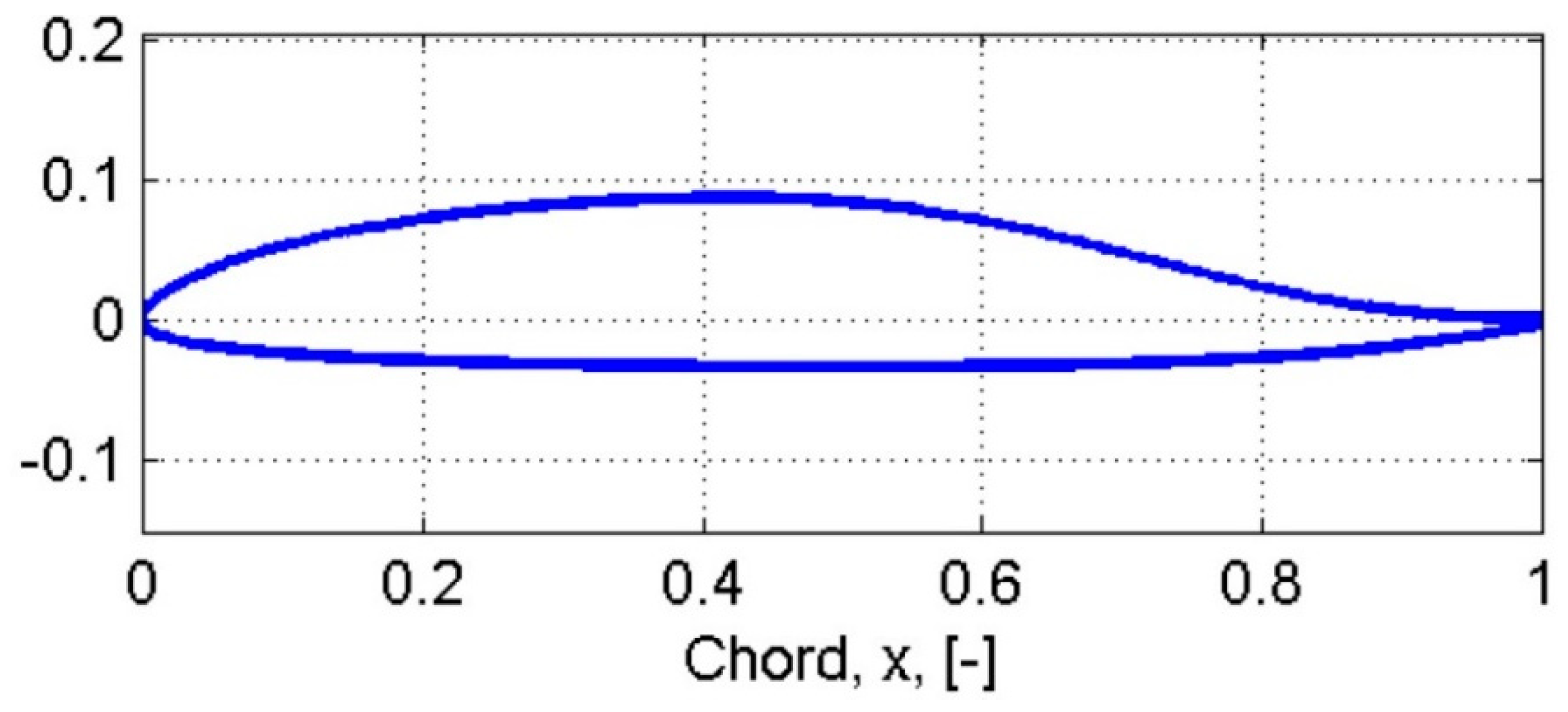
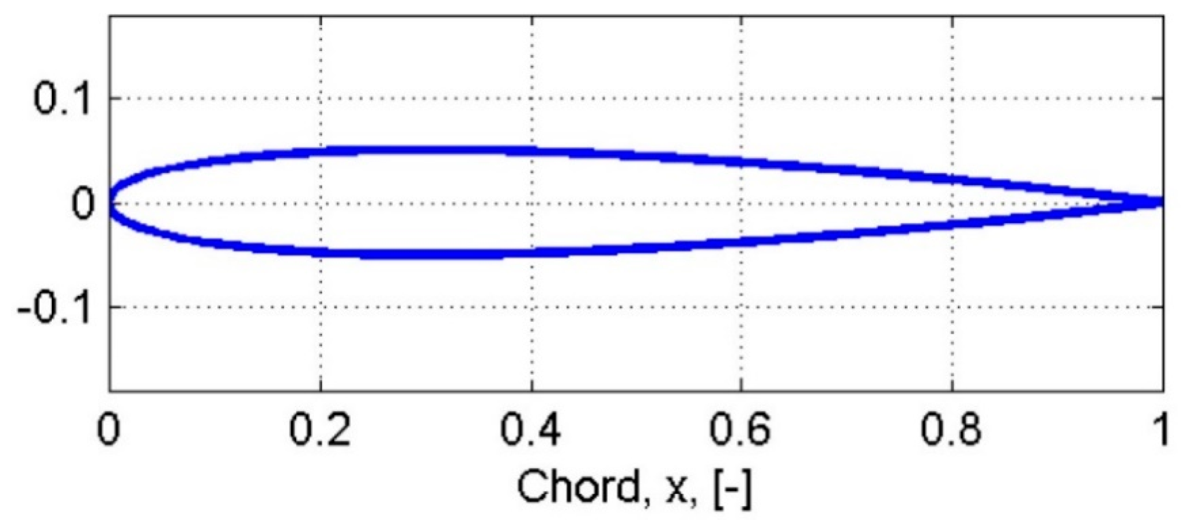
The car is designed using two airfoils (Roncz and NACA 10 [
22]), shown in
Figure 1 and
Figure 2.
Table 1 and
Table 2 show the geometrical properties of Roncz and NACA10, respectively. Roncz is used to design the top section,
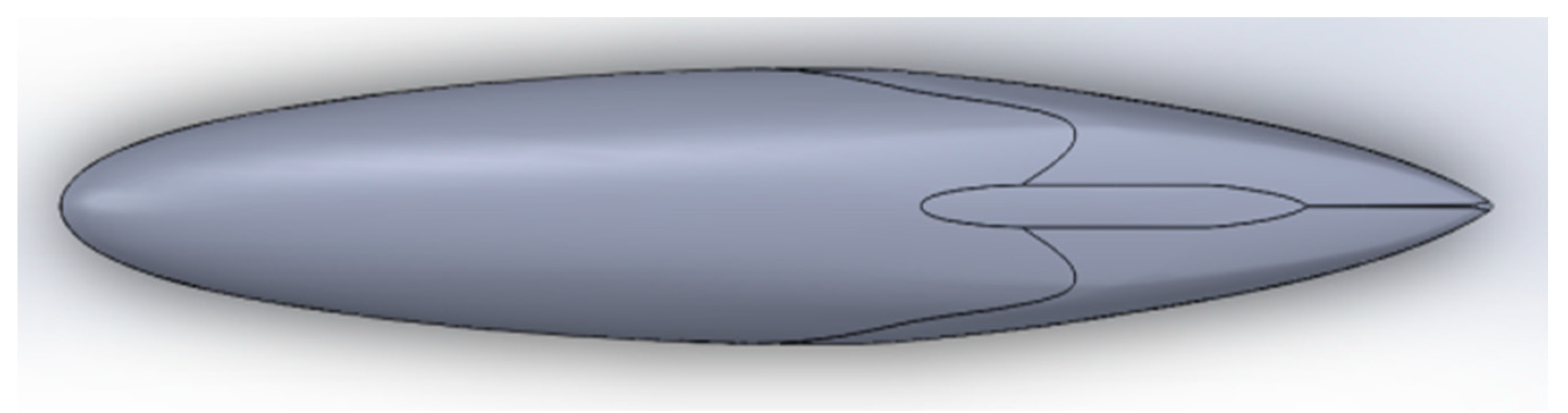
Figure 3. Only the front part of this airfoil is used to give the driver a comfortable and enough space to be able to drive the car. Moreover, NACA 10 Airfoil is used to design the side sections,
Figure 4. This combination of the two airfoils avoids any discontinuity; hopefully, it reduces the coefficient of drag.
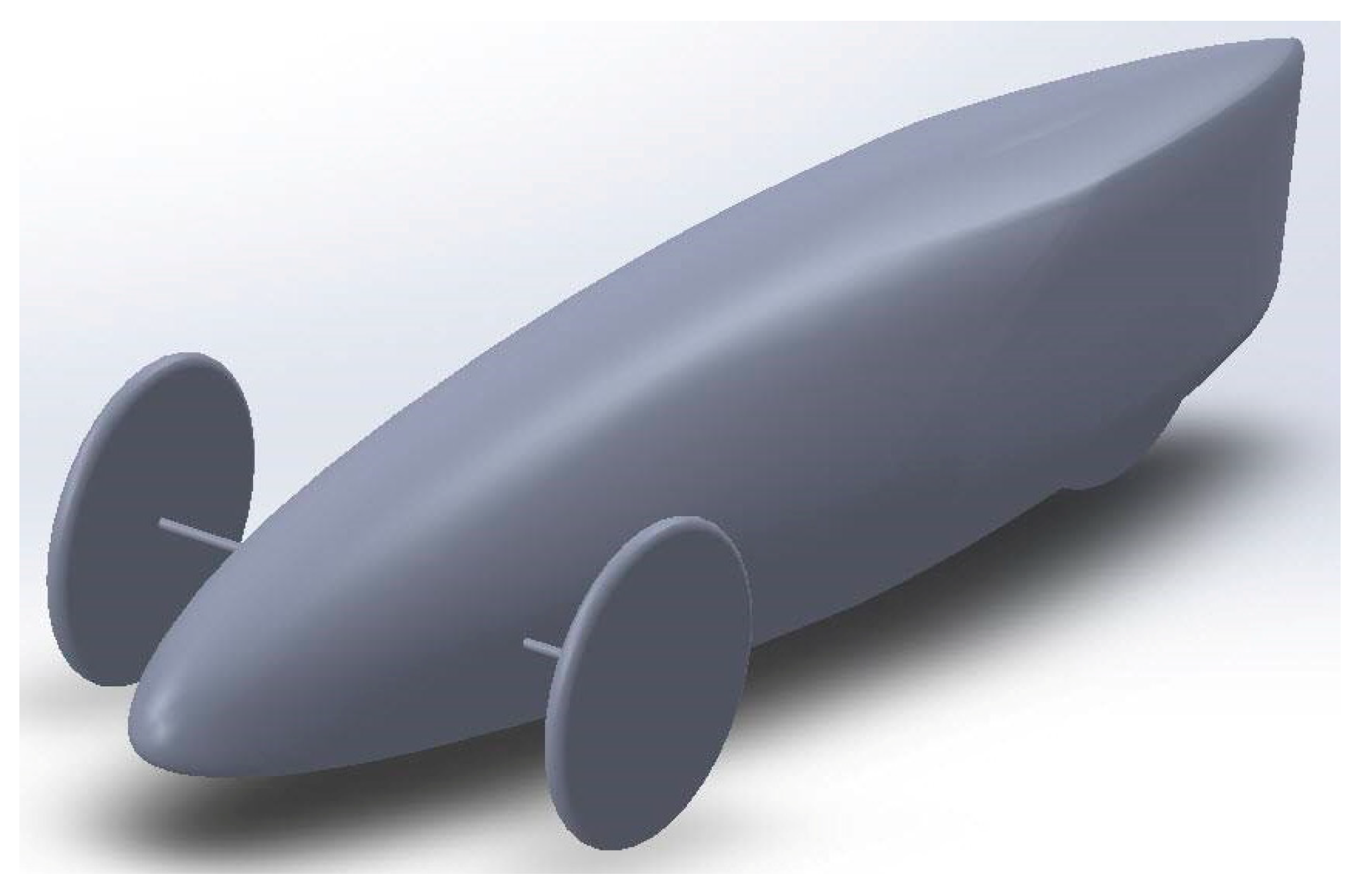
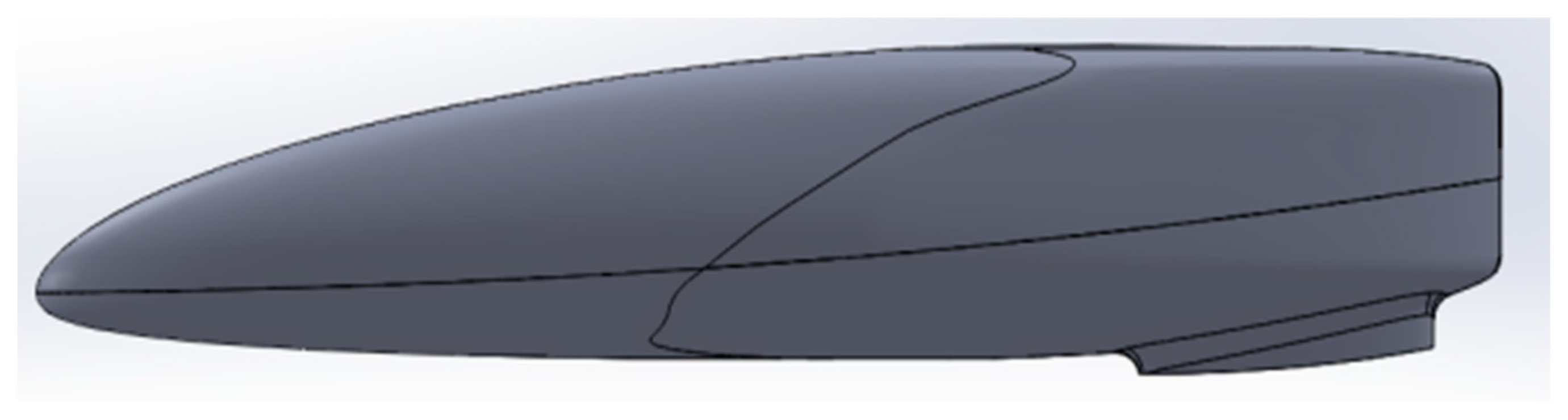
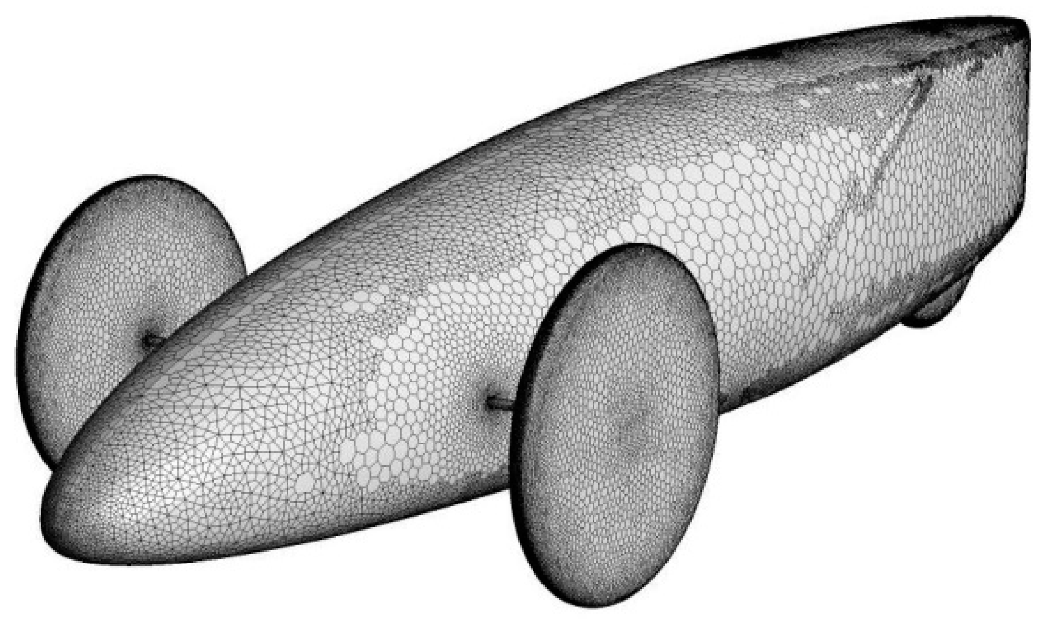
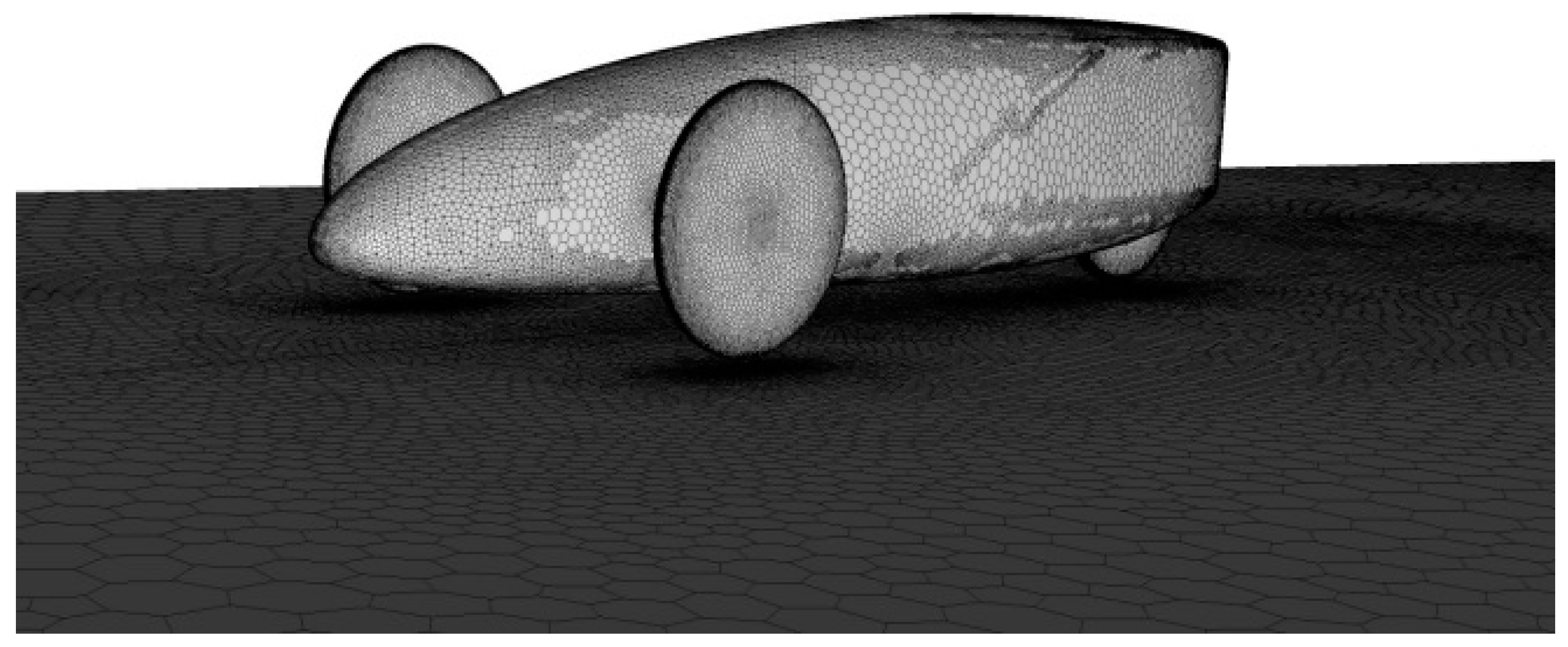
The car design, shown in
Figure 5, is a Computer Aided Design (CAD) drawing model. Its front tires are covered with fairing. This made the car body more streamlined. The car has only three tires (two at front and one at rear) to decrease friction losses.
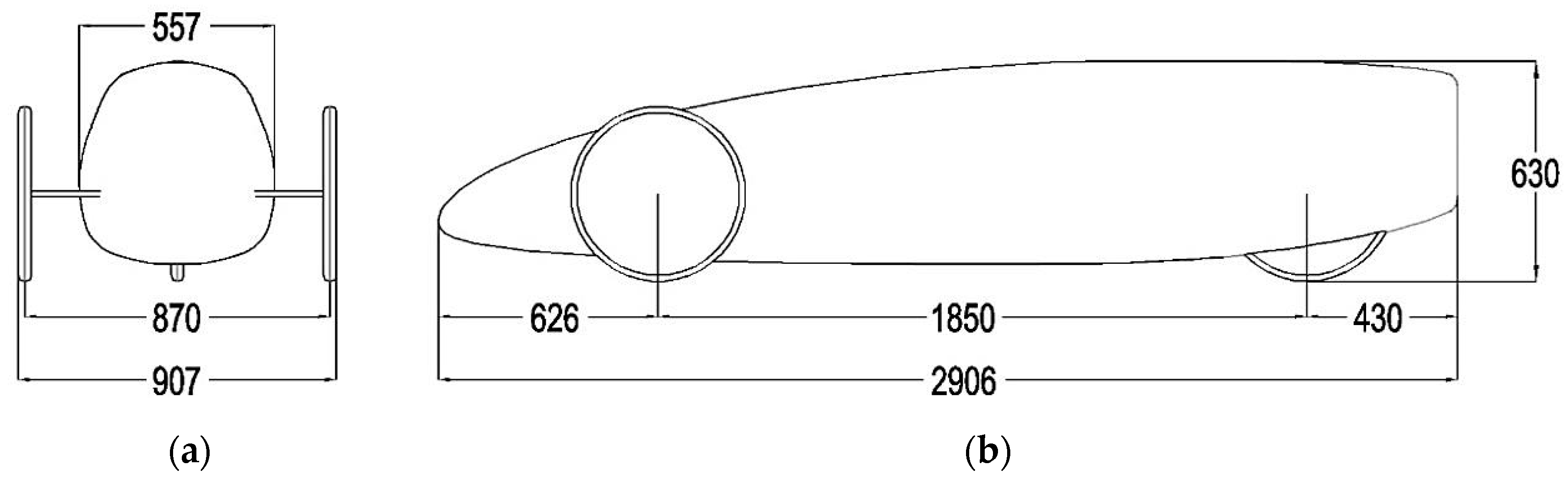
Figure 6 shows front and side views of the designed car. It has a maximum width, length and height of 907, 2906 and 630 mm, respectively. This car design has a frontal area = 0.2855 m
2.
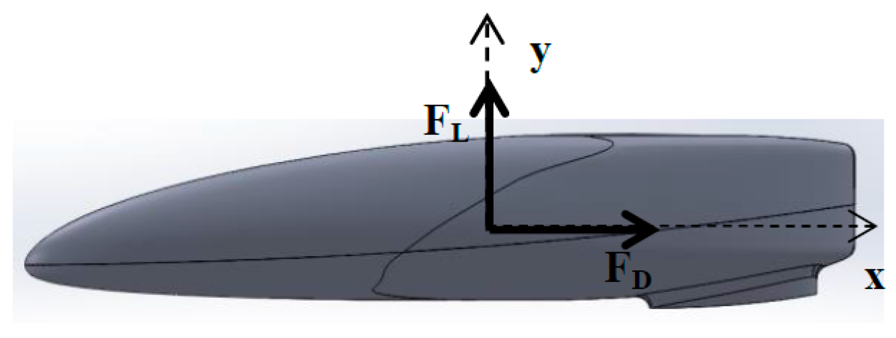
Drag force is one of the aerodynamic forces. It is the resistance force applied along the velocity vector,
Figure 7. Lift force performs perpendicular to the velocity vector, see
Figure 7.
The coefficients of drag (C
D), lift (C
L) and pressure (C
P) are given by the following equations:
Aerodynamic drag created on the car body affects fuel consumption [
23,
24,
25]. Modifications of car’s geometry can improve the flow around the car and reduce the aerodynamic drag. A relation between change in fuel consumption and change in drag coefficient is shown as follows [
26]:
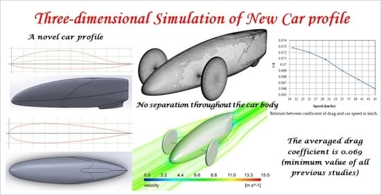
5. Results
Numerical simulation results provide parameters; coefficients of drag, lift and pressure and distributions of velocity and pressure, to declare whether the car profile is efficient or not.
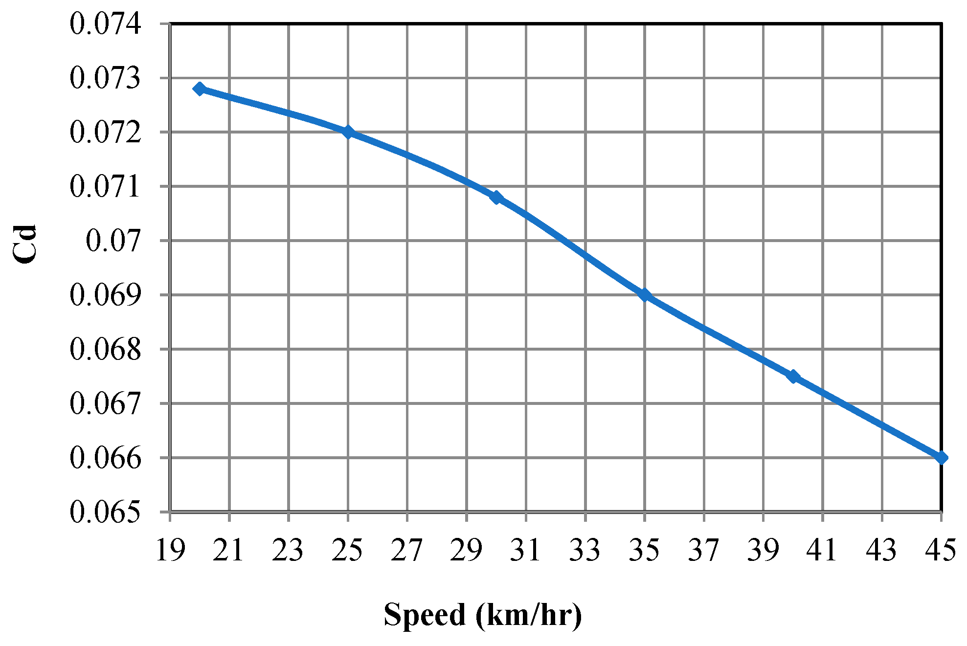
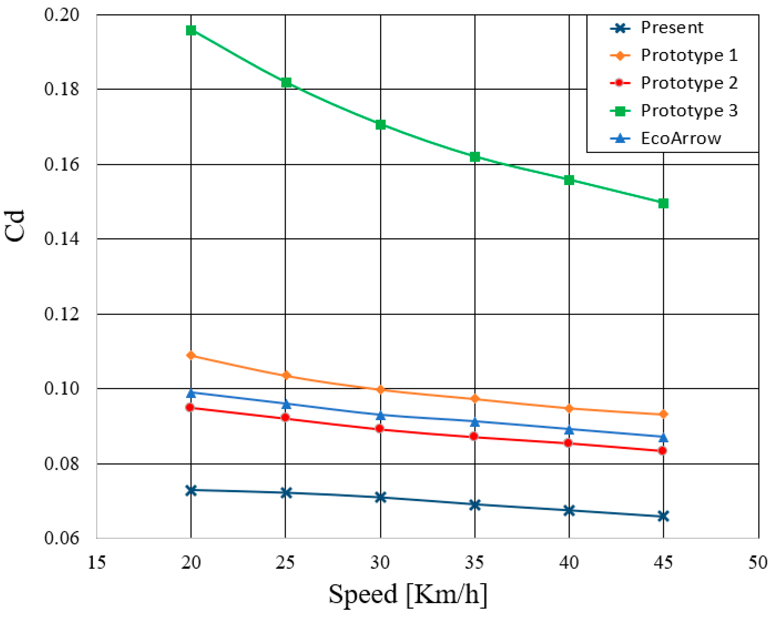
Drag coefficient is calculated based on integration of pressure and shear stress on the car surface. Relation between coefficient of drag and car speed in km/h is shown in
Figure 17. Coefficient of drag decreases slightly from 0.073 to 0.066 as the car speed increases over the range of velocity. The decrease in coefficient of drag is mostly due to low frontal length and the flow is always associated with the car body.
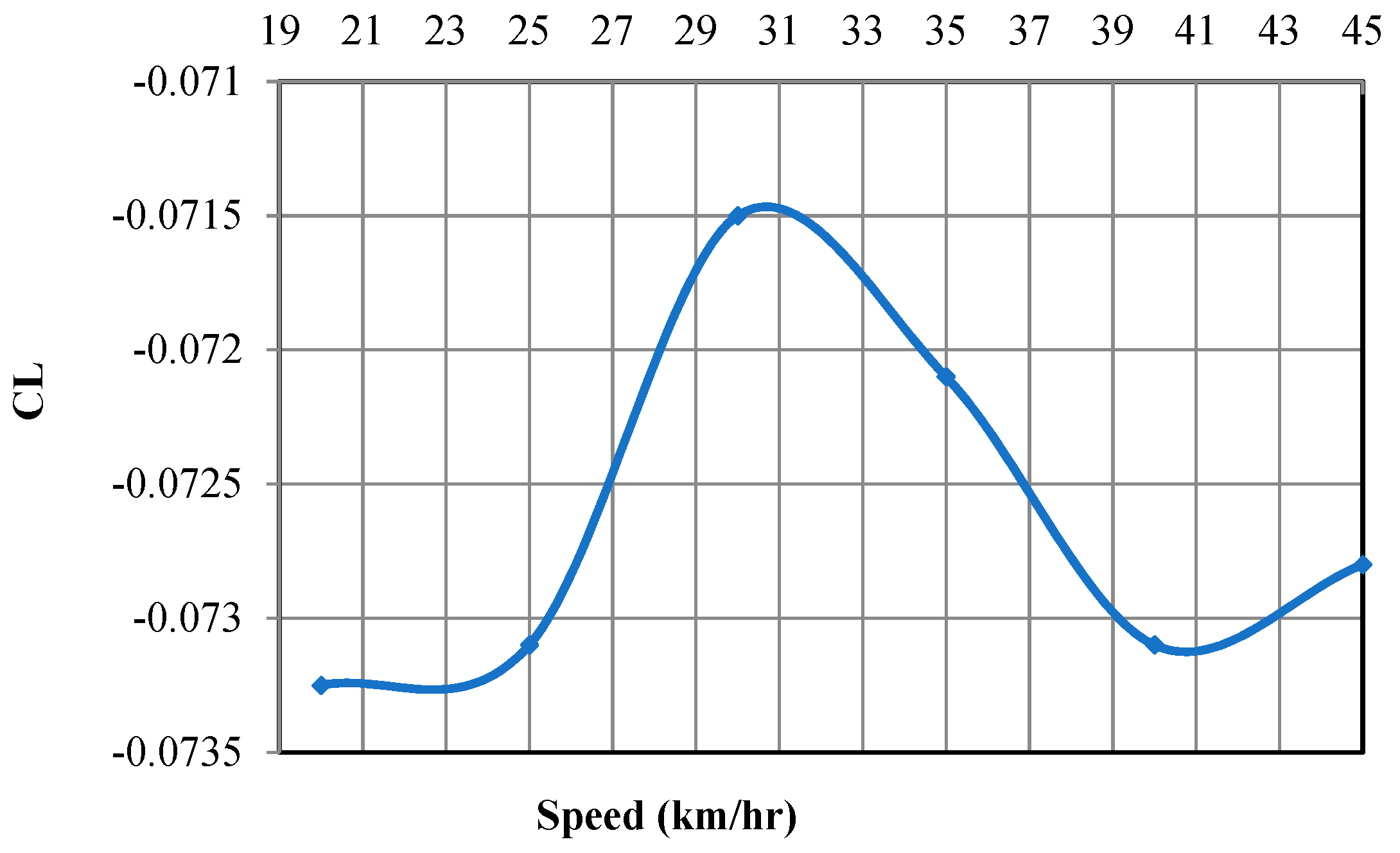
Relation between coefficient of lift and car speed in km/h is shown in
Figure 18. The coefficient of lift increases as the car speed increases from 20 to 30 km/h and then decreases from 30 to 40 km/h. C
L is a measure of the difference in pressure created above and below a car’s body as it moves through the surrounding viscous air. The slight change in the coefficient of lift value from −0.0733 to −0.0715 is due to small viscous effects of air.
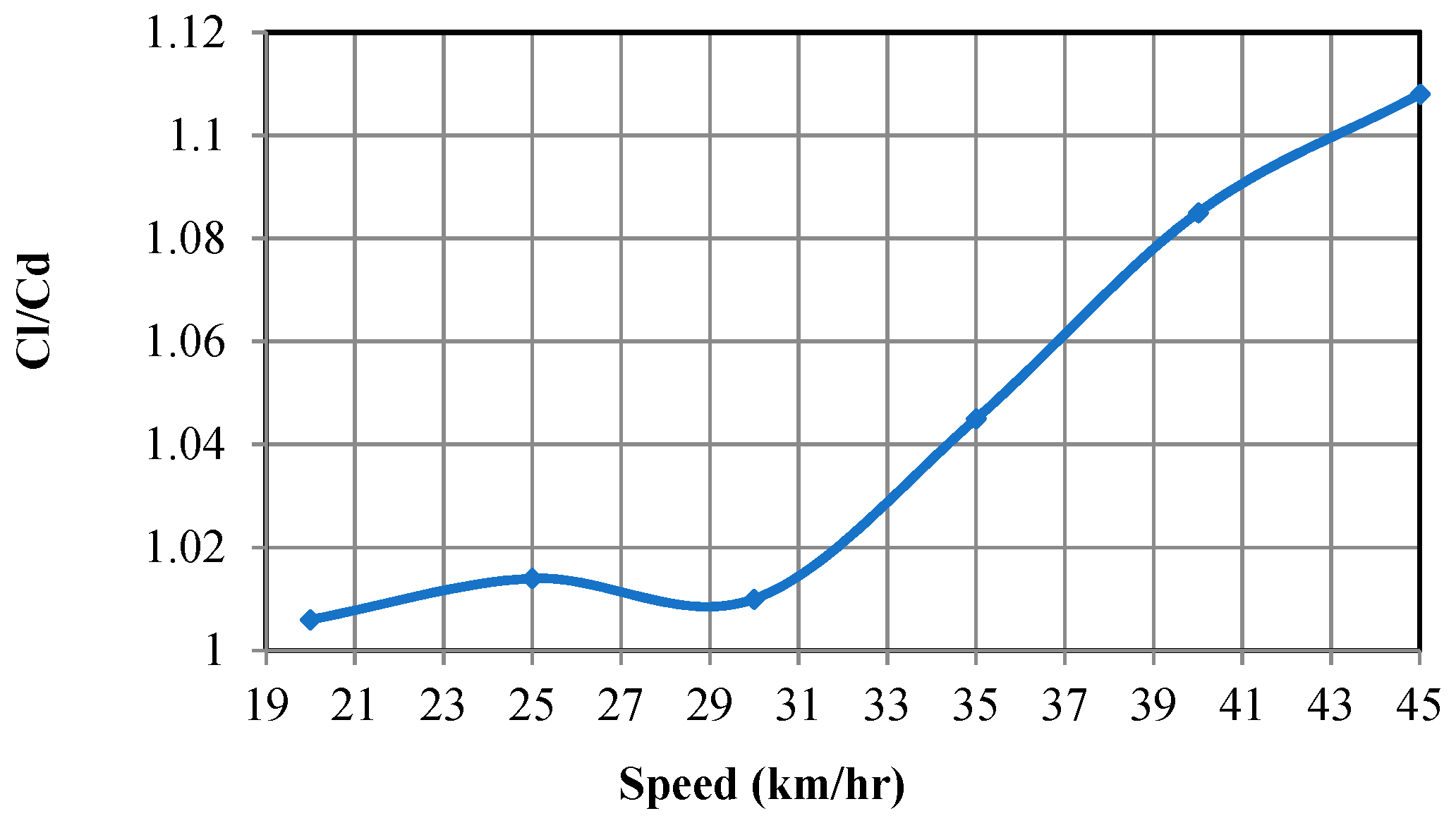
Lift to drag ratio, in aerodynamics, is the amount of lift produced by a vehicle divided by the drag created by movement through the air. As shown in
Figure 19, Cl/Cd is almost unified until the car reaches a speed of 30 km/h, after which the ratio increases linearly. This may be due to an almost constant coefficient of lift and increases the coefficient of drag.
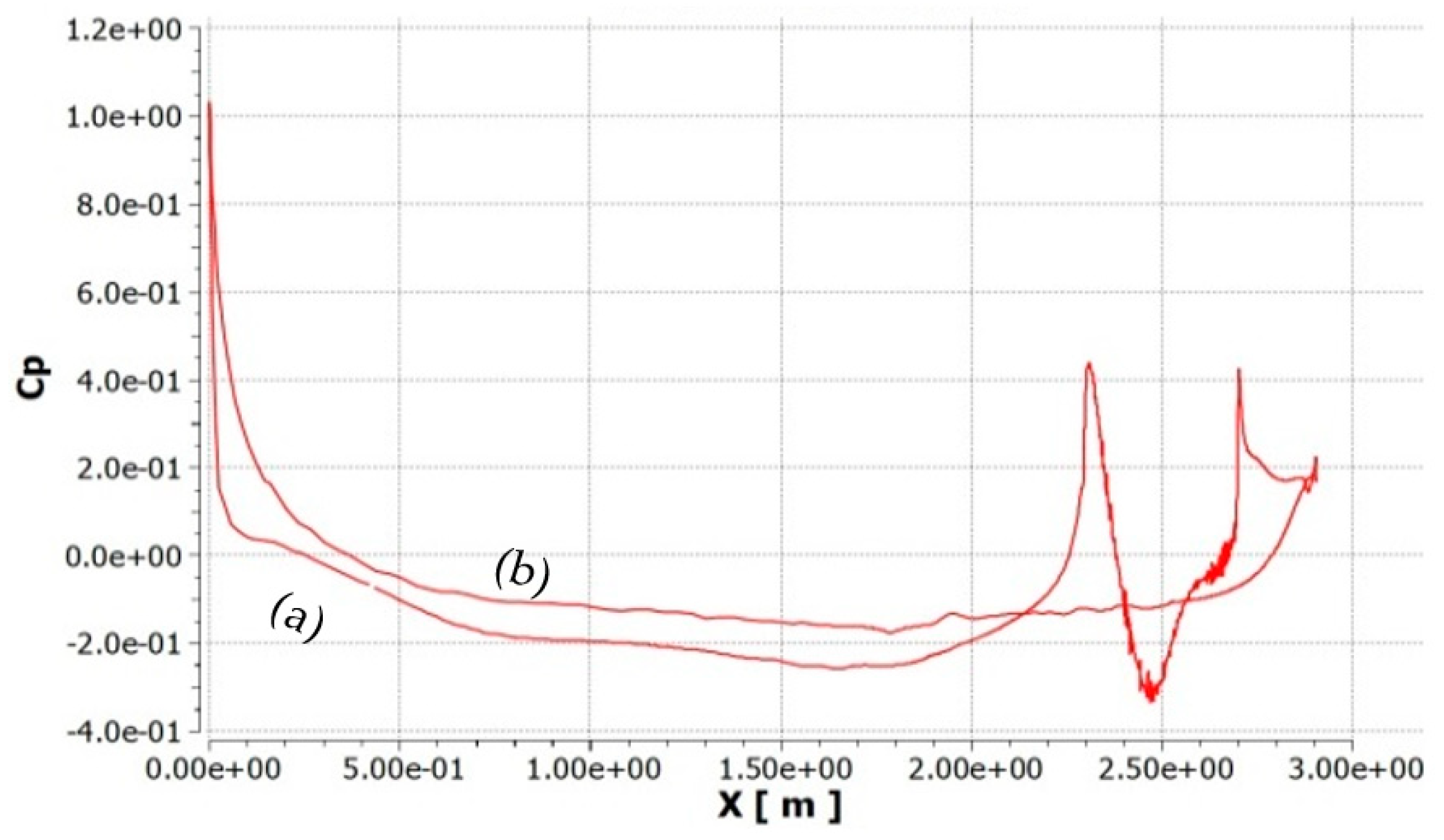
Figure 20 shows the pressure coefficient distribution at the middle vertical (x-y) plane of the car. The upper curve represents the bottom surface of the car and the lower curve represents the top one. Sudden changes in pressure are detected on the rear of the car. It can be observed that the positive pressure in front of the car is larger than that at the rear of the car due to some losses.
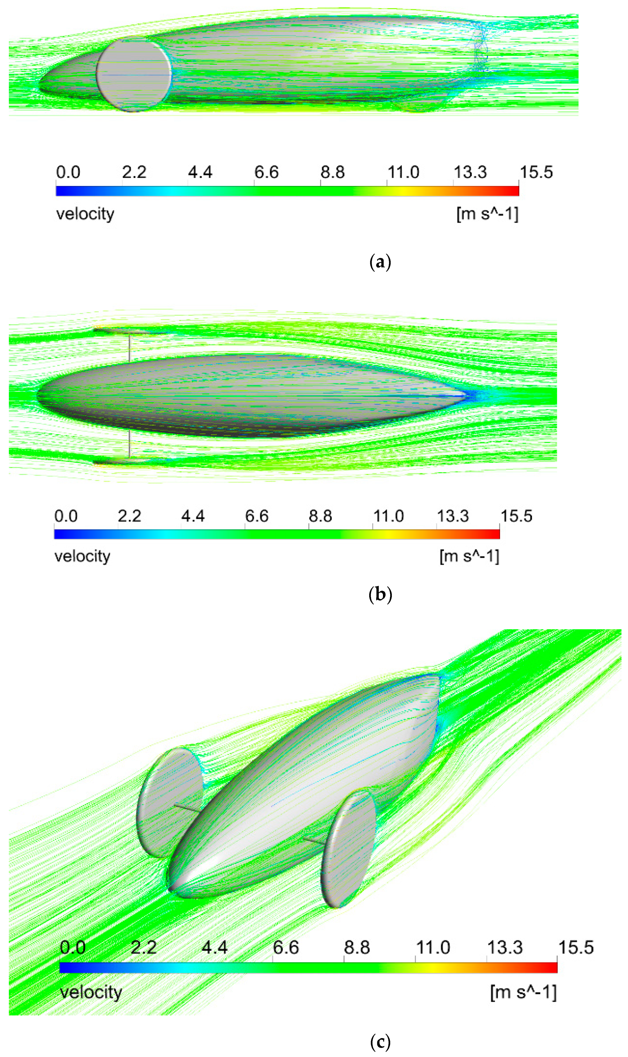
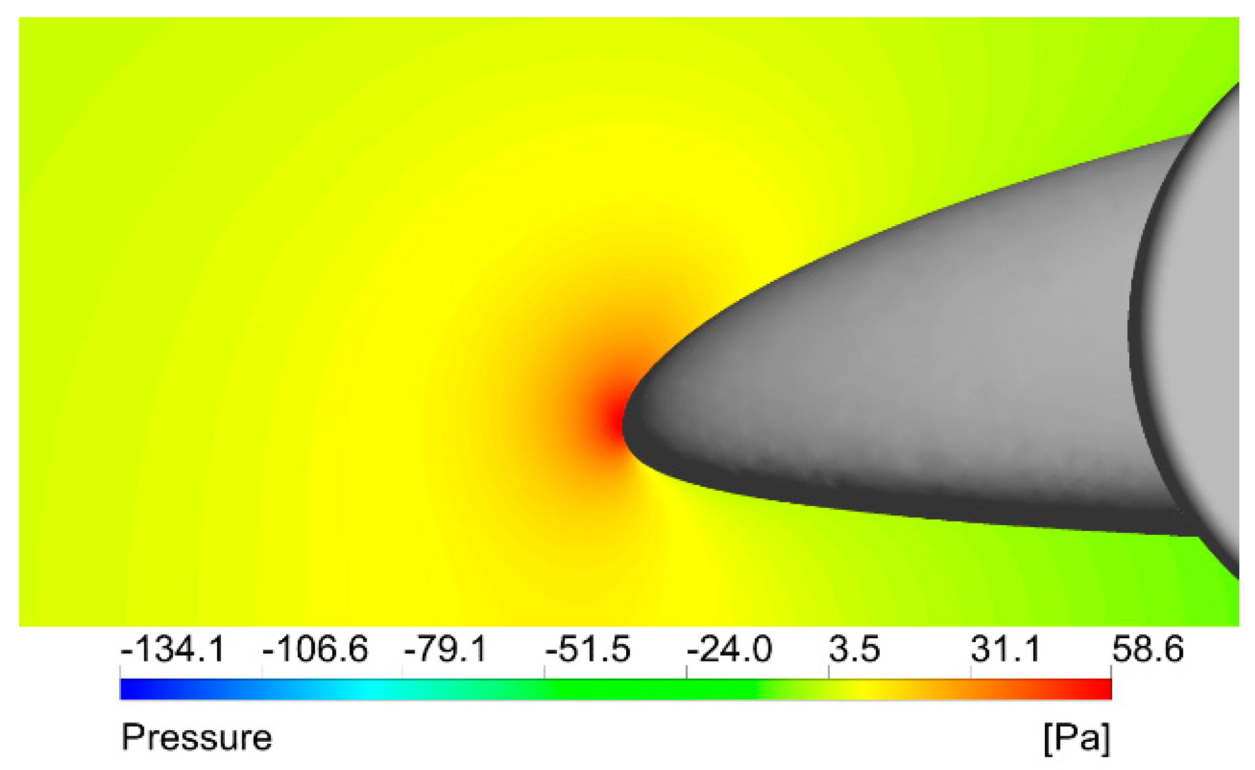
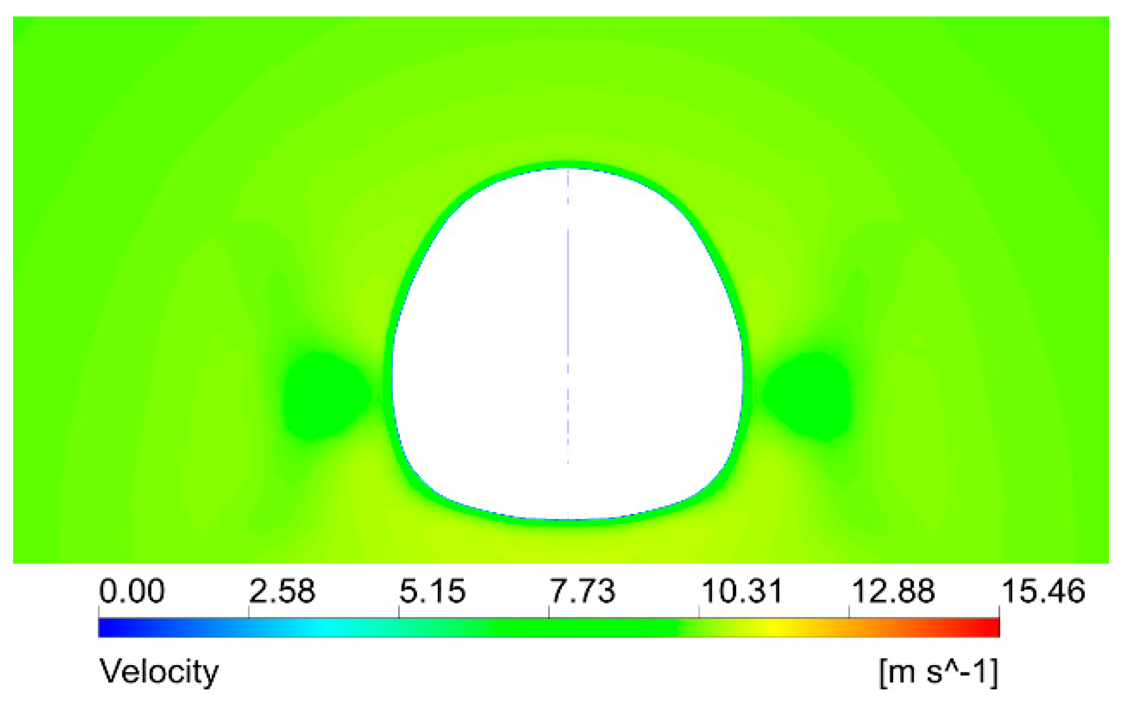
Air flow velocity and Pressure distributions on the car surface allow for the identification of the largest flow disturbances and the location of the highest pressure. Results of air velocity and pressure contours at a speed of 35 km/h (equals to 9.72 m/s) are shown in
Figure 21,
Figure 22,
Figure 23,
Figure 24 and
Figure 25.
Figure 21,
Figure 22 and
Figure 23 display air flow velocity distribution around the car. A quite clean pattern appears and smooth velocity distribution lines are successfully achieved. It shows a good aerodynamic performance. The color of the streamlines shows a typical expected increase in speed as it passes on the top of the car surface. The airflow pattern on the side of the car also shows no evidence of flow separation on a large scale. At the rear of the car, the airflow is smoothly attached to the car body and joins the main airflow stream, eliminating the flow separation zone. The flow shows no separation throughout the car body.
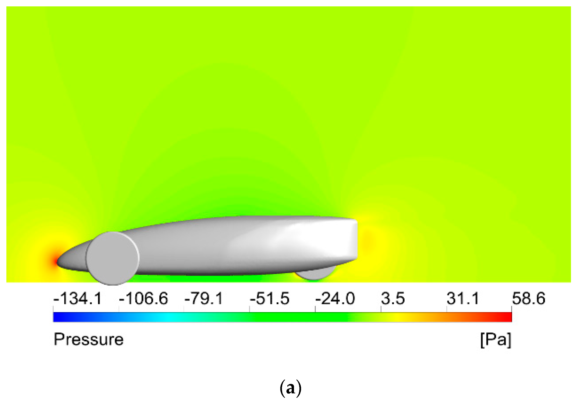
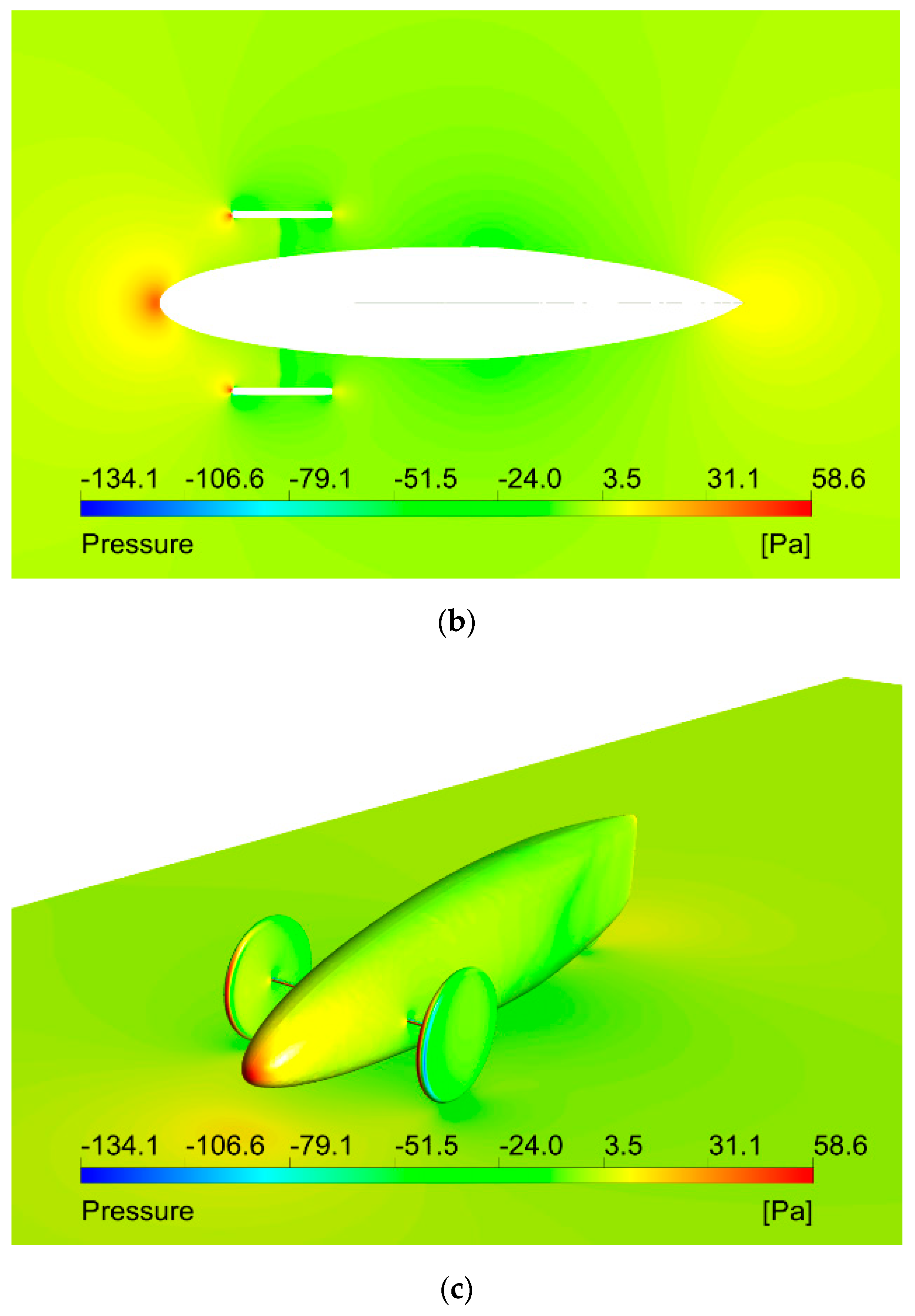
Figure 24 shows the static pressure distribution on the car surface. The maximum value of pressure appears at the front of the car because the fluid velocity on this area is close to zero. It reaches a value of 58.6 Pa, as shown in
Figure 25.


