Abstract
The microchannel flow model postulates that stress-strain behavior in soft tissues is influenced by the time constants of fluid-filled vessels related to Poiseuille’s law. A consequence of this framework is that changes in fluid viscosity and changes in vessel diameter (through vasoconstriction) have a measurable effect on tissue stiffness. These influences are examined through the theory of the microchannel flow model. Then, the effects of viscosity and vasoconstriction are demonstrated in gelatin phantoms and in perfused tissues, respectively. We find good agreement between theory and experiments using both a simple model made from gelatin and from living, perfused, placental tissue in vitro.
1. Introduction
Tissue elasticity measurements can provide valuable information related to pathological changes in tissues. Therefore, elastography has been extensively applied to the diagnosis of normal and abnormal conditions of tissues such as breast, liver, prostate, thyroid and placenta [1,2]. For example, Athanasiou et al. [3], in a study on 48 women with benign or malignant breast lesions, showed that elasticity of malignant lesions was higher than benign cases. Nabavizadeh et al. [4] compared the complex elasticity parameters such as storage and loss moduli and also the loss tangent of malignant versus benign breast tumors and stated that these parameters could serve as potential biomarkers. Wang et al. [5] reported a significant correlation between liver stiffness and fibrosis scores in 320 patients. Bavu et al. [6] in a study on 113 patients with hepatitis C virus used supersonic shear imaging (SSI) and showed that the SSI elasticity assessments are useful for evaluating fibrosis stages of the livers. In a study to investigate the tissue elasticity measurements for characterizing the normal versus cancerous prostate, Hoyt et al. [7] reported that the stiffnesses of cancerous prostates were significantly higher than the normal cases and suggested that tissue elasticity could be used as a cancer detection biomarker. Edwards et al. [8] summarized several studies that investigated the use of placental elasticity measurements in clinical applications. Kılıç et al. [9] in a study on 50 pregnant women showed that the placenta stiffness in patients with preeclampsia is substantially higher than the control groups. Hollenbach et al. [10] have shown that ischemic placental disease affects the shear wave speed (SWS), which correlates with elasticity, and suggested that elasticity imaging offers potential for placental disease discrimination.
Estimating the elasticity of tissues using appropriate mathematical/physical models is a fundamental need for reliable elastography measurements, and there have been different studies focused on that topic [11,12,13,14,15,16,17,18,19,20]. The microchannel flow model (MCFM) was proposed by Parker [21] as a descriptive and predictive model for elasticity quantification in soft, vascularized tissues. Under the assumption of the MCFM framework, the stiffness and SWS of vascularized tissues are related to the vasculature network parameters, the vessels’ fluid flow under stress, as well as the tissue parenchymal characteristics. In the derivation of the MCFM, time constants are introduced by employing Poiseuille’s flow law for the fluid inside the vessels, which are dependent on the fluid viscosity and the vessel diameter. Some pathological conditions could cause a change in the fluid flow parameters inside the vessel network, which under the MCFM framework reflects changes in the values of the time constant parameter associated with the vasculature. For example, inflammation in the liver [22], or the preeclampsia condition (a medical disorder in pregnancy that is associated with high blood pressure and the fluid flow reduction) in placenta [23,24] could both cause vessel constriction.
In this paper, we present experimental validations of the MCFM theory in predicting a relationship between the changes in characteristic time constants of tissues and the corresponding changes in their stiffnesses using tests on gelatin-based phantoms and also in vitro perfused placenta. Specifically, the effects of change in fluid viscosity and also vessel diameter (through vasoconstriction) on the time constants and therefore, on tissue stiffness, are investigated. The results from gelatin phantom experiments with interior fluid channels are employed to show the viscosity effect, and the in vitro perfused placenta experimental results are used to discuss the role of vessel diameter on the stiffness.
2. Theory
2.1. Background
The MCFM [21,25] begins with the analysis of a simple scenario, shown in Figure 1, where an elastic homogeneous material contains a small fluid-filled channel open on only one side.
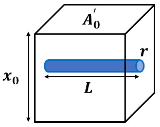
Figure 1.
An ideal model of an elastic, isotropic block with a single interior fluid-filled channel of radius and length is considered for the stress derivation in the MCFM. The block cross-sectional area and height are denoted by and , respectively. It is assumed that the channel is open to free exit of fluid volume only on one side, and the flow fluid is governed by Poiseuille’s law.
When placed in a stress relaxation test, we assume the resulting strain must account for both the elastic strain and the loss of volume as fluid is squeezed out of the channel under compression. A key assumption is that the fluid flow will be governed by Poiseuille’s law for laminar flow which states that the fluid flow undergoes a pressure drop of according to Equation (1), which is dependent on the fluid viscosity (), flow volume rate (Q), channel radius (r), and channel length (L). On the other hand, this pressure drop is physically proportional to the normal stress from the compression test sensed at the interior side of the microchannel (), with as a constant.
Assuming the decrease in volume of the fluid in the channel is reflected as the decrease in the volume (the length along the x-coordinate) of the tissue around it, the stress-strain relationship for the fluid-filled channel is derived in Equation (2) and simplified as Equation (3), which is analogous to a dashpot stress-strain relationship.
In these equations, is the strain applied, is the cross-sectional area of the tissue block, is the dimension along x, and C is a constant equal to . Considering the elastic medium and the fluid-filled channel as two elements undergoing relaxation results in a simple series spring-dashpot model with a single exponential decay given in Equation (4), the characteristic time constant associated with the fluid-filled channel is obtained from Equation (5).
In Equations (4) and (5), E is the Young’s modulus of the elastic medium, and is the magnitude of constant step strain applied. For the case of a vascularized tissue model, there will be a distribution of fluid channels with different radii corresponding to the distribution of vessels that result in having a spectrum of time constants, all contributing to the stress relaxation behavior. Using the superposition principle and integrating stress over a continuous distribution of relaxation time constants (channel sizes) assumed to follow a power law behavior , we have:
which is the two-parameter stress relaxation equation with b as the key power law parameter related to the fractal vasculature structure and as a constant, in which is the gamma function. Equation (6) is derived for a distribution of time constants from zero to infinity, however, in practice there are bounds on the largest and smallest vessels in a vasculature corresponding to larger veins and arteries and small capillaries and extracellular spaces, which map to the lowest and highest characteristic time constant, respectively. Applying these bounds on the integration over the relaxation time constant, the stress relaxation follows a four-parameter equation as shown in Equation (7) with two additional parameters of and where a = b – 1.
This framework makes specific predictions about the behaviors when either viscosity is changed, or vasodilation or vasoconstriction causes a change in vessel radii.
2.2. Change in the Relaxation Time Constant Associated with the Fluid Type
In theory, when viscosity is changed in the simple channel-in-phantom (CIP) model shown in Figure 1, we simply have a change in the stress relaxation time constant and the stress level. In the derivation of the MCFM, each channel contributes to the relaxation with a distinct characteristic time constant according to Equation (5). The time constant increases linearly with the increase in the viscosity of the fluid inside the CIP and decreases with the stiffness level of the phantom; the more viscous fluid and also the softer background case have higher time constants. Therefore, a change in the fluid viscosity would have the effect of changing the stress relaxation response in experiments, assuming all other parameters remain constant.
2.3. Change in the Relaxation Time Constant Associated with Vessel Size
By definition, any vasoconstriction or vasodilation in vascularized tissues such as placenta imposes a change in the vessel radii. Introducing a scale factor , the relationship between the radii of the changed states after vasoconstriction/vasodilation and the initial state is modeled as:
The state of the vasculature after vasoconstriction/vasodilation have a new relaxation spectrum as well as new maximum and minimum time constants denoted by and , respectively. The parameters of the second states of vasculature are related to that of the initial states by employing the general transformation rule explained in detail in Parker [26], which are shown in Equation (9) (which is true for and as well) and Equation (10).
The stress relaxation response for the new vasculature is obtained by integrating over the new relaxation spectrum, shown in Equation (11).
The vessel radii scale factor is found as the key parameter in linking the two states of the vasculature before and after undergoing the vasoconstriction/vasodilation. Vasoconstriction, characterized as the case with , causes an increase in time constants as well as a general hardening of the tissue in comparison to the baseline state.
Therefore, vasoconstriction/vasodilation experiments in living tissues undergoing changes in the vessel radii are another way to study the effect of changes in the characteristic time constants on the tissue response.
2.4. Ramp-Plus-Hold Models for CIP
The stress relaxation behavior of a material is characterized by its response to the application of an ideal step strain function on the sample of the material. However, an ideal step strain involves imposing an instantaneous change of strain from zero to the desired strain which, in practice, cannot be achieved physically. Therefore, a step strain is modeled as a combination of two processes: first, a gradual linear increase of strain from zero to a desired strain level in the form of a ramp with the duration of , and second, keeping the strain constant, allowing the viscoelastic material to relax in time, as show in Figure 2a, similar to the derivation of stress response using the Kelvin-Voigt fractional derivative (KVFD) model by Zhang et al. [27].
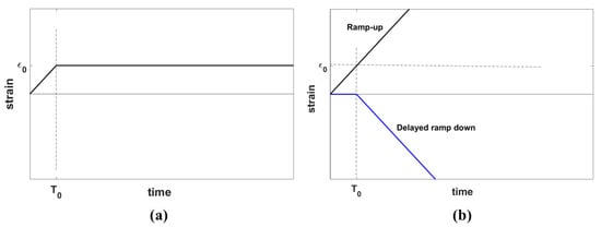
Figure 2.
(a) A ramp-plus-hold strain function representing the experimental step strain applied in practice for the stress relaxation test and (b) an equivalent representation of the strain function in (a) composed of a ramp-up strain function plus a delayed ramp-down strain function. The parameter indicates the hold strain and shows the ramp duration.
Applying ramp-plus-hold strain is equivalent to the superposition of a ramp-up strain and a delayed ramp-down strain, as depicted in Figure 2b. The same rule applies to the stress response according to Equation (3):
From systems theory, the response of a linear system to the ramp input is the integral of the response to the ideal step input. Thus, for the CIP with fluid, the ideal step response in Equation (13) is employed to derive Equation (14) as the CIP ramp response. Equation (13) expresses the stress contribution from a CIP filled with fluid in response to the ideal step strain with the time constant of introduced by the CIP, and is a constant.
By substituting Equation (14) into Equation (12), the CIP ramp-plus-hold response can be easily obtained. To focus mainly on the role of the fluid inside the vessels in the characteristic time constant, we consider two experiments where the elastic block is the same for both cases, but the viscous fluid in the CIP is different. If subscripts (1) and (2) correspond to the cases with fluid (1) and fluid (2), respectively, then the stress difference between these two cases when subjected to ramp-plus-hold strain is given by:
where denotes the difference between the total stresses for the two cases.
3. Methods
3.1. Phantom Preparation
For making the CIP samples, four small plastic rectangular cubes were made as the molds with a cross section of 35 mm × 35 mm and a height of approximately 38 mm. Each mold had 6 circular slots with diameters of 3 mm for inserting disposable plastic straws to make the CIPs. The arrangement of the CIPs (or straws) are shown in Figure 3a,b. The channels are placed inside the cubes at a slight angle of approximately 5° as shown in Figure 3c to avoid the fluid flow out of the CIPs during the experiment.
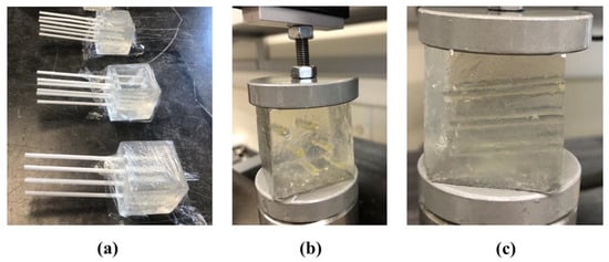
Figure 3.
(a) Samples of gelatin-based phantoms each including six channel-in-phantoms (CIPs) made by sealed straws which are removed when the gelatin mixture hardens to produce channels. (b) and (c) show the front and side views of one of the samples from (a), respectively undergoing the stress relaxation test after injecting castor oil inside the CIPs.
Gelatin-based phantoms are made from a specific mixture of gelatin, agar, sodium chloride (NACL) in 900 mL of degassed water with the weight proportions of the ingredients listed in Table 1 [28].

Table 1.
Portion of ingredients used for making phantoms.
The phantom preparation procedure was similar to the method used in [28] and is described here. For making a homogeneous gelatin phantom, the gelatin powder, agar, and NaCl were mixed and the mixture was added slowly to the degassed water while stirring to let the ingredient dissolve. Then, the mixture was heated up to a temperature of about 65 °C and then was placed on a magnetic stirrer to stir it constantly. By placing an ice bath around the container, the solution was allowed to cool down to nearly 30 °C. The straws were sealed using wax and then inserted in the cubic mold before adding the gelatin mixture into the molds. The samples were left at a temperature of 4 °C overnight to let the gelatin mixture solidify. On the next day, the phantoms were allowed to reach room temperature before performing the mechanical testing.
3.2. Stress Relaxation Test
The compression test for stress relaxation measurements was done by applying a 5% strain on each sample using a Q-Test/5 machine (MTS, Eden Prairie, MN, USA) with a 5 N load cell and a compression rate of 0.15 mm/s for approximately 500 s of relaxation time. The ramp-plus-hold time was approximately 12–13 s depending on the sample height. The test was done on 3–4 samples of gelatin phantoms with castor oil and also with olive oil as the CIP fluid. The relaxation force measured during the test was converted to stress using the cross-sectional area of the samples. Then, the difference in the stress variation in time of the castor oil CIP samples and the olive oil CIP samples was fitted to a stress vs. time relationship similar to Equation (15) to obtain the coefficients. A slightly modified version of Equation (15) was used in the curve-fitting procedure with an additive constant included. This additional constant allows for some flexibility in the fitting process and accounts for small experimental sample-to-sample differences.
Stress curve fittings were performed using the curve-fitting toolbox in MATLAB (MathWorks, Inc., Natick, MA, USA) based on the nonlinear least square minimization of errors.
3.3. Viscosity Measurement
Noting that the viscosity of the fluid plays a major role in the value of the time constant, the viscosities of the two fluids employed are measured at lab temperature using a viscometer (Cannon, model 9721-B74, universal size 400, State College, PA, USA). Using the time period required when a fluid inside the viscometer flows between two marked points and also the characteristic viscometer constant provided by the manufacturer, the kinematic viscosity of the two fluids are calculated and then converted to the dynamic viscosity for each fluid using the density of the fluids. The characteristic viscometer constant is 0.4511 cSt/s at room temperature.
3.4. Placental Elastography Images and SWS Measurements
Elastography images of the in vitro perfused human placenta were obtained at a center frequency of 5 MHz using a Siemens Antares scanner (Siemens Medical Solutions, Malvern, PA, USA) and a VF10-5 probe (Siemens Medical Solutions, Malvern, PA, USA) with a single-track location shear wave elasticity imaging (STL-SWEI) pulse sequence and accelerated processing [29]. To study the shear wave propagation in the placenta, the velocity versus time data were obtained at two locations after applying a radiation push pulse and then, by employing the Fourier transform, the amplitude and phase of the velocity were obtained as a function of frequency.
Placenta tissue under this study was from a healthy pregnancy immediately after caesarean section with no overall defects observed during post-delivery examination. Using an open perfusion system, an arterial pressure of <40 mmHg and a normal fetal flow at about 3–6 mL/min were maintained. For creating in vitro vasoconstriction in the perfused placenta, a dose of 1 mL 10−6 M vasoconstrictor agent (thromboxane agonist, U46619, Caymen Chemical Co., Ann Arbor, MI, USA) was injected in the fetal artery.
The protocol for this study was approved by the Research Subjects Review Board at the University of Rochester. The placenta is a disposable tissue specimen from the surgical examinations and no patient is identified related to the disposable samples. Therefore, consent from the patient was not needed, consistent with the World Medical Association Declaration of Helsinki.
4. Results
The results are presented in two sections: first, the results from the stress relaxation tests on the CIP gelatin phantoms with fluid channels are presented. The second section includes elastography results on the perfused placenta in baseline and vasoconstriction conditions.
4.1. Phantom Experiments
4.1.1. Viscosity Measurements
The viscosities of castor oil and olive oil are measured using the viscometer and the average of measurements and the standard deviation for each case are reported in Table 2. The measurement for each oil is repeated 4–5 times and the low standard deviation for both cases indicates the reproducibility of the measurements. The results show that castor oil is almost 12 times more viscous than olive oil.
Table 2.
Mean viscosity measurements of the selected oils and their standard deviations (SD) at room temperature.
4.1.2. Stress Relaxation
Figure 4a,b show the results of stress relaxation tests on gelatin-based phantoms with castor oil and olive oil channels, respectively. The stress curves of different samples of the same fluid inside CIP being similar indicates the good reproducibility of the test. Also, comparing the stress level for the two groups, it is observed that the samples with castor oil have elevated stress in comparison to the samples with olive oil, and appear stiffer in the experiment.
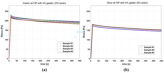
Figure 4.
Stress relaxation curves for phantoms having: (a) channels filled with castor oil (b) channels filled with olive oil, all resulting from 5% strain. For castor oil, the test results of four samples and for olive oil the test results for three samples are presented.
Figure 5a–d show four examples of the MCFM curve fits to the stress differences of samples with castor oil CIPs and samples with olive oil CIPs, and Figure 5e presents the fitting results when the averages of all stress differences of the two groups are taken into account. The results of fitting parameters are reported in Table 3 with the value of fitting goodness evaluated by R2. The fitting results for the two time constants show that the higher time constant (which is associated with the castor oil) is, on average, approximately 12 times larger than the smaller time constant (which is associated with the olive oil).
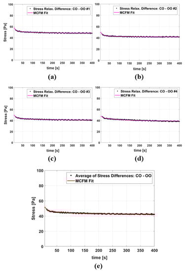
Figure 5.
(a–d) The MCFM fit to the stress relaxation differences between some individual castor oil CIP samples and olive oil CIP samples, all tests done under 5% strain. (e) The MCFM fit to the average of stress relaxation differences.
Table 3.
MCFM fitting results.
4.2. Perfused Placenta In Vitro Elastography
Figure 6a shows the elasticity measurements as a color image overlaid on the B-scan of the perfused placenta and Figure 6b illustrates the shear wave generated in the tissue due to the application of acoustic radiation force push pulses at two locations that are used for elastography measurements.
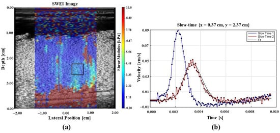
Figure 6.
Elastography results from an in vitro perfused placenta. (a) B-scan image with tissue stiffness as a pseudo-color overlay with the color bar showing local stiffness in the region of interest. Blue color represents softer and red indicates stiffer regions. (b) Shear waves from radiation force push pulses at 2 locations. These data form the basis of elastography measurements.
Figure 7 presents the SWS dispersion curves for baseline and the vasoconstriction condition for the perfused post-delivery placenta. Introducing vasoconstrictor agents causes a decrease in vessel diameters and, therefore, an increase in the SWS measurements. The higher level of SWS for the vasoconstriction implies that the tissue is stiffened in comparison to the baseline. In this figure, the SWS dispersion measurements are presented as four datasets for baseline, and three datasets for vasoconstriction, shown as different yellow symbols and green symbols, respectively.
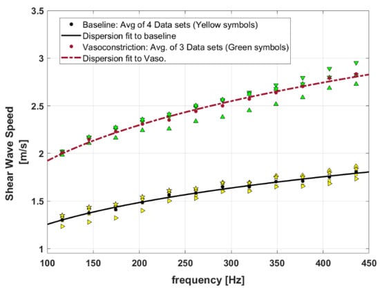
Figure 7.
Shear wave speed dispersion curves for the baseline perfused placenta versus placenta in vasoconstriction. Yellow symbols show four different datasets from baseline measurements and green symbols present three different datasets from vasoconstriction measurements. The fitted curves are results of power-law fitting to the average of measured datasets for each condition (baseline and vasoconstriction).
The MCFM framework predicts a power law frequency-dependent elasticity and SWS for the soft vascularized tissues as and with as the power law parameter related to the vasculature networks of the tissues () and [30]. Therefore, the curve fit to the dispersion of SWS for baseline and vasoconstriction can approximate the key power law behavior at the two states. In Figure 7, the power law curve fits to the averaged SWS dispersion measurements for each condition are shown as lines, and the fitting coefficients are reported in Table 4. The results indicate that the power-law parameter (or b) from the SWS dispersion measurement fitting is slightly higher in vasoconstriction in comparison to the baseline.
Table 4.
Power law fitting to dispersion of SWS: .
5. Discussion
Employing the MCFM offers the potential to investigate the role of the fractal vasculature of tissues and the fluid contents as they influence tissue stiffness at a macroscopic scale. According to the MCFM derivation, each vessel in a vasculature is associated with a characteristic time constant and therefore a branching vasculature, comprised of different vessels from smallest to largest, introduces a spectrum of time constants that contribute to the behavior of the soft tissue under study. Under the MCFM, an increase in the time constant elevates the stress relaxation level and the stiffness of the tissue. The time constant of the MCFM depends on a number of parameters such as the viscosity of fluid inside vessels, the vessel radius and the elastic modulus of the tissue around the vessels according to . It appears that there are some pathological changes in tissues that could change these parameters and therefore, could change the distribution of time constants within these tissues. For example, the placenta is a vascularized organ that is vital for development and survival of the fetus and acts as a connecting medium between mother and the fetus. In some complicated cases like pregnancy-induced hypertension, placental blood flow could decrease, imposing some risks to the fetus [31]. These pathological changes in the placenta may relate to changes in the characteristic time constants in the MCFM. Therefore, the MCFM framework has the potential to characterize and model some pathological changes of the tissues. This work has presented some experimental validations for the effect of time constant variation on the stress and stiffness level of phantom/tissue predicted by the MCFM through separate tests on the gelatin-based phantoms and also in vitro perfused placenta. It is shown that the MCFM predictions of the effect of time constant on the stress/stiffness level are consistent with the experimental observations in the two experiments.
In gelatin-based phantom experiments, it is shown that when fluid within the CIP is changed from a low viscous oil (olive oil) to a fluid with higher viscosity (castor oil), the stress relaxation curves shift to higher values under the same strain applied in the test. Moreover, it is shown that the MCFM fits well to the stress differences of olive oil CIP samples and castor oil CIP samples, containing two fitted time constants where the larger one (which is associated with the castor oil) is approximately 12 times larger than the smaller time constant (which is associated with the olive oil) in the fitting process. This is close to the range predicted by the theory using the associated parameters as:
where, by substituting our experimental parameters into Equation (5):
which is approximately close to the time constant estimated for castor oil from the stress relaxation curve-fitting reported in Table 3, and indicates the agreement of the MCFM prediction in theory and the experiment.
Next, considering the fractal vasculature within the placenta, the injection of the vasoconstriction agent imposes a decrease in the radii of vessels, which also results in an increase in arterial pressure. The elevated dispersion curve for the vasoconstriction condition in the placenta demonstrates that vasoconstriction imposes a stiffening effect on the tissue. In these experiments, the arterial pressure under a constant flow pump increased from approximately 40 mmHg to 90 mmHg after vasoconstriction. Under Poiseuille’s law, this corresponds to a decrease in radius to the fourth power using Equation (1), which is related to the vessel radii scale factor according to Equation (8). The relationship of the arterial pressure change with the vessel radii scale factor can therefore be written as:
We can roughly estimate how the stress behavior and therefore, the stiffness level of the placenta could change between baseline and the vasoconstriction state with the scale factor of . Borrowing from the dispersion fitting results presented in Table 4, the power law parameter ) approaches 1.5 for the vasoconstriction. Using Equation (11) for the stress response when is equal to 1.5, the leading term in simplifies, predicting a new stress response changed approximately by . This implies that the stress level increases and the tissue becomes stiffer due to vasoconstriction . In our case, the prediction from theory is that the post-vasoconstriction stress relaxation would be elevated by a factor of (1/0.817)2 which is approximately 1.5, very close to the proportional change shown in Figure 7.
Specifically, by examining Figure 7 and the fitting results in Table 4, the second fitted parameter c’ from the SWS dispersion fitting for the baseline and vasoconstriction is 0.412 and 0.589, respectively. The proportion of these two parameters is 0.589/0.412 = 1.4 which indicates a higher level of c’ for vasoconstriction, consistent with the earlier estimate following Equations (18) and (19).
Thus, the leading term defined in the MCFM derivations in Equations (7)–(11) appears to adequately predict observed changes in tissue stiffness caused by vasoconstriction.
6. Conclusions
By employing Poiseuille’s law of fluid flow, the MCFM introduces a characteristic time constant associated with each vessel in a vasculature that is found to affect the stress-strain behavior in the underlying vascularized soft tissue. In this study, by using two separate experiments in gelatin-based phantoms and also perfused post-delivery placenta, the effect of changing this time constant on the tissue behavior is investigated. Under this framework, we examined the changes in two separate parameters:
- vessel fluid viscosity (in phantom experiments)
- vessel diameter (through vasoconstriction in placenta).
The associated time constants were changed, and it is shown in both cases that increasing the characteristic time constants creates a stiffening effect on the tissue/phantom under study through increased stress relaxation level in phantoms and elevated SWS dispersion in placenta. The degree of change is also consistent with the prediction of MCFM. Thus, the MCFM can be useful for stress-strain models of vascularized tissues including changes over time as pathologies or vasoactive responses are activated.
Author Contributions
Conceptualization, K.J.P.; methodology, S.S.P.; software, S.S.P. and J.O.; investigation, S.S.P., J.O. and S.J.H. All authors have read and agreed to the published version of the manuscript.
Funding
This research was supported by the National Institutes of Health, grant number R21EB025290.
Acknowledgments
We are grateful for experimental help from Richard K. Miller and Ronald W. Wood.
Conflicts of Interest
The authors declare no conflict of interest. The funders had no role in the design of the study; in the collection, analyses, or interpretation of data; in the writing of the manuscript, or in the decision to publish the results.
References
- Parker:, K.J.; Doyley, M.M.; Rubens, D.J. Imaging the elastic properties of tissue: The 20 year perspective. Phys. Med. Biol. 2011, 56, R1–R29. [Google Scholar] [CrossRef] [PubMed]
- Sigrist, R.M.; Liau, J.; El Kaffas, A.; Chammas, M.C.; Willmann, J.K. Ultrasound elastography: Review of techniques and clinical applications. Theranostics 2017, 7, 1303. [Google Scholar] [CrossRef] [PubMed]
- Athanasiou, A.; Tardivon, A.; Tanter, M.; Sigal-Zafrani, B.; Bercoff, J.; Deffieux, T.; Gennisson, J.L.; Fink, M.; Neuenschwander, S. Breast lesions: Quantitative elastography with supersonic shear imaging--preliminary results. Radiology 2010, 256, 297–303. [Google Scholar] [CrossRef] [PubMed]
- Nabavizadeh, A.; Bayat, M.; Kumar, V.; Gregory, A.; Webb, J.; Alizad, A.; Fatemi, M. Viscoelastic biomarker for differentiation of benign and malignant breast lesion in ultra-low frequency range. Sci. Rep. 2019, 9, 1–12. [Google Scholar] [CrossRef] [PubMed]
- Wang, J.H.; Changchien, C.S.; Hung, C.H.; Eng, H.L.; Tung, W.C.; Kee, K.M.; Chen, C.H.; Hu, T.H.; Lee, C.M.; Lu, S.N. FibroScan and ultrasonography in the prediction of hepatic fibrosis in patients with chronic viral hepatitis. J. Gastroenterol. 2009, 44, 439–446. [Google Scholar] [CrossRef] [PubMed]
- Bavu, E.; Gennisson, J.-L.; Couade, M.; Bercoff, J.; Mallet, V.; Fink, M.; Badel, A.; Vallet-Pichard, A.; Nalpas, B.; Tanter, M. Noninvasive in vivo liver fibrosis evaluation using supersonic shear imaging: A clinical study on 113 hepatitis C virus patients. Ultrasound Med. Biol. 2011, 37, 1361–1373. [Google Scholar] [CrossRef]
- Hoyt, K.; Castaneda, B.; Zhang, M.; Nigwekar, P.; di Sant’Agnese, P.A.; Joseph, J.V.; Strang, J.; Rubens, D.J.; Parker, K.J. Tissue elasticity properties as biomarkers for prostate cancer. Cancer Biomark. 2008, 4, 213–225. [Google Scholar] [CrossRef]
- Edwards, C.; Cavanagh, E.; Kumar, S.; Clifton, V.; Fontanarosa, D. The use of elastography in placental research—A literature review. Placenta 2020, 99, 78–88. [Google Scholar] [CrossRef]
- Kılıç, F.; Kayadibi, Y.; Yüksel, M.A.; Adaletli, İ.; Ustabaşıoğlu, F.E.; Öncül, M.; Madazlı, R.; Yılmaz, M.H.; Mihmanlı, İ.; Kantarcı, F. Shear wave elastography of placenta: In vivo quantitation of placental elasticity in preeclampsia. Diagn. Interv. Radiol. 2015, 21, 202. [Google Scholar] [CrossRef]
- Hollenbach, S.J.; Thornburg, L.L.; Feltovich, H.; Miller, R.K.; Parker, K.J.; McAleavey, S. 1009: Elasticity imaging of placental tissue demonstrates potential for disease state discrimination. Am. J. Obstet. Gynecol. 2020, 222, S628. [Google Scholar] [CrossRef]
- Parker, K.J.; Szabo, T.; Holm, S. Towards a consensus on rheological models for elastography in soft tissues. Phys. Med. Biol. 2019, 64, 215012. [Google Scholar] [CrossRef] [PubMed]
- Catheline, S.; Gennisson, J.L.; Delon, G.; Fink, M.; Sinkus, R.; Abouelkaram, S.; Culioli, J. Measurement of viscoelastic properties of homogeneous soft solid using transient elastography: An inverse problem approach. J. Acoust. Soc. Am. 2004, 116, 3734–3741. [Google Scholar] [CrossRef] [PubMed]
- Doyley, M.M. Model-based elastography: A survey of approaches to the inverse elasticity problem. Phys. Med. Biol. 2012, 57, R35. [Google Scholar] [CrossRef]
- Palmeri, M.L.; Wang, M.H.; Dahl, J.J.; Frinkley, K.D.; Nightingale, K.R. Quantifying hepatic shear modulus in vivo using acoustic radiation force. Ultrasound Med. Biol. 2008, 34, 546–558. [Google Scholar] [CrossRef]
- Zhou, B.; Zhang, X. Comparison of five viscoelastic models for estimating viscoelastic parameters using ultrasound shear wave elastography. J. Mech. Behav. Biomed. Mater. 2018, 85, 109–116. [Google Scholar] [CrossRef] [PubMed]
- Samani, A.; Bishop, J.; Luginbuhl, C.; Plewes, D.B. Measuring the elastic modulus of ex vivo small tissue samples. Phys. Med. Biol. 2003, 48, 2183. [Google Scholar] [CrossRef] [PubMed]
- Zvietcovich, F.; Baddour, N.; Rolland, J.P.; Parker, K.J. Shear wave propagation in viscoelastic media: Validation of an approximate forward model. Phys. Med. Biol. 2019, 64, 025008. [Google Scholar] [CrossRef] [PubMed]
- Zvietcovich, F.; Pongchalee, P.; Meemon, P.; Rolland, J.P.; Parker, K.J. Reverberant 3D optical coherence elastography maps the elasticity of individual corneal layers. Nat. Commun. 2019, 10, 1–13. [Google Scholar] [CrossRef]
- Hossain, M.M.; Gallippi, C.M. Viscoelastic Response Ultrasound Derived Relative Elasticity and Relative Viscosity Reflect True Elasticity and Viscosity: In Silico and Experimental Demonstration. IEEE Trans. Ultrason. Ferroelectr. Freq. Control 2019, 67, 1102–1117. [Google Scholar] [CrossRef] [PubMed]
- Chen, S.; Urban, M.W.; Pislaru, C.; Kinnick, R.; Zheng, Y.; Yao, A.; Greenleaf, J.F. Shearwave dispersion ultrasound vibrometry (SDUV) for measuring tissue elasticity and viscosity. IEEE Trans. Ultrason. Ferroelectr. Freq. Control 2009, 56, 55–62. [Google Scholar] [CrossRef] [PubMed]
- Parker, K.J. A microchannel flow model for soft tissue elasticity. Phys. Med. Biol. 2014, 59, 4443–4457. [Google Scholar] [CrossRef] [PubMed]
- Parker, K.J.; Ormachea, J.; Drage, M.G.; Kim, H.; Hah, Z. The biomechanics of simple steatosis and steatohepatitis. Phys. Med. Biol. 2018, 63, 105013. [Google Scholar] [CrossRef] [PubMed]
- Read, M.A.; Leitch, I.M.; Giles, W.B.; Bisits, A.M.; Boura, A.L.; Walters, W.A. U46619-mediated vasoconstriction of the fetal placental vasculature in vitro in normal and hypertensive pregnancies. J. Hypertens 1999, 17, 389–396. [Google Scholar] [CrossRef] [PubMed]
- McAleavey, S.A.; Parker, K.J.; Ormachea, J.; Wood, R.W.; Stodgell, C.J.; Katzman, P.J.; Pressman, E.K.; Miller, R.K. Shear wave elastography in the living, perfused, post-delivery placenta. Ultrasound Med. Biol. 2016, 42, 1282–1288. [Google Scholar] [CrossRef]
- Parker, K.J. Experimental evaluations of the microchannel flow model. Phys. Med. Biol. 2015, 60, 4227–4242. [Google Scholar] [CrossRef]
- Parker, K.J. Are rapid changes in brain elasticity possible? Phys. Med. Biol. 2017, 62, 7425–7439. [Google Scholar] [CrossRef]
- Zhang, M.; Castaneda, B.; Wu, Z.; Nigwekar, P.; Joseph, J.V.; Rubens, D.J.; Parker, K.J. Congruence of imaging estimators and mechanical measurements of viscoelastic properties of soft tissues. Ultrasound Med. Biol. 2007, 33, 1617–1631. [Google Scholar] [CrossRef]
- Poul, S.S.; Parker, K.J. Fat and fibrosis as confounding cofactors in viscoelastic measurements of the liver. arXiv 2020, arXiv:2009.04895. [Google Scholar]
- McAleavey, S.; Menon, M.; Elegbe, E. Shear modulus imaging with spatially-modulated ultrasound radiation force. Ultrason Imaging 2009, 31, 217–234. [Google Scholar] [CrossRef]
- Parker, K.J.; Ormachea, J.; McAleavey, S.A.; Wood, R.W.; Carroll-Nellenback, J.J.; Miller, R.K. Shear wave dispersion behaviors of soft, vascularized tissues from the microchannel flow model. Phys. Med. Biol. 2016, 61, 4890–4903. [Google Scholar] [CrossRef]
- Salmani, D.; Purushothaman, S.; Somashekara, S.C.; Gnanagurudasan, E.; Sumangaladevi, K.; Harikishan, R.; Venkateshwarareddy, M. Study of structural changes in placenta in pregnancy-induced hypertension. J. Nat. Sci. Biol. Med. 2014, 5, 352. [Google Scholar] [CrossRef] [PubMed]


Publisher’s Note: MDPI stays neutral with regard to jurisdictional claims in published maps and institutional affiliations. |
© 2020 by the authors. Licensee MDPI, Basel, Switzerland. This article is an open access article distributed under the terms and conditions of the Creative Commons Attribution (CC BY) license (http://creativecommons.org/licenses/by/4.0/).