Abstract
Dynamic data assimilation offers a suite of algorithms that merge measurement data with numerical simulations to predict accurate state trajectories. Meteorological centers rely heavily on data assimilation to achieve trustworthy weather forecast. With the advance in measurement systems, as well as the reduction in sensor prices, data assimilation (DA) techniques are applicable to various fields, other than meteorology. However, beginners usually face hardships digesting the core ideas from the available sophisticated resources requiring a steep learning curve. In this tutorial, we lay out the mathematical principles behind DA with easy-to-follow Python module implementations so that this group of newcomers can quickly feel the essence of DA algorithms. We explore a series of common variational, and sequential techniques, and highlight major differences and potential extensions. We demonstrate the presented approaches using an array of fluid flow applications with varying levels of complexity.
1. Introduction
Data assimilation (DA) refers to a class of techniques that lie at the interface between computational sciences and real measurements, and aim at fusing information from both sides to provide better estimates of the system’s state. One of the very mature applications that significantly utilize DA is weather forecast, that we rely on in our daily life. In order to predict the weather (or the state of any system) in the future, a model has to be solved, most often by numerical simulations. However, a few problems rise at this point and we refer to only few of them here. First, for accurate predictions, these simulations need to be initiated from the true initial condition, which is never known exactly. For large scale systems, it is almost impossible to experimentally measure the full state of the system at a given time. For example, imagine simulating the atmospheric or oceanic flow, then you need to measure the velocity, temperature, density, etc. at every location corresponding to your numerical grid! Even in the hypothetical case when this is possible, measurements are always contaminated by noise, reducing the fidelity of your estimation. Second, the mathematical model that completely describes all the underlying processes and dynamics of the system is either unknown or hard to deal with. Then, approximate and simplified models are adopted instead. Third, the computational resources always constrain the level of accuracy in the employed schemes and enforce numerical approximations. Luckily, DA appears at the intersection of all these efforts and introduces a variety of approaches to mitigate these problem, or at least reduce their effects. In particular, DA techniques combines possibly incomplete dynamical models, prior information about initial system’s state and parameterization, and sparse and corrupted measurement data to yield optimized trajectory in order to describe the system’s dynamics and evolution.
As indicated above, dynamical data assimilation techniques have a long history in computational meteorology and geophysical fluid dynamics sciences [1,2,3]. Then comes the question: why do we write such an introductory tutorial about a historical topic? Before answering this question, we highlight a few points. DA borrows ideas from numerical modeling and analysis, linear algebra, optimization, and control. Although these topics are taught separately in almost every engineering discipline, their combination is rarely presented. We believe that incorporating DA course in engineering curricula is important nowadays as it provides a variety of global tools and ideas that can potentially be applied in many areas, not just meteorology. This was proven while administering a graduate class on “Data Assimilation in Science and Engineering” at Oklahoma State University, as students from different disciplines and backgrounds were astonished by the feasibility and utility of DA techniques to solve numerous inverse problems they are working on, not related to weather forecast. Nonetheless, the availability of beginner-friendly resources has been the major shortage that students suffered from. The majority of textbooks either derives DA algorithms from their very deep roots or surveys their historical developments, without focus on actual implementations. On the other hand, available packages are presented in a sophisticated way that optimizes data storage and handling, computational cost, and convergence. However, this level of sophistication takes a steep learning curve to understand the computational pipeline as well as the algorithmic steps, and a lot of learners fall hopeless during this journey.
Therefore, the main objective of this tutorial paper is to familiarize beginning researchers and practitioners with basic DA ideas along with easy-to-follow pieces of codes to feel the essence of DA and trigger the priceless “aha” moments. With this in mind, we choose Python as the coding language, being a popular, interpreted language, and easy to understand even with minimum programming background, although not the most computationally favored language in high performance computing (HPC) environments. Moreover, whenever possible, we utilize the built-in functions and libraries to minimize the user coding efforts. In other words, the provided codes are presented for demonstrative purposes only using an array of academic test problems, and significant modifications should be incorporated before dealing with complex applications. Meanwhile, this tutorial will give the reader a jump-start that hopefully shortens the learning curve of more advanced packages. A Python-based DA testing suite has been also designed to compare different methodologies [4].
Dynamical data assimilation techniques can be generally classified into variational DA and sequential DA. Variational data assimilation which works by setting an optimization problem defined by a cost functional along with constraints that collectively incorporate our knowledge about the system. The minimizer of the cost functional represents the DA estimate of the unknown system’s variables and/or parameters. On the other hand, in sequential methods (also known as statistical methods), the system state is evolved in time using background information until observations become available. At this instant, an update (correction) to the system’s variables and/or parameters is estimated and the solver is re-initialized with this new updated information until new measurements are collected, and so on. We give an overview of both approaches as well as basic implementation. In particular, we briefly discuss the three dimensional variational data assimilation (3DVAR) [5,6], the four dimensional variational data assimilation (4DVAR) [7,8,9,10,11,12], and forward sensitivity method (FSM) [13,14] as examples of variational approaches. Kalman filtering and its variants [15,16,17,18,19,20,21,22] are the most popular applications of sequential methods. We introduce the main ideas behind standard Kalman filter and its extensions for nonlinear and high-dimensional problems. The famous Lorenz 63 is utilized to illustrate the merit of all presented algorithms, being a simple low-order dynamical system that exhibit interesting dynamics. This is to help readers to digest the different pieces of codes and follow the computational pipeline. Then, the paper is concluded with a section that provides the deployment of selected DA approaches for dynamical systems with increasing levels of dimensionality and complexity. We highlight here that the primary purpose of this paper is to provide an introductory tutorial on the data assimilation for educational purposes. All Python implementations of the presented algorithms as well as the test cases are made publicly accessible at our GitHub repository https://github.com/Shady-Ahmed/PyDA.
2. Preliminaries
2.1. Notation
Before we dive into the technical details of dynamical data assimilation approaches, we briefly present and describe our notations and assumptions. In general, we assume that all vector-valued functions or variables are written as a column vector. Unless stated otherwise, boldfaced lowercase letters are used to denote vectors and boldface uppercase letters are reserved to matrices. We suppose that the system state at any time t is denoted as , where n is the state-space dimension. The dynamics of the system are governed by the following differential equation
where encapsulates the model’s dynamics, with being the vector of model’s parameters and p being the number of these parameters. With a time-integration scheme applied, the discrete-time model can be written as follows,
where M is the one-time step transition map that evolves the state at time to time , with being the time step length.
We denote the true value of the state variable as , which is assumed to be unknown and a good approximation of it is sought. Our prior information about the state is called the background, with a subscript of b as . This represents our beginning knowledge, which might come from historical data, numerical simulations, or just an intelligent guess. The discrepancy between this background information and true state is denoted as , resulting from imperfect model, inaccurate model’s initialization, incorrect parameterization, numerical approximations, etc. From probabilistic point of view, we suppose that the background error has a zero mean and a covariance matrix of . This can be represented as and , where is a symmetric and positive-definite matrix and the superscript T refers to the transpose operation. Moreover, we assume that unknown true state has a multivariate Gaussian distribution with a mean and a covariance matrix (i.e., ).
We define the set of the collected measurements at a specific time as , where m is the dimension of observation-space. We highlight that the observed quantity need not be the same as the state variable. For instance, if the state variable that we are trying to resolve is the temperature of sea surface, we may have access only to radiance measurements by satellites. However, those case be related to each other through Planch–Stefan’s law, for instance. Formally, we can relate the observables and the state variables as
where defines the mapping from state-space to measurement-space and denotes the measurement noise. The mapping h can refer to the sampling (and probably interpolation) of state variables at the measurements locations, relating different quantities of interest (e.g., relating see surface temperature to emitted radiance), or both! The model’s map M and observation operator h can be linear, nonlinear, or a combination of them. Similar to the background error, the observation noise is assumed to possess a multivariate normal distribution, with a zero mean and a covariance matrix , i.e., . An extra grounding assumption is that the measurement noise and the state variables (either true or background) are uncorrelated. Furthermore, all noises are assumed to be temporally uncorrelated (i.e., white noise). Even though we consider only Gaussian distribution for the background error, and observation noise, we emphasize that there has been a lot of studies dealing with non-Gaussian data assimilation [23,24,25,26].
The objective of data assimilation is to provide an algorithm that fuses our prior information and measurement data to yield a better approximation of the unknown true state. This better approximation is called the analysis, and denoted as . The difference between this better approximation and the true state is denoted as .
2.2. Twin Experiment Framework
In a realistic situation, the true state values are unknown and noisy measurements are collected by sensing devices. However, for testing ideas, the ground truth need to be known beforehand such that the convergence and accuracy of the developed algorithm can be evaluated. In this sense, the concept of twin experiment has been popular in data assimilation (and inverse problems, in general) studies. First, a prototypical test case (all called toy problems!) is selected based on the similarities between its dynamics and real situations. Similar to your first “Hello World!” program, the Lorenz 63 and Lorenz 96 are often used in numerical weather forecast investigations, the one-dimensional Burgers equation is explored in computational fluid dynamics developments, the two-dimensional Kraichnan turbulence and three-dimensional Taylor–Green vortex are analyzed in turbulence studies, and so on. A reference true trajectory is computed by fixing all parameters and running the forward solver until some final time is reached. Synthetic measurements are then collected by sampling the true trajectory at some points in space and time. A mapping can be applied on the true state variables and arbitrary random noise is artificially added (e.g., a white Gaussian noise). Finally, the data assimilation technique of interest is implemented starting from false values of the state variables or the model’s parameters along with the synthetic measurement data. The output trajectory of the algorithm is thus compared against the reference solution, and the performance can be evaluated. It is always recommended that researchers get familiar with twin experiment frameworks as they provide well-structured and controlled environments for testing ideas. For instance, the influence of different measurement sparsity and/or level of noise can be cheaply assessed, without the need to locate or modify sensors.
3. Three Dimensional Variational Data Assimilation
The three dimensional variational data assimilation (3DVAR) framework can be derived from either an optimal control or Bayesian analysis points of view. The interested readers can be referred to other resources for mathematical foundations (e.g., [27]). In order to compute a good approximation of the system state, the following cost functional can be defined,
where the first term penalizes the discrepancy between the actual measurement and the state variable mapped into the observation space (also called the model predicted measurement). The second term aims at incorporating the prior information, weighted by the inverse of the covariance matrix to reflect our confidence in this background. We highlight that all terms in Equation (4) are evaluated at the same time, and thus the 3DVAR can be referred to as a stationary case.
The minimizer of (i.e., the analysis) can be obtained by setting the gradient of the cost functional to zero as follows,
where is the Jacobian matrix of the operator . The difficulty of solving Equation (5) depends on the form of as it can either be linear, or highly nonlinear.
3.1. Linear Case
For linear observation operator (i.e., , and , where is an matrix), the evaluation of the analysis in Equation (5) reduces to solving the following linear system of equations
We note that on the left-hand side is an matrix, and hence this is called the model-space approach to 3DVAR. Furthermore, a popular incremental form can be derived from Equation (6) by adding and subtracting to/from the right-hand side and rearranging to get the following form,
Moreover, the Sherman–Morrison–Woodbury inversion formula can be used to derive an observation-space solution to the 3DVAR problem (for details, see [27], page 327) as follows,
Note that is an matrix, compared to being an matrix. Thus, Equation (7) or Equation (8) might be computationally favored based on the values of n and m. We also highlight that in either cases, matrix inversion is rarely (almost never) computed directly, and efficient linear system solvers should be utilized, instead. An example of a Python function for the implementation of the 3DVAR algorithm with a linear operator is shown in Listing 1.
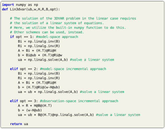
Listing 1.
Implementation of 3DVAR for with a linear observation operator.
3.2. Nonlinear Case
On the other hand, if is a nonlinear function, Equation (5) implies the solution of a system of nonlinear equations. Unlike linear systems, few algorithms are available to directly solve nonlinear systems and their convergence and stability are usually questionable. Alternatively, we can use Taylor series to expand around an initial estimate of , denoted as , where . The first-order approximation of can be written as
and Equation (5) can be approximated as
Thus, the correction to the initial guess of can be computed by solving the following system of linear equations
and a new guess of is estimated as , which is then plugged back into Equation (11) and the computations are repeated until convergence is reached. Python implementation of the 3DVAR in nonlinear observation operator is presented in Listing 2. Although we only present the first order approximation of , higher order expansions can be utilized for increased accuracy [27].
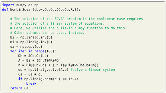
Listing 2.
Implementation of the 3DVAR for with a nonlinear observation operator, using
first-order approximation.
3.3. Example: Lorenz 63 System
The Lorenz 63 equations have been utilized as a toy problem in data assimilation studies, capturing some of the interesting mechanisms of weather systems. The three-equation model can be written as
where the values of are usually used to exhibit a chaotic behavior. If we like to put Equation (12) with the notations introduced in Section 2, we can write with , and with . A Python function describing the dynamics of the Lorenz 63 system is given in Listing 3.
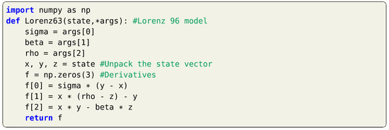
Listing 3.
A Python function for the Lorenz 63 dynamics.
Equation (12) describe the continuous-time evolution of the Lorenz system. In order to obtain the discrete-time mapping , a temporal integration scheme has to be applied. In Listing 4, one-step time integration functions are provided in Python using the first-order Euler and the fourth-order Runge–KuKutta schemes. Note that these functions requires a right-hand side function as input, this is mainly the continuous-time model (e.g., Listing 3).
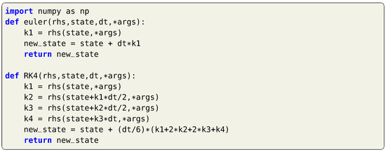
Listing 4.
Python functions for the time integration using the 1st Euler and the 4th
Runge–Kutta schemes.
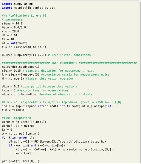
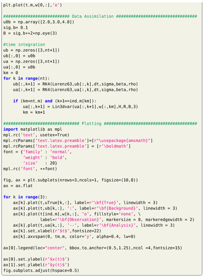
For twin experiment testing, we suppose a true initial condition of and measurements are collected each time units for a total time of 2. We suppose that we measure the full system state (i.e., , , and , where is the identity matrix). Measurements are considered to be contaminated by a white Gaussian noise with a zero mean and a covariance matrix . For simplicity, we let . For data assimilation testing, we assume that we begin with a perturbed initial condition of . Then, background state values are computed at by time integration of Equation (12) starting from this false initial condition. Observations at are assimilated to provide the analysis at . After that, background state values are computed at by time integration of Equation (12) starting from the analysis at , and so on. A sample implementation of the 3DVAR framework is presented in Listing 5, where a fixed background covariance matrix is assumed. Solution trajectories are presented in Figure 1 for a total time of 10, where observations are only available up to .
Listing 5.
Implementation of the 3DVAR for the Lorenz 63 system.
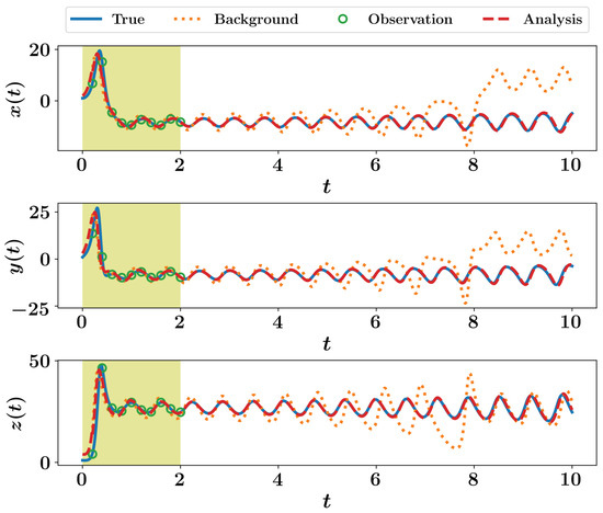
Figure 1.
Results of 3DVAR implementation for the Lorenz 63 system.
4. Four Dimensional Variational Data Assimilation
We highlighted in Section 3 that the 3DVAR can be referred to as a stationary case since the observations, background, and analysis all correspond to a fixed time instant. In other words, the optimization problem that minimizes Equation (4) takes place in the spatial state-space only. As an extension, the four dimensional variational data assimilation (4DVAR) aims to solve the optimization in both space and time, proving a non-stationary framework. In particular, the model’s dynamics are incorporated into the optimization problem to relate different points in time to each other. The cost functional for the 4DVAR Can be written as follows,
where is the measurement at time and defines the set of time instants where observations are available. Note that the argument of this cost functional is the initial condition . In other words, the purpose of the 4DVAR algorithm is to evaluate an initial state estimate, which if evolved in time, would produce a trajectory that is as close to the collected measurements as possible (weighted by the inverse of the covariance matrix of interfering noise). This is the place where the model’s dynamics comes into play to relate initial condition to future predictions when measurements are accessible. In other words, the values of are constrained by the underlying model. Instead of presenting the linear and nonlinear mappings separately, we will focus on the general case of both nonlinear model mapping and nonlinear observation operator, where simplification to linear cases should be straightforward.
In Equation (2), we introduced the one-step transition map and here, we can extend it to the k-step transition case by applying Equation (2) recursively as
where . Now, we consider a base trajectory given by for generated from an initial condition of . A perturbed trajectory ( for ) can be obtained by correcting the initial condition as and the difference between the perturbed and based trajectories can be written as
A first-order Taylor expansion of around can be given as follows
where is the Jacobian of the model , evaluated at , also known as the tangent linear operator. Note that and , thus . Similarly, we can expand around as follows,
where and . Consequently, , which can be generalized as,
with . It is customary to call Equation (18) as the perturbation equation, or the tangent linear system (TLS). Equation (18) can be related to by recursion as follows,
which can be short-handed as (please, notice the order of matrix multiplication and the subscript “”).
Now, we investigate the first order variation of the cost functional induced by the perturbation in the initial condition. This can be approximated as below,
Given that , then and Equation (20) can be rewritten as
By comparing Equations (19) and (21), the gradient of the cost functional can be approximated as
where . If we denote the time instants at which measurements are available as , Equation (23) can be expanded as
Now, defining a sequence of as below,
It can be verified that (assume some numbers and you can see this relation holds!). Therefore, in order to obtain the gradient of the cost functional, has to be computed, which depends on the evaluation of . In turn, the computation of requires and so on. Equation (25) is known as the first-order adjoint equation, as it implies the evaluation of sequence from to (i.e., reverse order).
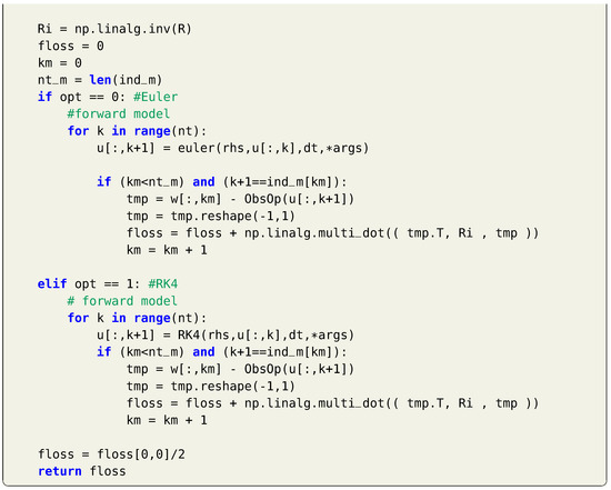
Therefore, the first-order approximation of the 4DVAR works as follows. Starting from a prior guess of the initial condition, the base trajectory is computed by solving the model forward in time until the final time corresponding the last observation point (i.e., ). Then, the value of is evaluated at final time. After that, is evolved backward in time using Equation (25) until is obtained. This value of the gradient is thus utilized to update the initial condition and a new base trajectory is generated. The solution of the 4DVAR problem requires the solution of the model dynamics forward in time and adjoint problem backward in time until to compute the gradient of the cost functional and update the initial condition. The process is thus repeated until convergence takes place. Listing 6 shows a sample function to compute the gradient of the cost functional corresponding to a base trajectory generated from a guess of the initial condition . We highlight that, in practice, the storage of the base trajectory as well as the sequence at every time instant might be overwhelming. However, we are not addressing such issues in these introductory tutorials to data assimilation techniques.
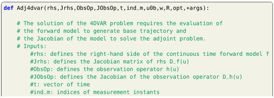
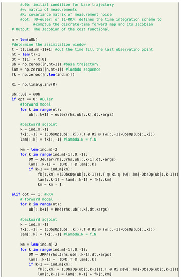
Listing 6.
Computation of the gradient of the cost functional with the 4DVAR using the first-order
adjoint algorithm.
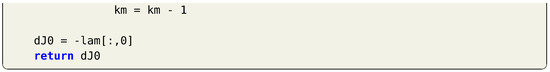
The gradient should be used in a minimization algorithm to update the initial condition for the next iteration. One simple algorithm is the simple gradient descent where an updated value of the initial state is computed as , where is some step parameter. This can be normalized as . The value of might be predefined, or more efficiently updated at each iteration using an additional optimization algorithm (e.g., line-search). For the sake of completeness, we present a line-search routine in Listing 7 using the Golden search algorithm. This is based on the definition of the cost functional in Listing 8.
Listing 7.
A line-search Python function using the Golden search method.
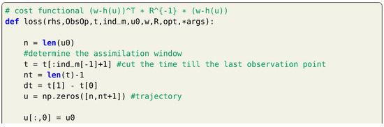
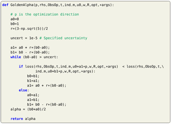
Listing 8.
Computation of the cost functional defined in Equation (13).
Example: Lorenz 63 System
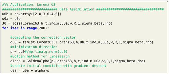
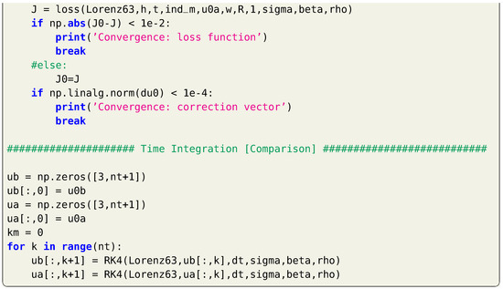
Similar to the 3DVAR demonstration, we apply the described 4DVAR using the first-order adjoint method on the Lorenz 63 system. We also begin with the same erroneous initial condition of and observations are collected each time units, contaminated with a Gaussian noise with diagonal covariance matrix defined as , where is the standard deviation for measurement noise. Moreover, we simply define a linear observation operator defined as , with a Jacobian of identity matrix. We utilize the simple gradient descent for minimizing the cost functional, equipped by a Golden search method for learning rate optimization. A maximum number of iterations is set to 1000, but we highlight that this is highly dependent on the adopted minimization algorithm as well as the line-search technique. In practice, the evaluation of each iteration might be too computationally expensive, so the number of iterations need to be as low as possible. We define two criteria for convergence, and iterations stop whenever any one of them is achieved. The first one is based on the change in the value of the cost or loss functional and the second one is based on the magnitude of its gradient. Extra criteria might be supplied as well.
Results for running Listing 9 is shown in Figure 2, where we can notice the significant improvement of predictions, compared to the background trajectories. Moreover, we highlight the correction to the initial conditions in Figure 2 which resulted in the analysis trajectory. This is opposed to the 3DVAR implementation, where correction is applied locally at measurements instants only as seen in Figure 1.
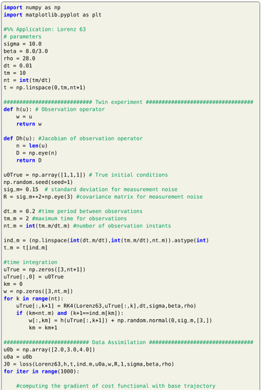
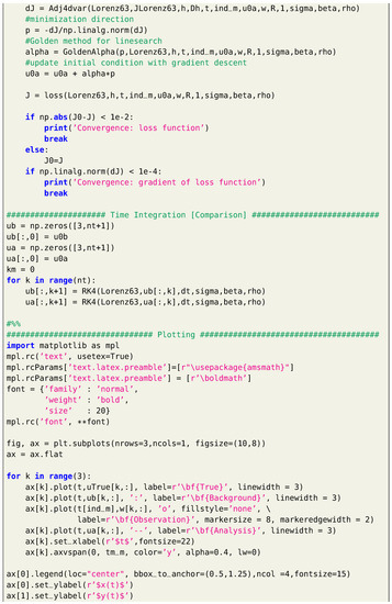

Listing 9.
Implementation of 4DVAR using the first-order adjoint method for the Lorenz 63 system.
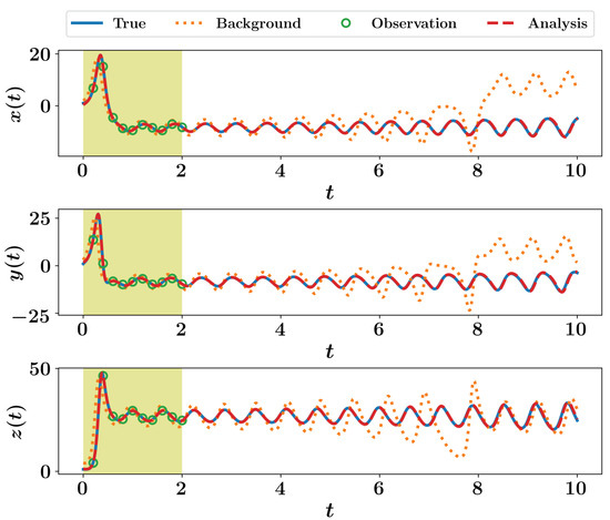
Figure 2.
Results of 4DVAR implementation for the Lorenz 63 system.
Before we move to other data assimilation techniques, we highlight a few remarks regarding our presentation of the 4DVAR
- In Listing 9, we utilize the gradient descent approach to minimize the cost function. Readers are encouraged to apply other optimization techniques (e.g., conjugate gradient) that achieve higher convergence rate.
- The determination of the learning rate can be further optimized using more efficient line-search methods, rather than the simple Golden search.
- The Lagrangian multiplier method can be applied to solve the 4DVAR problem instead of the adjoint method, similar results should be obtained.
- The presented algorithm relies on the definition of the cost functional given in Equation (13), based on the discrepancy between measurements and model’s predictions. When extra information is available, it can be incorporated into the cost functional. For instance, similar to Equation (4), a term that penalizes the correction magnitude can be added, weighted by the background covariance matrix. Furthermore, symmetries or other physical knowledge can be enforced as hard or weak constraints.
- The first-order adjoint algorithm requires the computation of the Jacobian of the discrete-time model map . This can be computed by plugging the model in a time integration scheme and rearranging everything to rewrite as explicit function of and differentiating with respect to components of . For Lorenz 63 and 1st Euler scheme, this can be an easy task. However, for a higher dimensional system and more accurate time integrators, this would be cumbersome. Instead, the chain rule can be utilized to compute as presented in Listing 10, which takes as input the right-hand side of the continuous-time dynamics (described in Listing 3 for Lorenz 63 system) as well as its Jacobian (given in Listing 11 for Lorenz 63).
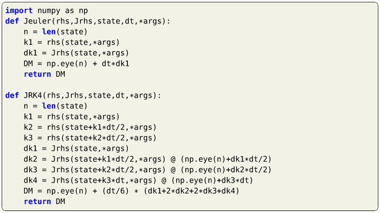 Listing 10. Python functions for computing the Jacobian of the discrete-time model map using the 1st Euler and the 4th Runge–Kutta schemes with chain rule.
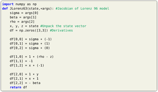 Listing 11. A Python function for the Jacobian of the continuous-time Lorenz 63 dynamics.
5. Forward Sensitivity Method
We have seen in Section 4 that the minimization of the cost functional via the 4DVAR algorithm requires the solution of the adjoint problem at each iteration, which incurs a significant computational burden for high dimensional systems. Alternatively, Lakshmivarahan and Lewis [13] proposed the forward sensitivity method (FSM) to derive an expression for the correction vector in terms of the forward sensitivity matrices [14]. In their development, simultaneous correction to the initial condition and the model parameters is treated. For conciseness and consistency with the methods introduced here, we only consider erroneous initial conditions and assume model parameters are perfectly known. Given the discrete-time model map in Equation (2), the forecast sensitivity at time to the initial conditions can be defined as follows,
where . Recall that the Jacobian of the model is defined by the matrix whose entry is defined as . We also define as the forward sensitivity matrix of with respect to initial state , where for . Thus, Equation (26) can be rewritten in matrix form as,
Equation (27) provides the dynamic evolution of the forward sensitivity matrix in a recursive manner, initialized by , that can be used to relate the prediction error at any time step to the initial condition.
Given the measurement at time , the forecast error is defined as the difference between the model forecast and measurements as
This is commonly called the innovation in DA terminology. The cost functional in Equation (13) can be rewritten as
With the assumption that the dynamical model is perfect (i.e., correctly encapsulates all the relevant processes) and the model parameters are known, the deterministic part of the forecast error can be attributed to the inaccuracy in the initial condition , defined as , where denotes the true initial conditions.
Considering a base trajectory for generated from the initial condition of , related to the corrected trajectory ( for ) obtained by correcting the initial condition as , we define the difference between both trajectories at any time as . We highlight that is a function of both the initial condition (with the model parameters being known), the first-order Taylor expansion of around the base trajectory can be written as , leading to the following relation
If we let the perturbed (corrected) trajectory to be the sought true trajectory, Equation (3) can be rewritten as
and a first order expansion of (neglecting the measurement noise) will be as follows,
and the forecast error at the base trajectory can be approximated as
Equations (30) and (33) can be combined to yield the following,
which relates the forecast error at any time and the discrepancy between the true and erroneous initial condition in a linear relationship. In order to account for all the time instants at which observations are available (), Equation (34) can be concatenated at different times and written as a linear system of equations as follows,
where the matrix and the vector are computed as,
Depending on the value of relative to n, Equation (35) can give rise to either an over-determined or an under-determined linear inverse problem. In either case, the inverse problem can be solved in a weighted least squares sense to find a first-order estimation of the optimal correction or perturbation to the initial condition , with being the weighting matrix, where is a block-diagonal matrix constructed as follows,
and the solution of Equation (35) can be written as for the over-determined case. This first order approximation progressively yields better results by repeating the entire process for multiple iterations until convergence with certain tolerance [13]. In essence, the FSM is an alternative to the 4DVAR algorithm, replacing the solution of the adjoint problem backward in time (i.e., Equation (25)), by the successive matrix evaluation in Equation (27). However, we highlight that in the 4DVAR approach, the actual forecast error is computed as while its first-order approximation is utilized in the FSM development. The duality between the two approaches is further discussed in [13].
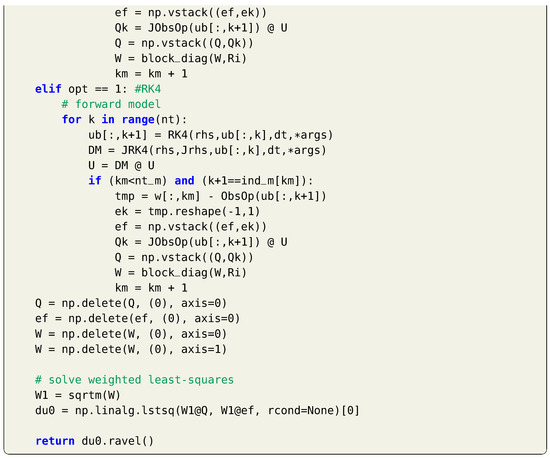
A Python implementation of the FSM approach is presented in Listing 12. We note that we solve the Equation (35) using the built-in numpy least-squares function. However, more efficient iterative schemes can be adopted in practice.
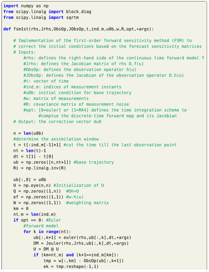
Listing 12.
Python function for computing the correction vector sing the forward sensitivity method with first-order approximation.
Example: Lorenz 63 System
We apply the described FSM to estimate the initial conditions for the Lorenz 63 system, using the same parameters and setup as described in Section 4. Sample code is presented in Listing 13. We highlight that instead of adding the correction vector directly to the base value , we multiply it with a learning rate to mitigate the effects of first-order approximations. We utilize the golden search method to update this learning rate at each iteration.
Listing 13.
Implementation of the FSM for the Lorenz 63 system.
Prediction results are provided in Figure 3, where we notice a large discrepancy at the estimated initial conditions. However, the predicted trajectory perfectly match the true one for the rest of the testing time window. This is largely affected by the nature of the Lorenz system itself and the attachment to its attractor. Furthermore, this can be partially attributed to the lack of background information and its contribution to the cost functional. Moreover, this can be highly improved by adding more observations close to the initial time since the correction vector is estimated based on the forecast error computed at observation times. Anyhow, we see that the analysis trajectory is significantly more accurate than the background one, with iterative first-order approximations of the forward sensitivity method, even for long time predictions.
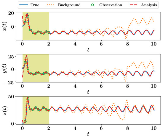
Figure 3.
Results of FSM implementation for the Lorenz 63 system.
6. Kalman Filtering
The idea behind Kalman filtering techniques is to propagate the mean as well as the covariance matrix of the system’s state sequentially in time. That is, in addition to providing an improved state estimate (i.e., the analysis), it also gives some information about the statistical properties of this state estimate. This is one main difference between Kalman filtering and variational methods, which often assumes a fixed (stationary) background covariance matrices. Kalman filters are also very popular in systems engineering, robotics, navigation, and control. Almost all modern control systems use the Kalman filter. It assisted the guidance of the Apollo 11 lunar module to the moon’s surface, and most probably will do the same for next generations of aircraft as well.
Although most application in fluid dynamics involve nonlinear systems, we first describe the standard Kalman filter developed for the linear dynamical system case with linear observation operator described as
where is a non-singular system matrix defining the underlying governing processes and describes the process noise (or model error). represents the measurement system with a measurement noise of .
As presented in Section 2, the true state is assumed to be a random variable with known mean and covariance matrix of . In Kalman filtering, we note that the covariance matrix evolves in time, and thus appears the subscript. We also assume that the process noise is unbiased with zero mean and a covariance matrix . That is and .
Thus, the goal of the filtering problem is to find a good estimate (analysis) of the true system’s state given a dynamical model a set of noisy observation collected at some time instants . The optimality of the estimate is defined as the one which minimizes . This filtering process generally consists of two steps: the forecast step and the data assimilation step.
The forecast step is performed using the predictable part of the given dynamical model starting from the best known information at time (denoted as to produce a forecast or background estimate . The difference between the background forecast and true state at can be written as follows,
where is the error estimate at , with zero mean and covariance matrix of .
The covariance matrix of the background estimate at can be evaluated as . Since, and are assumed to be uncorrelated (i.e., ), the background covariance matrix at can be computed as follows,
Now, with the forecast step, we have a background estimate at defined as with a covariance matrix . Then, measurements are collected at with a linear operator and measurement noise with zero mean a covariance matrix of . Thus, we would like to fuse these pieces of information to create an optimal unbiased estimate (analysis) with a covariance matrix . This can be defines as linear function of and as follows,
where is the innovation vector and is called the Kalman gain matrix. We highlight that Kalman gain matrix is defined in such a way to minimize . This can be written as [27]
resulting in an analysis covariance matrix defined as
where is the identity matrix. The resulting analysis is known as the best linear unbiased estimate (BLUE). We highlight that information at might correspond to the analysis (i.e., ) obtained from the last data assimilation implementation, or just from previous forecast if no other information is available. Thus, the Kalman filtering process can be summarized as follows,
where the inputs at are defined as
Listing 14 describes a basic Python implementation of the data assimilation step using the KF algorithm described before. Although efficient matrix inversion routines that benefit from specific matrix properties can be utilized, we use the standard built-in Numpy matrix inversion function.
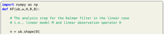
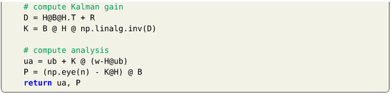
Listing 14.
Implementation of the KF with linear dynamics and observation operator.
Different forms for evaluating the Kalman gain and the covariance matrices are presented in literature. Some of them are favored for computational cost aspects, while others maintain desirable properties (e.g., symmetry and positive definiteness) for numerically stable implementation [27]. Since we are more interested in nonlinear dynamical models, we shall discuss extensions for standard Kalman filters to account for nonlinearity in the following sections.
7. Extended Kalman Filter
Instead of dealing with linear stochastic dynamics, we look at the nonlinear case with general (nonlinear) observation operator written as
The first challenge of applying Kalman filter for this system is the propagation of the background covariance matrix in the forecast step. The main clue behind the extended Kalman filter (EKF) to address this issue is to locally linearize by expanding it around the estimate at using the first-order Taylor series as follows,
where is the Jacobian (also known as the tangent linear operator) of the forward model evaluated at and defining the error estimate at , with zero mean and covariance matrix of . Thus, the difference between the background forecast and true state at can be written as follows,
Similar to the derivation in the linear case, with the assumption of uncorrelation between and , the background covariance matrix at can be computed as follows,
The next challenge regarding the analysis step is the computation of the Kalman gain in case of nonlinear observation operator. Again, is linearized using Talylor series expansion around (i.e., the background forecast) as follows,
where is the Jacobian of the observation operator h, computed with the forecast . The Kalman gain is thus computed using this first-order approximation of h as follows,
with an analysis estimate and analysis covariance matrix defined as
A summary of the EKF algorithm is described as follows,
and a Python implementation of the data assimilation step is presented in Listing 15.
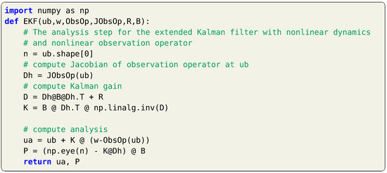
Listing 15.
Implementation of the (first-order) EKF with nonlinear dynamics and nonlinear
observation operator.
Example: Lorenz 63 System
The first-order approximation of the Kalman filter in nonlinear case, known as extended Kalman filter, is applied for the test case of Lorenz 63 system. The computation of model Jacobian is presented in Listing 10 and Listing 11 in Section 4. We use the same parameters and initial conditions for the twin experiment framework as before. The sequential implementation of the forecast and analysis steps is shown in Listing 16 and results are illustrated in Figure 4. We adopt the 4th order Runge–Kutta scheme for time integration. For demonstration purposes, we consider zero process noise (i.e., ). However, we have found that assuming non-zero process noise (e.g., ) yields better performance.
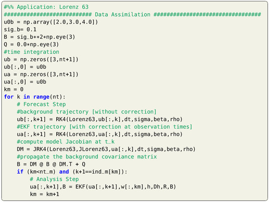
Listing 16.
Implementation of the EKF for the Lorenz 63 system.
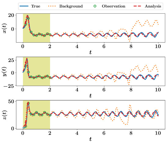
Figure 4.
EKF results for the Lorenz 63 system with the assumption of zero process noise.
8. Ensemble Kalman Filter
Despite the sound mathematical and theoretical foundation of Kalman filters (both linear and nonlinear cases), they are not widely utilized in geophysical sciences. The major bottleneck in the computational pipeline of Kalman filtering is the update of background covariance matrix. In typical implementation, the cost of this step is , where n is the size of the state vector. For systems governed by ordinary differential equations (ODES), n can be manageable (e.g., 3 in the Lorenz 63 model). However, fluid flows are often governed by partial differential equations. Thus, spatial discretization schemes (e.g., finite difference, finite volume, and finite element) are applied, resulting in a semi-discrete system of ODEs. In geophysical flow dynamics applications (e.g., weather forecast), a dimension of millions or even billions is not uncommon, which hinders the feasible implementation of standard Kalman filtering techniques.
Alternatively, reduced rank algorithms that provides low-order approximation of the covariance matrices are usually adopted. A very popular approach is the ensemble Kalman filter (EnKF), introduced by Evensen [17,28,29] based on the Monte Carlo estimation methods.
The main procedure for these methods is to create an ensemble of size N of the system state denoted as and apply the filtering algorithm to each member of the established ensemble. The statistical properties of the forecast and analysis are thus extracted from the ensemble using the standard Monte Carlo framework. In the previous discussions, the forecast (background) and analysis covariances are defined as follows,
Alternatively, those can be approximated by the ensemble covariances, given as
where the bar denotes the ensemble average defined as . Thus, an interpretation of EnKF is that the ensemble mean is the best estimate of the state and the spreading of the ensemble around the mean is a definition of the error in this estimate. A larger ensemble size N yields a better approximation of the state estimate and its covariance matrix. In the following, we describe the typical steps for applying the EnKF algorithm.
We begin by creating an initial ensemble at time drawn from the distribution , where represents our best-known estimate at . It can be verified that the ensemble mean and covariance converge to and as . Then, the forecast step is applied to each member of the enesemble as follows,
where is drawn from the multivariate Gaussian distribution with zero mean and covariance matrix of representing the process noise applied to each member. The sample mean of the forecast ensemble can be thus computed, along with the corresponding covaiance matrix as,
which provides an approximation for the background covariance at without actually propagating the covariance matrix, as is the case in standard Kalman filtering.
An enesmble of observations , also called virtual observations, is created assuming a Gaussian distribution with a mean equal to the actual observation and a covariance matrix . In other words, random Gaussian perturbations with zero mean and covariance matrix are added to the actual measurements to create perturbed measurements. The Kalman gain matrix can be computed as before (repeated here for completeness),
Then, the analysis step is applied for each member in the ensemble cloud as below,
and the analyzed estimate at is computed as the sample mean of the analysis ensemble along with its covariance matrix as follows,
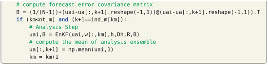
We observe that the EnKF algorithm provides approximations of the background and analysis covariance matrices, without the need to evaluate the computationally expensive propagation equations. This comes with the expense of having to evolve an ensemble of system’s states. However, the size of the ensemble N is usually smaller than the system’s dimension n. Moreover, with parallelization and high performance computing (HPC) frameworks, the forecast step can be distributed efficiently and computational speed-ups can be achieved. A summary of the EnKF algorithm is described as follows,
and Listing 17 provides a Python execution of the presented EnKF approach.
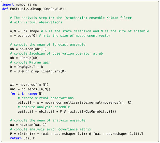
Listing 17.
Implementation of the EnKF with virtual observations.
We highlight a few remarks regarding the EnKF as below,
- Ensemble methods have gained significant popularity because of their simple conceptual formulation and relative ease of implementation. No optimization problem is required to be solved. They are considered non-intrusive in the sense that current solvers can be easily incorporated with minimal modification, as there is no need to derive model Jacobians or adjoint equations.
- The analysis ensemble can be used as initial ensemble for the next assimilation cycle (in which case, we need not compute ). Alternatively, new ensemble can be built, by sampling from multivariate Gaussian distribution with a mean of and covariance matrix of (i.e., using and in lieu of and , respectively).
- After virtual observations are made-up, an ensemble measurement error covariance matrix can be arbitrarily computed as an alternative to the actual one [17]. This is especially valuable when the actual measurement noise covariance matrix is poorly known.
- Perturbed observations are needed in EnKF derivation and guarantees that the posterior (analysis) covariance is not underestimated. For instance, in case of small corrections to the forecast, the traditional EnKF without virtual observations yields a error covariance that is about twice smaller than that is needed to match Kalman filter [30]. In other words, the use of virtual observations forces the ensemble posterior covariance to be the same as that of the standard Kalman filter in the limit of very large N. Thus, the same Kalman gain matrix relation is borrowed from standard Kalman filter.
- Instead of assuming virtual observations, alternative formulations of ensemble Kalman filters have been proposed in literature, giving a family of deterministic ensemble Kalman filter (DEnKF), as opposed to the aforementioned (stochastic) ensemble Kalman filer (EnKF). One such variant is briefly discussed in Section 8.1.
8.1. Deterministic Ensemble Kalman Filter
The use of an ensemble of perturbed observations in the EnKF leads to a match between the analysis error covariance and its theoretical value given by Kalman filter. However, this is in a statistical sense only when the ensemble size is large. Unfortunately, this perturbation introduces sampling error, which renders the filter suboptimal, particularly for small ensembles [31]. Alternative formulations that do not require virtual observations can be found in literature, including ensemble square root filters [31,32]. We focus here on a simple formulation proposed by Sakov and Oke [30] that maintains the numerical effectiveness and simplicity EnKF without the need to virtual observations, denoted as deterministic ensemble Kalman filter (DEnKF).
Without measurement perturbation, it can be derived that the resulting analysis error covariance matrix is given as follows,
With the definition of the Kalman gain, it can be seen that . Thus,
For small values of , this form converges to up to the quadratic term. It can be seen that this asymptotically match the theoretical value of analysis covariance matrix in standard Kalman filtering (i.e., ) by dividing the Kalman gain by two. Therefore, it can be argued that the DEnKF linearly recovers the theoretical analysis error covariance matrix. This is achieved by applying the analysis equation separately to the forecast mean with the Kalman gain matrix and ensemble of anomalies using half of the standard Kalman gain matrix. These steps are summarized as follows,
and Listing 18 provides a Python execution of the presented DEnKF approach. Note that the ensemble of observations is not created in this case, compared to the EnKF.
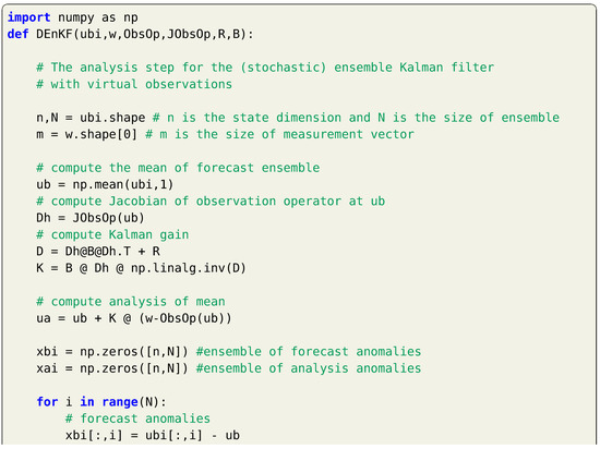
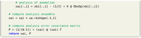
Listing 18.
Implementation of DEnKF without virtual observations.
8.2. Example: Lorenz 63 System
The same Lorenz 63 system is used to showcase the performance of both the EnKF and DEnKF. In Listing 19, we show the Python application of the EnKF algorithm. In general, the size of ensemble N is much smaller than the state dimension n for the implementation of EnKF to be computationally feasible. However, the state dimension in the Lorenz 63 is 3, and an ensemble of size 3 or less is trivial. The uncertainty in the covariance approximation via the Monte Carlo framework with such small ensemble becomes very high and resulting predictions are unreliable. There exists various approaches that help to increase the fidelity of small ensembles, including localization and inflation. In Section 9.2, we describe simple application of inflation factor and its impact with small ensembles. Here, we stick with the basic implementation with an ensemble size of 10 for both EnKF and DEnKF.
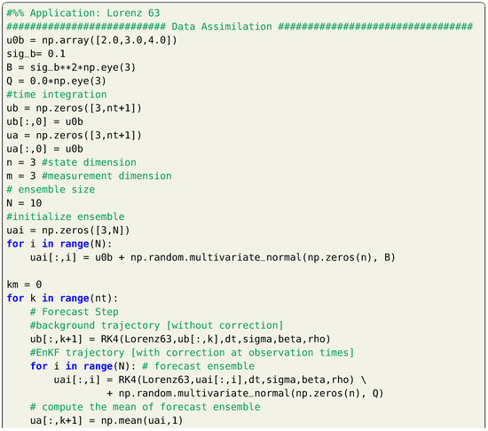
Listing 19.
Implementation of EnKF for the Lorenz 63 system.
Figure 5 shows the EnKF results for the Lorenz 63 system. We see that the analysis trajectory is close to the true one and more accurate than the background. Readers are encouraged to play with the codes to explore the effect of increasing or decreasing the ensemble size with different levels of noise. Furthermore, different observation operators can be defined (for instance, observe only 1 or 2 variables, or assume some nonlinear function ).
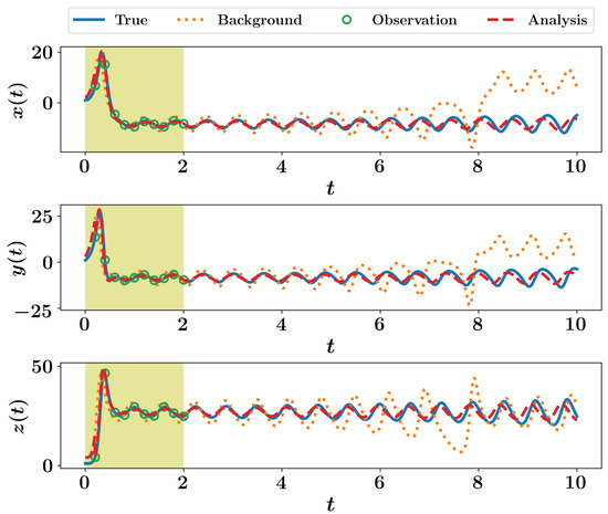
Figure 5.
EnKF results for the Lorenz 63 system with virtual observations.
For the sake of completeness, we also sketch the DEnKF predictions in Figure 6. The same implementation in Listing 19 can be adopted, but calling the DEnKF function framed in Listing 18 instead of EnKF. Although different approaches might give slightly dissimilar results, we are not trying to benchmark them in this introductory presentation since we are only showing very simple implementation, with idealized twin experiments.
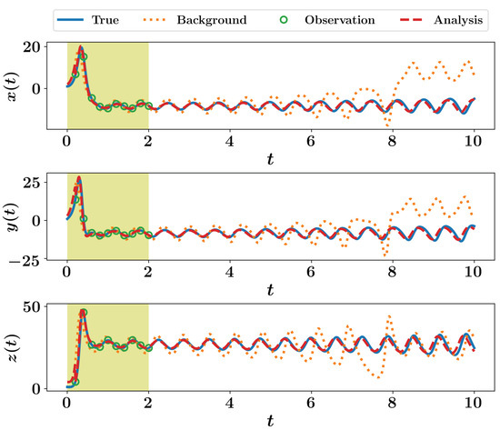
Figure 6.
DEnKF results for the Lorenz 63 system without virtual observations.
9. Applications
In this section, we gradually increase the complexity of the test cases using fluid dynamics applications. In Section 9.1, we slightly increase the dimensionality of the system from 3 (as in Lorenz 63 system) to 36 using the Lorenz 96 system and demonstrate the capability of DA algorithms to treat uncertainty in initial conditions. This is further extended in Section 9.2, where we show that DA can recover the hidden underlying processes and provide closure effects using the two-level variant of the Lorenz 96 model. We also introduce the utilization of an inflation factor and its impact to mitigate ensemble collapse and account for a slight under-representation of covariance due to the use of a small ensemble in EnKF and DEnKF. In Section 9.3, we illustrate the application of DA on systems governed by partial differential equations (PDEs) using the Kuramoto–Sivashinsky equation. We highlight that for each application, we only show results for a few selected algorithms and extensions to other approaches covered in this tutorial are left to readers as computer projects. We also emphasize that we are demonstrating the implementation and capabilities of the presented DA algorithms, not assessing their performance nor benchmarking different approaches against each other.
9.1. Lorenz 96 System
The Lorenz 96 model [33] is a system of ordinary differential equations that describes an arbitrary atmospheric quantity as it evolves on a circular array of sites, undergoing forcing, dissipation, and rotation invariant advection [34]. The Lorenz 96 dynamical model can be written as
where is the state of the system at the location and F represents a forcing constant. Periodicity is enforced by assuming that , , and . In the present study, we use , and defining a forcing term. In order to obtain a valid initial condition, we begin at using equilibrium conditions defined as ( for ) and adding a small perturbation to the 20th state variable as . Then, ODE integrator is run up to and solution at is treated at the true initial conditions for our twin experiment. We assume a background erroneous initial condition by contaminating the true one with Gaussian noise with zero mean and standard deviation of 1.
A total time window of 20 time units is considered, with a time step of and the RK4 schemes is adopted for time integration. Synthetic measurements are collected at every time unit (i.e., each 20 time integration steps) sampled at 9 equidistant locations (i.e., at ) from true trajectory assuming that sensors add a white noise with zero mean and a standard deviation of . We also assume a process noise drawn from a multivariate Gaussian distribution with zero mean and covariance matrix defined as . We first apply the EKF approach to correct the solution trajectory, which yields very good results as shown in Figure 7. For visualization, we only plot the time evolution of , , and . We see that the Lorenz 96 is sensitive to the initial conditions and small perturbation is sufficient to produce a very different trajectory (e.g., background solution).
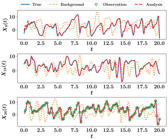
Figure 7.
EKF results for the Lorenz 96 system. The trajectories of , , and are shown.
The second approach to test is the stochastic version of EnKF. We create an ensemble of 50 members to approximate the covariance matrices. Results are depicted in Figure 8 for , , and . We highlight that observations appear only in the plot because observations are collected at (neither nor are measured). We highlight that, generally speaking, increasing the size of ensemble improves the predictions. However, this comes on the expense of the solution of the forward nonlinear model for each added member. Thus, a compromise between the accuracy and computational burden is in place.
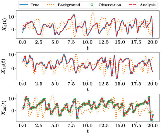
Figure 8.
EnKF results for the Lorenz 96 system using an ensemble of 50 members.
9.2. Two-Level Lorenz 96 System
In this section, we describe the two-level variant of the Lorenz 96 model proposed by Lorenz [33]. The two-level Lorenz 96 model can be written as
where Equation (62) represents the evolution of slow, high-amplitude variables , and Equation (63) provides the evolution of a coupled fast, low-amplitude variable . We use and in our computational experiments. We utilize and , which implies that the small scales fluctuate 10 times faster than the larger scales. Furthermore, the coupling coefficient h between two scales is equal to 1 and the forcing is set at to make both variables exhibit the chaotic behavior.
We utilize the fourth-order Runge–Kutta numerical scheme with a time step for temporal integration of the Lorenz 96 model. We apply the periodic boundary condition for the slow variables, i.e., . The fast variables are extended by letting , , and . The physical initial condition is computed by starting with an equilibrium condition at time for slow variables. The equilibrium condition for slow variables is for . We perturb the equilibrium solution for the 18th state variable as . At the time , the fast variables are assigned with random numbers between to . We integrate a two-level Lorenz 96 model by solving both Equations (62) and (63) in a coupled manner up to time . The solution at time represent the true initial condition. For our twin experiment, we obtain observations by adding noise drawn from the Gaussian distribution with zero mean and . We assume that observations are sparse in space and are collected at every 10th time step.
The motivation behind this example is to demonstrate how covariance inflation can be utilized to account for the model error. Usually the imperfections in the forecast model is taken into account by adding a Gaussian noise to the forecast model. Another method to account for model error is covarinace inflation. It also helps in alleviating the effect finite number of ensemble members in practical data assimilation and addresses the problem of covariance underestimation in the EnKF algorithm. We use the multiplicative inflation [35] where the ensemble members are pushed away from the ensemble mean by a given inflation factor and mathematically it can be expressed as
where is the inflation factor. The inflation factor can be a constant scalar over the entire domain at all time step or it can space and time dependent.
In this example, we discard parameterizations of fast variables in the forecast model. The forecast model for two-level Lorenz system with no parameterizations is equivalent to setting the coupling coefficient in Equation (62) and it reduces to one-level Lorenz 96 model as presented in Section 9.1. We note here that the observations used for data assimilation are obtained by solving a two-level Lorenz 96 model in a coupled manner (i.e., without discarding fast-variables). Therefore, the effect of unresolved scales is embedded in observations. The parameterization of fast variables (i.e., term in Equation (62)) can be considered as an added noise to the true state of the system for a one-level Lorenz 96 model. Figure 9 displays the RMSE for a two-level Lorenz system when 18 observations are used for DA with different number of ensemble members and inflation factors for EnKF and DEnKF algorithms. Figure 10 shows the full state trajectory of two-level Lorenz system corresponding to minimum RMSE, which is obtained with 50 ensemble members and inflation factor for the EnKF algorithm. The parameters corresponding to minimum RMSE for the DEnKF algorithm are 45 ensemble members and .
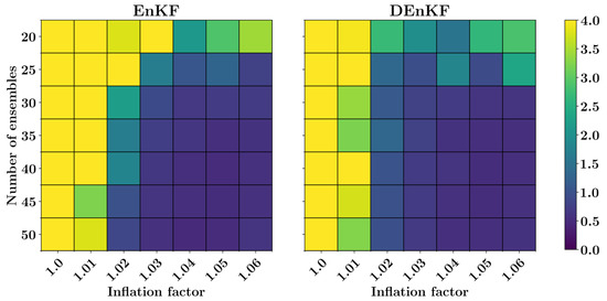
Figure 9.
RMSE for a two-level Lorenz model for different combinations of number of ensembles and inflation factor.
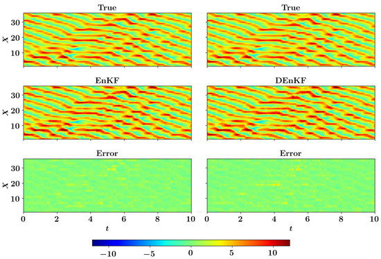
Figure 10.
Full state trajectory of the multiscale Lorenz 96 model with no parameterizations in the forecast model. The EnKF algorithm uses the inflation factor and and the DEnKF uses the inflation factor and . The observation data for both EnKF an DEnKF algorithm is obtained by adding measurement noise to the exact solution of the two-level Lorenz 96 system.
9.3. Kuramato Sivashinsky
In this section, we describe the Kuramoto–Sivashinsky (K-S) equation derived by Kuramoto [36], which is used as a turbulence model for different flows. The one-dimensional K-S equation can be written as
where is the viscosity coefficient. The K-S equation is characterized by the second-order unstable diffusion term responsible for an instability at large scales, the fourth-order stabilizing viscous term that provides damping at small scales, and a quadratic nonlinear term which transfers energy between large and small scales. We use the computational domain extending from 0 to L, i.e., and time . We impose the Dirichlet and Neumann boundary conditions as given below
We spatially discretize the domain with the grid size , where n is the degrees of freedom. We set and for our numerical experiments. The state of the system at discretized grid is denoted as for . Using the second-order finite difference discretization, the discretized K-S equation can be written as
The first term on the right hand side is computed by utilizing ghost nodes and the Neumann boundary condition is assigned for ghost points. We impose and using the second-order discretization for Equation (67) at boundary points and , respectively.
We use the fourth-order Runge–Kutta scheme for time integration with a time step . To generate an initial condition for the forward run we start with an equilibrium condition at time and integrate up to time . The equilibrium condition for the model is for . Once the true initial condition is generated, we run the forward solver up to time . We test the prediction capability of sequential data assimilation algorithms for forecast up to . The K-S equation exhibits different levels of chaotic behavior depending on the value of viscosity coefficient . The chaos depends upon the bifurcation parameter . We utilize which represent the less chaotic behaviour. The observations for twin experiments are obtained by adding some noise to the true state of the system to account for experimental uncertainties and measurement errors. The observations are also sparse in time, meaning that the time interval between two observations can be different from the time step of the forecast model. For our twin experiments, we assume that observations are recorded at every 10th time step of the model for . Therefore, the time difference between two observations is for the K-S equation. We present results for the EnKF algorithm with three sets of observations. The first set of observations is very sparse with only 12.5% of the full state of the system. The first set utilizes observations for states . In a second set of observations we employ observations at for the assimilation. The third set of observations consists of 50% of the full state of the system, i.e., observations at states for the assimilation. We apply and as the variance of observation noise and initial condition uncertainty, respectively.
In Figure 11, we present the time evolution of selected states for three different number of observations included in the assimilation of the EnKF algorithm. There is an excellent agreement between true and assimilated states and , for which observations are not present. We also provide the full state trajectory of the K-S equation in Figure 12. The results obtained clearly indicate that the EnKF algorithm is able to determine the correct state trajectory even when the observation data are very sparse, i.e., . With an increase in the number of observations, the prediction of the full state trajectory gets smoother, and almost the exact state is recovered with 50% observations.
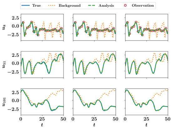
Figure 11.
Selected trajectories of the Kuramoto–Sivashinsky model () with the analysis performed by the ensemble Kalman filter (EnKF) using observations from (left), (middle), and (right) state variables at every 10 time steps.
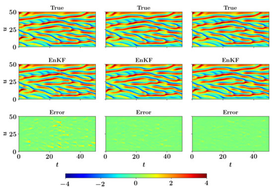
Figure 12.
Full state trajectory of the Kuramoto–Sivashinsky model () with the analysis performed by the ensemble Kalman filter (EnKF) using observations from (left), (middle), and (right) state variables at every 10 time steps.
9.4. Quasi-Geostrophic (QG) Ocean Circulation Model
We consider a simple single-layer QG model to illustrate the application of sequential data assimilation for two-dimensional flows. Specifically, we use the deterministic ensemble Kalman filter (DenKF) algorithm discussed in Section 8.1 to improve the prediction of the single-layer QG model. The wind-driven oceanic flows exhibit a vast range of spatio-temporal scales and modeling of these scales with all the relevant physics has always been challenging. The barotropic vorticity equation (BVE) with various dissipative and forcing terms is one of the most commonly used models for geostrophic flows [37,38]. The dimensionless vorticity-streamfunction formulation for the BVE [39] with forcing and dissipative terms can be written as
where is the vorticity, is the streamfunction, is the standard two-dimensional Laplacian operator, Re is the Reynolds number, and is the Rossby number. The kinematic relation between vorticity and streamfunction is given by the following Poisson equation
The nonlinear convection term is given by the Jacobian as follows
The computational domain for the QG model is and is discretized using grid resolution. Therefore, the QG model has the dimension of about . We utilize the homogeneous Dirichlet boundary condition for the vorticity and streamfunction at all boundaries. The vorticity and streamfunction is initialized from quiescent state, i.e., . The QG model is numerically solved by discretizing Equation (69) using second-order finite difference scheme. The nonlinear Jacobian term is discretized with the energy-conserving Arakawa [40] numerical scheme. A third-order total-variation-diminishing Runge–Kutta scheme is used for the temporal integration and a fast sine transform Poisson solver is utilized to update streamfunction from the vorticity [41]. For the physical parameters, we use values of and .
The QG model is integrated with a constant time step of from time to to generate the true initial condition at final time . Then the data assimilation is conducted from time to with observations getting assimilated at every tenth time step. The synthetic observations are generated by sampling vorticity field on 16 equidistant points in x and y directions respectively and then adding the Gaussian noise, i.e., , where . We set the observation noise variance at . The typical vorticity and streamfunction field along with the locations of measurements are shown in Figure 13.
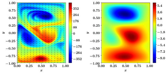
Figure 13.
A Typical vorticity (left) and streamfunction (right) field for the single-layer QG model. The dots shows the locations of observations.
We employ 20 ensemble members for the DEnKF algorithm. The initialization of the ensemble members is an important step to get accurate prediction with any type of the EnKF algorithm. We initialize different ensemble members by randomly selecting the vorticity field snapshots between time to . The other methods such as adding a random perturbation from the Gaussian distribution to the true initial condition can also be adopted. Figure 14 displays the vorticity field and the predicted vorticity field at three different time instances along with the difference (error) between the two. We can see that the true and analysis field are similar at all time instances and the magnitude of error is also small. We recall that we observe only around 2% of the system (i.e., observations at locations). With more observations, the quality of the results can be further improved.
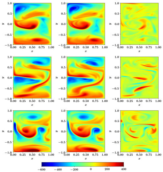
Figure 14.
Snapshots of the true vorticity field (left), analysis estimate of the DEnKF algorithm (middle), and the difference (error) between the two fields (right) obtained for a particular run of the single-layer QG model. The snapshots of vorticity field are plotted at (from top to bottom).
10. Concluding Remarks
In this tutorial paper, we provided a 101 introduction to common data assimilation techniques. In particular, we briefly covered the relevant mathematical foundation and the algorithmic steps for three dimensional variational (3DVAR), four dimensional variational (4DVAR), forward sensitivity method (FSM), and Kalman filtering approaches. Since it is considered as a first exposure to DA, we focused on the simplest implementations that anybody can easily follow. For example, to treat nonlinearity (e.g., in 3DVAR, 4DVAR, FSM and EKF), we only presented the first order Taylor expansions. We demonstrated the execution of the covered approaches with a series of Python modules that can be linked to each other easily. Again, we preferred to keep our codes as concise and simple as possible, even if it comes on the expense of computational efficiency. The Python codes used to generate this tutorial are publicly available through our GitHub repository https://github.com/Shady-Ahmed/PyDA.
Since it is introductory exploration, we should admit that we have bypassed a few important analyses and shortcut some key derivations. Interested readers are referred to well-established textbooks that offer in-depth discussions about various DA techniques [14,27,29,42,43,44,45,46,47]. Likewise, more advanced topics such as the particle filters [48], maximum likelihood ensemble filters [49,50], optimal sensor placement [51,52], higher-order analysis of variational methods [53], or hybrid methods [54,55,56,57,58,59] are omitted in our current presentation.
Author Contributions
Data curation, S.E.A., S.P., and O.S.; Supervision, O.S.; Writing—original draft, S.E.A., and S.P.; and Writing—review and editing, S.E.A., S.P., and O.S. All authors have read and agreed to the published version of the manuscript.
Funding
This material is based upon work supported by the U.S. Department of Energy, Office of Science, Office of Advanced Scientific Computing Research under Award Number DE-SC0019290. Omer San gratefully acknowledges their support. Disclaimer: This report was prepared as an account of work sponsored by an agency of the United States Government. Neither the United States Government nor any agency thereof, nor any of their employees, makes any warranty, express or implied, or assumes any legal liability or responsibility for the accuracy, completeness, or usefulness of any information, apparatus, product, or process disclosed, or represents that its use would not infringe privately owned rights. Reference herein to any specific commercial product, process, or service by trade name, trademark, manufacturer, or otherwise does not necessarily constitute or imply its endorsement, recommendation, or favoring by the United States Government or any agency thereof. The views and opinions of authors expressed herein do not necessarily state or reflect those of the United States Government or any agency thereof.
Acknowledgments
We thank Sivaramakrishnan Lakshmivarahan for his insightful comments as well as his archival NPTEL lectures [60] on dynamic data assimilation that greatly helped us in developing the PyDA module. Special thanks go to Ionel Michael Navon for providing his lecture notes on data assimilation.
Conflicts of Interest
The authors declare no conflict of interest.
References
- Navon, I.M. Data assimilation for numerical weather prediction: A review. In Data Assimilation for Atmospheric, Oceanic and Hydrologic Applications; Springer: Berlin/Heidelberg, Germany, 2009; pp. 21–65. [Google Scholar]
- Blum, J.; Le Dimet, F.X.; Navon, I.M. Data assimilation for geophysical fluids. Handb. Numer. Anal. 2009, 14, 385–441. [Google Scholar]
- Le Dimet, F.X.; Navon, I.M.; Ştefănescu, R. Variational data assimilation: Optimization and optimal control. In Data Assimilation for Atmospheric, Oceanic and Hydrologic Applications (Vol. III); Springer: Berlin/Heidelberg, Germany, 2017; pp. 1–53. [Google Scholar]
- Attia, A.; Sandu, A. DATeS: A highly extensible data assimilation testing suite v1.0. Geosci. Model Dev. 2019, 12, 629–649. [Google Scholar] [CrossRef]
- Lorenc, A.C. Analysis methods for numerical weather prediction. Q. J. R. Meteorol. Soc. 1986, 112, 1177–1194. [Google Scholar] [CrossRef]
- Parrish, D.F.; Derber, J.C. The National Meteorological Center’s spectral statistical-interpolation analysis system. Mon. Weather Rev. 1992, 120, 1747–1763. [Google Scholar] [CrossRef]
- Courtier, P. Dual formulation of four-dimensional variational assimilation. Q. J. R. Meteorol. Soc. 1997, 123, 2449–2461. [Google Scholar] [CrossRef]
- Rabier, F.; Järvinen, H.; Klinker, E.; Mahfouf, J.F.; Simmons, A. The ECMWF operational implementation of four-dimensional variational assimilation. I: Experimental results with simplified physics. Q. J. R. Meteorol. Soc. 2000, 126, 1143–1170. [Google Scholar] [CrossRef]
- Elbern, H.; Schmidt, H.; Talagrand, O.; Ebel, A. 4D-variational data assimilation with an adjoint air quality model for emission analysis. Environ. Model. Softw. 2000, 15, 539–548. [Google Scholar] [CrossRef]
- Courtier, P.; Thépaut, J.N.; Hollingsworth, A. A strategy for operational implementation of 4D-Var, using an incremental approach. Q. J. R. Meteorol. Soc. 1994, 120, 1367–1387. [Google Scholar] [CrossRef]
- Lorenc, A.C.; Rawlins, F. Why does 4D-Var beat 3D-Var? Q. J. R. Meteorol. Soc. 2005, 131, 3247–3257. [Google Scholar] [CrossRef]
- Gauthier, P.; Tanguay, M.; Laroche, S.; Pellerin, S.; Morneau, J. Extension of 3DVAR to 4DVAR: Implementation of 4DVAR at the Meteorological Service of Canada. Mon. Weather Rev. 2007, 135, 2339–2354. [Google Scholar] [CrossRef]
- Lakshmivarahan, S.; Lewis, J.M. Forward sensitivity approach to dynamic data assimilation. Adv. Meteorol. 2010, 2010, 375615. [Google Scholar] [CrossRef]
- Lakshmivarahan, S.; Lewis, J.M.; Jabrzemski, R. Forecast Error Correction Using Dynamic Data Assimilation; Springer: Cham, Switzerland, 2017. [Google Scholar]
- Houtekamer, P.L.; Mitchell, H.L. Data assimilation using an ensemble Kalman filter technique. Mon. Weather Rev. 1998, 126, 796–811. [Google Scholar] [CrossRef]
- Burgers, G.; Jan van Leeuwen, P.; Evensen, G. Analysis scheme in the ensemble Kalman filter. Mon. Weather Rev. 1998, 126, 1719–1724. [Google Scholar] [CrossRef]
- Evensen, G. The ensemble Kalman filter: Theoretical formulation and practical implementation. Ocean. Dyn. 2003, 53, 343–367. [Google Scholar] [CrossRef]
- Houtekamer, P.L.; Mitchell, H.L. A sequential ensemble Kalman filter for atmospheric data assimilation. Mon. Weather Rev. 2001, 129, 123–137. [Google Scholar] [CrossRef]
- Houtekamer, P.L.; Mitchell, H.L. Ensemble kalman filtering. Q. J. R. Meteorol. Soc. 2005, 131, 3269–3289. [Google Scholar] [CrossRef]
- Treebushny, D.; Madsen, H. A new reduced rank square root Kalman filter for data assimilation in mathematical models. In Proceedings of the International Conference on Computational Science, Melbourne, Australia, 2 June 2003; Springer: Berlin/Heidelberg, Germany, 2003; pp. 482–491. [Google Scholar]
- Buehner, M.; Malanotte-Rizzoli, P. Reduced-rank Kalman filters applied to an idealized model of the wind-driven ocean circulation. J. Geophys. Res. Ocean. 2003, 108. [Google Scholar] [CrossRef]
- Lakshmivarahan, S.; Stensrud, D.J. Ensemble Kalman filter. IEEE Control. Syst. Mag. 2009, 29, 34–46. [Google Scholar]
- Apte, A.; Hairer, M.; Stuart, A.; Voss, J. Sampling the posterior: An approach to non-Gaussian data assimilation. Phys. Nonlinear Phenom. 2007, 230, 50–64. [Google Scholar] [CrossRef]
- Bocquet, M.; Pires, C.A.; Wu, L. Beyond Gaussian statistical modeling in geophysical data assimilation. Mon. Weather Rev. 2010, 138, 2997–3023. [Google Scholar] [CrossRef]
- Vetra-Carvalho, S.; Van Leeuwen, P.J.; Nerger, L.; Barth, A.; Altaf, M.U.; Brasseur, P.; Kirchgessner, P.; Beckers, J.M. State-of-the-art stochastic data assimilation methods for high-dimensional non-Gaussian problems. Tellus Dyn. Meteorol. Oceanogr. 2018, 70, 1–43. [Google Scholar] [CrossRef]
- Attia, A.; Moosavi, A.; Sandu, A. Cluster sampling filters for non-Gaussian data assimilation. Atmosphere 2018, 9, 213. [Google Scholar] [CrossRef]
- Lewis, J.M.; Lakshmivarahan, S.; Dhall, S. Dynamic Data Assimilation: A Least Squares Approach; Cambridge University Press: Cambridge, UK, 2006; Volume 104. [Google Scholar]
- Evensen, G. Sequential data assimilation with a nonlinear quasi-geostrophic model using Monte Carlo methods to forecast error statistics. J. Geophys. Res. Ocean. 1994, 99, 10143–10162. [Google Scholar] [CrossRef]
- Evensen, G. Data Assimilation: The Ensemble Kalman Filter; Springer: Berlin/Heidelberg, Germany, 2009. [Google Scholar]
- Sakov, P.; Oke, P.R. A deterministic formulation of the ensemble Kalman filter: An alternative to ensemble square root filters. Tellus Dyn. Meteorol. Oceanogr. 2008, 60, 361–371. [Google Scholar] [CrossRef]
- Whitaker, J.S.; Hamill, T.M. Ensemble data assimilation without perturbed observations. Mon. Weather Rev. 2002, 130, 1913–1924. [Google Scholar] [CrossRef]
- Tippett, M.K.; Anderson, J.L.; Bishop, C.H.; Hamill, T.M.; Whitaker, J.S. Ensemble square root filters. Mon. Weather Rev. 2003, 131, 1485–1490. [Google Scholar] [CrossRef]
- Lorenz, E.N. Predictability: A problem partly solved. In Proceedings of the Seminar on Predictability, Reading, UK, 9–11 September 1996; Volume 1. [Google Scholar]
- Kerin, J.; Engler, H. On the Lorenz’96 Model and Some Generalizations. arXiv 2020, arXiv:2005.07767. [Google Scholar]
- Anderson, J.L.; Anderson, S.L. A Monte Carlo implementation of the nonlinear filtering problem to produce ensemble assimilations and forecasts. Mon. Weather Rev. 1999, 127, 2741–2758. [Google Scholar] [CrossRef]
- Kuramoto, Y. Diffusion-induced chaos in reaction systems. Prog. Theor. Phys. Suppl. 1978, 64, 346–367. [Google Scholar] [CrossRef]
- Majda, A.; Wang, X. Nonlinear Dynamics and Statistical Theories for basic Geophysical Flows; Cambridge University Press: New York, NY, USA, 2006. [Google Scholar]
- Greatbatch, R.J.; Nadiga, B.T. Four-gyre circulation in a barotropic model with double-gyre wind forcing. J. Phys. Oceanogr. 2000, 30, 1461–1471. [Google Scholar] [CrossRef]
- San, O.; Staples, A.E.; Wang, Z.; Iliescu, T. Approximate deconvolution large eddy simulation of a barotropic ocean circulation model. Ocean. Model. 2011, 40, 120–132. [Google Scholar] [CrossRef]
- Arakawa, A. Computational design for long-term numerical integration of the equations of fluid motion: Two-dimensional incompressible flow. Part I. J. Comput. Phys. 1997, 135, 103–114. [Google Scholar] [CrossRef]
- Press, W.H.; Flannery, B.P.; Teukolsky, S.A.; Vetterling, W.T. Numerical Recipes; Cambridge University Press: New York, NY, USA, 1989. [Google Scholar]
- Cacuci, D.G.; Navon, I.M.; Ionescu-Bujor, M. Computational Methods for Data Evaluation and Assimilation; CRC Press: New York, NY, USA, 2013. [Google Scholar]
- Kalnay, E. Atmospheric Modeling, Data Assimilation and Predictability; Cambridge University Press: New York, NY, USA, 2003. [Google Scholar]
- Law, K.; Stuart, A.; Zygalakis, K. Data Assimilation: A Mathematical Introduction; Springer: Cham, Switzerland, 2015. [Google Scholar]
- Asch, M.; Bocquet, M.; Nodet, M. Data Assimilation: Methods, Algorithms, and Applications; SIAM: Philadelphia, PA, USA, 2016. [Google Scholar]
- Simon, D. Optimal State Estimation: Kalman, H Infinity, and Nonlinear Approaches; John Wiley & Sons: Hoboken, NJ, USA, 2006. [Google Scholar]
- Labbe, R. Kalman and bayesian filters in Python. Chap 2014, 7, 246. [Google Scholar]
- Van Leeuwen, P.J.; Künsch, H.R.; Nerger, L.; Potthast, R.; Reich, S. Particle filters for high-dimensional geoscience applications: A review. Q. J. R. Meteorol. Soc. 2019, 145, 2335–2365. [Google Scholar] [CrossRef] [PubMed]
- Zupanski, M. Maximum likelihood ensemble filter: Theoretical aspects. Mon. Weather Rev. 2005, 133, 1710–1726. [Google Scholar] [CrossRef]
- Zupanski, M.; Navon, I.M.; Zupanski, D. The Maximum Likelihood Ensemble Filter as a non-differentiable minimization algorithm. Q. J. R. Meteorol. Soc. 2008, 134, 1039–1050. [Google Scholar] [CrossRef]
- Kang, W.; Xu, L. Optimal placement of mobile sensors for data assimilations. Tellus Dyn. Meteorol. Oceanogr. 2012, 64, 17133. [Google Scholar] [CrossRef]
- Mons, V.; Chassaing, J.C.; Sagaut, P. Optimal sensor placement for variational data assimilation of unsteady flows past a rotationally oscillating cylinder. J. Fluid Mech. 2017, 823, 230–277. [Google Scholar] [CrossRef]
- Le Dimet, F.X.; Navon, I.M.; Daescu, D.N. Second-order information in data assimilation. Mon. Weather Rev. 2002, 130, 629–648. [Google Scholar] [CrossRef]
- Lorenc, A.C.; Bowler, N.E.; Clayton, A.M.; Pring, S.R.; Fairbairn, D. Comparison of hybrid-4DEnVar and hybrid-4DVar data assimilation methods for global NWP. Mon. Weather Rev. 2015, 143, 212–229. [Google Scholar] [CrossRef]
- Desroziers, G.; Camino, J.T.; Berre, L. 4DEnVar: Link with 4D state formulation of variational assimilation and different possible implementations. Q. J. R. Meteorol. Soc. 2014, 140, 2097–2110. [Google Scholar] [CrossRef]
- Wang, X.; Barker, D.M.; Snyder, C.; Hamill, T.M. A hybrid ETKF–3DVAR data assimilation scheme for the WRF model. Part I: Observing system simulation experiment. Mon. Weather Rev. 2008, 136, 5116–5131. [Google Scholar] [CrossRef]
- Buehner, M.; Morneau, J.; Charette, C. Four-dimensional ensemble-variational data assimilation for global deterministic weather prediction. Nonlinear Process. Geophys. 2013, 20, 669–682. [Google Scholar] [CrossRef]
- Kleist, D.T.; Ide, K. An OSSE-based evaluation of hybrid variational-ensemble data assimilation for the NCEP GFS. Part I: System description and 3D-hybrid results. Mon. Weather Rev. 2015, 143, 433–451. [Google Scholar] [CrossRef]
- Kleist, D.T.; Ide, K. An OSSE-based evaluation of hybrid variational-ensemble data assimilation for the NCEP GFS. Part II: 4DEnVar and hybrid variants. Mon. Weather Rev. 2015, 143, 452–470. [Google Scholar] [CrossRef]
- Lakshmivarahan, S. Video Lectures on Dynamic Data Assimilation; NPTEL Program; IIT Madras: Chennai, India, 2016; Available online: https://nptel.ac.in/courses/111/106/111106082/ (accessed on 28 November 2020).


Publisher’s Note: MDPI stays neutral with regard to jurisdictional claims in published maps and institutional affiliations. |
© 2020 by the authors. Licensee MDPI, Basel, Switzerland. This article is an open access article distributed under the terms and conditions of the Creative Commons Attribution (CC BY) license (http://creativecommons.org/licenses/by/4.0/).