The Influence of Inflow Swirl on Cavitating and Mixing Processes in a Venturi Tube

Abstract

A study of the mixing flows (Schmidt number = 10${}^3$) in a cavitating Venturi tube that feature linear and swirling flows is presented in this paper. The Large Eddy Simulation (LES) turbulence model, the Schnerr–Sauer cavitation model, and the mixture multiphase model, as implemented in the commercial CFD ANSYS FLUENT 16.2, were employed. The main emphasis is spending on the influence of different inlet swirling ratios on the generation of cavitation and mixing behaviors in a Venturi tube. Four different inflow regimes were investigated for the Reynolds number Re = 19,044, 19,250, 19,622, 21,276: zero swirl, 15% swirl, 25% swirl and 50% swirl velocity relative to the transverse inflow velocity, respectively. The computed velocity and pressure profiles were shown in good agreement with the experiment data from the literature. The predicted results indicate that the imposed swirl flow moves the cavitation bubbles away from throat surfaces toward the throat axis. The rapid mixing between two volumetric components is promoted in the divergent section when the intense swirl is introduced. Additionally, the increase in the swirl ratio from 0.15 to 0.5 leads to a linear increase in the static pressure drop and a nonlinear increase in the vapor production. The reduction in the fluid viscosity ratio from $\frac{{\mu }_2}{{\mu }_1}=10$ to $\frac{{\mu }_2}{{\mu }_1}=1$ generates a high cavitation intensity in the throat of the Venturi tube. However, the changes in the pressure drop and vapor volume fraction are significantly small of pure water flow.

1. Introduction

A cavitating Venturi tube is a micro- and nano-sized bubble generator which consists of three sequential parts: a convergent section, a throat section, and a divergent section. Due to their simple structure, the cavitating Venturi tubes have been widely used for industrial applications, such as wastewater treatment, oil and gas industrial, mineral processing, and mixing of fluids. By passing the liquid through the Venturi tubes, the local pressure drops down to the saturation vapor pressure due to a decrease in the throat area, which leads to the formation of cavitation bubbles at the throat and divergent sections. Subsequently, a highly turbulent flow is generated in this region. Under the action of the high degree of turbulence, the Venturi tube is employed as a passive mixer to achieve better mixing performance, such as when mixing liquid–liquid components [1,2] and gas–gas components [3,4]. Effective rapid mixing of various fluids can reduce the time required for reaction and improve reaction efficiency in industrial operations. The major advantages of using a Venturi mixer are the high level of mixing efficiency, low energy requirement and short mixing length [2]. Therefore, much attention has been paid to the Venturi tubes in the past decades and numerous investigations in predicting the cavitating and mixing processing have been conducted.

There are many geometrical and operational parameters that have significant impact on the performance of cavitation or mixing in a Venturi tube, such as the throat length, the throat diameter, the convergent and divergent angles, the inlet and outlet pressures, and the injection of gas or solid particles [5,6,7,8,9,10]. Any change made to one or several of the above-mentioned parameters will result in a drastic change in the mixing and mass transfer rate. The influence of Venturi geometric parameters on the performance of cavitation has been presented in Bashir et al. [11] and the influence of operating conditions on the Venturi tube were presented in Wang et al. [12]. As the divergent angle increases from 8.5$°$ to 5.5$°$, the cavitation zone can be reduced by 50% in size. As the pressure ratio increases from 0.44 to 0.9, the cavitation region shrinks until the cavitation disappears.

On the other hand, the effect of the vortex flow on the cavitation and mixing characteristics have been the subject of numerous studies. It has been widely proved that the swirling flow is the main cause of the vortex flow in the Venturi tube [13,14]. Under the centrifugal force effects induced by the swirling flow, the central pressure in the core region of the swirling flow decreases with the swirling flow strength, and then the vortex breakdown generates in this region [15,16,17]. It is well known that the influence of the swirling flow on the cavitation behaviors or mixing characteristics mainly comes from the vortex breakdown. In the recirculation region, flows exhibit highly turbulence intensity and fluctuating velocities. The presence of the recirculation zones consequently promotes the mixing efficiency. In addition, the pressure drop induced by the presence of the swirl flow enhances cavitation intensity [18,19].

Simpson and Ranade [18] numerically investigated the vortex-based hydrodynamic cavitation device using the 2D and 3D shear stress transport (SST) k-$\omega$ turbulence model. The key role of swirling flows on affecting the characteristics of cavitation is the main objective in their study. They found that the cavitation zone is generated in the vortex core of the unit, and the cavity trajectories are predicted to move toward the vortex core. However, the RNAS turbulence model used in their work was able to predict unsteady cavitation phenomena inside the Venturi tube. Örley et al. [20] studied the primary break-up of cavitating liquid jets based on linear flows by employing the LES turbulence model. They reported that the gas entrainment, collapse events inside the primary jet near the liquid–gas interface, and the collapse-induced turbulent fluctuations near the orifice outlet promote the primary break-up of the cavitating jets. Ji et al. [14] studied the interactions between the cavitation and the vortex rope in a diffuser with the swirling flow utilizing the Scale-Adaptive Simulation (SAS) turbulence model. Their works showed that the high vorticity exists in the large vapor gradient, indicating that the cavitation promotes vortex generation in the core region. Kozak et al. [19] conducted both experimental and numerical studies to investigate the effect of induced swirl on the cavitating flow within a Venturi tube. Their results showed that the cavitation patterns are significantly different when the swirl is introduced. The frequencies of the axial pulsations are higher and the vibrations are lower in the case of the swirl inflow. Simpson et al. [21] numerically investigated the cavitating Venturi tube’s performance under different swirl ratios using the SST $k-\omega$ turbulence model. It was found that the cavitation region is moved away from the solid surfaces toward the axis of the swirling flow device without an additional loss in pressure. For mixing flows, the homogeneous mixture of air–biogas in a Venturi mixture was simulated by Chandekar and Debnath [22], and they found that the Venturi mixture is effective to provide homogeneous mixture at the outlet section under all substitution levels. Hosseinzadeh et al. [23] performed numerical studies on the liquid–liquid mixing in a Venturi mixing device and showed that the mixing efficiency and the mixing energy efficiency increase with the increases of the ratio of column diameter to nozzle diameter. Jensen et al. [10] adopted the SST k-$\omega$ turbulence model to study the influence of gas-liquid flow ratio and Venturi geometrical parameters on the gas-liquid mixing. Their results indicate that the low throat diameter can increase the gas–liquid interface area and improve the Venturi aeration performance. Mirshahi et al. [24] experimentally studied the effect of vortex cavitation on the jet spray in six-hole mini sac type nozzles and they observed that the vortex cavitation can greatly affect the jet spray angle and induce instabilities on the spray structure. Nouri et al. [25] used an experimental method to investigate the internal flow and cavitation characteristics in a transparent large-scale nozzle. The three different types of cavitation (needle cavitation, geometric cavitation, and vortex cavitation) have been successfully identified in the their study. Recently, Kumar et al. [26] carried out comprehensive numerical study of the influence of compressibility on cavitation formation using 2D axisymmetric CFD-based simulations. It was shown that, for Re = 15,800, the pressure drop of about 10 atmospheres and a constrictor diameter of 0.5 mm the vapor compressibility play a significant role in the development and vapor distribution inside a nozzle. Additionally, it was demonstrated that the realizable k-epsilon model provides the most accurate results in comparison to the standard k-epsilon, Launder and Sharma k-epsilon and SST k-omega RANS models.

Through the literature review, it was found that there are limited works about modeling of the swirling flow through cavitating Venturi tubes. The cavitation-mixing interactions in a swirling flow has seldom been researched in Venturi tubes. Therefore, the aim of the present study is to investigate the effects of turbulent swirling flow on the cavitation and mixing characteristics in a Venturi tube. In this study, the 3D LES turbulence model coupled with the Schnerr–Sauer cavitation model is used to predict the mixing behavior of two miscible (Schmidt number $Sc={10}^3$) water flows with a high viscosity difference ($\frac{{\mu }_2}{{\mu }_1}$ = 10) in a cavitating Venturi tube. The numerical simulations are carried out using the commercial CFD software ANSYS FLUENT 16.2 [27]. The following sections describe the model formulation, validation, and numerical results.

2. Model Formulation

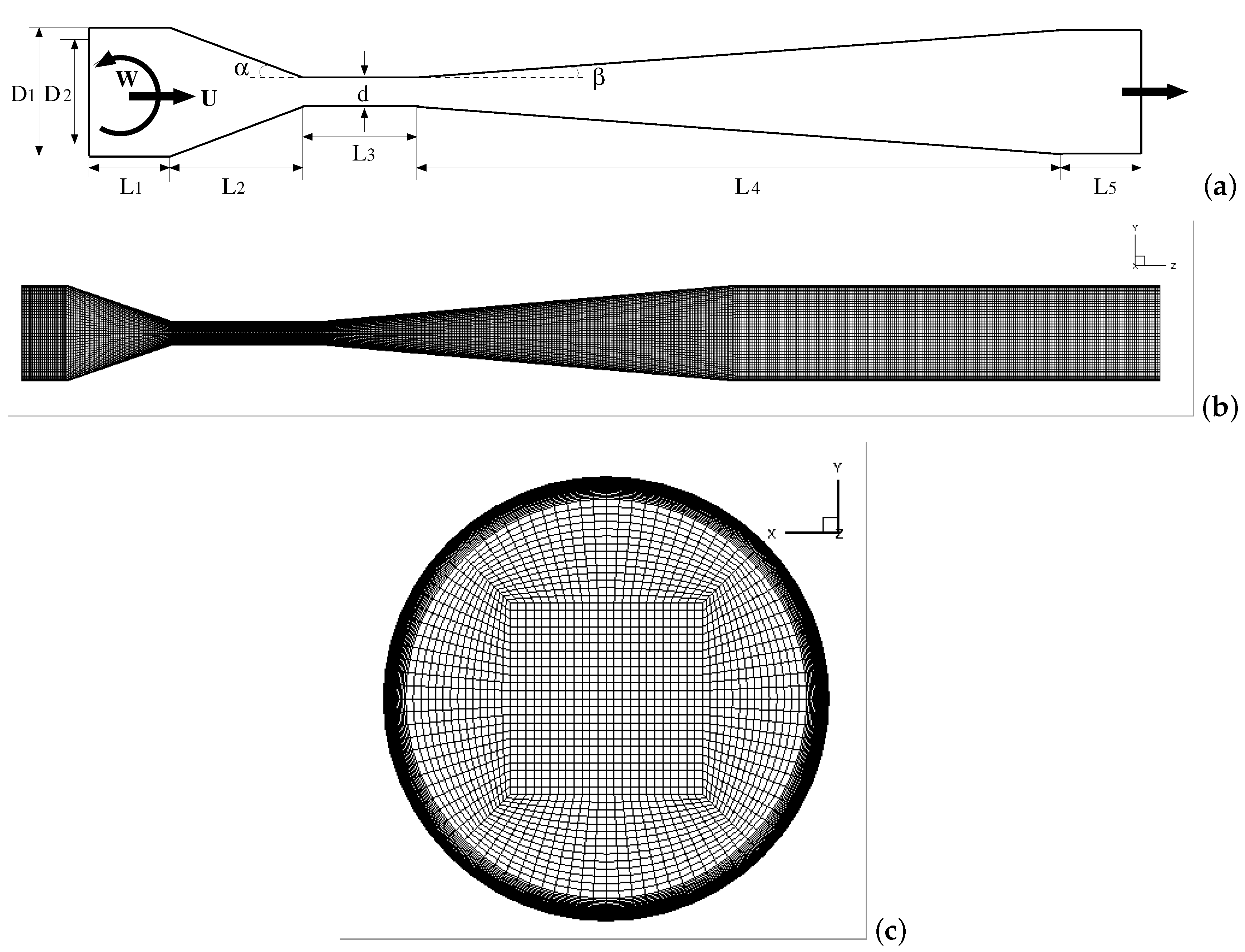
Figure 1 provides a general overview of the computational domain used in the simulations, and

Table 1. Specifications of the cavitating Venturi tube.

Parameters	Values
$D_1$ (mm)	12.7
$D_2$ (mm)	11.43
d (mm)	3.18
$L_1$ (mm)	6
$L_2$ (mm)	14
$L_3$ (mm)	20
$L_4$ (mm)	54
$L_5$ (mm)	56
$\alpha$ (${}^{\circ }$)	19
$\beta$ (${}^{\circ }$)	5

summarizes its dimensions. The swirl motion is generated at the entrance of the Venturi tube by imparting constant tangential velocity (W = 0 m/s, 0.225 m/s, 0.375 m/s, and 0.75 m/s) and axial velocity (U = 1.5 m/s) components to the flow. The corresponding Reynolds number is Re = 19,044, 19,250, 19,622, and 21,276. The mixing process between two volumetric components without chemical reactions was conducted within the liquid phase. The liquid water with a viscosity of ${\mu }_1$ = 0.001 kg/m-s (Component-1) was fed into the inner tube while the liquid water with a viscosity of ${\mu }_2$ = 0.01 kg/m-s (Component-2) flows into the outer annulus of the Venturi tube. The volume-weighted mixing law and the mass-weighted mixing law are used to calculate the mixture density ${\rho }_{m,l}$ and mixture viscosity ${\mu }_{m,l}$ of two components ($Y_1$ and $Y_2$) in the liquid phase. The physical properties for each material are specified in

Table 2. Physical properties for each material.

Material	$\mathit{\rho }$ (kg/m${}^3$)	$\mathit{\mu }$ (kg/m-s)
water−1 (Component−1)	998.16	0.001
water−2 (Component−2)	998.16	0.01
mixture (water−1−water−2)	volume-weighted-mixing−law	mass-weight-mixing−law

.

In the framework of the multiphase flow model, the homogeneous mixture model treats the mixing cavitation flows as a mixture of three fluids behaving as one. The multiphase components in the homogeneous mixture model (including three phases for vapor, Component-1, and Component-2) are assumed to share the same velocity and pressure. In the present simulation, the mixing cavitation flow is considered isothermal and incompressible, and the relative velocity between the liquid phase and vapor phase is neglected. It should be noted the assumption of vapor incompressibility may produce some deviations in vapor distribution inside a nozzle [26].

2.1. LES Model

In the present paper, the LES method is utilized to model unsteady turbulent flow in a Venturi tube. This method has been proven capable of reproducing experimental results with a high accuracy when modeling a wider range of scale of flow fields. In the spatially filtering process, the large-scale structures are directly resolved on grid scales, while the small-scale turbulence is modeled using a Subgrid-Scale (SGS) turbulence model. Because the LES method calculates directly for important large scales of motion and relies less on the modeling, the LES model is more accurate and applicable than the Reynolds-Averaged Navier–Stokes (RANS) and less computationally demanding than the Directly Numerical Simulation (DNS) method. In the present study, the Wall-Adapting Local Eddy-Viscosity (WALE) model [28] is adapted to model the subgrid-scale turbulent viscosity. The set of governing equations (mass, momentum, and component) for the 3D LES simulations are shown as follows [27]:

$$\frac{\partial }{\partial t}\left({\rho }_m\right)+\nabla ·\left({\rho }_m{\overrightarrow{u}}_m\right)=0$$

(1)

$$\frac{\partial }{\partial t}\left({\rho }_m{\overrightarrow{u}}_m\right)+\nabla ·\left({\rho }_m{\overrightarrow{u}}_m{\overrightarrow{u}}_m\right)=-\nabla P+\nabla ·\left[({\mu }_m+{\mu }_t)(\nabla {\overrightarrow{u}}_m+\nabla {\overrightarrow{u}}_m^T)\right]$$

(2)

$$\frac{\partial }{\partial t}\left({\rho }_{m,l}{Y}_i\right)+\nabla ·\left(\rho {\overrightarrow{u}}_{m,l}{Y}_i\right)=-\nabla ·(({\rho }_{m,l}{D}_m+\frac{{\mu }_t}{S{c}_t})\nabla Y_i)$$

(3)

where ${\rho }_m$, ${\overrightarrow{v}}_m$, and ${\mu }_m$ and are the density, velocity, and viscosity of the mixture phase, respectively. $S{c}_t$ is the turbulent Schmidt number with a value of 0.7, and $D_{i,m}$ is the mass diffusion coefficient for component i with a value of ${10}^{-9}$ m${}^2$/s. In addition, the mixture density ${\rho }_{m,l}$ and mixture viscosity ${\mu }_{m,l}$ of two components ($Y_1$ and $Y_2$) are calculated utilizing the volume-weighted mixing law and the mass-weighted mixing law, respectively.

The SGS eddy viscosity is determined as [27]:

$${\mu }_t=\rho L_s^2\frac{{\left(S_{ij}^d{S}_{ij}^d\right)}^{3/2}}{{\left({\overline{S}}_{ij}{\overline{S}}_{ij}\right)}^{5/2}+{\left(S_{ij}^d{S}_{ij}^d\right)}^{5/4}}$$

(4)

where ${\overline{S}}_{ij}$ is the strain rate tensor for the resolved scales, $S_{ij}^d$ is the traceless symmetric part of the velocity gradient tensor, and $L_s$ is the grid-filter width.

2.2. Cavitation Model

The Schnerr–Sauer cavitation based on the simplified Rayleigh–Plesset equation is used to calculate the mass transfer rate by solving the cavitation mass-transfer equation [27]:

$$\frac{\partial }{\partial t}\left({\alpha }_v{\rho }_v\right)+\nabla ·\left({\alpha }_v{\rho }_v{\overrightarrow{v}}_m\right)=R_e-R_c$$

(5)

where ${\alpha }_v$ is the vapor volume fraction, ${\rho }_v$ is the vapor density, and ${\rho }_l$ is the liquid density. The source terms $R_e$ and $R_c$ describe the evaporation and condensation processes of vapor bubbles in the cavitating flows, respectively, and are given as [29]:

When $P_v\ge P_l$,

$$R_e=\frac{{\rho }_v{\rho }_l}{{\rho }_m}{\alpha }_v(1-{\alpha }_v)\frac{3}{R_b}\sqrt{\frac{2}{3}\frac{P_v-P_l}{{\rho }_l}}$$

(6)

When $P_v\le P_l$,

$$R_c=\frac{{\rho }_v{\rho }_l}{{\rho }_m}{\alpha }_v(1-{\alpha }_v)\frac{3}{R_b}\sqrt{\frac{2}{3}\frac{P_l-P_v}{{\rho }_l}}$$

(7)

where $P_l$ is the fully recovered downstream pressure and $P_v$ = 2338 Pa is the saturation vapor pressure under the operating condition. The cavity radius is

$$R_b={\left(\frac{{\alpha }_v}{1-{\alpha }_v}\frac{3}{4\pi n_b}\right)}^{\frac{1}{3}}$$

(8)

where $n_b$ = ${10}^{13}$ is the bubble number density. In the present study, we assume the effect of $n_b$ on the cavitation phenomenon is limited.

2.3. Boundary Conditions and Numerics

The velocity inlet boundary condition is adapted with a constant axis velocity (U) of 1.5 m/s and a constant tangential velocity (W) of 0 m/s, 0.225 m/s, 0.375 m/s, and 0.75 m/s. The outlet is set as pressure outlet with a value of 101325 Pa. The surfaces of the computational domain are treated as non-slip walls. The boundary conditions for turbulence are specified as $5\%$ turbulence intensity and 10 for the turbulent viscosity ratio.

In the numerical calculation, the governing equations were discretized using the finite-volume method. The pressure–velocity coupling is achieved using the coupled algorithm. The momentum equations were discretized using the Bounded Central Differencing scheme. The PREssure STaggreing Option (PRESTO!) scheme [27] is selected for the pressure interpolation with the Quadratic Upwind Interpolation for Convection Kinematics (QUICK) [30] scheme used for the vapor volume fraction. The third-order Monotone Upstream-Centered Scheme for Conservation Laws (MUSCL) is used to discretize the components conservation equation. The time discretization was employed by the bounded second-order transient formulations.

The mixing flow simulations of the cavitating Venturi tube were performed with the commercial CFD software ANSYS FLUENT 16.2. The total flow time of 0.03 s was completed for each simulation. The statistics of the mean flow quantities were computed from the last 0.022 s after a stable transient solution is reached. The resolution of the computational mesh has a significant impact on the accuracy of predicted results. In order to achieve good results with a reasonable computational cost, the unsteady 3D LES cavitation simulations was conducted only with a total number of mesh elements of $3,041,280$. 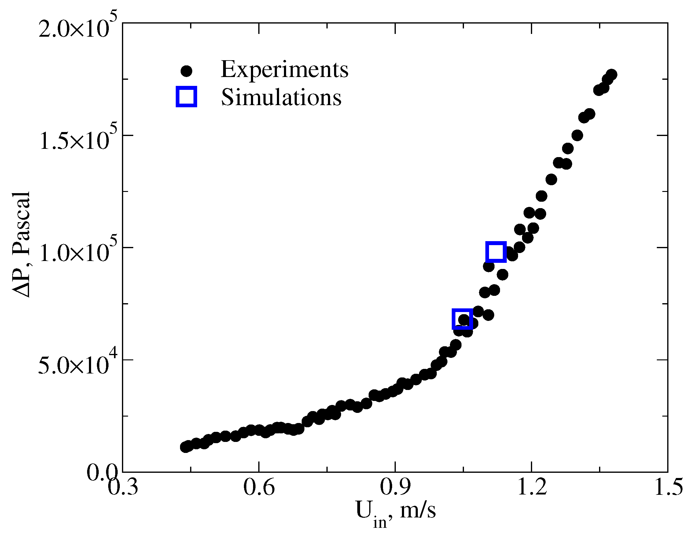This computational mesh size has been proven capable of reproducing experimental results by Shi et al. [31] in terms of statistic pressure drop under two different inflow velocities (U = 1.05 and 1.15 m/s) with a high accuracy (averaged deviation = 6.39%), as shown in Figure 4. In this work, the mesh was refined near the wall in order to achive values of $Y^{+}\approx 1.5$. The original mesh had approximately $2·{10}^6$ control volumes which results in $Y^{+}\approx 5$. However, it should be noted that the grid with $3,041,280$ control volumes is a compromise between the accuracy and time of simulations. The constant time step $\mathsf{\Delta }$t = 4 × ${10}^{-6}$ s was adapted to obtain an average Courant–Friedrich–Levy number (CFL = U$\mathsf{\Delta }$t/$\mathsf{\Delta }$x) at 0.3. The maximum number of iterations was set as 30 in the simulations. The residual value of ${10}^{-4}$ for the flow continuity was adopted as the convergence criterion.

3. Validation

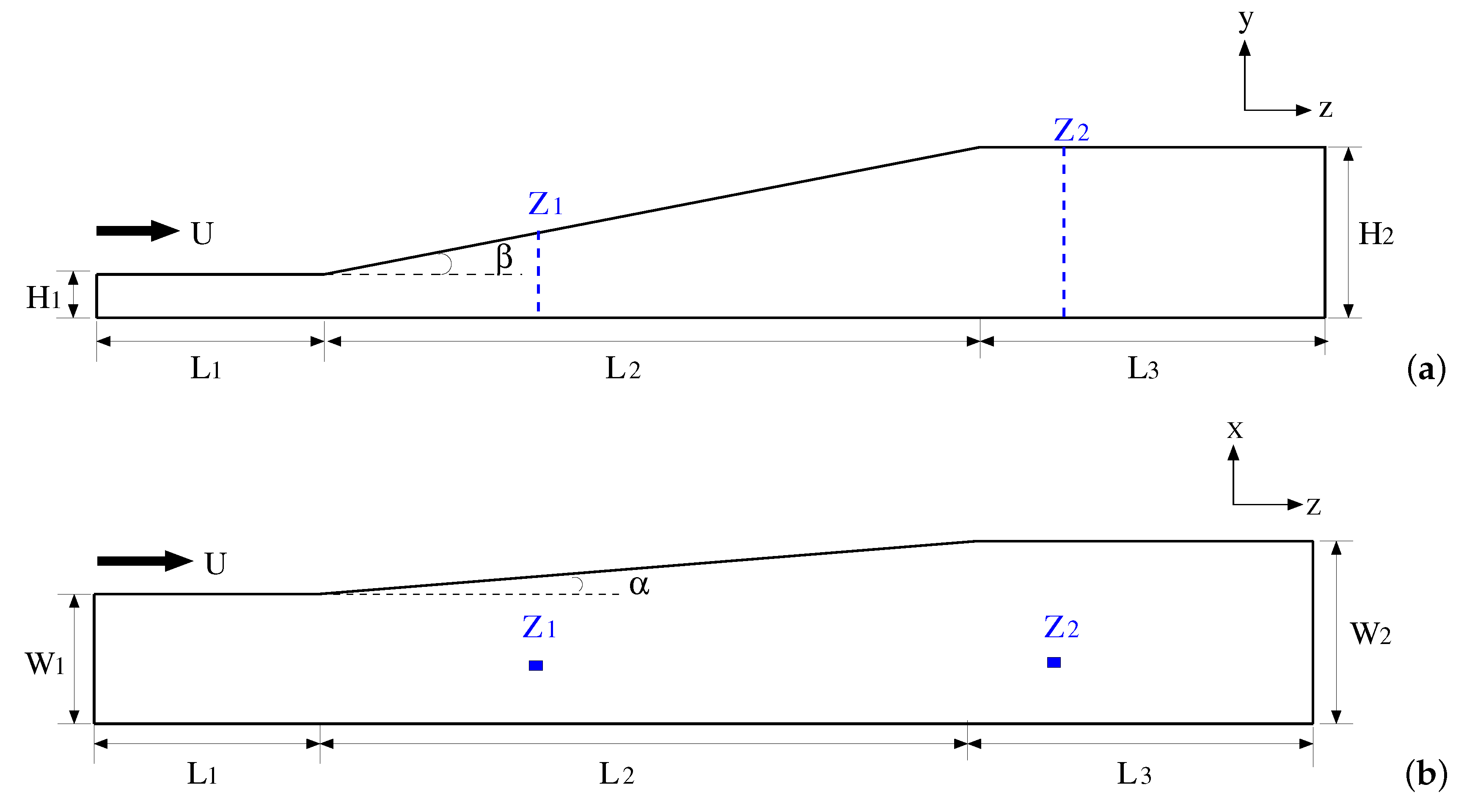
To validate the suitability of the model for the present simulation, a comparison is made between experimental results reported by Schneider et al. [32] and numerical outputs of the present study obtained within a 3D diffuser. The schema of the diffuser and its dimensions are presented in Figure 2 and

Table 3. Specifications of the diffuser. Z is measured from the start of the diffuser expansion.

Parameters	Values
$W_1$ (mm)	33.3
$W_2$ (mm)	40
$H_1$ (mm)	10
$H_2$ (mm)	40
$L_1$ (mm)	50
$L_2$ (mm)	150
$L_3$ (mm)	100
$Z_1$ (mm)	50
$Z_2$ (mm)	160
$\alpha$ (${}^{\circ }$)	2.56
$\beta$ (${}^{\circ }$)	11.3

, respectively. In the experiments, the centrifugal pump (Little Giant model No. TE-6MD-HC) is used to transport the water with a constant flow rate of 20.3 L/min. The average volume flow rate is recorded using a Signet Scientific MK315.P90 paddle wheel flow meter with an accuracy of 5% FS. The velocity data was obtained using the method of magnetic resonance velocimetry (MRV). The time-averaged streamwise velocity $U/U_b$ and vertical velocity $U_y/U_b$ are measured at two streamwise locations at the centerplane x/W${}_1$ = 0.5 (see Figure 2). 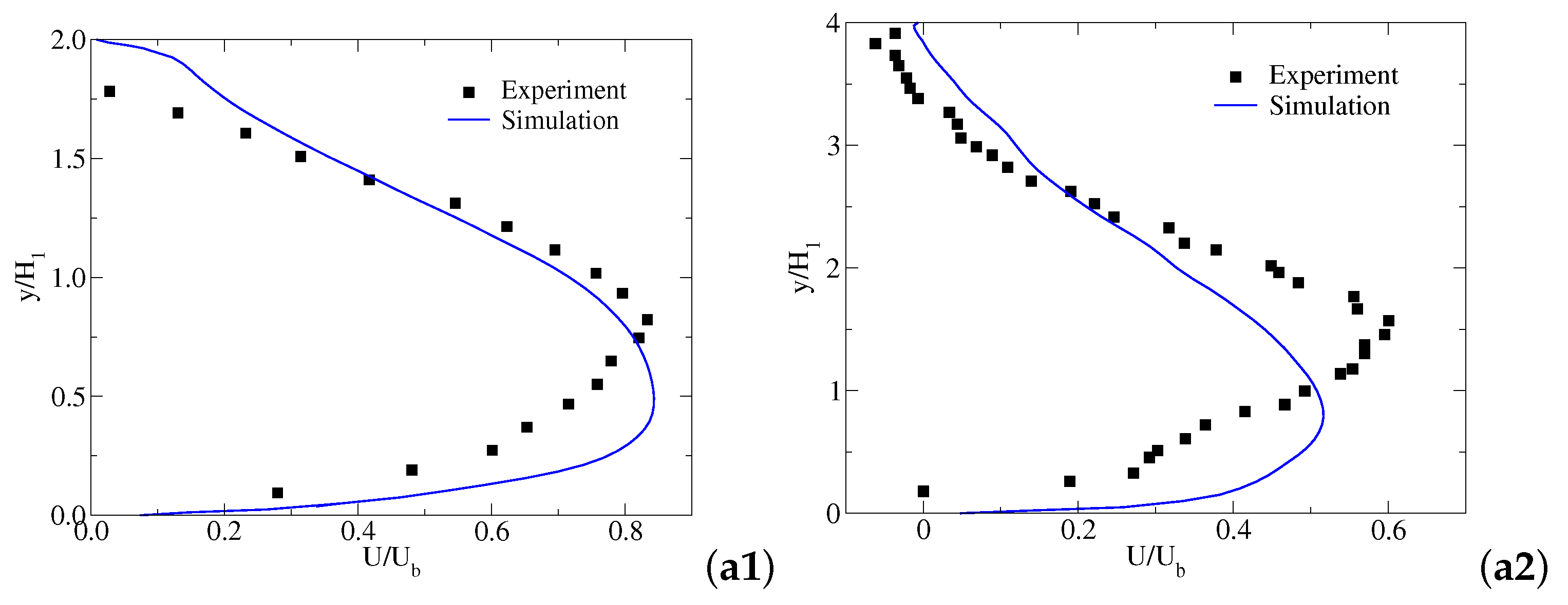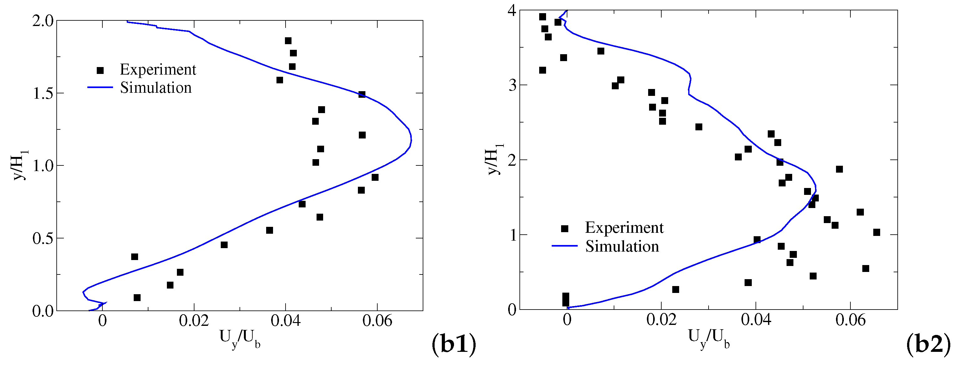Figure 3(a1,a2) show the distribution of the time-averaged streamwise velocity and vertical velocity along the centerplane at location $Z_1$ = 5$H_1$, respectively. The streamwise velocity profiles of the present study show that the LES model seems to underpredict the velocity in zones close to the lower wall. This means that more efforts should be devoted to model this region, trying to use other SGS models or refine the mesh. Even though there are some differences near the bottom of the diffuser, the overall profiles matched well with that obtained from Schneider et al. [32] experiments. Figure 3(b1,b2) exhibit the same velocity profiles at location $Z_2$ = 16$H_1$. It can be observed that the numerical models tested allow a faithful reproduction of the characteristic curves at the measured location.

A further validation using the LES turbulence model coupled with the Schnerr–Sauer cavitation model is achieved in a Venturi tube as shown in Figure 1. The experimental data are adapted from Shi et al. [6] experiments. Figure 4 presents the numerical pressure drop as a function of the inlet velocity with the experimental data as comparison. Comparison of the predicted and measured results shows a good agreement, which indicates that the present numerical models is capable of simulating the mixing flow in the cavitating Venturi tube.

4. Results

In the transient simulations, a criterion is required to evaluate the flow sate. For this purpose, we monitored the development of volume-averaged dimensionless velocity, $\frac{<U>}{U_{in}}$, with the dimensionless simulation time, $\frac{t}{t^{*}}$, under different inlet swirling ratios and found a noticeable narrow peak in the profile within $\frac{t}{t^{*}}$ = 0.08 (see Figure 5). The observed peak corresponds to the initial start-up period. After an initial start-up period, the simulations reach steady state operation. Within the steady state operation, the small velocity fluctuations can be observed from the profile. Thus, only the results of last $\frac{t}{t^{*}}$ = 0.22 were used for the analysis of the time-averaged flow field. As the swirling ratio increases from 0 to 0.5, the magnitude of the changes in the $\frac{<U>}{U_{in}}$ is significantly small. This indicates that the change in the swirl ratio from W/U = 0 to 0.5 has no large impact on the volume-averaged flow velocity.

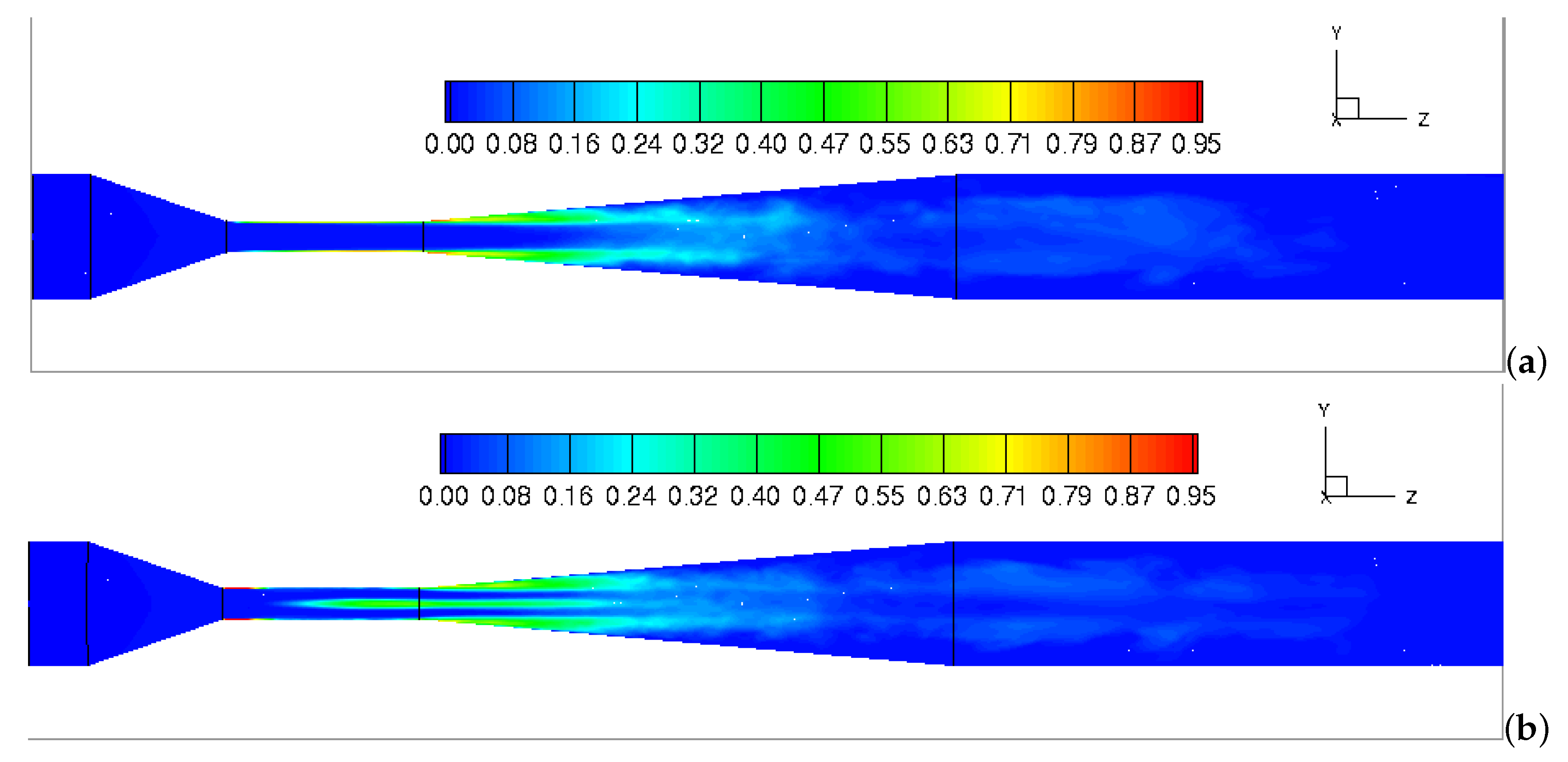
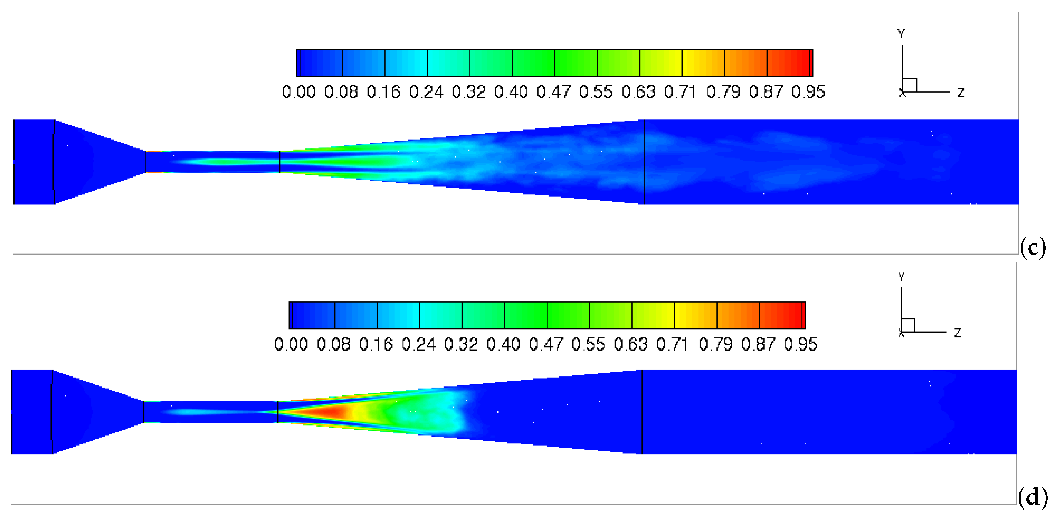
We start by analyzing the visualization of the time- and volume-averaged flow characteristics in a Venturi tube. Figure 6 presents the contour plots of time- and volume-averaged vapor volume fractions over a center plane along the domain. The cavitation patterns in the center and downstream the throat of the Venturi tube have been significantly changed by the increased swirl ratio from W/U = 0 to 0.5. With case of W/U = 0, no cavitation occurs in the full Venturi, while, when the swirl ratio increased to W/U = 0.15, a cavitation rope is formed in the central axis. The cavitation rope is a thin line structure, and the intensity of the cavitation rope reduced with its diameter decreases when the swirl ratio is further increased from W/U = 0.15 to 0.5. In addition, the conical cavitation structure can be observed in the downstream throat section at W/U = 0.5. With swirl imposed for the Venturi tube, the swirling centrifugal force is generated in the center of the Venturi tube. The low-pressure region induced by the centrifugal force is correspondingly formed along the axis. As a result, a coherent vapor core is formed in this low-pressure region with the imposition of the swirling flow.

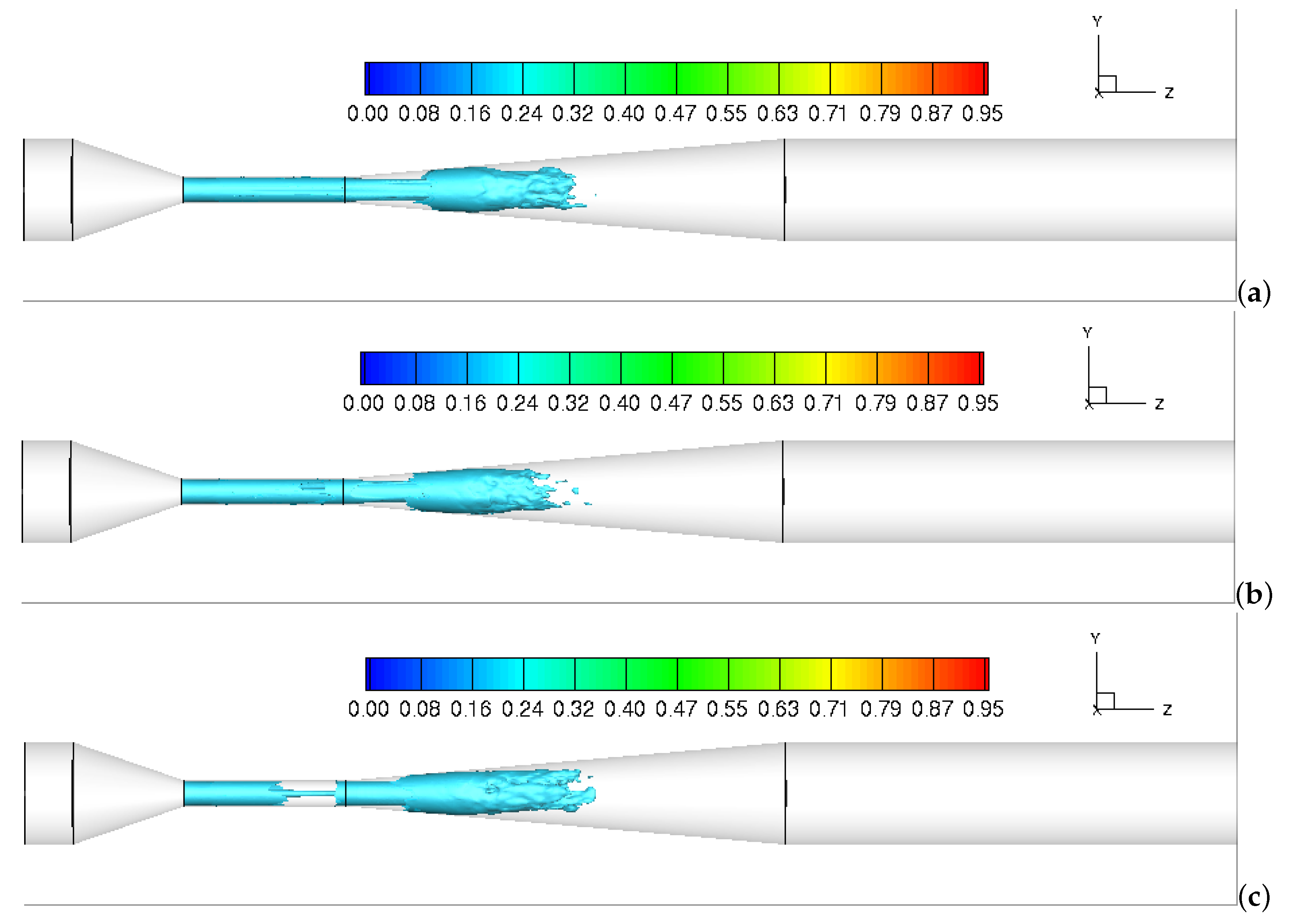
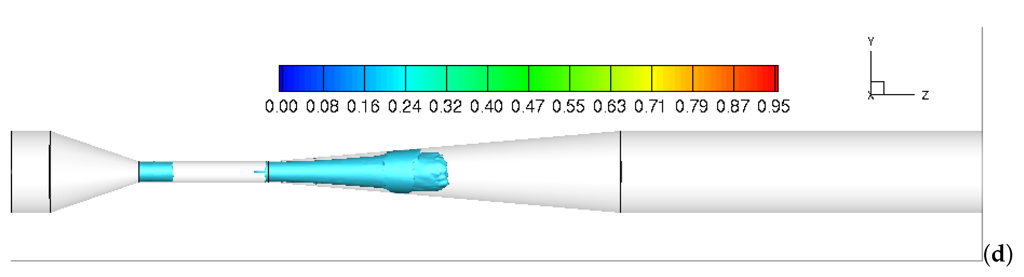
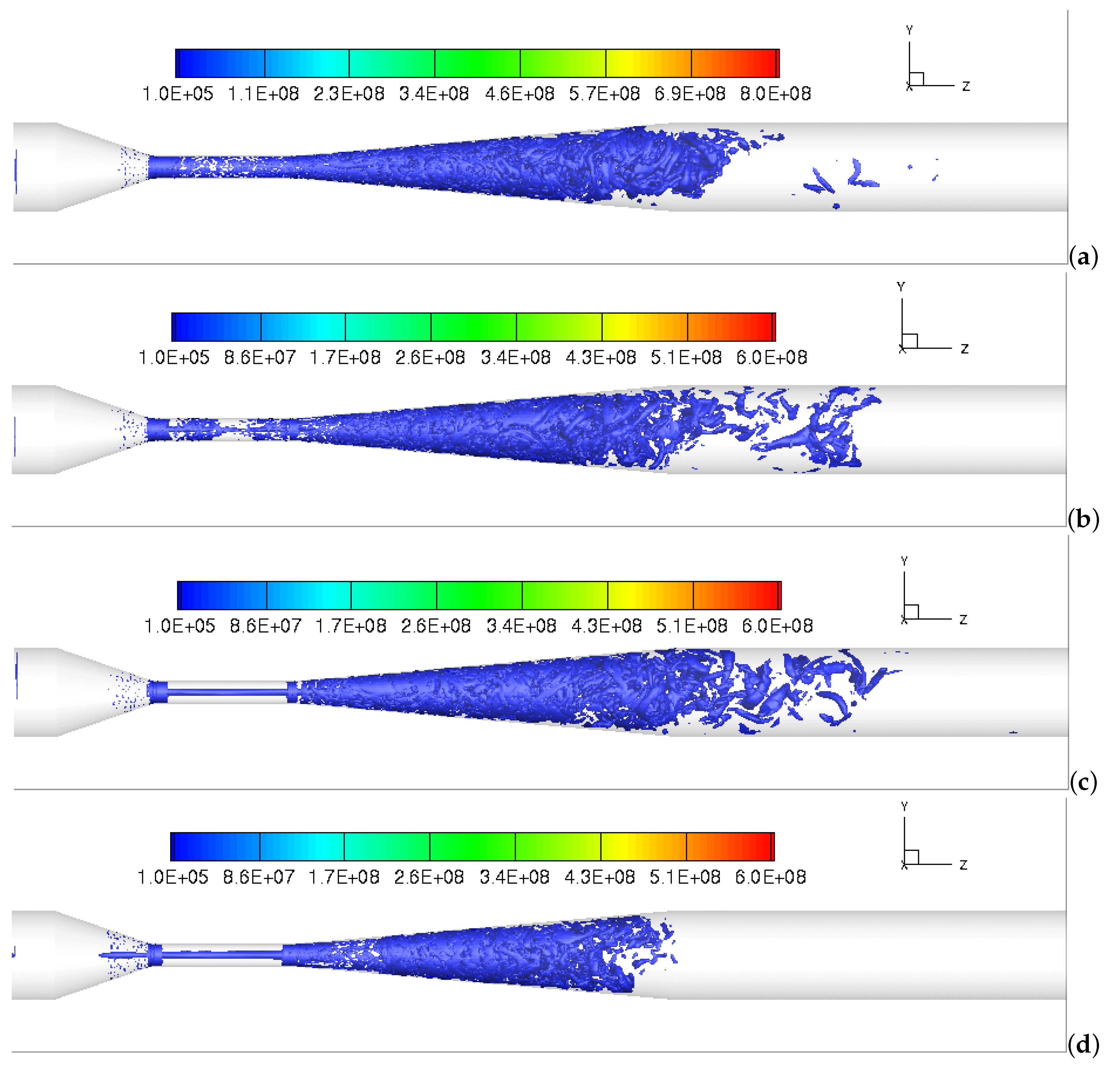
The time- and volume-averaged cavitation patterns with the iso-surface of the vapor volume fraction of 0.1 at different swirl ratios are also presented for comparison. As shown in Figure 7, the cavitation flows are initiated in the beginning of the throat section and develop along the walls into the downstream. As the swirl ratio increases from 0 to 0.5, the cavitation pattern moves inward, away from the throat surfaces toward the axis of the device. This suggests that the surfaces of throat section are far less threatened by the occurrence of the cavitation erosion with increasing device inlet swirl.

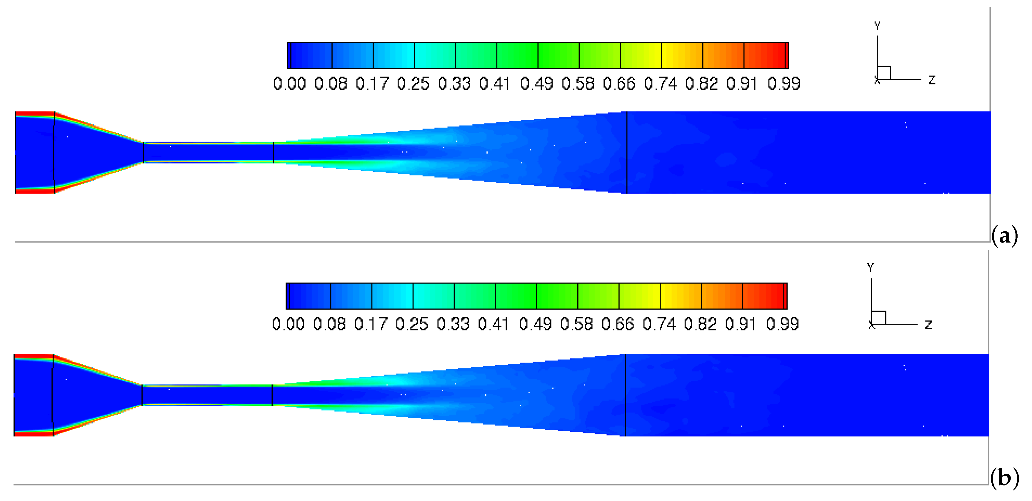
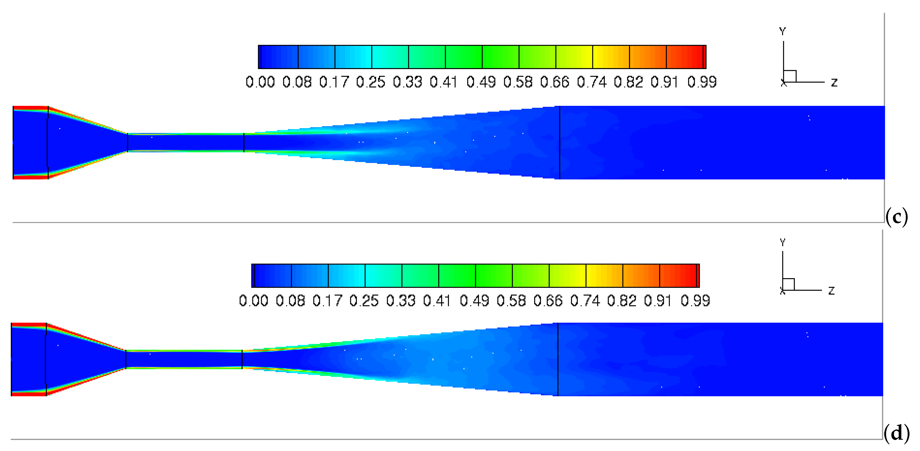
To explore the influence of inlet swirl ratios on the mixing behavior of two miscible fluids, Figure 8 shows the contour plots of the time- and volume-averaged Component-2, $Y_2$, in the center plane of the domain. As can be seen from the figures, Component-2 is fed into the outer annulus of the Venturi and penetrates the Component-1 along the Venturi walls. The mixing of two components in the downstream throat section is apparent, as is the decay of Component-2 along the axis. Small differences between $Y_2$ patterns are observed at three different inlet swirl ratios from W/U = 0 to 0.25 (Figure 8a–c). However, as the inlet swirl ratio is further increased to W/U = 0.5, an intensive mixing between two components occurs in the full divergent section (Figure 8d). The introduction of high swirl ratio produces a continuous centrifuge, and thus the intensive mixing occurs due to the high tangential velocity gradient in the downstream throat region. 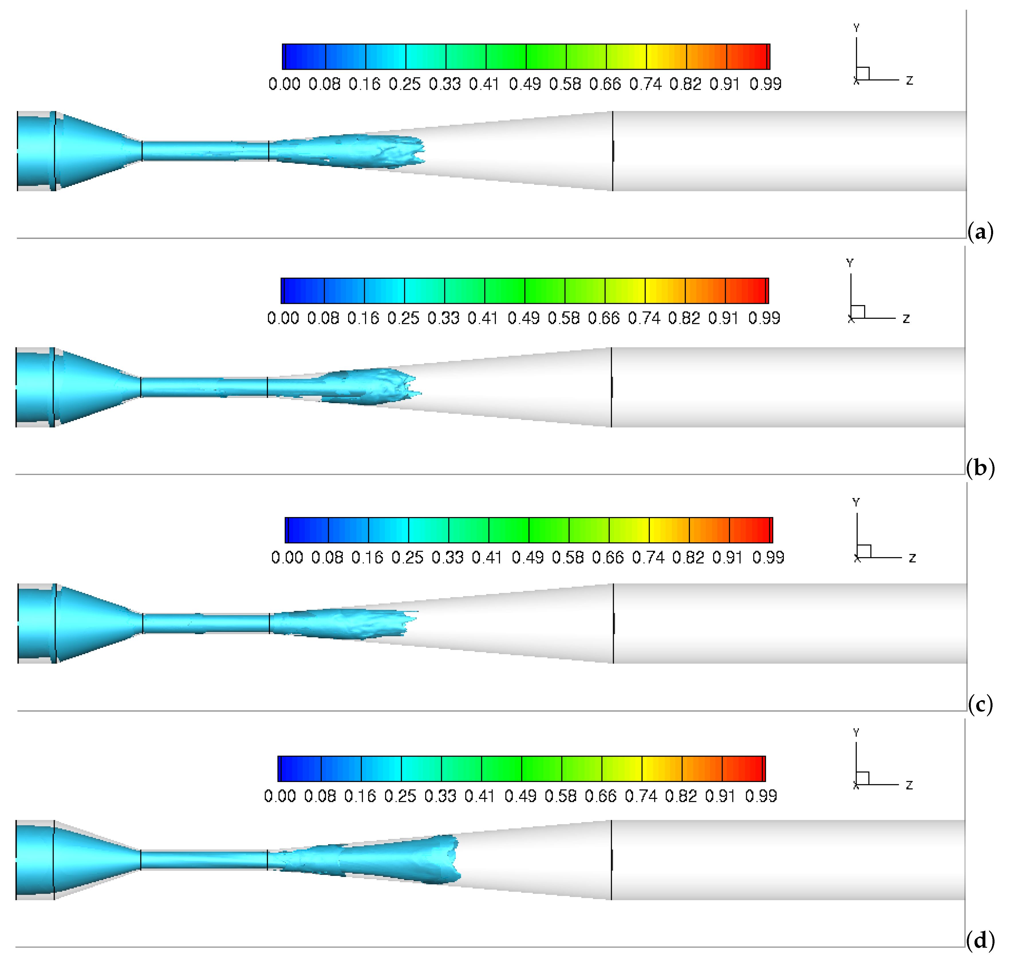Figure 9 depicts the iso-surface contours of the time- and volume-averaged Component-2, $Y_2$, under different swirl ratios. The Component regions are depicted as the iso-surfaces where the $Y_2$ reaches 0.2. As it is depicted in the figure, the components ($Y_1$/$Y_2$) mixing zone extends towards the downstream as the swirl ratio increases from 0 to 0.5. This indicates that the high concentration of $Y_2$ decreases to a low concentration as the mixing between two fluids is promoted by increasing device inlet swirl.

Figure 10 compared the results with and without swirl imposed in capturing the vortex structures. The vortex structures are more effectively shown by the visualized iso-surfaces of the Q-criterion for Q = $2\times {10}^7$ s${}^{-2}$ at $\frac{t}{t^{*}}$ = 0.3. When operating at the axial flow condition, the vortex patterns are mainly presented in the throat and divergent sections of the Venturi. With the additional swirl ratio, the thin, line vortex rope can be observed in the axis of the throat section. The vortex rope structures are basically coincide with the cavitation rope structures as shown in Figure 6. This further confirms that the vortex rope promotes the occurrence of cavitation by creating a low-pressure region in the center of the throat section.

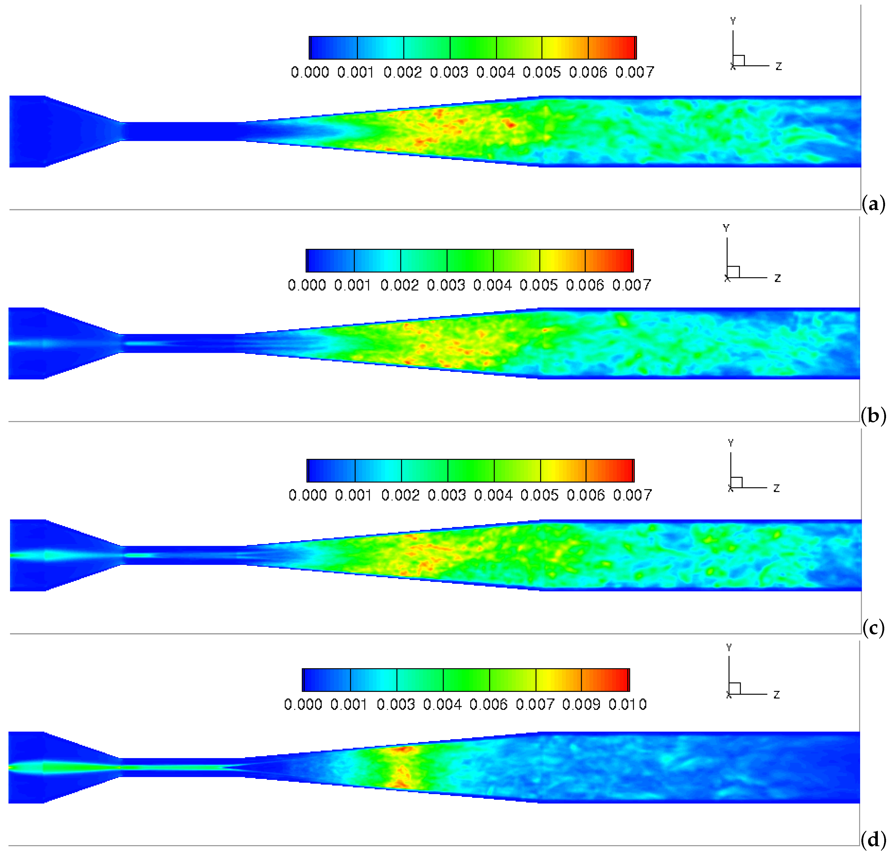
Figure 11 depicts the time- and volume-averaged subgrid turbulent viscosity ratio in the center plane of the domain. As illustrated in the figure, the higher turbulence occupies a large area in the divergent section for all simulation cases. As the imposed swirl ratio increases from 0 to 0.5, the subgrid turbulent viscosity is more extensive in the upstream core center, and the maximum value of the subgrid turbulent viscosity increases from 0.007 to 0.01. From one hand, the imposed swirling flow enhances the eddy motion and promotes rapid mixing between two fluids. From other hand, the higher turbulent viscosity causes the collapse of the bubble cluster and reduces the cavitation intensity in the downstream Venturi tube.

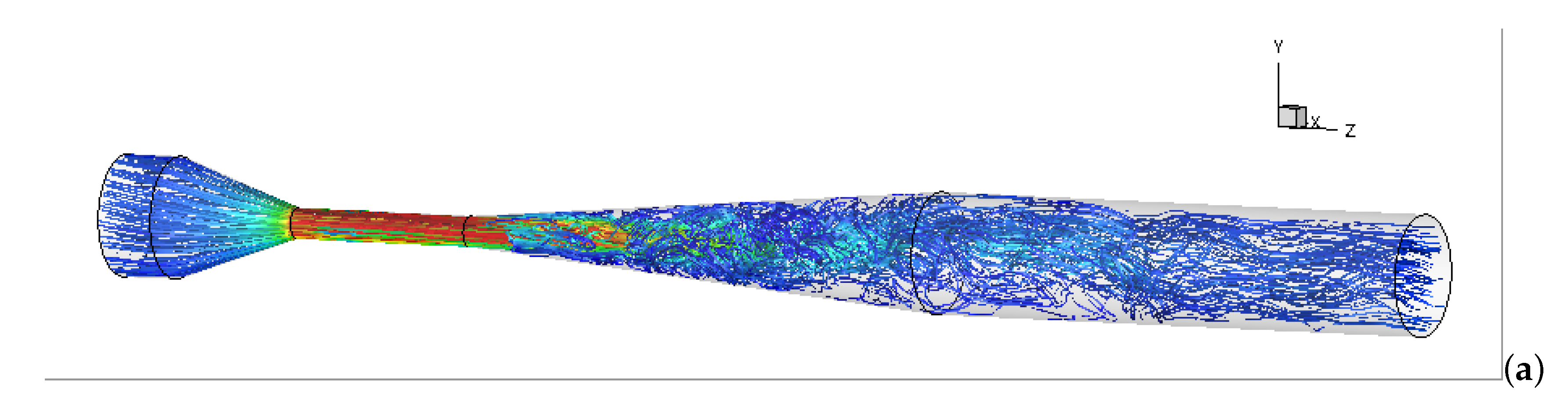
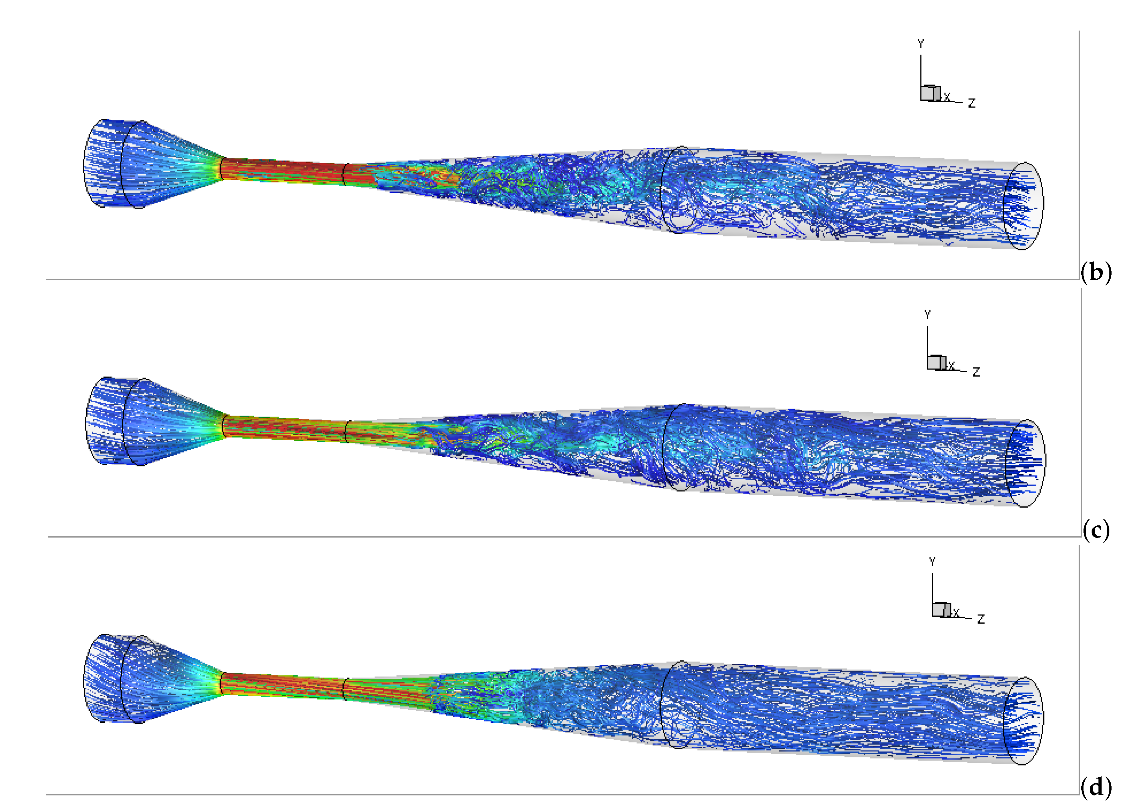
The streamlines of the mean z-axial velocities across the cavitating Venturi tube are plotted in Figure 12. When entering the Venturi tube, the magnitudes of the flow velocity are comparable for all cases. In particular, a higher velocity is present in the construction zone with a minimum cross-sectional area. From the figure, the introduction of the swirl is shown to produce an apparent radial expansion of the flow in the upstream and throat sections of the Venturi tube. The swirling flow decays along the length of the device towards the outlet.

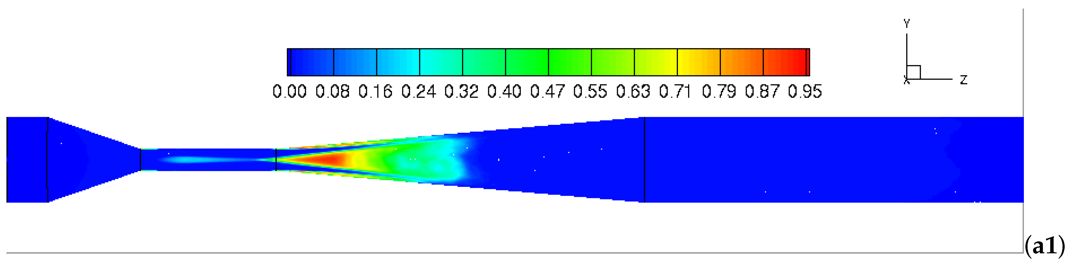
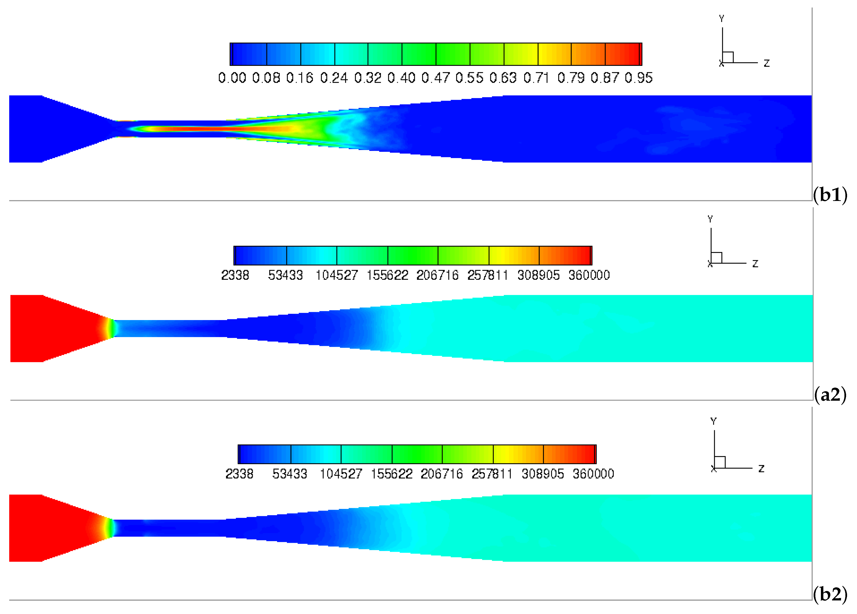
To study the effect of the fluid viscosity on the cavitating behaviors, Figure 13(a1,b1) present the time- and volume- averaged vapor volume fraction and static pressure at two different fluid viscosity ratios of $\frac{{\mu }_2}{{\mu }_1}=1$ and $\frac{{\mu }_2}{{\mu }_1}=10$. It can be observed that the intense cavitating region moves from the downstream to the center of the throat section as the fluid viscosity ratio decreases from $\frac{{\mu }_2}{{\mu }_1}=10$ to $\frac{{\mu }_2}{{\mu }_1}=1$. The results generally imply that the cavitating behaviors is largely influenced by the fluid viscosity. This phenomenon can be explained by the contours of the static pressure as shown in Figure 13(a2,b2). From the figures, we found a similar distribution of the pressure pattern for two cases. A lower pressure magnitude (2338–50,000 Pa) is present in the throat section and the beginning of the divergent section, while a higher pressure magnitude (310,000–360,000 Pa) is distributed in the upstream. As we compare the static pressure in the throat section, we found that the pressure magnitude for $\frac{{\mu }_2}{{\mu }_1}=10$ is slightly higher in the throat section than that for $\frac{{\mu }_2}{{\mu }_1}=1$. This means that the high viscous flow $\frac{{\mu }_2}{{\mu }_1}=10$ reduces the local flow velocity and consequently increases the local pressure owing to Bernoulli’s principle. As a result, the cavitating behavior is less intense for high viscous flow in the throat of the Venturi tube.

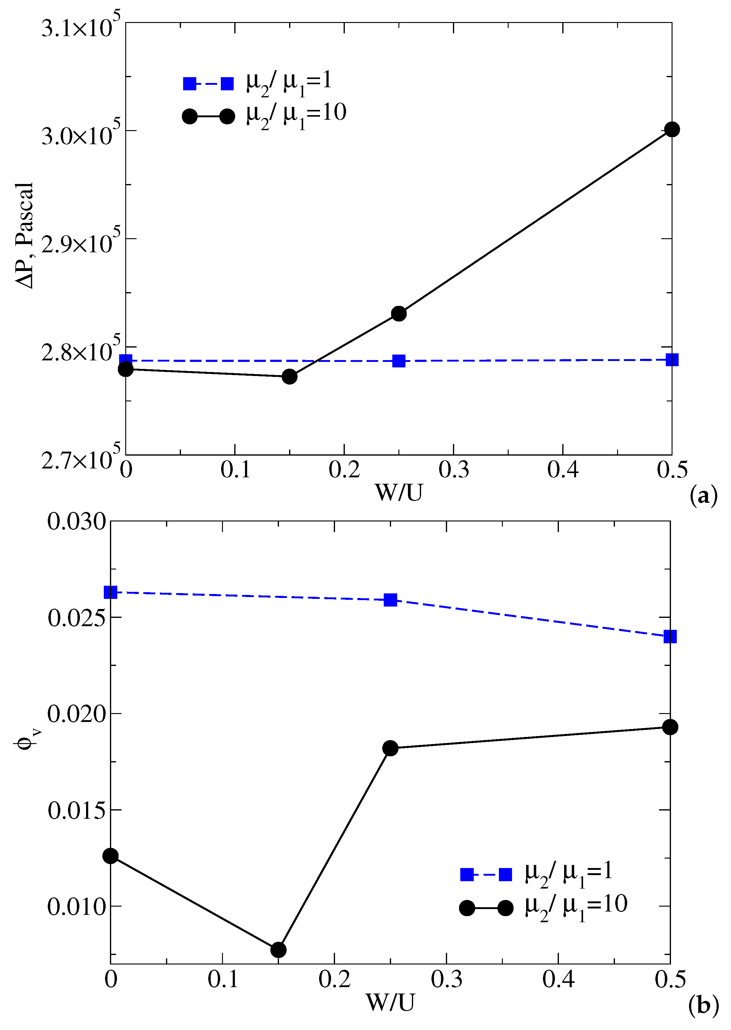
To assess the influence of the swirl ratios on the flow characteristics and the generation of cavitation, Figure 14 depicts the relationship between the static pressure drop, $\mathsf{\Delta }P$, vapor volume fraction, ${\varphi }_v$, and the swirl ratio, $W/U$. From the profiles, we noted that while a lower tangential velocity (W/U = 0.15) is imposed in the inlet, the static pressure drop remains almost constant, but the vapor volume fraction decreases significantly from 0.0126 to 0.008. As the swirl ratio further increases from W/U = 0.15 to 0.5, the static pressure drop increases linearly from 277,253 to 300,112 Pa, while the vapor volume fraction rises nonlinearly from 0.008 to 0.019. This is expected since the pressure drop required is greater when an intense swirl is introduced. Compared with the two miscible flow ($\frac{{\mu }_2}{{\mu }_1}=10$), a lower pressure drop and a higher vapor production of the pure water flow ($\frac{{\mu }_2}{{\mu }_1}=1$) can be observed as the swirl ratio increases from 0 to 0.5. The phenomenon is expected since the cavitation process only occur in pure water rather than in Component-2. In addition, the changes in the pressure drop and vapor volume fraction is significantly small of the pure water flow. This may be explained based on the fact that the high-viscosity fluids ($\frac{{\mu }_2}{{\mu }_1}=10$) results in increased resistance to the flow motion, so the pressure drop is significant. The negligible pressure drop indicates that there is almost no additional power loss and the constant pumping efficiency with the increases in swirl ratio for pure water.

5. Conclusions

In this study, a 3D CFD simulations of the mixing flows (Sc = 10${}^3$) in a cavitating Venturi tube using the commercial CFD software ANSYS FLUENT 16.2 have been conducted. An attempt is made for the first time to discuss the influence of different inlet swirling ratios (W/U = 0∼50) on the generation of cavitation and mixing behaviors in a Venturi tube. The simulation results have been validated by comparison with the experimental results from the literature. Good agreement was found between the velocity and pressure profiles obtained by the simulations and experiments. From the analysis of the results presented, we found the significant influence of imposing inlet swirl on the flow characteristics. In general, the higher the swirl ratio, the greater the vapor production, and the more efficient the mixing between two miscible fluids. As the swirl ratio increases from W/U = 0.15 to 0.5, the static pressure drop increases linearly from 277,253 to 300,112 Pa, and the vapor volume fraction rises nonlinearly from 0.008 to 0.019 in the Venturi tube. Additionally, it was shown that the cavitation bubbles move toward the axis of the Venturi away from throat surfaces when the swirl is introduced, which is favorable to minimize or eliminate the damage from cavitation erosion on the metal surfaces. Due to the enhanced eddy motion induced by the imposed intense swirl (W/U = 0.5), the mixing process between two volumetric components is promoted in the divergent section. Finally, we found that the intense cavitating region moves from the downstream to the center of the throat section as the fluid viscosity ratio decreases from $\frac{{\mu }_2}{{\mu }_1}=10$ to $\frac{{\mu }_2}{{\mu }_1}=1$. However, the changes in the pressure drop and vapor volume fraction are significantly small and of pure water flow.