Article

Interannual to Decadal Variations of Submesoscale Motions around the North Pacific Subtropical Countercurrent

1
Application Laboratory, Japan Agency for Marine-Earth Science and Technology, Yokohama, Kanagawa 236-0001, Japan
2
Department of Oceanography, University of Hawai‘i at Manoa, Honolulu, HI 96822, USA
3
California Institute of Technology, Pasadena, CA 91125, USA
4
Laboratoire d’Océanographie Physique et Spatiale, Centre National de la Recherche Scientifique, Ifremer, Plouzané 29280, France
5
Research Institute for Global Change, Japan Agency for Marine-Earth Science and Technology, Yokosuka, Kanagawa 237-0061, Japan
*
Author to whom correspondence should be addressed.
Fluids 2020, 5(3), 116; https://doi.org/10.3390/fluids5030116
Submission received: 29 April 2020 / Revised: 11 July 2020 / Accepted: 14 July 2020 / Published: 17 July 2020
(This article belongs to the Special Issue Submesoscale Processes in the Ocean)

Abstract

:
The outputs from a submesoscale permitting hindcast simulation from 1990 to 2016 are used to investigate the interannual to decadal variations of submesoscale motions. The region we focus on is the subtropical Northwestern Pacific including the subtropical countercurrent. The submesoscale kinetic energy (KE) is characterized by strong interannual and decadal variability, displaying larger magnitudes in 1996, 2003, and 2015, and smaller magnitudes in 1999, 2009, 2010, and 2016. These variations are partially explained by those of the available potential energy (APE) release at submesoscale driven by mixed layer instability in winter. Indeed, this APE release depends on the mixed layer depth and horizontal buoyancy gradient, both of them modulated with the Pacific Decadal Oscillation (PDO). As a result of the inverse KE cascade, the submesoscale KE variability possibly leads to interannual to decadal variations of the mesoscale KE (eddy KE (EKE)). These results show that submesoscale motions are a possible pathway to explain the impact associated with the PDO on the decadal EKE variability. The winter APE release estimated from the Argo float observations varies synchronously with that in the simulation on the interannual time scales, which suggests the observation capability to diagnose the submesoscale KE variability.

Graphical Abstract

1. Introduction

Submesoscale motions (involving spatial scales from 1 to several tens km) are now known to be ubiquitous in the World oceans [1]. They are enhanced in the upper oceanic layers, principally in regions with energetic mesoscale eddies (100–300 km size). A kinetic energy (KE) peak at submesoscale is observed in winter when the mixed-layer depth (MLD, H) is large enough for mixed-layer instabilities (MLI) to develop, which leads to a transformation of available potential energy (APE) into KE [2,3,4,5]. More precisely, large-scale buoyancy anomalies (forced by surface turbulent fluxes) are stirred by mesoscale eddies, which produce strong buoyancy gradients (∇b) subsequently affected by MLI. These mechanisms explain that the APE release by MLI is often parameterized as proportional to the product of the averaged horizontal buoyancy gradient (M2 =   b ¯ ) squared and the mixed layer depth squared (i.e.,   M4H2) [6,7]. Some studies emphasize that the seasonality of the APE release (due to MLI) is explained by the seasonality of both, H and M2 [1], whereas other studies point only to the role of the H seasonality [2,3,4,5]. Subsequently, the winter submesoscale KE may cascade to larger scales through an inverse KE cascade leading to the seasonality of the mesoscale KE (or eddy KE, EKE) with a time lag of two to three months [2,3,4,8,9].
The oceanic region we focus on, the subtropical Northwestern Pacific between 18° N and 28° N (Figure 1), is one of these high EKE regions. It includes the Subtropical Countercurrent (STCC) [10] (located along about 24° N from 130° E to 160° W) and the Hawaiian Lee Countercurrent (HLCC) [11] (that extends eastward from 150° E to the Hawaiian Islands along about 20° N). Using a high-resolution numerical simulation (integrated over just one year), Qiu et al. (2014) [4] found that submesoscale KE in this region exhibits a peak in late winter followed by a EKE peak in May, i.e., two months later. They also investigated the contribution of other instability mechanisms but suggested the possible role of MLI and the subsequent inverse KE cascade to explain the EKE seasonal peak.
Before Qiu et al. (2014) [4], the subtropical Northwestern Pacific ocean has drawn a lot of attention because of one of its major characteristics: the existence of significant interannual and decadal variability of its dynamics. Yoshida et al. (2011) [12] found that EKE estimated from satellite altimeter data, along the HLCC between 170° E and 160° W, varies on the decadal time scales: displaying large magnitudes in 1993–1998 and 2002–2006 and small magnitudes in 1999–2001 and 2007–2009. They further suggested that the surface heat flux changes associated with Pacific Decadal Oscillation (PDO) [13] contribute to the EKE variations. More precisely, they argued that, when the PDO is in a positive phase, the surface heat flux forcing enhances the large-scale meridional temperature gradient, elevating the EKE through the increased baroclinic instability at mesoscale. Later on, Qiu and Chen (2013) [14] tested this assumption using satellite altimeter data and temperature and salinity observations from the Argo program. They found that the EKE decadal variations between 18° N and 28° N in this region (including the STCC and HLCC) may be attributed to the instability at mesoscale of the interior zonal velocity shear induced by the surface heat flux variations. However, the observations used by Qiu and Chen (2013) [14] did not allow to investigate the impact of submesoscales.
In the present paper, we revisit the results from Yoshida et al. (2009) [12] and Qiu and Chen (2013) [14]. More precisely, following Qiu et al. (2014) [4], we raise the question of whether submesoscale motions in the upper ocean may be a pathway to explain the PDO impact on the decadal EKE variability. In other words, do the MLD and ML APE variations due to the decadal variability of surface heat fluxes (such as those associated with the PDO) lead to significant variability of the submesoscale KE that subsequently impacts EKE?
In this study, the outputs from a submesoscale permitting hindcast simulation in the North Pacific over 26 years (from 1990 to 2016) are used to examine the interannual to decadal variations of the submesoscale motions in the subtropical Northwestern Pacific including the STCC. Section 2 describes the submesoscale permitting hindcast simulation in the North Pacific. In the first subsection of Section 3, the simulated EKE variations in the STCC region are compared with those of the satellite observations. The interannual and decadal variations of the submesoscale KE enhanced in winter are next examined in Section 3.2 and Section 3.3, respectively. In Section 3.4, the contributions of these variations on the mesoscale eddies are investigated by KE cascade. In Section 3.5, we further investigate whether in-situ observations, such as the Argo float observations, are useful to diagnose the submesoscale KE variability. A summary and discussion are provided in Section 4.

2. North Pacific Submesoscale Permitting Hindcast Simulation

A submesoscale permitting hindcast simulation in the North Pacific from 1990 to 2016 was conducted to examine the interannual and decadal variations of the submesoscale motions. The model used in this study is Ocean General Circulation Model for the Earth Simulator version 2 (OFES2) [15] based on Modular Ocean Model version 3 (MOM3) [16]. The model domain covers the North Pacific from 100° E to 70° W and 20° S to 68° N at a horizontal resolution of 1/30°. The number of vertical levels is 105 with a maximum depth of 7500 m. The thickness of the first layer is 5 m, and 55 levels exist within the upper 500 m.
Numerical noises are dumped by bi-harmonic viscosities and diffusions with parameters of 1.0 × 10⁹ m4s−1 and 3.3 × 10⁸ m4s−1, respectively. For vertical mixing, diffusivities from the tidal mixing scheme [17] are added to those estimated from the mixed layer vertical mixing scheme [18] because the tidal forcing is not explicitly included in our model. Constant barotropic tidal current speeds of K1 and M2 tidal components in the existing outputs from FES2012 finite-element tide model [19] are used to estimate the energy flux at the bottom in the tidal mixing scheme. The diffusivities change in time only through the local stratification changes.
The 3-hourly atmospheric surface dataset JRA55-do ver. 1.1 [20] is used to estimate the surface fluxes. The momentum and heat fluxes are calculated with the bulk formulae proposed by Large and Yeager (2004) [21]. Note that we used the relative wind speed considering the surface current to estimate the surface momentum flux. The sea surface salinity is restored to monthly climatological values of the WOA13 v2 observations [22] with a 15-day restoring timescale to avoid unrealistic salinity fields.
This hindcast simulation was integrated from 1990 to 2016, which we call “OFES2_NP30”. The initial states are the temperature and salinity fields on 1 January 1990 from the North Pacific OFES2 simulation at a horizontal resolution of 1/10° without motions. In OFES2_NP30 the tidal motions are not explicitly included. In this study we used the daily mean outputs, in which near-inertial flows are mostly filtered out. Therefore, there are no internal tide signals and contributions of near-inertial flows are small in the outputs. We examine the submesoscale motions along the STCC considering that the circulations are mostly geostrophically balanced.

3. Results

3.1. Eddy Kinetic Energy in OFES2_NP30 and Satellite Observation

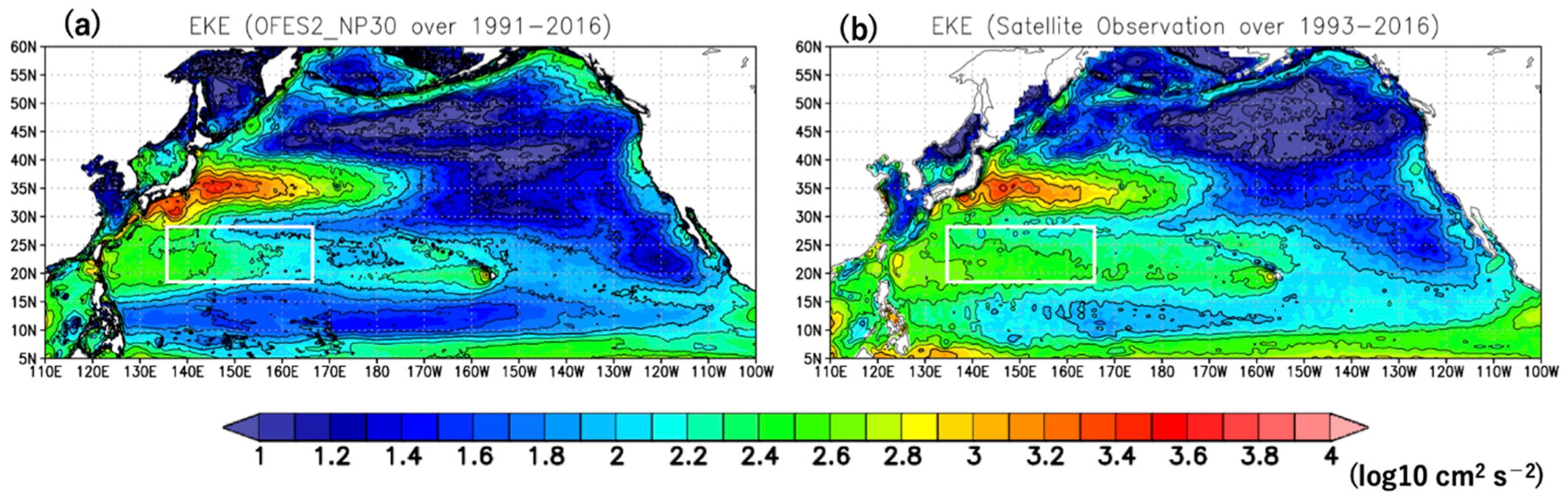
Before examining the submesoscale motions, the EKE in OFES2_NP30 is compared to the satellite observations from AVISO (https://www.aviso.altimetry.fr). The EKE is estimated geostrophically from the sea surface height (SSH) anomalies at the horizontal resolutions of 1/30° for OFES2_NP30 and 0.25° for AVISO respectively. The long-term mean EKE distributions in the North Pacific in OFES2_NP30 (Figure 1a) resemble those in the satellite observations (Figure 1b). The large EKE (>100 cm2/s2) extends from the Western Pacific to the east along the Kuroshio Extension along about 35° N, the STCC along about 22° N, and the HLCC along about 20° N to the west of the Hawaiian Islands. The high EKE along the Kuroshio Extension near Japan is slightly larger in the OFES2_NP30 than the observations. In most regions including the STCC region other than near the Kuroshio Extension, the EKE magnitudes in OFES2_NP30 are a bit smaller than the observations.
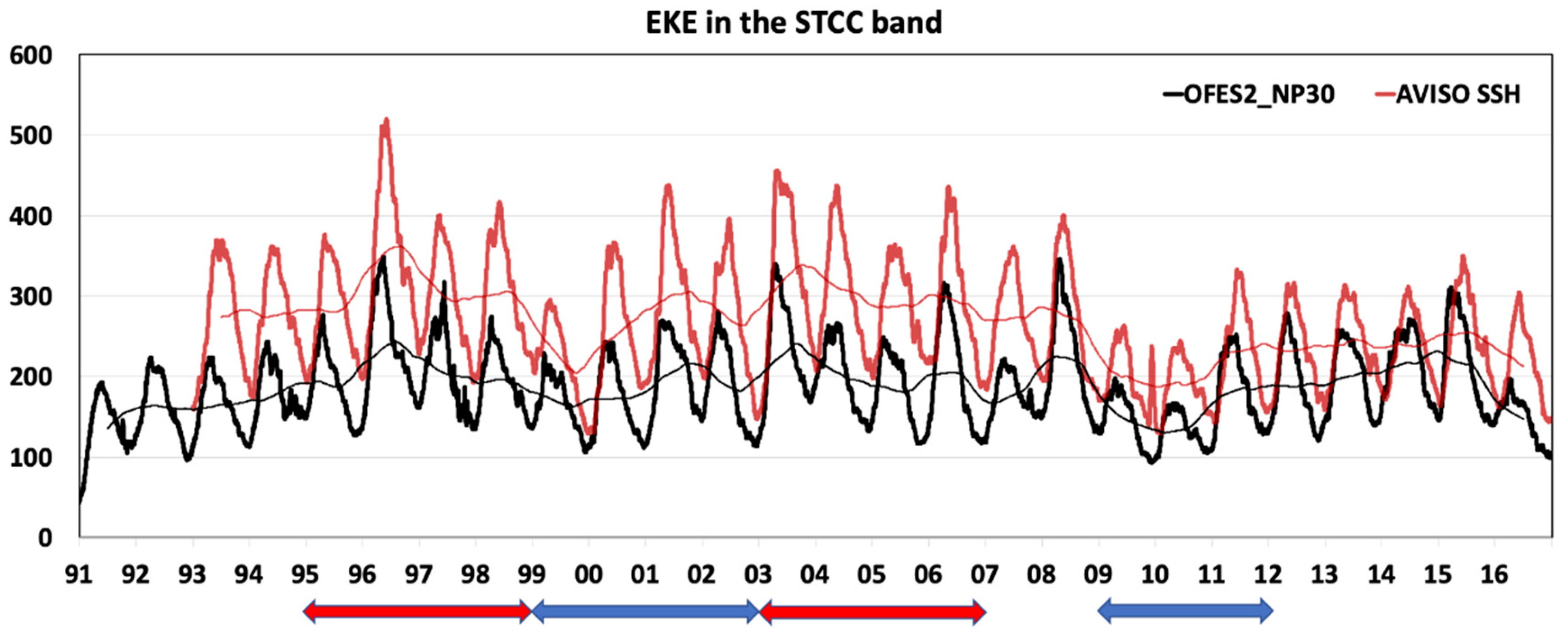
In this study, we focus on the STCC region from 135° E to 165° E between 18° N and 28° N (box region in Figure 1). The low-passed variations of the observation EKE (thin red curve in Figure 2) show high EKE in 1993–1998 with a peak in 1996 and low EKE in 1999. It gradually increased in 2000–2003 and became high in 2003–2006. In 2007–2010 it gradually decreased and became a minimum in 2010. In 2011–2016, it was relatively high. These variations are broadly similar to those shown by Qiu and Chen (2013) [14]: high in 1995–1998, and 2003–2006 and low in 1999–2002 and 2009–2011. OFES2_NP30 also captures well these decadal variations (thin black curve), although the mean EKE (187 cm2 s−2) is relatively small compared to the observations (257 cm2 s−2). This discrepancy may come from the estimation method of surface momentum flux considering the surface current in OFES2_NP30 as previous studies suggest [23,24]. In addition to the decadal variations, the EKE was anomalously high in 1996 and low in 1999, 2009, and 2010 in both OFES2_NP30 (thick black curve) and the observations (thick red curve), revealing the EKE interannual variations in the STCC region. Note that the EKE in OFES2_NP30 peaks earlier by about 1.5 months than the observations. This time lag is probably attributed to the different resolutions between the datasets as shown by Qiu et al. (2014) [4]. OFES2_NP30 at a horizontal resolution of 1/30° simulates well the submesoscale motions whose KE peaks in late winter. On the other hand, the satellite observations at a horizontal resolution of 0.25° capture the motions at scales larger than mesoscale, whose EKE peaks in spring to early summer. These results show that OFES2_NP30 represents well the interannual to decadal EKE variations in the STCC region, although a few discrepancies exist as shown above. In the later subsections, the interannual to decadal variations of the submesoscale motions in the STCC region are examined by using the outputs from OFES2_NP30.

3.2. Interannual Variations of Submesoscale Motions in the STCC Region

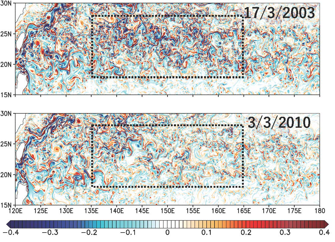
The daily mean surface relative vorticity on a winter day in 1996 (Figure 3a) in OFES2_NP30 shows that submesoscale motions of small eddies and elongated filamentary features are ubiquitous in the Northwestern Pacific regions around the STCC. These small features are prominent along the southern (21° N) and northern (25° N) STCCs. We examine interannual to decadal variability of the active submesoscale motions in winter accompanied by the STCC.
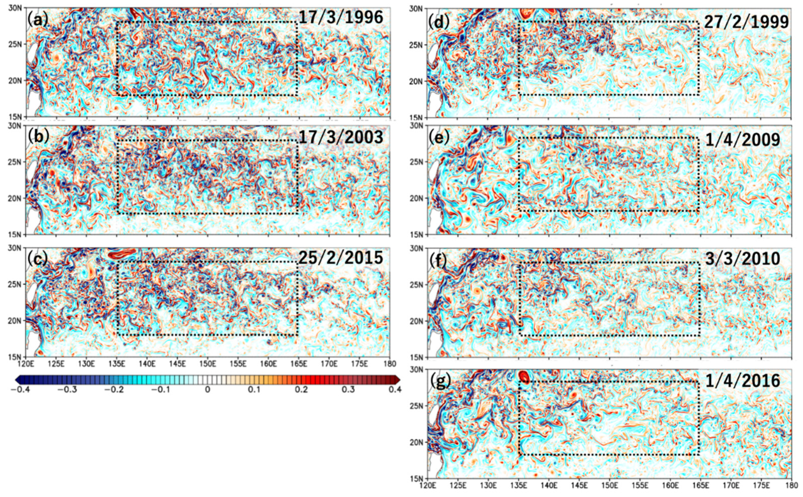
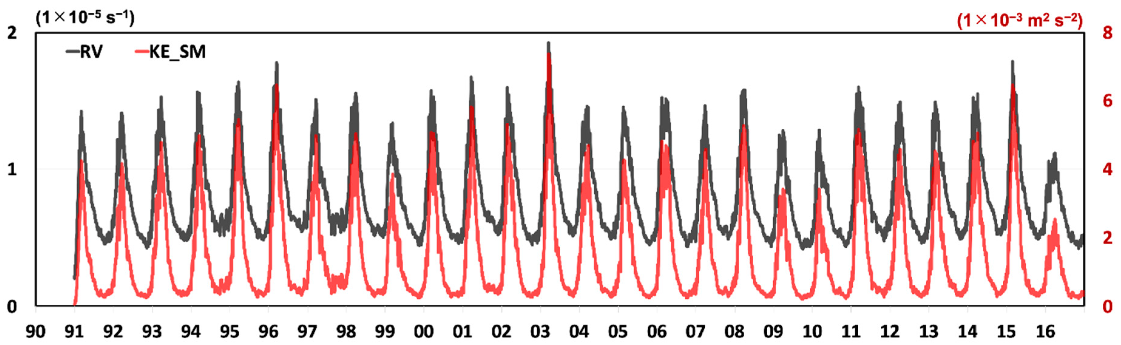
Figure 4 shows daily mean time series of the root mean square (RMS) surface relative vorticity averaged in the STCC region (black curve). The RMS vorticity varies seasonally: large in winter (February and March), which is consistent with the seasonality of the submesoscale EKE in the STCC region revealed by Qiu et al. (2014) [4]. In addition, the RMS vorticity peak in winter varied interannually: anomalously large in 1996, 2003, and 2015 and small in 1999, 2009, 2010, and 2016. The distributions of surface relative vorticity in the day with the maximum RMS vorticity in each year also display these interannual variations: ubiquitous/active and calm submesoscale motions in these years, respectively (cf. left versus right panels in Figure 3).
In this study, the surface submesoscale KE with wavelengths shorter than 100 km (KE_SM) averaged in the STCC region is examined to diagnose the variability of submesoscale motions. The time series of daily mean submesoscale KE (red curve in Figure 4) displays the distinct seasonality, which is more apparent than the RMS relative vorticity (black curve). The submesoscale KE (red curve) is very small from late summer to autumn (~3 × 10⁻⁴ m2 s−2), increases rapidly in winter and peaks in late winter (>2 × 10⁻³ m2 s−2).
The winter submesoscale KE also varied on the interannual time scales (KE_SM, red curve), similar to the RMS relative vorticity (black curve): large in 1996, 2003, and 2015 and small in 1999, 2009, 2010, and 2016. To reveal how the winter submesoscale KE vary interannually, the process of MLI enhancing the submesoscale KE is considered. The baroclinic instabilities develop at the submesoscale within the mixed layer, which enhances the submesoscale KE and leads to the restratification within the upper ocean. Fox-Kemper et al. (2008) [7] parameterized the MLI considering an overturning streamfunction whose isopycnal surface tilts from the vertical to the horizontal. They proposed that the available potential energy (APE) release in the process of MLI is proportional to the product of the front-averaged horizontal buoyancy gradient (M2) squared, the mixed layer depth (MLD, H) squared, and the inertial period (1/f, f is the Coriolis parameter),
ΔAPE/Δt ∝−(C−1) M4 H2/C |f|,
where C is a ratio of eddy flux slope to isopycnal slope (see detail in Fox-Kemper et al. 2008 [7]).
In this study, the value of C is 2: a typical value suggested by a previous study [7]. The surface meridional buoyancy gradient (My2) is used instead of M2 because the horizontal buoyancy gradient is mostly in the meridional direction in the STCC region (not shown) and buoyancy does not change much within the mixed layer. Thus, the APE release (−ΔAPE/Δt) becomes
−ΔAPE/Δt ∝ 0.5 My4 H2/|f|.
We will examine the right-hand side (=0.5 My4H2/|f|) as the APE release.
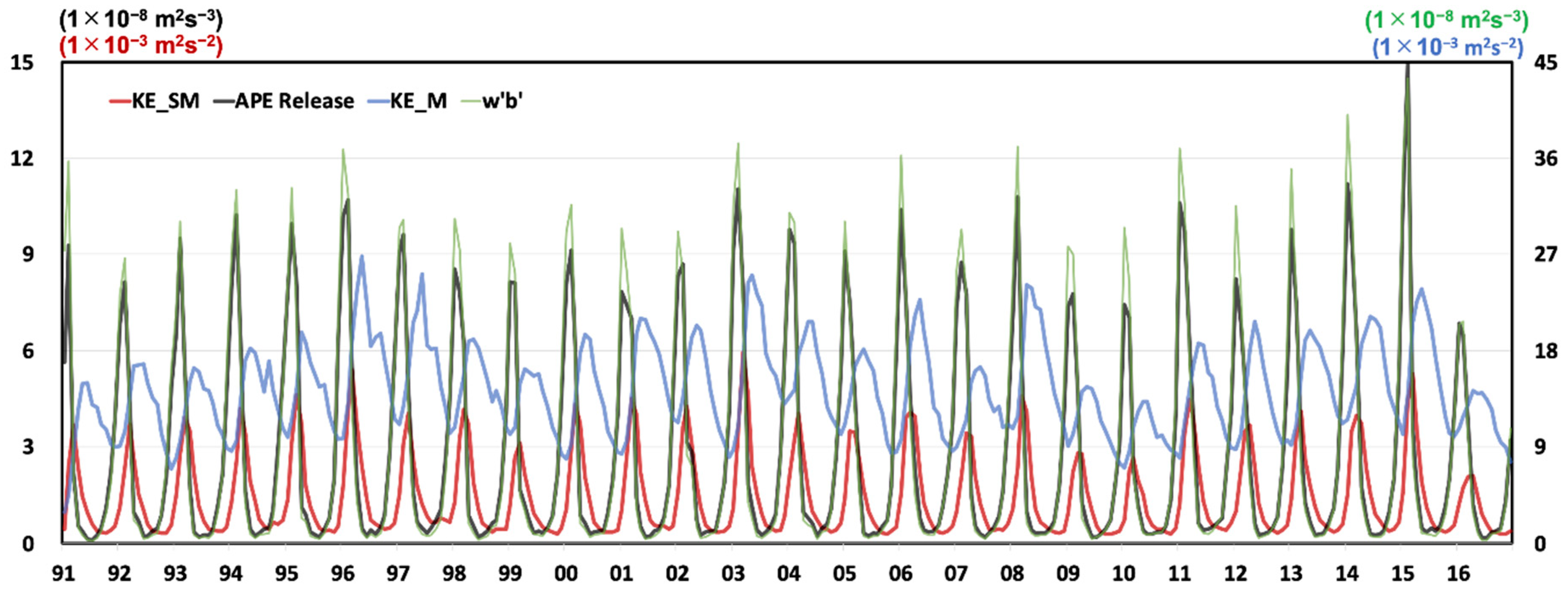
The monthly time series of the parameterized APE release in the STCC region (black curve in Figure 5) synchronously varies with the APE release directly estimated from OFES2_NP30 outputs (w’b’, green curve in Figure 5, where w and b are vertical motion and buoyancy and the prime denotes the deviation from the local area mean of 10° × 10° subdomain). This synchronization suggests that the estimation of the parameterized APE release (Equation (2)) is qualitatively reasonable. Its magnitude however is about one third of the direct estimation, which suggests that it partially explains the amount of APE release. One possible reason of its small magnitude is the buoyancy gradient only in the meridional direction. Moreover, the mechanisms inducing the submesoscale motions other than MLI should be the candidates (see detail in Section 4). In the present study, the parameterized APE release (Equation (2)) is used based on the synchronization with the direct estimation.
The APE release varies seasonally (black curve in 
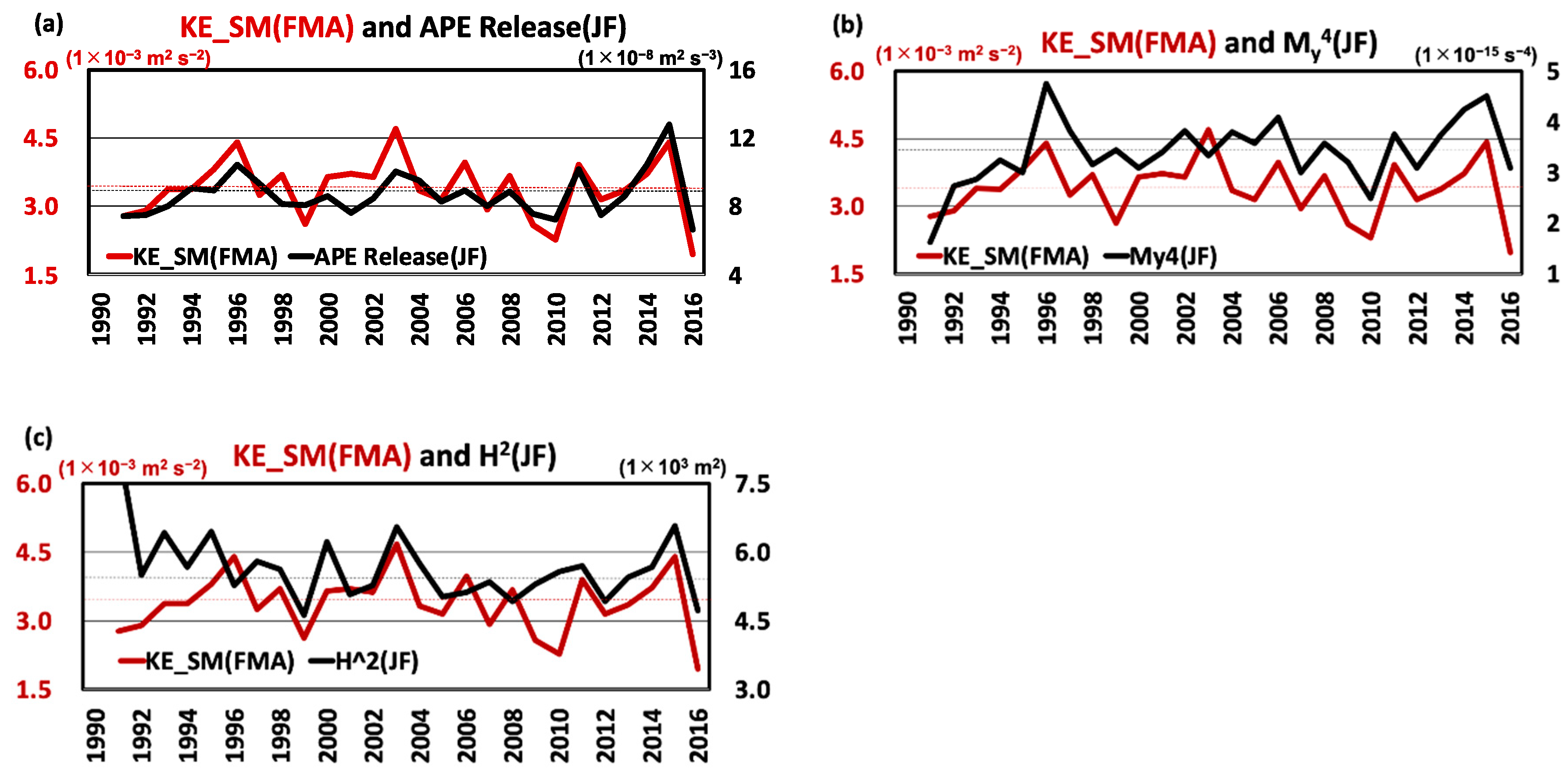
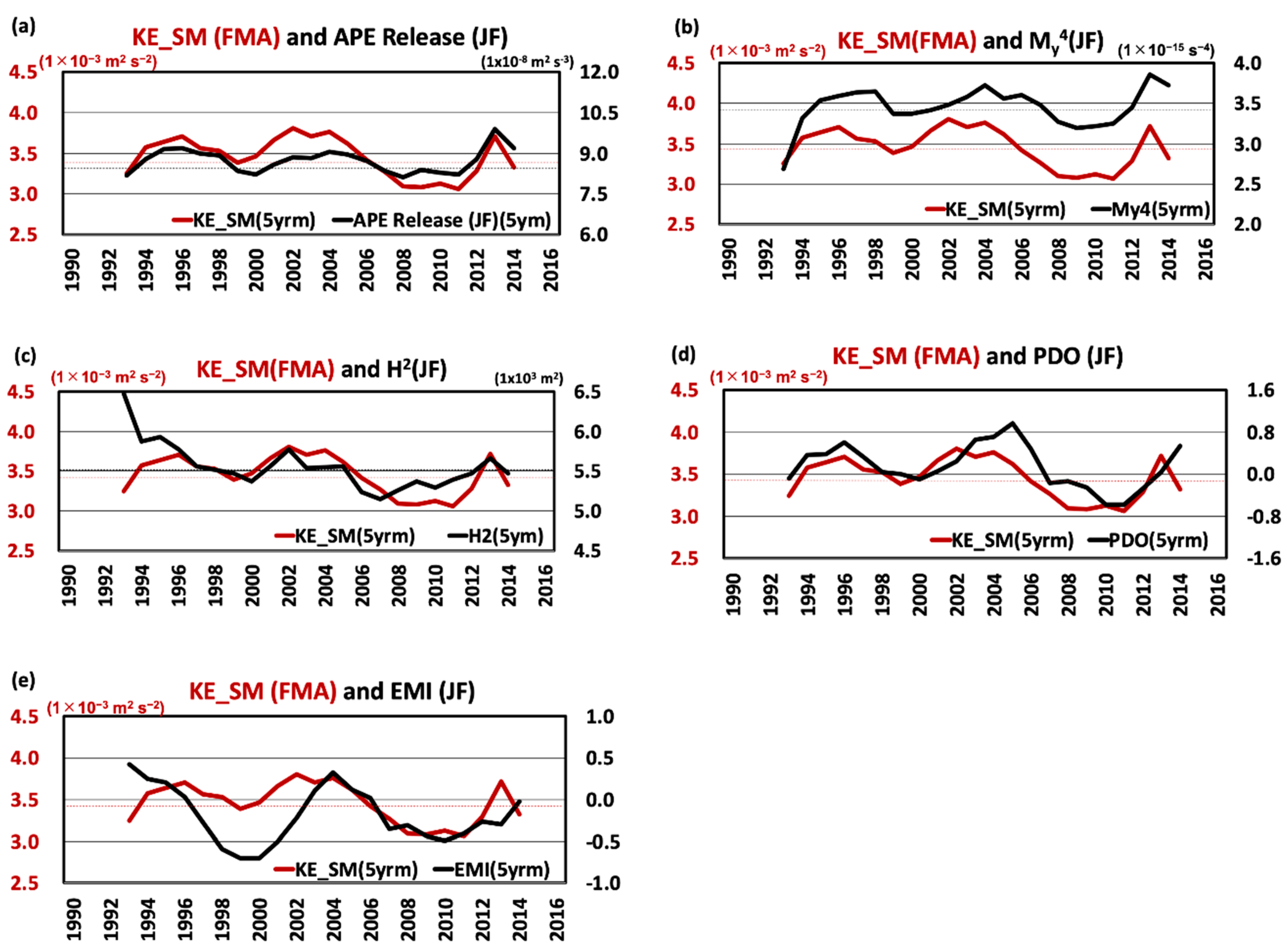
Figure 5): peaks in winter and bottoms in late summer and autumn. The peaks and bottoms of submesoscale KE (red curve) follow those of the APE release with one or two months lag. This time lag can be explained by energy budget of submesoscale motions: the submesoscale KE increases via the APE release and decreases via KE cascades to the other scales. In addition to the seasonality, the peaks of the submesoscale KE and APE release in winter appear to vary synchronously on the interannual time scales. To show these interannual variations more clearly, the annual time series of the submesoscale KE averaged from February to April (red curve) and the APE release averaged from January to February (black curve) were made (Figure 6a). Both time series vary synchronously and the correlation between them is high (0.77). These results suggest that the interannual variations of the APE release in the process of the MLI lead to the submesoscale KE variations in the STCC region.
The APE release depends on the APE within MLD: proportional to the squares of the horizontal buoyancy gradient (My2) and MLD (H) (see Equation (2)). How much does each component contribute to the variations of submesoscale motions? The interannual variations of either My4 (black curve in Figure 6b) or H2 (black curve in Figure 6c) vary less synchronously with the submesoscale KE variations (red curves in Figure 6) than the APE release (black curve in Figure 6a). The correlations between the variations of either My4 or H2 and submesoscale KE are 0.59 and 0.52, respectively, which are smaller than 0.77 between submesoscale KE and APE release. Table 1 shows that the submesoscale KE was large (small) in the years when the APE release was high (low). However, these anomalous submesoscale KE events were not always induced either by anomalous horizontal buoyancy gradient (My4) or MLD (H2). The submesoscale KE in the STCC region is modulated on the interannual time scale by the APE release, but less influenced by either of the horizontal buoyancy gradient or the MLD.

3.3. Decadal Variations of Submesoscale Motions in the STCC Region

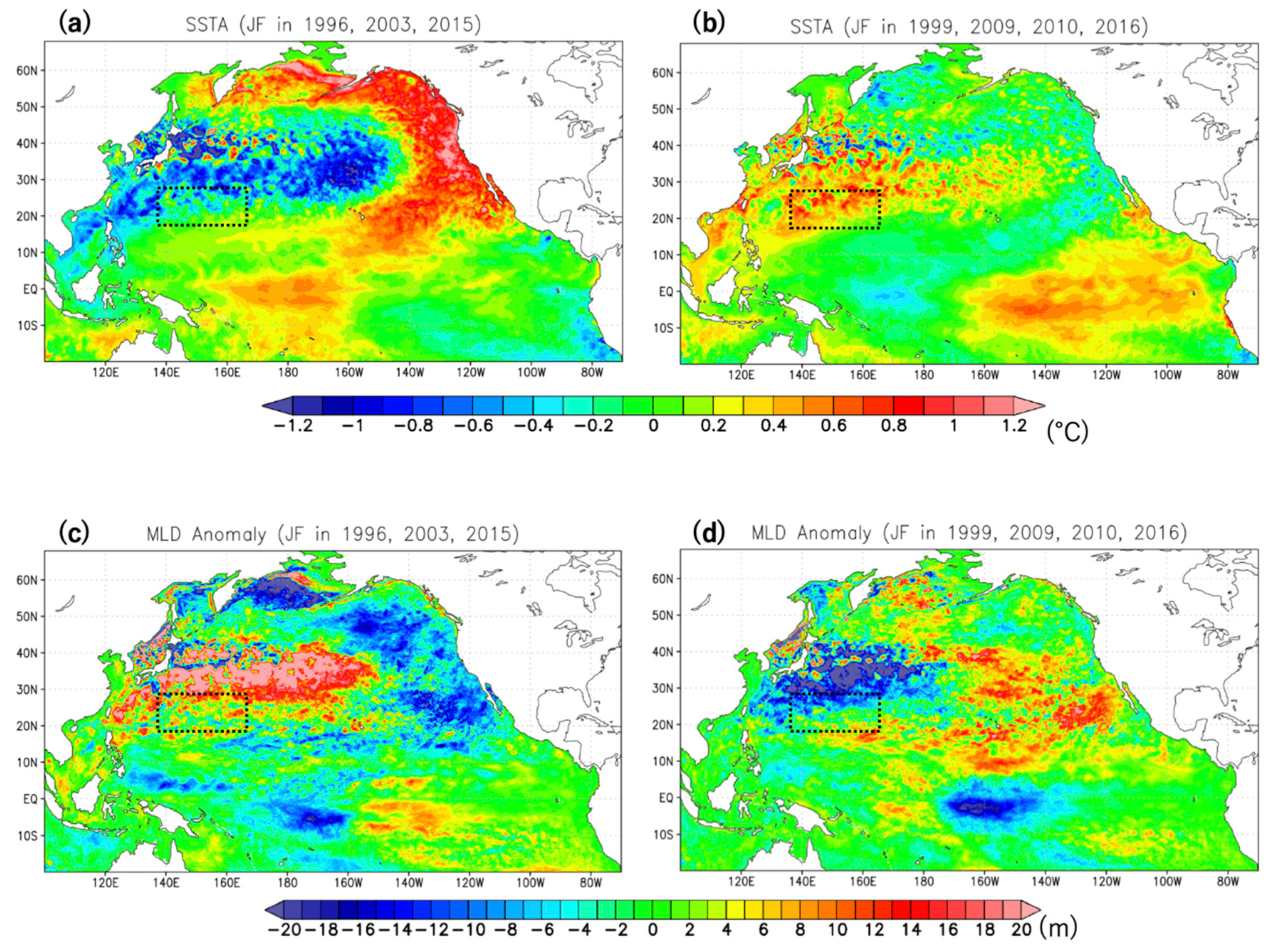
Figure 7 shows the composite distributions of sea surface temperature (SST) anomaly and MLD anomaly averaged from January to February in the years with the large and small winter submesoscale KE in the STCC region. The SST anomaly with the large submesoscale KE is characterized by the horseshoe shape of warm SST in the Eastern Pacific surrounding cool SST in the mid and western Pacific between 20° N and 50° N (Figure 7a). This pattern resembles the positive phase of the PDO. In contrast, the SST anomaly pattern in Figure 7b with the small submesoscale KE is similar to that in the negative phase of the PDO. These results suggest that the decadal variations of submesoscale motions in the STCC region is associated with the PDO.
To clarify this relation, the lowpass filtered variations of the submesoscale KE, parameterized APE release in the STCC region, and the PDO index in winter are plotted (Figure 8a,d). The submesoscale KE (red curves) synchronously varies on the decadal time scale with the PDO index (black curve Figure 8d), and also with the APE release (black curve Figure 8a). Both the submesoscale KE and APE release were large when the PDO index was positive in 1995–1997 and 2001–2005. Whereas they were small during the negative PDO index in 1999–2000 and 2009–2011. These results suggest that the submesoscale KE is modulated on the decadal time scale by APE release variations associated with the PDO. Note that the decadal variations of submesoscale KE are similar to the EKE variations (Figure 2).
In the STCC region when the submesoscale KE is large, the anomalous cool SST to the north (Figure 7a) possibly enhances the surface meridional buoyancy gradients considering the thermal expansion. Additionally, the MLD (Figure 7c) is deep by about 3.6 m averaged in the STCC region. These enhanced buoyancy gradients and the deepened MLD can increase the APE release based on Equation (2). Conversely when the submesoscale KE is small, the anomalous warm SST to the north (Figure 7b) and the shallow MLD (about 2.9 m) (Figure 7d) in the STCC region tend to decrease the APE release. These results suggest that both the buoyancy gradient and MLD variations, associated with the PDO contribute on the APE release change on the decadal time scale. However, either buoyancy gradient squared (My4, black curve in Figure 8b) or MDL squared (H2, black curve in Figure 8c) vary a little less synchronously with the submesoscale KE (KE_SM, red curves) than the APE release (black curve in Figure 8a). Similar to the interannual variations in the previous subsection, these results suggest that the decadal variations of the submesoscale motions are modulated by the APE release depending on the buoyancy gradient and MLD, but not solely by either one.

3.4. KE Cascade in the STCC Region

To examine how the interannual variations of submesoscale motions influence the other scales, we examine the variations of the KE cascade process. The surface spectral KE flux is estimated by
Π ( k ) =   k k s R e ( u * ^ · ( u · H u ^ ) ) ( k ) d k ,
where u is the velocity vector at the surface, carets are discrete Fourier transform, ∇H is the horizontal gradient operator, and asterisks are complex conjugates. k is the wavenumber and ks is the largest one corresponding to the horizontal resolution of OFES2_NP30. 
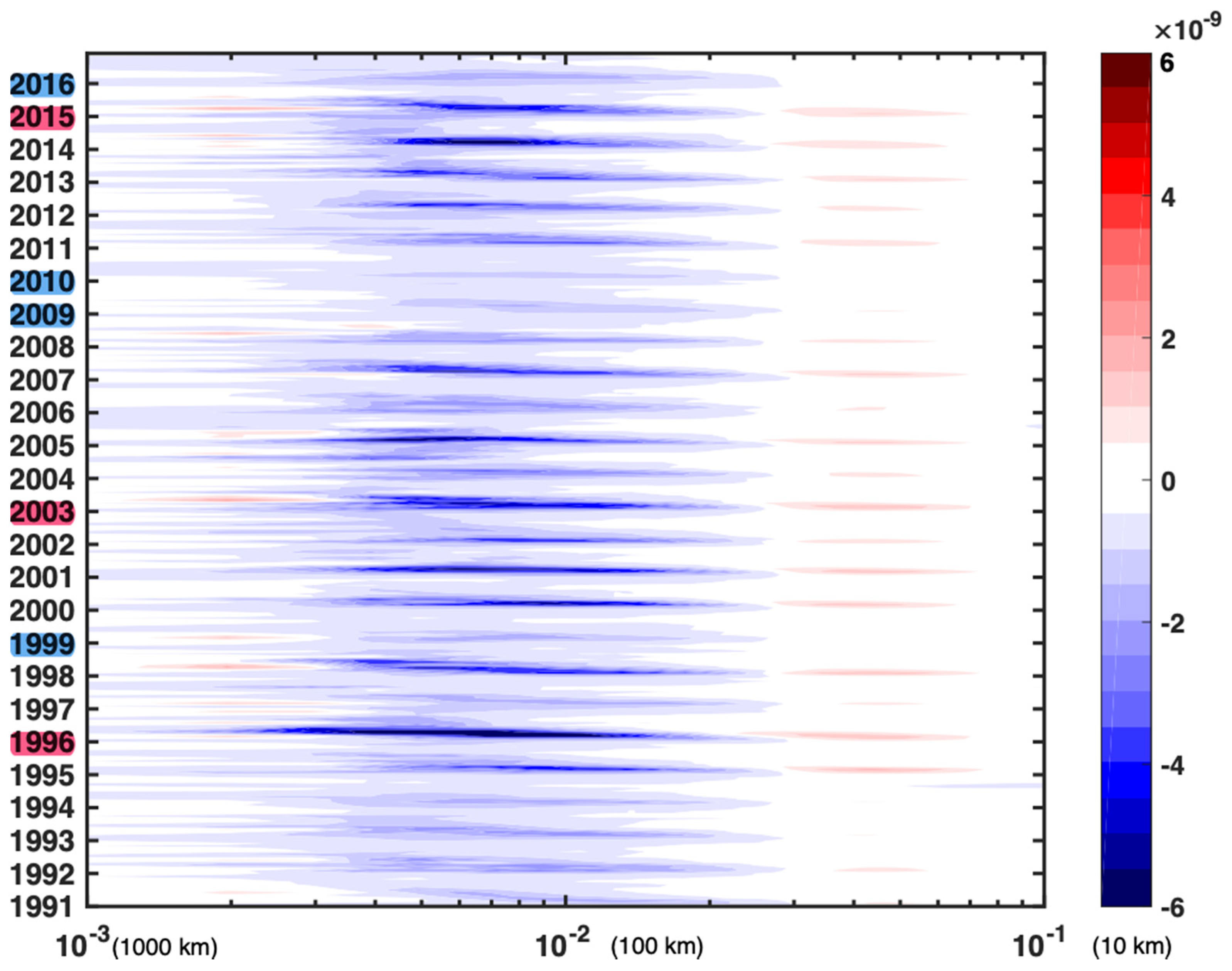
Figure 9 shows the time series of KE flux spectra in the STCC region. The seasonality of the spectra is distinct with large negative values in winter at the scales between 30 km and 200 km. These large negative values indicate the net upscale KE transfer, which is driven by the nonlinear interactions between eddies: the nonlinear merging between coherent eddies giving rise to larger ones occurs. At the submesoscales (<100 km), this inverse KE cascade enhances the mesoscale KE and subsequently the EKE. In the smaller scales (<30 km), the positive KE flux indicates the net downscale KE transfer, although this flux is much smaller than the negative flux at submesoscale. This downscale KE cascade may lead to the KE dissipation. These results show that the submesoscale KE enhanced by the MLI is transferred to both the larger and smaller scales, which are consistent with the previous studies [3,4].
The winter negative KE flux also varies on the timescales longer than interannual. The negative spectra magnitudes at the scale between 30 km and 100 km were large (<−3 × 10⁻⁹ m2 s−3) when the submesoscale KE was large in 1996, 2003, and 2015, and small (>−1.5 × 10⁻⁹ m2 s−3) when the submesoscale KE was small in 1999, 2009, 2010, and 2016 (Figure 4 and Table 1). Additionally, this inverse KE cascade appears to vary synchronously with submesoscale KE (red curve in Figure 8) on the decadal time scale, and also with EKE (black thin curve in Figure 2). The larger inverse KE cascade from the submesoscale possibly enhances the mesoscale KE and subsequently the EKE when the submesoscale KE is large. These results suggest that the possible impacts associated with the PDO to the MLD and buoyancy gradient modulate the EKE through the inverse KE cascade from the submesoscale to mesoscale.

3.5. Capture Capability of Submesoscale KE Variability by Argo Float Observations

We further examine the possibility that the conventional observations capture the variations of submesoscale motions demonstrated by OFES2_NP30 from estimation of the parameterized APE release at the coarse resolution. The monthly dataset of Grid Point Value of the Monthly Objective Analysis using the Argo data (MOAA GPV, [25]) is used, which is constructed by using the optimal interpolation method at a horizontal resolution of 1°. The monthly data from 2005 to 2016 are used because the Argo float observations started in 2000 and its number reached 75% of 3000 in 2005.
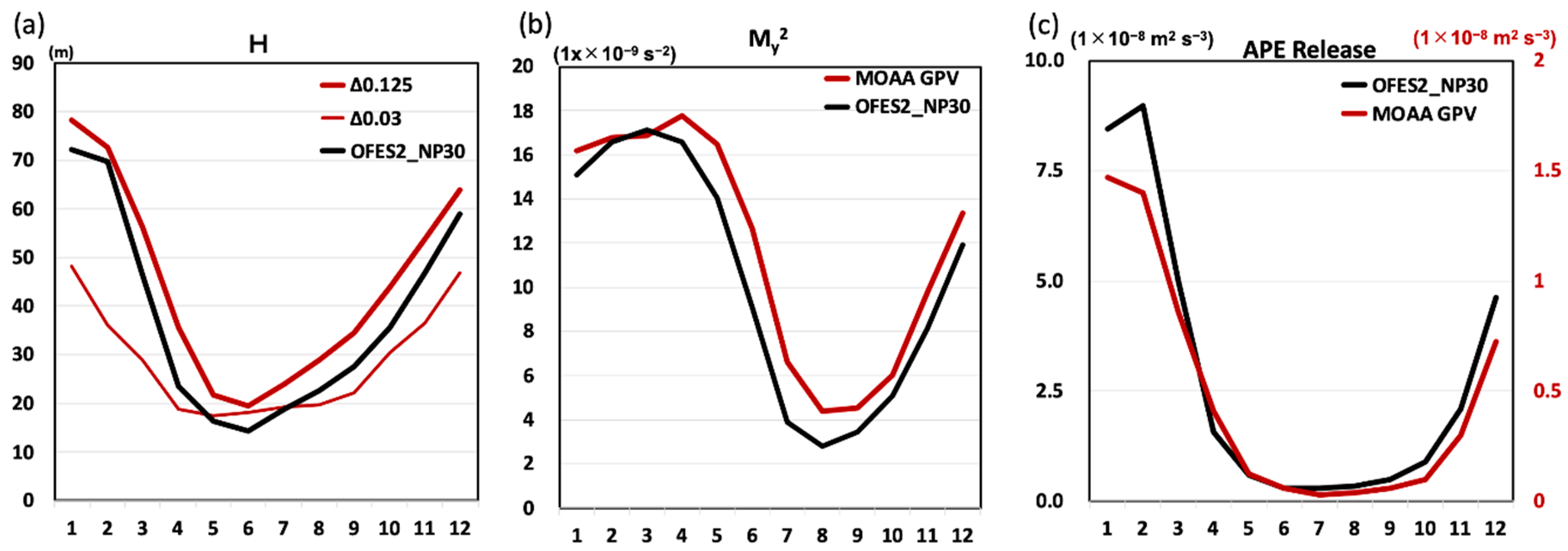
The monthly climatology of MLD in the STCC region varies seasonally, deep (>70 m) from January to February and shallow (<30 m) from May to July (H, thick curves in Figure 10a). The MLD in the MOAA GPV defined by the depth with a density change from the surface of 0.125 σθ (red thick curve) is comparable to that in OFES2_NP30 defined by the depth with a density change from the surface of 0.03 σθ (black curve). The MLD in MOAA GPV with the same definition of OFES2_NP30 (red thin curve) is too shallow. The reason is probably the coarse resolution of MOAA GPV that cannot capture the mesoscale and submesoscale motions. Therefore, the different definitions for MLD in MOAA GPV and OFES2_NP30 are used hereafter. Note that the period from January to February when the MLD is deep in the STCC region is earlier by about one and a half months than February to April in the North Pacific near the Kuroshio Extension, which is consistent with a previous study [26].
The surface meridional buoyancy gradient in the STCC region is large from January to April (>1.5 × 10⁻⁸ s−2) in both MOAA GPV and OFES2_NP30 (My2 in Figure 10b), although the large gradient in the MOAA GPV continues until May. The APE release in the STCC region also varies seasonally (Figure 10c). Both the APE releases in MOAA GPV and OFES2_NP30 are large from January to February and small from April to October. The APE release maximum in MOAA GPV (1.5 × 10⁻⁸ m2 s−3) is about one-sixth of that in OFES2_NP30 (9.0 × 10⁻⁸ m2 s−3), probably because of coarse horizontal resolution of MOAA GPV. In OFES2_NP30 the considerably large APE release is ubiquitous in the STCC region, but not in MOAA GPV (not shown). The seasonalities of the MLD, surface buoyancy gradient, and APE release in the STCC region are qualitatively similar between MOAA GPV and OFES2_NP30.
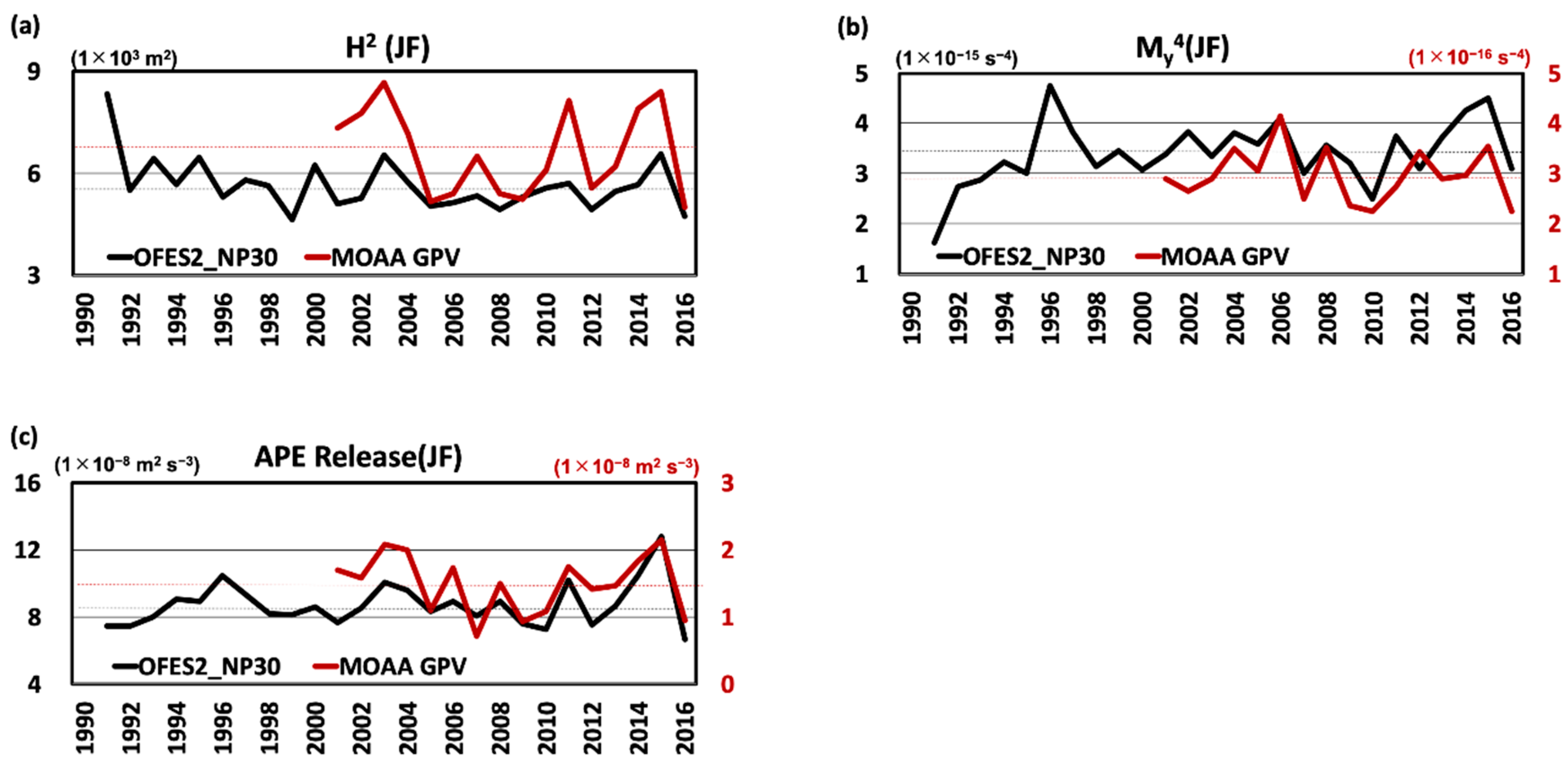
Next, we examine the interannual variations of MLD squared (H2), surface meridional buoyancy gradient squared (My4), and the APE release in winter in the STCC region. The interannual variations of the observed H2 in MOAA GPV are approximately similar to that of OFES2_NP30 (Figure 11a). Both were large in 2003, 2010, 2011, and 2015 and small in 2005, 2006, 2012, and 2016, which varied synchronously with each other with a high correlation value of 0.80. However, the standard deviation (SDV) in MOAA GPV is 1.28 × 10³ m2, which is more than two times of 5.3 × 10⁴ m2 in OFES2_NP30. On the other hand, the My4 in MOAA GPV varies less synchronously with that in OFES2_NP30 with a correlation value of 0.62, although both peak in 2006, 2011, and 2015, and bottom in 2005 and 2016. The SDV in MOAA GPV is 5.4 × 10⁻¹⁷ s−4, which is about one tenth of 5.2 × 10⁻¹⁶ s−4 in OFES2_NP30.
The APE release in winter in MOAA GPV varies synchronously with that in OFES2_NP30 with a high correlation value of 0.78. The average of the APE release in MOAA GPV (1.5 × 10⁻⁸ m2 s−3) is about one fifth of in OFES2_NP30 (8.8 × 10⁻⁸ m2 s−3) and its SDV (4.4 × 10⁻⁹ m2 s−3) is about one third of that (1.53 × 10⁻⁸ m2s−3) in OFES2_NP30. These small values in MOAA GPV are probably because of the estimation of the area average at the low-resolution of 1° as mentioned before: the ubiquitous patchy distribution of considerable large APE release in OFES2_NP30, but not in MOAA GPV. However, the high correlation of the APE releases suggests a possibility that the conventional observations can diagnose the interannual to decadal variations of the submesoscale KE in the STCC region.

4. Summary and Discussions

The interannual to decadal variations of the submesoscale KE in the STCC region were examined by using the outputs from a submesoscale permitting hindcast simulation in the North Pacific from 1990 to 2016. In addition to the seasonality of the submesoscale KE: large in winter and small in summer, the submesoscale KE were anomalously enhanced in 1996, 2003, and 2015, and reduced in 1999, 2009, 2010, and 2016. These variations are partially explained by the APE release in the process of the MLI, which is proportional to the product of the MLD squared and the horizontal buoyancy gradient squared. The large APE release enhances the submesoscale KE, and vice versa. The decadal variations also vary synchronously with the PDO. Both the MLD and horizontal buoyancy gradient variability in the STCC region appear to be associated with the PDO. On the other hand, the submesoscale KE is less influenced by either the MLD or the horizontal buoyancy gradient than the APE release. These results suggest that the interannual to decadal variations of submesoscale motions in the STCC region are induced by the MLI variations depending on both the MLD and buoyancy gradient.
The mesoscale KE (KE_M, blue curve) in the STCC region appears to vary synchronously with the submesoscale KE (KE_SM, red curve) on the interannual to decadal timescales (Figure 5). Both the peaks were anomalously large in 1996, 2003, and 2015, and small in 1999, 2009, 2010, and 2016. The relations between the PDO and the decadal variations of the mesoscale and submesoscale motions are suggested in Qiu and Chen (2013) [14] and this study, respectively. However, the instability mechanism inducing each motion is different from each other. The submesoscale motions are attributed to the MLI, but the mesoscale motions to the upper-ocean shear changes [14]. On the other hand, the inverse KE cascade from the submesoscale to the larger scale is another KE pathway (Figure 9). The large submesosocale KE enhances the inverse KE cascade and then the mesoscale KE is strengthened. These results show a possible pathway through submesoscale motions to explain the impact associated with the PDO on the mesoscale KE and EKE variability.
In this study, the submesoscale motions in the STCC region are attributed to the MLI and the APE release parameterized by Fox-Kemper et al. (2008) is used. However, this parameterized APE release does not fully explain the APE release directly estimated from the model outputs (see Figure 5 and Section 3.2). The other part should be revealed, which remains in the present study. For example, strain-induced frontogenesis [1,27] and turbulent thermal wind [28] are the candidates, which can induce the submesoscale motions. These drive the secondary circulation across the front and then lead to the APE release [27]. Although the OFES2_NP30 probably does not resolve these mechanisms due to its coarse resolution, further analyses of the existences of these mechanisms in the STCC region and their associated APE release are interesting topics. In addition, Torres et al. (2018) [29] suggested the existence of the submesoscale motions smaller than 50 km not related to internal waves. OFES2_NP30 also cannot resolve their scales adequately.
The relations between the variations of submesoscale motions and any other climate variabilities than the PDO cannot be excluded. In the years when the submesoscale KE is large (small), the SST is anomalously high (>0.4 °C) (low (<−0.4 °C)) in the central equatorial Pacific between 160° E and 160° W (Figure 7a) (160° E and 180° (Figure 7b)), which reminds us of El Niño Modoki [30]. The winter submesoscale KE in the STCC region varies synchronously with the El Niño Modoki index on the decadal timescales (Figure 8e). These suggest a possible contribution of El Niño Modoki to the variations of submesoscale motions in the STCC region. There are also possible contributions of the North Pacific Gyre Oscillation (NPGO) to the submesoscale motions in the STCC region (not shown) because of the distributions of the decadal SST variations resembling those of El Niño Modoki [31]. To clarify what climate variability is the most responsible for the submesoscale KE variations in the STCC region, a detailed examination using the long-term dataset should be needed, which remains as our future work.
Our study investigated the interannual to decadal variations of submesoscale motions in the STCC region. Our results suggested a possibility that the conventional observations of surface density and MLD such as the Argo float observations can capture part of the variations via the estimation of the APE release. To apply this method in the global ocean, the regionalities of oceanic fields should be considered. For example, based on the regional simulations, Capet et al. (2008) [32] showed that the APE release seasonality in the Argentinian shelf is mostly in phase with both the MLD and horizontal buoyancy gradient. On the one hand, Mensa et al. (2013) [2] using the regional simulation showed that the APE release seasonality in the Gulf Stream region is similar to that of the MLD, but not to the horizontal buoyancy gradient. To verify the method diagnosing the interannual to decadal variations of the winter submesoscale motions, the long-term observations capturing the submesoscale motions such as the forthcoming Surface Water and Ocean Topography (SWOT) altimeter mission [33] (https://swot.jpl.nasa.gov) are expected.

Author Contributions

Conceptualization, H.S.; methodology, H.S., B.Q., and P.K.; formal analysis, H.S., B.Q., and P.K.; investigation, H.S.; resources, H.S. and M.N.; data curation, H.S.; writing—original draft preparation, H.S.; writing—review and editing, B.Q., P.K., Y.S., and M.N.; visualization, H.S.; supervision, M.N.; project administration, M.N.; funding acquisition, M.N. All authors have read and agreed to the published version of the manuscript.

Funding

This research was funded by JSPS of Japan, Grant-in-Aid for Scientific Research on Innovative Areas 6102 (KAKENHI grant number JP19H05701).

Acknowledgments

OFES2_NP30 was conducted by using the Earth Simulator under the support of JAMSTEC. B.Q. acknowledges the support from NASA grant NNX17AH33G.

Conflicts of Interest

The authors declare no conflict of interest.

References

  1. McWilliams, J.C. Submesoscale currents in the ocean. Proc. R. Soc. A 2016, 472, 20160117. [Google Scholar] [CrossRef] [PubMed]
  2. Mensa, J.A.; Garraffo, Z.; Griffa, A.; Ozgokmen, T.M.; Haza, A.; Veneziani, M. Seasonality of the submesoscale dynamics in the Gulf Stream region. Ocean Dyn. 2013, 63, 923–941. [Google Scholar] [CrossRef]
  3. Sasaki, H.; Klein, P.; Qiu, B.; Sasai, Y. Impact of oceanic-scale interactions on the seasonal modulation of ocean dynamics by the atmosphere. Nat. Commun. 2014, 5, 5636. [Google Scholar] [CrossRef] [Green Version]
  4. Qiu, B.; Chen, S.; Klein, P.; Sasaki, H.; Sasai, Y. Seasonal mesoscale and submesoscale eddy variability along the North Pacific Subtropical Countercurrent. J. Phys. Oceanogr. 2014, 44, 3079–3098. [Google Scholar] [CrossRef] [Green Version]
  5. Callies, J.; Ferrari, R.; Klymak, J.M.; Gula, J. Seasonality in submesoscale turbulence. Nat. Commun. 2015, 6, 6862. [Google Scholar] [CrossRef] [Green Version]
  6. Boccaletti, G.; Ferrari, R.; Fox-Kemper, B. Mixed layer instabilities and restratification. J. Phys. Oceanogr. 2007, 37, 2228–2250. [Google Scholar] [CrossRef]
  7. Fox-Kemper, B.; Ferrari, R.; Hallberg, R. Parameterization of mixed layer eddies. Part I: Theory and diagnosis. J. Phys. Oceanogr. 2008, 38, 1145–1165. [Google Scholar] [CrossRef]
  8. Rocha, C.B.; Chereskin, T.K.; Gille, S.T.; Menemenlis, D. Mesoscale to submesoscale wavenumber spectra in Drake Passage. J. Phys. Oceanogr. 2016, 46, 601–620. [Google Scholar] [CrossRef]
  9. Qiu, B.; Chen, S.; Klein, P.; Wang, J.; Torres, H.; Fu, L.L.; Menemenlis, D. Seasonality in transition scale from balanced to unbalanced motions in the world ocean. J. Phys. Oceanogr. 2018, 48, 591–605. [Google Scholar] [CrossRef] [Green Version]
  10. Uda, M.; Hasunuma, K. The eastward subtropical countercurrent in the western North Pacific Ocean. J. Oceanogr. Soc. Jpn. 1969, 25, 201–210. [Google Scholar] [CrossRef] [Green Version]
  11. Qiu, B.; Koh, D.A.; Lumpkin, C.; Flament, P. Existence and formation mechanism of the North Hawaiian Ridge current. J. Phys. Oceanogr. 1997, 27, 431–444. [Google Scholar] [CrossRef]
  12. Yoshida, S.; Qiu, B.; Hacker, P. Low-frequency eddy modulations in the Hawaiian Lee Countercurrent: Observations and connection to the Pacific Decadal Oscillation. J. Geophys. Res. Oceans 2011, 116, C12009. [Google Scholar] [CrossRef] [Green Version]
  13. Mantua, N.J.; Hare, S.R.; Zhang, Y.; Wallace, J.M.; Francis, R.C. A Pacific interdecadal climate oscillation with impacts on salmon production. Bull. Am. Meteorol. Soc. 1997, 78, 1069–1079. [Google Scholar] [CrossRef]
  14. Qiu, B.; Chen, S. Concurrent decadal mesoscale eddy modulations in the western North Pacific subtropical gyre. J. Phys. Oceanogr. 2013, 43, 344–358. [Google Scholar] [CrossRef]
  15. Sasaki, H.; Kida, S.; Furue, R.; Aiki, H.; Komori, N.; Masumoto, Y.; Miyama, T.; Nonaka, M.; Sasai, Y.; Taguchi, B. A global eddying hindcast ocean simulation with OFES2. Geosci. Model Dev. Discuss. 2020. [Google Scholar] [CrossRef] [Green Version]
  16. Pacanowski, R.C.; Griffies, S.M. The MOM3 manual. In GFDL Ocean Group Tech. Rep. 4; NOAA. Geophysical Fluid Dynamics Laboratory: Princeton, NJ, USA, 1999. [Google Scholar]
  17. St. Laurent, L.C.; Simmons, H.L.; Jayne, S.R. Estimating tidally driven mixing in the deep ocean. Geophys. Res. Lett. 2002, 29, 2106. [Google Scholar]
  18. Noh, Y.; Kim, H.J. Simulations of temperature and turbulence structure of the oceanic boundary layer with the improved near-surface process. J. Geophys. Res. Oceans 1999, 104, 15621–15634. [Google Scholar] [CrossRef]
  19. Carrère, L.; Lyard, F.; Cancet, M.; Guillot, A.; Roblou, L. FES 2012: A new global tidal model taking advantage of nearly 20 years of altimetry. 20 Years Prog. Radar Altimetry 2012, 710, 13. [Google Scholar]
  20. Tsujino, H.; Urakawa, S.; Nakano, H.; Small, R.J.; Kim, W.M.; Yeager, S.G.; Danabasoglu, G.; Suzuki, T.; Bamber, J.L.; Bentsen, M.; et al. JRA-55 based surface dataset for driving ocean-sea-ice models (JRA55-do). Ocean Modell. 2018, 130, 79–139. [Google Scholar] [CrossRef]
  21. Large, W.; Yeager, S. Diurnal to decadal global forcing for ocean and sea-ice models: The data sets and flux climatologies. NCAR Technical Note NCAR/TN-460+STR 2004. [Google Scholar] [CrossRef]
  22. Zweng, M.M.; Reagan, J.R.; Antonov, J.I.; Locarnini, R.A.; Mishonov, A.V.; Boyer, T.P.; Garcia, H.E.; Baranova, O.K.; Johnson, D.R.; Seidov, D.; et al. World Ocean Atlas 2013, Volume 2: Salinity; Levitus, S., Technical, M.A., Eds.; NOAA Atlas NESDIS 74: Princeton, NJ, USA, 2013; p. 39. [Google Scholar]
  23. Zhai, X.; Greatbatch, R.J. Wind work in a model of the northwest Atlantic Ocean. Geophys. Res. Lett. 2007, 34, L04606. [Google Scholar] [CrossRef] [Green Version]
  24. Renault, L.; Marchesiello, P.; Masson, S.; McWilliams, J.C. Remarkable control of western boundary currents by eddy killing, a mechanical air-sea coupling process. Geophys. Res. Lett. 2019, 46, 2743–2751. [Google Scholar] [CrossRef] [Green Version]
  25. Hosoda, S.; Ohira, T.; Nakamura, T. A monthly mean dataset of global oceanic temperature and salinity derived from Argo float observations. JAMSTEC Rep. Res. Dev. 2008, 8, 47–59. [Google Scholar] [CrossRef] [Green Version]
  26. Ohno, Y.; Iwasaka, N.; Kobashi, F.; Sato, Y. Mixed layer depth climatology of the North Pacific based on Argo observations. J. Oceanogr. 2009, 65, 1–16. [Google Scholar] [CrossRef]
  27. Siegelman, L. Energetic submesoscale dynamics in the ocean interior. J. Phys. Oceanogr. 2020, 50, 727–749. [Google Scholar] [CrossRef] [Green Version]
  28. Gula, J.; Molemaker, M.J.; McWilliams, J.C. Submesoscale cold filaments in the Gulf Stream. J. Phys. Oceanogr. 2014, 44, 2617–2643. [Google Scholar] [CrossRef]
  29. Torres, H.S.; Klein, P.; Menemenlis, D.; Qiu, B.; Su, Z.; Wang, J.; Shen, S.; Fu, L.-L. Partitioning ocean motions into balanced motions and internal gravity waves: A modeling study in anticipation of future space missions. J. Geophys. Res. Oceans 2018, 123, 8084–8105. [Google Scholar] [CrossRef] [Green Version]
  30. Ashok, K.; Behera, S.K.; Rao, S.A.; Weng, H.; Yamagata, T. El Niño Modoki and its possible teleconnection. J. Geophys. Res. Oceans 2007, 112, C11007. [Google Scholar] [CrossRef]
  31. Di Lorenzo, E.; Cobb, K.; Furtado, J.; Schneider, N.; Anderson, B.T.; Bracco, A.; Alexander, M.A.; Vimont, D.J. Central Pacific El Niño and decadal climate change in the North Pacific Ocean. Nat. Geosci. 2010, 3, 762–765. [Google Scholar] [CrossRef]
  32. Capet, X.; Campos, E.J.; Paiva, A.M. Submesoscale activity over the Argentinian shelf. Geophys. Res. Lett. 2008, 35, L15605. [Google Scholar] [CrossRef] [Green Version]
  33. Fu, L.-L.; Ferrari, R. Observing oceanic submesoscale processes from space. Eos Trans. AGU 2008, 89, 488. [Google Scholar] [CrossRef]
Figure 1. Eddy kinetic energy (EKE) (log 10 cm2 s−2) estimated from the geostrophic currents of sea surface height (SSH) anomalies in the North Pacific based on (a) OGCM for the Earth Simulator version 2 (OFES2)_NP30 averaged over 1991–2016 and (b) satellite observations from AVISO (https://www.aviso.altimetry.fr) averaged over 1993–2016. The Subtropical Countercurrent (STCC) region (box region) is defined by the box region from 135° E to 165° E between 18° N and 28° N.
Fluids 05 00116 g001
Figure 2. Time series of daily mean (thick curves) and annual running mean (thin curves) EKE (cm2 s−2) in the STCC region in OFES2_NP30 (black curves) and the AVISO satellite observations (red curves). Qiu and Chen (2013) [14] showed that the EKE within the 18°–28° N in the Northwestern Pacific including the STCC and Hawaiian Lee Countercurrent (HLCC) were high in 1995–1998 and 2003–2006 (red arrows) and low in 1999–2002 and 2009–2011 (blue arrows).
Fluids 05 00116 g002
Figure 3. Surface relative vorticity (1×10⁻⁴ s−1) in the subtropical Northwestern Pacific on the day with maximum relative vorticity RMS in the STCC region (box area) in each year. The submesoscale motions are active in the left figures on (a) 17 March 1996, (b) 17 March 2003, and (c) 25 February 2015 and calm in the right figures on (d) 27 February 1999, (e) 1 April 2009, (f) 3 March 2010, and (g) 1 April 2016. The box region corresponds to the STCC region.
Fluids 05 00116 g003
Figure 4. Daily mean time series of surface relative vorticity RMS (black curve) and submesoscale KE (KE_SM, red curve) corresponding to surface kinetic energy with the scales smaller than 100 km in the STCC region. The left and right vertical axes show the scales of relative vorticity RMS and KE_SM respectively.
Fluids 05 00116 g004
Figure 5. Monthly time series of submesoscale KE (KE_SM, red curve), the parameterized available potential energy (APE) release (black curve), mesoscale KE (KE_M, blue curve), and the direct estimation (= w’b’, green curve) averaged within the mixed-layer depth (MLD) in the STCC region. The left vertical axis shows the scales of the KE_SM and the parameterized APE release and the right vertical axis shows the scales of the KE_M and w’b’. The factor three between the scales on the left and right vertical axes emphasized that the parameterized APE release is three times smaller than the APE release directly estimated from OFES2_NP30 outputs.
Fluids 05 00116 g005
Figure 6. (a) Annual time series of the submesoscale KE (KE_SM) averaged from February to April (red curve) and the parameterized APE release averaged from January to February (black curve) in the STCC region. Black curves indicate (b) meridional buoyancy gradient squared (My4) and (c) MLD squared (H2), respectively. Broken lines indicate the mean values.
Fluids 05 00116 g006
Figure 7. (a) Composite distributions of sea surface temperature (SST) anomalies averaged from January to February in 1996, 2003, and 2015 when submesoscale KE (KE_SM) in the STCC region was large. (b) is the same as (a), but in 1999, 2009, 2010, and 2016 when the KE_SM was small. (c,d) are the same as (a) and (b), respectively, but composite distributions of MLD anomalies. The box region corresponds to the STCC region.
Fluids 05 00116 g007
Figure 8. Time series of five-year running mean of submesoscale KE (KE_SM) averaged from February to April (red curve) and (a) parameterized APE release from January to February (black curve) in the STCC region. Black curves of (be) are the My4 and H2 in the STCC region, Pacific Decadal Oscillation (PDO) index (http://research.jisao.washington.edu/pdo/), and El Niño Modoki index (EMI) (http://www.jamstec.go.jp/frsgc/research/d1/iod/modoki_home.html.en) averaged from January to February respectively.
Fluids 05 00116 g008
Figure 9. Time series of surface spectral KE flux (Π in Equation (3), 1×10⁻⁹ m2 s−3) in the STCC region from 1991 to 2016. The submesoscale KE (KE_SM) is large (small) in the years with red (blue) shading in the vertical axis. Horizontal axis indicates wavenumber (cycle km−1). 10−3 cycle km−1, 10−2 cycle km−1, and 10−1 cycle km−1 correspond to the scales of 1000 km, 100 km, and 10 km, respectively.
Fluids 05 00116 g009
Figure 10. Monthly climatology of (a) MLD (H), (b) meridional buoyancy gradient (My2), and (c) parameterized APE release based on the Grid Point Value of the Monthly Objective Analysis using the Argo data (MOAA GPV) averaged from 2005 to 2016 (red curves) and OFES2 averaged from 1991 to 2016 (black curves). The MLD in MOAA GPV (red thick curves) and OFES2 (black curves) are defined by the depths with density changes from the surface of 0.125 σθ and 0.03 σθ, respectively. Another MLD in MOAA GPV with red thin curve in (a) is defined by the same as that in OFES2.
Fluids 05 00116 g010
Figure 11. Annual time series of (a) MLD squared (H2), (b) meridional surface buoyancy gradient squared (My4), and (c) parameterized APE release in winter averaged from January to February in the STCC region based on OFES2_NP30 (black curves) and MOAA GPV (red curves).
Fluids 05 00116 g011
Table 1. KE_SM anomaly averaged from February to April and the parameterized APE release, My4, and H2 anomalies averaged from January to February in 1996, 2003, and 2015 with enhanced submesoscale motions and in 1999, 2009, 2010, and 2016 with decayed submesoscale motions in the STCC region. The values with red and blue color are larger and smaller than the means, respectively.
1996200320151999200920102016Average
(1992–2016)
KE_SM (FMA) (1×10⁻³ m2s−2)0.971.260.99−0.8−0.84−1.15−1.473.43
APE Release(JF) (1×10⁻⁸ m2s−3)1.671.314.02−0.65−1.2−1.54−2.18.76
My4 (JF) (1×10⁻¹⁵ s−4)1.28−0.131.03−0.03−0.27−0.99−0.383.47
H2(JF) (1×10³ m)−0.261.001.02−0.91−0.250.03−0.815.54
Notes: The values with red and blue color are larger and smaller than the means, respectively.

