Verification and Validation of openInjMoldSim, an Open-Source Solver to Model the Filling Stage of Thermoplastic Injection Molding

Abstract

In the present study, the simulation of the three-dimensional (3D) non-isothermal, non-Newtonian fluid flow of polymer melts is investigated. In particular, the filling stage of thermoplastic injection molding is numerically studied with a solver implemented in the open-source computational library $OpenFOA{M}^{\circledR }$. The numerical method is based on a compressible two-phase flow model, developed following a cell-centered unstructured finite volume discretization scheme, combined with a volume-of-fluid (VOF) technique for the interface capturing. Additionally, the Cross-WLF (Williams–Landel–Ferry) model is used to characterize the rheological behavior of the polymer melts, and the modified Tait equation is used as the equation of state. To verify the numerical implementation, the code predictions are first compared with analytical solutions, for a Newtonian fluid flowing through a cylindrical channel. Subsequently, the melt filling process of a non-Newtonian fluid (Cross-WLF) in a rectangular cavity with a cylindrical insert and in a tensile test specimen are studied. The predicted melt flow front interface and fields (pressure, velocity, and temperature) contours are found to be in good agreement with the reference solutions, obtained with the proprietary software $Moldex3D^{\circledR }$. Additionally, the computational effort, measured by the elapsed wall-time of the simulations, is analyzed for both the open-source and proprietary software, and both are found to be similar for the same level of accuracy, when the parallelization capabilities of $OpenFOA{M}^{\circledR }$ are employed.

1. Introduction

The ever-growing demand for plastic materials promoted an increase in the requirements of many transformation processes, as happens for injection molding (IM), which is currently the most used one to manufacture thermoplastic parts. IM allows producing parts with a wide range of geometries and presents a return on investment in the medium/long term. Moreover, this transformation process presents a high fixed cost, not only due to the molds used, but also due to the many process variables that are necessary to control and optimize, to achieve the optimal processing conditions. It is exactly due to these requirements that simulation started to gain more importance in IM, being currently an indispensable step in the design phase to, among others, minimize the amount of experimental iterations needed to manufacture a tool, to decrease the overall cost of development, and to be able to produce parts with the desired geometrical and mechanical requirements.

There are several proprietary software solutions available for the simulation of the IM process and related techniques [1]. However, in addition to the expensive licenses, the proprietary software usually cannot be adapted to specific user needs, thus preventing the access of small to medium sized companies to these tools. Open-source free alternatives may allow turning around these limitations, and, additionally, one can have access and adapt the source code. In the broad area of computational fluid dynamics (CFD), $OpenFOA{M}^{\circledR }$ [2] became a very interesting alternative to proprietary software, due to the range of available continuum mechanics solvers and an active development community.

In what concerns to polymer processing, $OpenFOA{M}^{\circledR }$ [2] has been used in different areas like extrusion, blow molding, and to some extent, injection molding. In the extrusion area, many $OpenFOA{M}^{\circledR }$ [2] based tools are already available; for example, the work in Habla et al. [3] presented the development and validation of a model to compute the temperature distribution in the calibration stage of extruded profiles. Later, the work in Rajkumar et al. [4] presented design guidelines to support die designers to obtain balanced flow distributions. For the numerical modeling of IM, Araújo et al. [5] provided a parallel 3D unstructured non-isothermal flow solver, with both polymer and air being considered as incompressible fluids. Their results presented a good accuracy and reasonable parallel efficiency and scalability. Making use of the $OpenFOA{M}^{\circledR }$ [2] computational library, the work in Nagy and Steinbichler [6] introduced a framework of a compressible two-phase (air and polymer melt) fluid model, with polymer-specific material models, for the description of the filling, packing, and cooling stages. Although for simple geometries, they proved that the framework of solving the compressible form of continuity, linear momentum, and energy equations resulted in a good agreement between experimental observations and theoretical predictions. Other researchers also tried to succeed in this task. Magalhães [7] in her Master Thesis implemented the energy equation, as well as the Bird–Carreau rheological model in the $interFoam$ solver available in the $OpenFOA{M}^{\circledR }$ [2] CFD library. She studied the filling stage of the IM process and implemented a boundary condition, which allowed the air to escape from the cavity, but not the polymer, as happens in real-life molds. With the use of that boundary condition in the numerical simulations, she concluded that a higher percentage of filled cavity was obtained. She also showed that differences in polymer and air viscosities were some of the main reasons for the large number of instabilities observed in the numerical calculation procedure. Recently, also aiming to model the IM process, the works in Mole et al. [8] and Krebelj and Turk [9] implemented both the Cross-WLF and modified Tait models in the $compressibleInterFoam$ (a solver designated by $openInjMoldSim$). The objective was to simulate the filling and packing stages, considering compressible flow, and applying appropriate models for the polymeric materials’ behavior. The solver was validated with a simple 2D demo test case for an amorphous polystyrene grade. Subsequently, Fontaínhas [10] in her Master Thesis used the $openInjMoldSim$ solver with a 3D case study (a simple thin rectangular geometry) and compared the results predicted by the solver (velocity, pressure, and temperature profiles) with the ones obtained by the proprietary software $Moldex3D^{\circledR }$[11]. A mesh sensitivity analysis was performed, and she reached the conclusion that the results predicted with the $openInjMoldSim$ solver were qualitatively similar to the ones obtained with $Moldex3D^{\circledR }$ [11]. However, the results obtained with the mesh refinement study did not converged to a level of accuracy with statistical significance. She also reported that the open-source solver was 18 times slower than the proprietary one.

This work describes the numerical validation of an open-source solver, $openInjMoldSim$ [8,9], able to simulate the filling stage of the thermoplastic IM process. For that purpose, mesh sensitivity studies were performed for all the validation case studies. This way, accurate/converged solutions were obtained for all the flow fields, which could not be found in preliminary studies performed with the same numerical algorithm. For that purpose, we used the Richardson extrapolation technique to estimate the discretization error. Additionally, to the best of the authors’ knowledge, this was the first time that compressible and incompressible formulations were compared, and the effect of the artificial interface compression term was assessed for the IM filling stage. Finally, to conclude about the novel contributions of the present work, the studies performed provided a detailed comparison of open-source and proprietary software, in terms of accuracy and performance.

This paper is organized in the following manner: In Section 2, we present the mathematical formulation of the modeling code that is used in this work, including the governing equations and numerical discretization. In Section 3, we present a number of case studies involving the filling of cavities with Newtonian and generalized Newtonian fluids. In each case study, a comparison of the results obtained with $openInjMoldSim$ is performed with data reported in the literature and obtained with the proprietary software $Moldex3D^{\circledR }$ [11], in order to assess its accuracy, robustness, and performance. Finally, in Section 4, we summarize the main conclusions of this work.

2. Mathematical Formulation

In this section, we present the mathematical formulation for an algorithm that is able to handle the polymer melt filling stage of the IM process efficiently. Contrarily to the commonly used assumption of fluids’ incompressibility [12], the employed algorithm considers a compressible, non-isothermal based formulation, which, in the future, will provide a rigorous basis for the simulation of the packing and cooling stages. The implementation was performed in the open-source framework code $OpenFOA{M}^{\circledR }$ [2,9].

2.1. Governing Equations

In the approach employed, the air and the polymer melt phases are assumed to be immiscible and compressible, unless otherwise stated. During the filling stage, the flow is governed by the mass, momentum, and energy conservation equations, which can be written as follows [1]:

$$\begin{array}{c}\hfill \frac{\partial \rho }{\partial t}+\nabla ·\left(\rho \mathbf{u}\right)=0,\end{array}$$

(1)

$$\begin{array}{c}\hfill \frac{\partial \left(\rho \mathbf{u}\right)}{\partial t}+\nabla ·\left(\rho \mathbf{u}\mathbf{u}\right)=\nabla ·\sigma ,\end{array}$$

(2)

$$\begin{array}{c}\hfill \frac{\partial \left(\rho c_{P}T\right)}{\partial t}+\nabla ·\left(\rho c_P\mathbf{u}T\right)=\beta T\left(\frac{\partial p}{\partial t}+\mathbf{u}·\nabla p\right)+p\nabla ·\mathbf{u}+\sigma :\nabla \mathbf{u}+\nabla ·\left(k\nabla T\right),\end{array}$$

(3)

where $\mathbf{u}$, p, and T denote the velocity vector, pressure, and temperature fields, respectively, t is the time, and $\sigma$ is the total, or Cauchy, stress tensor. The parameters $\rho$, $\beta$, $c_P$, and k represent the fluid density, compressibility coefficient, specific heat capacity, and thermal conductivity, respectively. The Cauchy stress tensor is given by:

$$\begin{array}{c}\hfill \sigma =-p\mathbf{I}+\mathsf{\tau },\end{array}$$

(4)

where $\mathbf{I}$ is the identity tensor and $\mathsf{\tau }$ is the extra or deviatoric stress tensor, which, for the flow of a compressible generalized Newtonian fluid, is defined as:

$$\begin{array}{c}\hfill \mathsf{\tau }=2\eta \left(T,p,\dot{\gamma }\right)\mathbf{D}-\frac{2}{3}\eta \left(T,p,\dot{\gamma }\right)\left(\nabla ·\mathbf{u}\right)\mathbf{I},\end{array}$$

(5)

where $\dot{\gamma }=\sqrt{2(\mathbf{D}:\mathbf{D})}=\sqrt{2\mathrm{tr}\left({\mathbf{D}}^2\right)}$ is the generalized shear rate, with $\mathbf{D}$ being the deformation rate tensor defined as $\mathbf{D}=(\nabla \mathbf{u}+{(\nabla \mathbf{u})}^T)/2$, and $\eta \left(T,p,\dot{\gamma }\right)$ is the fluid viscosity, which is considered to be a function of T, p and $\dot{\gamma }$ (see Section 2.1.1 for detailed information about the rheological models used in this work).

The simulation of the IM filling stage requires solving the fluid flow equations and capturing the melt front location at every time step. For that purpose, an advanced free-surface capturing model [13], based on the volume-of-fluid (VOF) method [14] is used. In this method, a species transport equation is used to track the relative volume fraction of the two phases, or phase fraction, $\alpha$, distribution. The phase fraction ranges from zero to one, zero being for air and one for the polymer melt. In this way, the fluid interface is located in regions where 0 $<\alpha <$ 1, and the physical properties can be calculated as an average weighted by $\alpha$, as follows:

$$\psi ={\psi }_m\alpha +{\psi }_a\left(1-\alpha \right),$$

(6)

where the subscripts m and a denote the melt and air phases’ properties, respectively, and $\psi$ represents all the relevant fluid properties, namely $\rho$, $\eta$, $c_P$, and k. The governing equation for the phase fraction, $\alpha$, is defined as:

$$\begin{array}{c}\hfill \frac{\partial \alpha }{\partial t}+\nabla ·\left(\alpha \mathbf{u}\right)+\nabla ·\left[\alpha (1-\alpha ){\mathbf{u}}_r\right]=S_p+S_u,\end{array}$$

(7)

where ${\mathbf{u}}_r$ is the relative velocity vector, commonly denominated by “compression velocity”. In this work, the compression velocity is given by:

$${\mathbf{u}}_r={\mathbf{n}}_{f}min\left[C_{\alpha }\frac{\left|\varphi \right|}{\left|{\mathbf{S}}_f\right|},max\left(\frac{\left|\varphi \right|}{\left|{\mathbf{S}}_f\right|}\right)\right],$$

(8)

where $\varphi$ is the volume flux at faces, ${\mathbf{S}}_f$ is the face normal vector pointing outwards from the cell, and $C_{\alpha }$ is an adjustable coefficient that determines the magnitude of the compression (usually $C_{\alpha }⩾1$) [15]. ${\mathbf{n}}_f$ is the interface unit normal vector taken from the phase fraction distribution as:

$${\mathbf{n}}_f=\frac{{\left(\nabla \alpha \right)}_f}{\left|{\left(\nabla \alpha \right)}_f+\delta \right|},$$

(9)

where $\delta$ is a stabilization factor [15].

The artificial interface compression term is an extra term added to the phase fraction evolution equation and is non-zero only when $0<\alpha <1$, i.e., at the fluid interface, and avoids its numerical diffusion (notice that in reality, the two fluid flow presents a sharp interface) [16]. Otherwise, a significant diffusion of $\alpha$ at the interface region might occur, predicting a nonphysical smeared interface, especially with coarse meshes. $S_p$ and $S_u$ represent two terms that arise from considering a compressible material [16]. Detailed information about the advanced free-surface capturing model used in this work can be found in Berberović et al. [13].

2.1.1. Constitutive Models

The rheological behavior of the melt and air phases is defined by a single-fluid two-phase model, where the average kinematic viscosity is given by Equation (6), in which $\psi$ is replaced by the viscosity $\eta$. For the air phase, the kinematic viscosity is assumed to be constant, i.e., a Newtonian fluid. For the polymer melt, the Cross-WLF constitutive model is employed. This constitutive model is widely adopted for studying both the filling and packing stages of the IM process [17] and is given by:

$$\begin{array}{c}\hfill {\eta }_m\left(T,p,\dot{\gamma }\right)=\frac{{\eta }_0\left(T,p\right)}{1+{\left({\eta }_0\left(T,p\right)\dot{\gamma }/{\tau }^{*}\right)}^{1-n}},\end{array}$$

(10)

where ${\tau }^{*}$ is the material constant representing the shear stress, above which the pseudoplastic behavior of the melt is observed, n is the power-law index, and ${\eta }_0\left(T,p\right)$ is the viscosity at the null shear rate. In this work, we adopted the Williams–Landel–Ferry (WLF) model [18] to describe the dependence of ${\eta }_0$ on T and p, given by:

$$\begin{array}{c}\hfill {\eta }_0\left(T,p\right)=D_1\exp \left[\frac{-C_1\left(T-T_0\right)}{C_2+T-T_0}\right],\end{array}$$

(11)

where $T_0=D_2+D_{3}p$ and $D_1$, $D_2$, $D_3$, $C_1$, and $C_2$ are parameters determined by experimental characterization [6].

2.1.2. Equation of State

Polymers shrink when pressure increases; thus, their specific volume (the reciprocal of the density) decreases [19]. On the other hand, with the increase of temperature, polymeric materials tend to expand, and, consequently, their specific volume increases. The relation of specific volume, pressure, and temperature is designated by the pressure-volume-temperature behavior (PVT) [20]. The most commonly used model to characterize the material PVT behavior of polymer melts is the modified Tait model [21], because it can describe properly the PVT relation of both amorphous and semi-crystalline polymers [19]. In the modified Tait model, the specific volume, $\hat{V}$, is given by:

$$\begin{array}{cc}\hfill \hat{V}& =\widehat{V_0}\left[1-Cln\left(1+\left(\frac{p}{B}\right)\right)\right]+\widehat{V_t},\hfill \end{array}$$

(12)

where:

$$\begin{array}{cc}\hfill \widehat{V_0}& =\left\{\begin{array}{c}{b}_{1S}+b_{2S}\left(T-b_5\right),\mathrm{if}T\le T_t\hfill \\ b_{1L}+b_{2L}\left(T-b_5\right),\mathrm{if}T>T_t\hfill \end{array}\right.,\hfill \end{array}$$

(13)

$$\begin{array}{cc}\hfill B& =\left\{\begin{array}{c}{b}_{3S}exp\left(-b_{4S}\left(T-b_5\right)\right),\mathrm{if}T\le T_t\hfill \\ b_{3L}exp\left(-b_{4L}\left(T-b_5\right)\right),\mathrm{if}T>T_t\hfill \end{array}\right.,\hfill \end{array}$$

(14)

$$\begin{array}{cc}\hfill \widehat{V_t}& =\left\{\begin{array}{cc}{b}_{7}exp\left(b_8\left(T-b_5\right)-b_{9}p\right),\hfill & \mathrm{if}T\le T_t\hfill \\ 0,\hfill & \mathrm{if}T>T_t\hfill \end{array}\right.,\hfill \end{array}$$

(15)

where $C=0.0894$ is a dimensionless constant, the coefficients $b_1$ to $b_9$ are obtained by fitting experimental characterization data, and p and T are the material pressure and temperature, respectively [19]. The subscripts S, L, and t represent solid, liquid (or melt), and transition states, respectively. The transition temperatures for semi-crystalline and amorphous polymers are the melt ($T_m$) and glass ($T_g$) transition temperatures, respectively.

The equation of state employed for the air phase is the ideal gas equation given by:

$$\rho =\frac{p}{RT},$$

(16)

where R is the ideal gas constant ($R=8.314$ J/(K.mol)).

2.2. Numerical Discretization

The numerical solution of the equations presented in Section 2.1 relies on a collocated finite volume method (FVM) approach, which uses the conservative integral forms of the governing equations for the single-fluid two-phase model [22]. The implementation of the three conservation equations (continuity, momentum, and energy) is done using the $OpenFOA{M}^{\circledR }$ computational library [2,23]. For more details about the solver employed in this work, the reader is referred to Mole et al. [8] and Krebelj and Turk [9].

3. Validation Case Studies

This section presents the case studies employed for the validation of the solver applied to the filling stage of the IM process ($openInjMoldSim$) presented in Section 2. The first case study was devoted to the flow along a cylindrical channel, in which the fluid was considered to have Newtonian rheology. The objective was to make a comparison of the obtained numerical velocity and pressure fields with an analytical solution available for steady-state conditions [24]. In the second case study, an assessment of the effect of the material compressibility in the filling stage of the IM process, in a rectangular cavity with a cylindrical insert, is presented. Finally, a detailed comparison between openInjMoldSim and Moldex3D^® [11] was performed in a more complex geometry, the cavity of a mold employed to manufacture tensile test specimens, a part representative of the typical ones produced by the IM process, which was used for material mechanical characterization purposes [24,25].

In all case studies considered in this work, the domain was divided into inlet, outlet, and boundary walls. Moreover, a fixed velocity was imposed at the inlet boundary patch, and at the same location, the homogeneous Neumann boundary condition was applied for the pressure field. Additionally, the no-slip velocity was imposed at the cavity walls. Furthermore, the walls only experience heat flux modeled by heat convection. Since the initial and boundary conditions were similar for all case studies, for organization purposes,

Table 1. Initial and boundary conditions for all case studies.

	Temperature (T)	Velocity (U)	Pressure (P)	Phase Fraction ($\mathit{\alpha }$)
Inlet	230 ${}^{°}$C	$U_{in}$	Null normal gradient	1
Outlet	Null normal gradient	Null normal gradient	105 Pa (atmospheric)	Null normal gradient
Walls	Heat convection Tmold = 50 ${}^{°}$C h = 1250 W/(m2. K)	Null velocity	Null normal gradient	Null normal gradient
Initial Condition	230 ${}^{°}$C	Null velocity	105 Pa (atmospheric)	0

shows the default initial and boundary conditions for all case studies. The particularities of each case study will be presented in the respective subsection.

The material used in the simulations was the GPPS (general purpose polystyrene) Styron 678, from Americas Styrenics. The rheological model employed was the Cross-WLF presented in Section 2, and its parameters are given in

Table 2. Cross-WLF coefficients for GPPS (general purpose polystyrene) Styron 678 from Americas Styrenics [11].

Parameter	Value
n	0.2903
${\tau }^{*}\left(\mathrm{Pa}\right)$	13,678
$D_1\left(\mathrm{Pa}.\mathrm{s}\right)$	7.44 × 10${}^{10}$
$D_2\left(\mathrm{K}\right)$	373.15
$D_3\left(\mathrm{K}/\mathrm{Pa}\right)$	0.0
$A_1$	25.971
$A_2\left(\mathrm{K}\right)$	51.6

. These parameters were obtained from the $Moldex3D^{\circledR }$ [11] materials database. The variation of viscosity with shear-rate, temperature, and pressure is given in Figure 1, which shows that the viscosity of the polymer melt decreases with the increase of both the shear-rate and the temperature.

As stated before, the air was assumed to be a Newtonian fluid by making use of the Newtonian rheological model, and by setting a dynamic viscosity equal to 0.1 Pa.s. Additionally, the thermodynamic properties, specific heat capacity, $c_p$, and thermal conductivity, k, were defined as 1007 J/(kg.K) and $0.0263$ W/(m.K), respectively, for the air and 2100 J/(kg.K) and $0.15$ W/(m.K), respectively, for the polymer melt.

The PVT behavior of the material was modeled using the modified Tait model, illustrated in Figure 2. The compressibility model adopted show that the specific volume of the material decrease with the increase of pressure, and increase with the increase of temperature following a slope until T_g (glass transition temperature) is reached. After T_g, the slope increases (as is commonly observed in amorphous polymers).

The coefficients of the modified Tait model are shown in

Table 3. Modified Tait model coefficients for the GPPS Styron 678 from Americas Styrenics [11].

Parameters	Compressible Formulation
$b_{1m}$ (m${}^3$/kg)	0.0009881
$b_{2m}$ (m${}^3$/(kg.K))	7.03 × 10${}^{-7}$
$b_{3m}$ (Pa)	1.71 × 10${}^8$
$b_{4m}$ (1/K)	0.004495
$b_{1s}$ (m${}^3$/kg)	0.0009873
$b_{2s}$ (m${}^3$/(kg.K))	2.89 × 10${}^{-7}$
$b_{3s}$ (Pa)	2.43 × 10${}^8$
$b_{4s}$ (1/K)	0.003106
$b_5$ (K)	373.98
$b_6$ (K/Pa)	2.88 × 10${}^{-7}$
$b_7$ (m${}^3$/kg)	0
$b_8$ (1/K)	0
$b_9$ (1/Pa)	0

. These coefficients were obtained from the $Moldex3D^{\circledR }$ materials database [11].

In the analysis of the case studies presented below, the methodologies used are common to more than one case study. Therefore, for organization purposes, the methods for assessment and verification used are presented here:

IC and NIC variations: The abbreviation “IC” stands for interface compression, which means that the artificial interface compression term of Equation (7) is considered, and the abbreviation “NIC” stands for the simulation where it was neglected.

Switch-over time: The time for the polymer melt to reach the switch-over position. This is an important instant for the analysis of the numerical calculation, since it coincides with the transition of the filling to the packing/holding stages. Assuming incompressibility, the equation to calculate the time the polymer melt takes to reach the switch-over point, $t_{SO}$, is given by:

$$t_{SO}=\frac{V}{A\times U_{in}},$$

(17)

where $U_{in}$ is the imposed average velocity at the inlet face, A the area of the inlet face, and V the volume at the switch-over point. In all the case studies presented, the switch-over point was assumed to occur when 98% of the total cavity volume is filled, which is a value commonly employed in the IM process [26].

Average properties: For assessment purposes, throughout the three case studies, minimum, average, and maximum properties were calculated. Considering a number of cells n, the average values are given by:

$$\overline{\theta }=\sum _{i=1}^n\frac{\left(\left|C_i\right|\times {\theta }_i\right)}{\left|C_i\right|},$$

(18)

where $\left|C_i\right|$ can be either the cell face area, when analyzing a cross-section, or the cell volume, when analyzing all the geometry. When $\left|C_i\right|$ is constant Equation (18) becomes the arithmetic mean.

Richardson’s extrapolation (RE): This is a widely employed method to estimate discretization errors [27]. It can be applied to any discretization procedure, either for differential or integral governing equations, such as the FVM [28]. This method was used in this work to extrapolate the value of the variable under analysis to an infinitely refined mesh and, thus, allowed estimating the accuracy of the results at each level of mesh refinement. For a detailed description of this technique see Appendix A.

3.1. Case Study 1: Filling of a Cylindrical Cavity

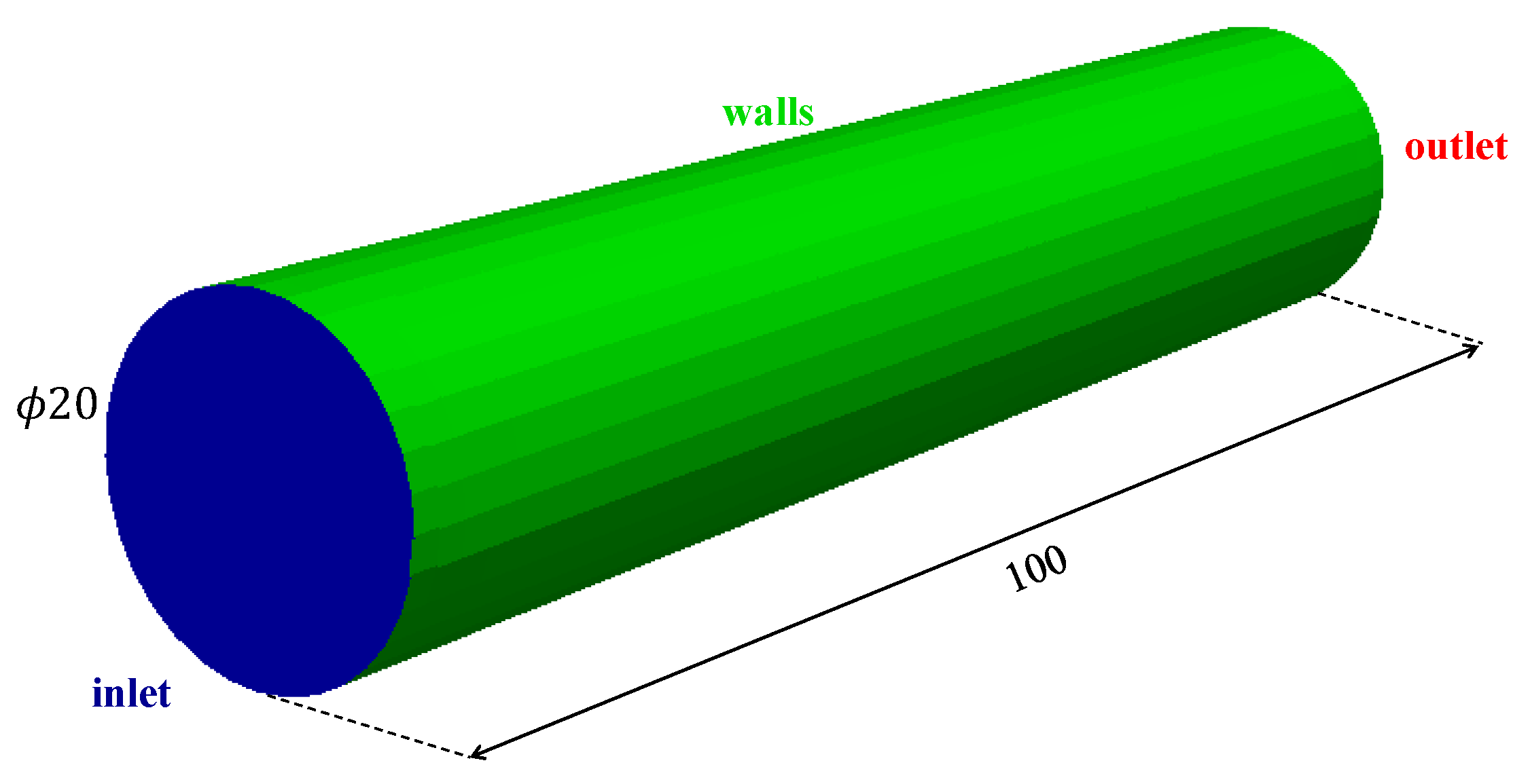
This first case study covered the flow of a Newtonian fluid along a cylindrical channel and was used to verify if the numerical algorithm was properly implemented. The cavity geometry employed in this first case study is illustrated in Figure 3.

The initial and boundary conditions used in this case study are presented in Table 1, with an inlet velocity of $U_{in}$ = 4 m/s.

The mesh sensitivity analysis was undertaken with three levels of refinement, where the number of cells of the coarsest mesh (M1) was doubled in each direction to obtain the second degree of refinement (M2). The same procedure was applied to obtain the most refined level (M3). The software $cfMesh$ [29] was used to generate the three meshes, which had 4368, 34,280, and 263,016 cells for M1, M2, and M3, respectively.

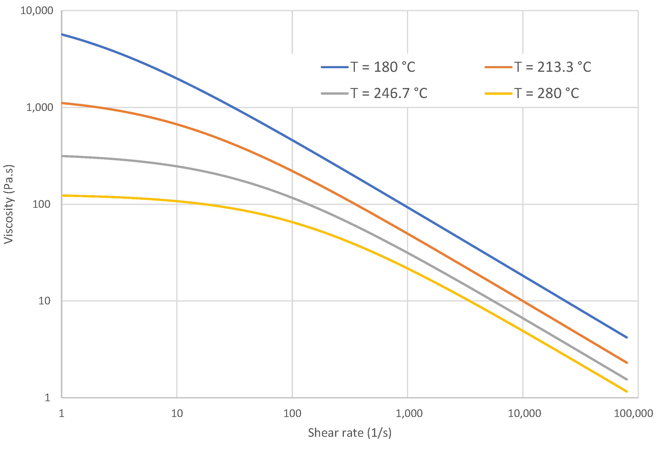
The polymer melt was considered to behave as a Newtonian fluid, with a dynamic viscosity value of 310.0 Pa.s, obtained by using $n=1$ in the Cross-WLF rheological model presented in Section 3. The thermodynamic properties of the air and polymer melt are also the ones presented in Section 3.

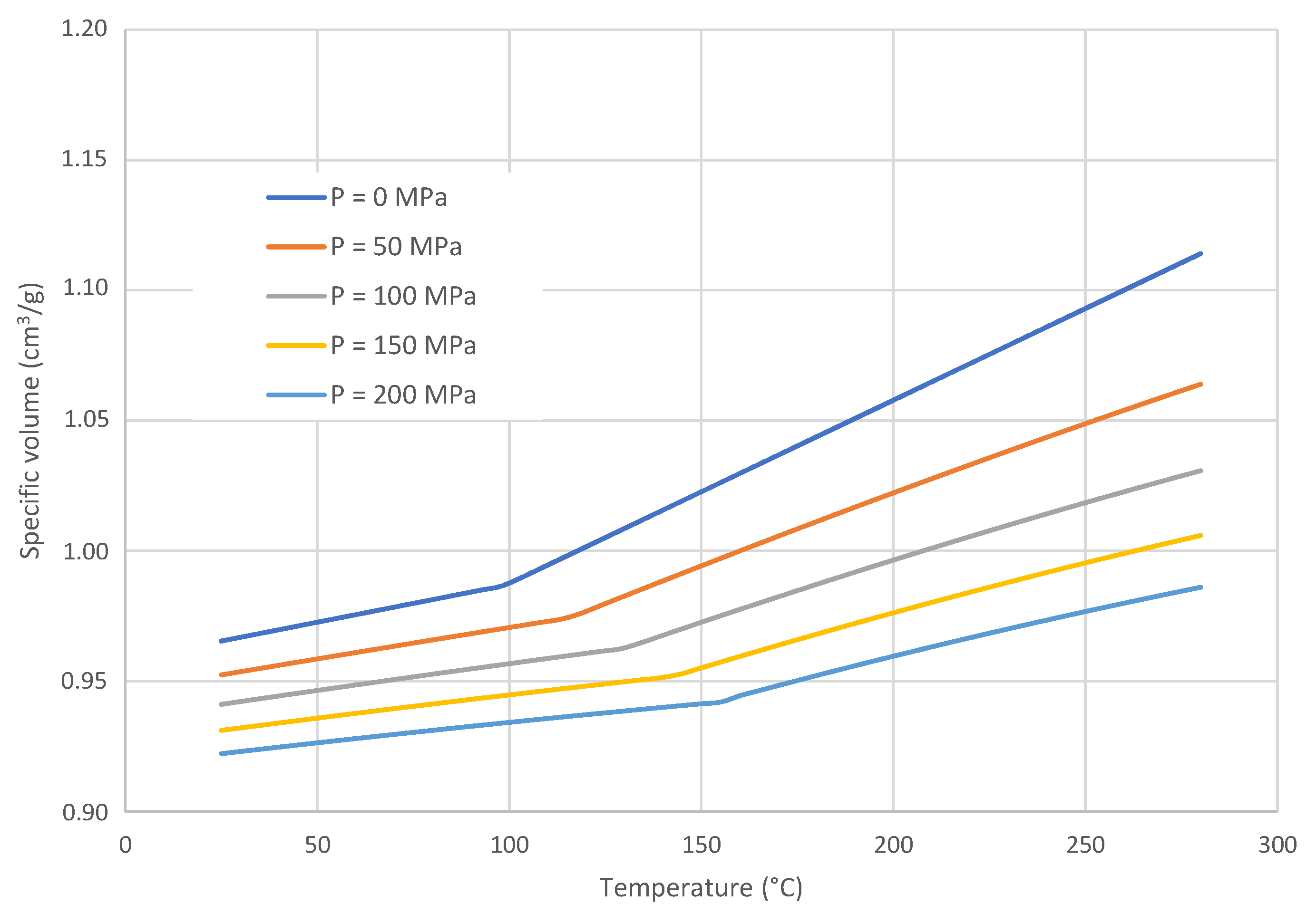
The PVT behavior of the material was prescribed using two formulations, the compressible one, given by the modified Tait model, which was already shown in Figure 2 and Table 3, and the incompressible, where the melt density employed was constant and equal to 1.075 g/cm${}^3$.

The first tests carried out were related to the time predicted by the algorithm to achieve the switch-over point, $t_{SO}$, for the incompressible formulation and to compare it with the theoretical value calculated from Equation (17). The results obtained are given in

Table 4. Comparison of the switch-over time obtained for the incompressible formulation, considering both interface compression (IC) and neglecting IC (NIC) variations. The analytical reference value calculated from Equation (17) is $t_{SO}=0.0245$ s.

Mesh	IC		NIC
	${\mathit{t}}_{\mathbf{SO}}$ (s)	Error (%)	${\mathit{t}}_{\mathbf{SO}}$ (s)	Error (%)
M1	0.0249	1.630	0.0462	88.60
M2	0.0246	0.408	0.0250	2.040
M3	0.0230	6.120	0.0247	0.816

for both the IC and NIC variations.

From the data shown in Table 4, one can conclude that the IC gave accurate results for coarse and medium meshes, because it minimizes the effect of the interface diffusion and, therefore, favors the mass conservation. Since NIC omits the contribution of the artificial interface compression, the results deviated from the analytical values, especially for the coarsest mesh (M1). On the other side, with refined meshes, neglecting the artificial diffusion term did not affect the mass balance. In a future work, a detailed study should allow identifying the criteria related to the necessity of considering the interface compression term in these simulations.

To understand the differences caused by considering the polymer melt as incompressible, and since the compressible formulation was the most realistic one,

Table 5. Comparison of the switch-over time obtained with the compressible (reference) and incompressible formulations, with the NIC variation.

Mesh	${\mathit{t}}_{\mathbf{SO}}$ (s)		Relative Difference (%)
	Compressible (Reference)	Incompressible
M1	0.0462	0.0462	0.000
M2	0.0249	0.0250	0.402
M3	0.0246	0.0247	0.407

shows the switch-over time obtained for both formulations, when different mesh refinement levels were employed and using the NIC variation, which gave the best results with the incompressible formulation (see Table 4). In this case, both formulations, compressible and incompressible, predicted similar results, with the former filling the cavity slightly faster than the latter on M2 and M3. This happened because the (volumetric) flow rate was imposed at the inlet, and with the compressible formulation, due to the pressure increase at that location, the actual mass flow rate was slightly higher. The small differences obtained between both formulations allowed concluding that the incompressible formulation gave accurate results in what concerns to the instant predicted for the end of the filling stage.

To further investigate the differences between the incompressible and compressible formulations, an analytical solution for the velocity profiles at steady-state conditions was employed. This solution was presented by Liang et al. [24] for the power-law model. Thus, considering the power-law exponent equal to one, the velocity profile for Newtonian fluids is given by:

$$\underline{u}\left(r\right)=\frac{r_0}{2}\left(\frac{r_0\mathsf{\Delta }p}{2\mu L}\right)\left[1-{\left(\frac{r}{r_0}\right)}^2\right]$$

(19)

where $\frac{\mathsf{\Delta }p}{L}$ is taken as the pressure gradient throughout the channel length, which means that $\mathsf{\Delta }p$ is the difference between the pressure at the inlet and outlet boundary patches, L and $r_0$ are the channel length and radius, respectively, and $\mu$ is the fluid viscosity. r is the radius at a specific point where the velocity profile is taken. The inlet face average pressure was computed with Equation (18).

Table 6. Maximum velocity values for the mesh refinement study for both compressible and incompressible formulations, Richardson’s extrapolation (RE), and the relative errors.

Mesh	Compressible		Incompressible
	Velocity$/{\mathit{U}}_{\mathbf{in}}$	Error (%)	Velocity $/{\mathit{U}}_{\mathbf{in}}$	Error (%)
M1	1.912	4.37	1.906	4.43
M2	1.973	1.33	1.968	1.35
M3	1.992	0.40	1.986	0.41
RE	2.000	—	1.995	—

shows the maximum velocity values obtained with Equation (19) and normalized by the inlet velocity, the extrapolated value obtained using Richardson’s extrapolation technique (Equation (A1)), and the errors (Equation (A3)) at each level of mesh refinement employed, using both compressible and incompressible formulations.

These results show that the velocity values presented a monotonic and asymptotic behavior with mesh refinement for both formulations, and therefore, the errors for each level of mesh refinement decreased. Moreover, the velocity values were very close between both formulations; however, the ones obtained with the compressible formulation were always higher. This happened because to keep the volumetric flow rate constant at the inlet boundary, more material was introduced into the cavity, to compensate the shrinkage caused by the larger pressures exerted at that location.

Table 7. Pressure values at the center of the channel inlet boundary patch, for both incompressible and compressible formulations and all levels of mesh refinement, Richardson’s extrapolation value (RE), and the relative errors.

Mesh	Compressible		Incompressible
	Pressure (MPa)	Error (%)	Pressure (MPa)	Error (%)
M1	4.49	5.96	4.46	5.93
M2	4.65	2.61	4.61	2.77
M3	4.72	1.14	4.68	1.29
RE	4.77	—	4.74	—

shows the pressure values taken at the center of the channel inlet boundary patch, for both incompressible and compressible formulations and all levels of mesh refinement, the Richardson’s extrapolation value (Equation (A1)), and the relative errors (Equation (A3)).

As happened for the velocity values, the pressure values presented a monotonic and asymptotic behavior, with the errors for each level of mesh refinement decreasing towards the extrapolated value. Although the values of pressure were very close for both formulations, the compressible one presented always higher values, which agreed with the fact that in this formulation the cavity was filled faster than in the incompressible counterpart, which resulted in a higher pressure.

From the results presented, we concluded that considering an incompressible formulation did not significantly affect the accuracy of the final results at the end of the filling stage of the IM process, when considering a Newtonian constitutive model to describe the polymer rheological behavior.

3.2. Case Study 2: Filling of a Rectangular Cavity with a Cylindrical Insert

This case study covers the filling of a rectangular cavity with a cylindrical insert, illustrated in Figure 4. The cavity geometry has a constant thickness of 4 mm, a width of 40 mm, and a length of 150 mm, while the cylindrical insert has a diameter of 15 mm, and its center is located at 55 mm from the inlet. The boundary walls are also shown in Figure 4. In terms of flow behavior, this case study presents the separation and merge of the flow front, due to the cylindrical insert, forming a weld line [26]. Weld lines created by the merge of independent flow fronts are typical in IM [26].

The initial and boundary conditions for this second case study are presented in Table 1, with an inlet velocity of $U_{in}=1.46$ m/s.

The mesh refinement strategy employed in this case study was similar to that of Case Study 1, meaning that three degrees of refinement were used, multiplying by a factor of two the number of cells in each direction, in consecutive mesh refinement levels. In this case study, meshes M1, M2, and M3 were generated using the $cfMesh$ [29] utility, and comprise 23,712, 187,480, and 1,494,064 cells, corresponding to nearly 4, 8, and 16 cells along the cavity thickness, respectively.

For this case study, the polystyrene GPPS Styron 678 and the air properties employed in the numerical simulations were the ones defined in Section 3. The same compressible and incompressible formulations used in Case Study 1 were also simulated in this case study.

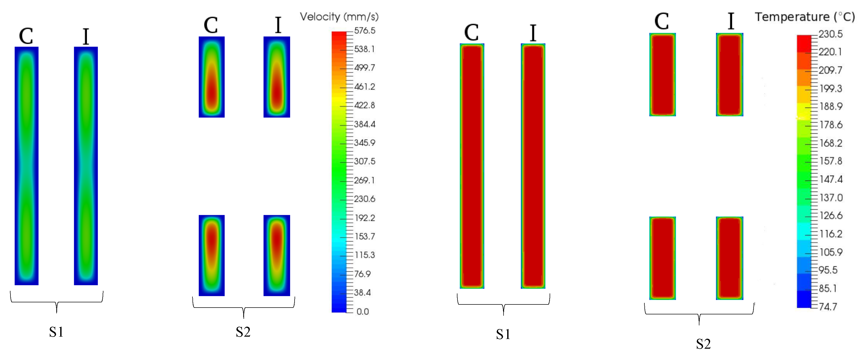
The results obtained using all the meshes considered did not present substantial differences; therefore, only the ones corresponding to the most refined mesh (M3) are presented. Velocity and temperature contours were taken from two cross-sections at different geometry locations (see Figure 4), representative of the initial flow channel region (Slice 1 (S1)) and at the cylindrical insert (Slice 2 (S2)). These results correspond to the switch-over point, i.e., the end of the filling stage. Figure 5 shows the velocity and temperature contours for S1 and S2 and both fluid formulations.

In S1, the location that was close to the cylindrical insert, the melted material at the center of the channel flowed at a lower velocity than the one that was closer to the top and bottom mold walls. This shows that the material flow division, motivated by the insert, already started in S1. In terms of temperature, as expected, the polymer melt at the center of the channel was hotter than the one at the walls (temperature profiles across the channel thickness are shown in Figure 6). Comparing both material formulations, there are no visible differences, both on the velocity and temperature distributions. The results obtained for S2, the location at the middle of the cylindrical insert, show a symmetric velocity profile because of the channel symmetry. As expected, the velocity magnitude increased because the material had a smaller cross-section to flow through. In what concerns to the temperature field, since the cross-section area was smaller, the maximum temperature slightly exceeded 230${}^{°}$C (see also

Table 8. Minimum, average, and maximum temperature values for slices S1 and S2 (see Figure 4), at the switch-over point.

Slice	Formulation	Temperature (${}^{°}$C)			Relative Differences (%)
		Tmin	Tave	Tmax	Tmin	Tave	Tmax
S1	C (ref)	98.0	214.4	230.2	—	—	—
	I	94.4	214.1	230.4	3.7	1.4	0.1
S2	C (ref)	103.3	213.5	230.3	—	—	—
	I	100.0	213.3	230.6	3.2	0.09	0.1

), which is the temperature imposed at the inlet, a direct effect of the viscous dissipation. Moreover, again, the two formulations show no visible differences, for both velocity and temperature distributions.

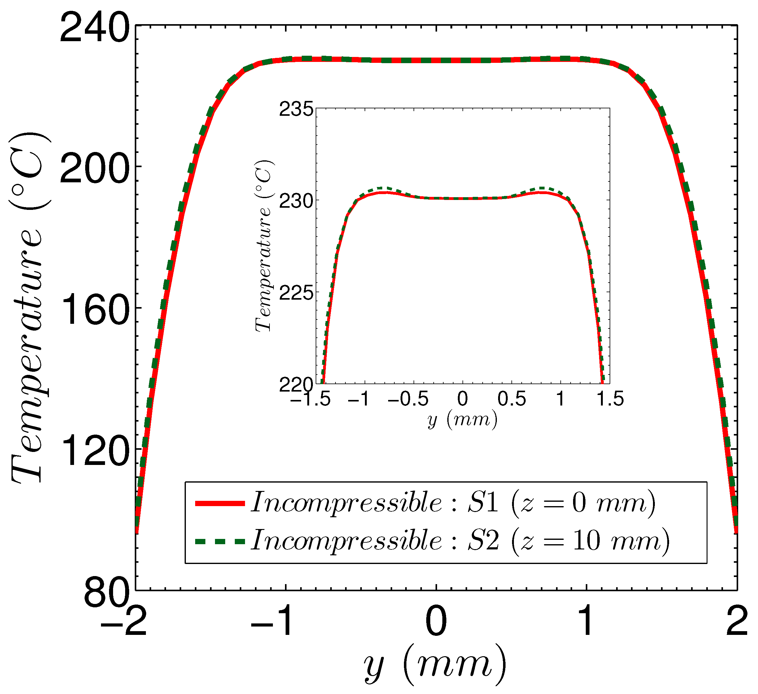
Figure 6 shows the temperature profile across the channel thickness at slices S1 (on $z=0$ mm) and S2 (on $z=10$ mm), for the incompressible fluid formulation. The results obtained with the compressible formulation were similar to the ones presented in Figure 6 and, therefore, are not shown to avoid the clustering of results. Due to the quasi-parabolic velocity profile that is obtained across the thickness, the region of maximum shear-rate, or viscous dissipation, occurs at the wall ($y=\pm$2 mm). However, due to the boundary conditions considered for the temperature field, near the wall, the heat is removed from the polymer melt. As an outcome of this framework, the maximum temperature is obtained at a small distance from the wall. These facts are more evident in the inset provided on Figure 6, which also shows that due to the higher viscous dissipation, motivated by the steeper velocity profile, the maximum temperature was slightly higher in S2 than in S1, in accordance with the maximum temperature values provided in Table 8 (230.4${}^{°}$C in S1 and 230.6${}^{°}$C in S2).

In order to further check the effect of the incompressible formulation, the minimum, average, and maximum values for both fields (temperature and velocity magnitude) were computed for both slices (S1 and S2) at the switch-over point, and the results are presented in Table 8 and

Table 9. Average and maximum velocity magnitude values for slices S1 and S2 (see Figure 4), at the switch-over point.

Slice	Formulation	Velocity (mm/s)		Relative Differences (%)
		Uave	Umax	Uave	Umax
S1	C (ref)	148	342	—	—
	I	149	345	0.7	0.9
S2	C (ref)	233	570	—	—
	I	233	576	0.0	1.0

.

Notice that the minimum value of the velocity field magnitude was not presented in Table 9 because on the mold walls, the no-slip boundary condition was applied for the velocity field. From the results shown in Table 8 and Table 9, we concluded that the differences between the compressible and incompressible formulations in both velocity and temperature fields are negligible, i.e., smaller than 4%.

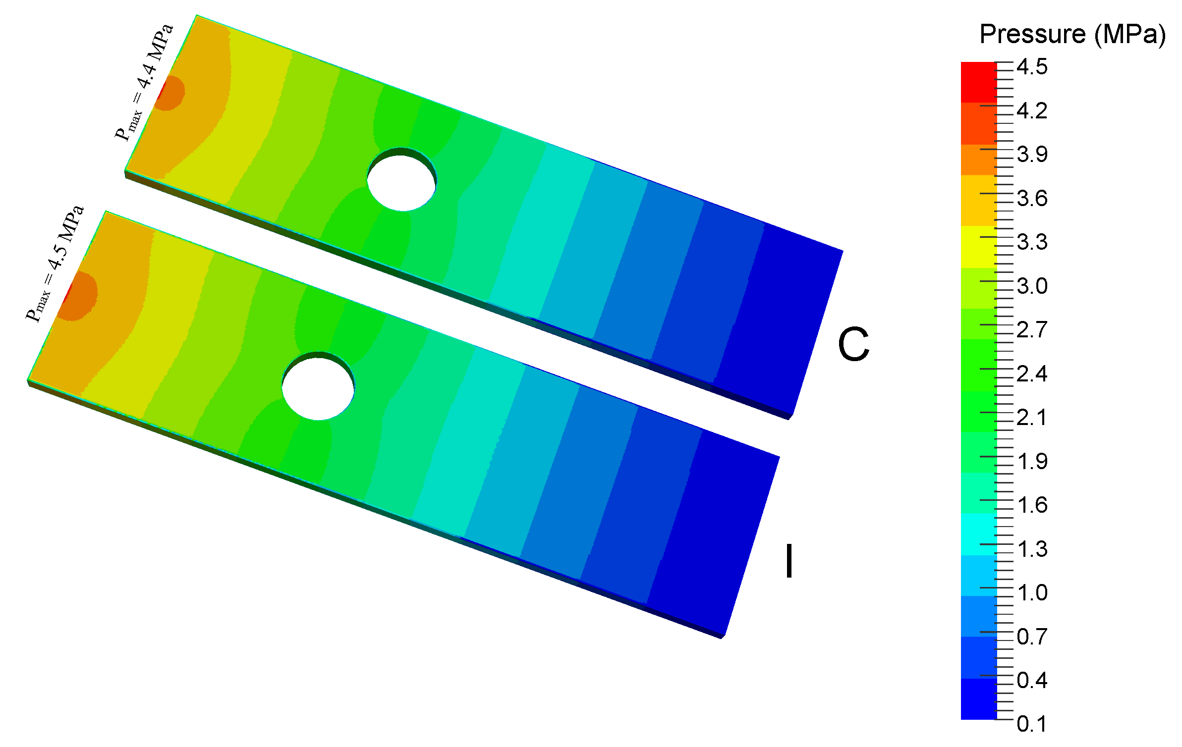
Figure 7 shows the distribution of the pressure field on the mold cavity, computed for both compressible and incompressible formulations, at the switch-over point. These results showed that the maximum pressure required to fill the cavity, predicted by both formulations, was quite similar, with a difference of approximately 0.9%.

From all the results presented, we could conclude that both incompressible and compressible formulations were adequate to be used in the simulation of the filling stage of the IM process, with the former being more advantageous in terms of computational cost. The wall time spent by the incompressible formulation to reach the switch-over point was 39 h, while for the compressible formulation it was 41 h, circa 5% higher. In terms of stability, both formulations, compressible and incompressible, presented similar and good stability during the calculations, due to the use of the PIMPLE (combination of the two acronyms PISO and SIMPLE, while PISO stands for Pressure–Implicit withSplitting of Operators and SIMPLE stands for Semi–Implicit Method for Pressure Linked Equations) algorithm, which allowed obtaining converged solutions in each time-step.

3.3. Case Study 3: Filling of a Tensile Test Specimen

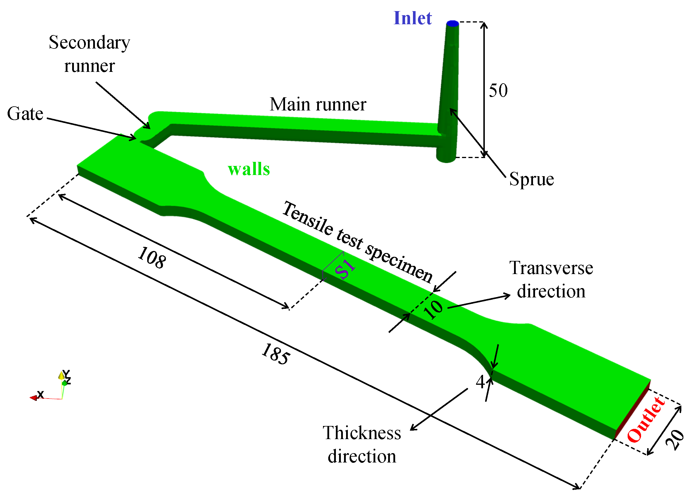
This third case study comprises the simulation of the filling stage of a tensile test specimen. The aim of this case study is to compare the accuracy and performance of $openInjMoldSim$ with the proprietary software Moldex3D^® [11]. This case study geometry, illustrated in Figure 8, is representative of the industrial practice, and corresponds to a specimen used for material mechanical characterization purposes [24,25]. To enlarge the scope of the analysis, the feeding system was included in the simulated geometry. Polymer melt enters the cavity through the inlet boundary located at the top of the sprue. The melted material then flows through the main runner and, subsequently, enters in the secondary runner, which changes the flow melt direction. Before reaching the specimen cavity, the melt flows through a very thin and small channel called the gate [19]. Finally, the melt fills the actual mold cavity, which has a constant thickness of $4\mathrm{mm}$, typical of an injection molded part. The geometry dimensions are given in Figure 8. The boundary patches employed in this case study were similar to the ones of the previous case studies and are also represented in Figure 8. There is an inlet face from which the polymer melt enters and an outlet face from which air exited, while the remaining faces were impermeable walls that only experienced heat flux between the mold and the polymer melt.

The initial and boundary conditions, prescribed in the $OpenFOA{M}^{\circledR }$ [2] library, are presented in Table 1, with an inlet velocity of $U_{in}=1.4$ m/s. In $Moldex3D^{\circledR }$ [11], being proprietary software, many features cannot be defined by the user, as will be shown below for the pressure field. Anyway, the flow rate imposed in $Moldex3D^{\circledR }$ [11] and $OpenFOA{M}^{\circledR }$ [2] was the same and equal to $\mathrm{Q}=15.7$ cm³/s. The temperature boundary conditions were also the same. The pressure field could not be accessed in the proprietary software and, therefore, was the only boundary condition that could not be imposed to be equal in both software.

Since the objective of this study was to make a comparison between the two software, it would be useful to perform the simulations with the same meshes. However, as $Moldex3D^{\circledR }$ [11] only accepts meshes generated in its workbenches, and $OpenFOA{M}^{\circledR }$ [2] could not import those meshes. Consequently, the simulations could not be made exactly in the same meshes. Therefore, the approach employed was to make simulations in meshes with a similar number of cells, until reaching mesh converged results. The same procedure employed in the previous case studies for the mesh sensitivity analysis was also followed here.

Table 10. $openInjMoldSim$ meshes employed in Case Study 3.

Mesh	Number of Cells	Cells Along Transverse Direction	Cells Along Thickness Direction
M1	30,091	8	5
M2	272,149	18	11
M3	2,110,987	37	21

and

Table 11. Moldex3D^® [11] meshes employed in Case Study 3.

Mesh	Number of Cells	Cells Along Transverse Direction	Cells Along Thickness Direction
M1	29,625	8	2
M2	272,409	12	5
M3	2,101,139	26	10
M4	15,304,010	54	21

describe the meshes used in $openInjMoldSim$ and $Moldex3D^{\circledR }$ [11], respectively. The utility $cfMesh$[29] was used to generate the meshes for $openInjMoldSim$; specifically, the Cartesian mesh application was employed to generate the majority of hexahedral cells. The $Moldex3D^{\circledR }$ [11] meshes were created using the program workbench $Moldex3DR16Designer$ [11], applying a boundary layer mesh (BLM). The need to have an additional level of mesh refinement in $Moldex3D^{\circledR }$ [11] will be explained below.

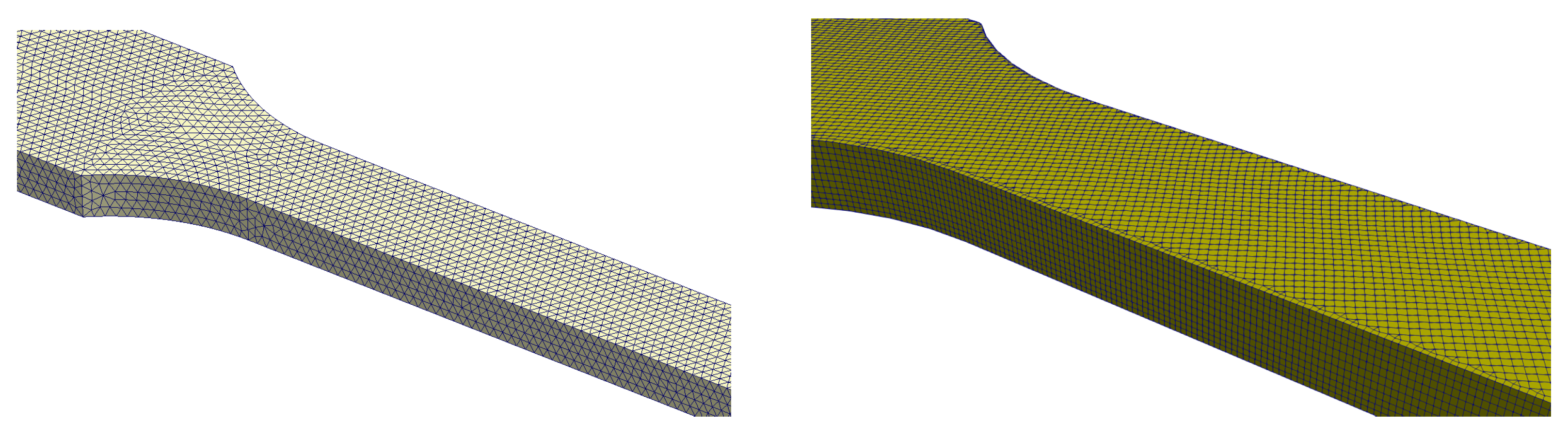
Table 10 and Table 11 show that the number of cells for each mesh refinement level are very close for both software. Additionally, the number of cells for each direction of the tensile test specimen was duplicated in consecutive mesh refinement levels, and consequently, the total number of cells presented a factor of approximately eight. A detailed view of mesh M2 is illustrated in Figure 9 for both software.

The fluids employed in the simulation of the filling of the tensile test specimen were equal to the ones presented in the previous case study, and their properties are given in the introduction of Section 3. Again, the polymer melt was modeled as a generalized Newtonian fluid, while the air was assumed to present a Newtonian behavior.

The aim of the mesh sensitivity analysis was to identify the refinement level required to obtain mesh independent results. To verify the level of refinement needed to ensure the desired accuracy, the Richardson’s extrapolation [30] was applied to the pressure field.

Table 12. Maximum pressure values obtained with the proprietary software $Moldex3D^{\circledR }$ [11] and the open-source software $openInjMoldSim$ at the switch-over point. The Richardson’s extrapolated (RE) values and the relative errors are also presented.

Mesh	$\mathit{Moldex}3{\mathit{D}}^{\mathit{\circledR }}$[11]		$\mathit{openInjMoldSim}$
	Maximum Pressure (MPa)	Error (%)	Maximum Pressure (MPa)	Error (%)
M1	7.18	43.4	7.76	29.6
M2	8.32	34.4	14.07	27.8
M3	9.66	23.8	12.01	9.1
M4	11.61	8.41	-	-
RE	12.68	-	11.01	-

shows the values of the maximum pressure generated in the tensile test specimen cavity, the respective extrapolated value (RE), and the associated errors for both software. The values considered in this analysis were the ones corresponding to the switch-over point.

From Table 12, it is possible to understand the reason for the existence of four levels of mesh refinement in $Moldex3D^{\circledR }$ [11]. For this software, the error for mesh M3 was still very high (>20%); therefore, a fourth mesh was employed, which allowed reaching the same order of accuracy of $openInjMoldSim$. It is important to notice that the maximum values are more difficult to compute, since they tend to have larger errors, due to the fact that they were local values and, therefore, presenting larger sensitivity to numerical errors.

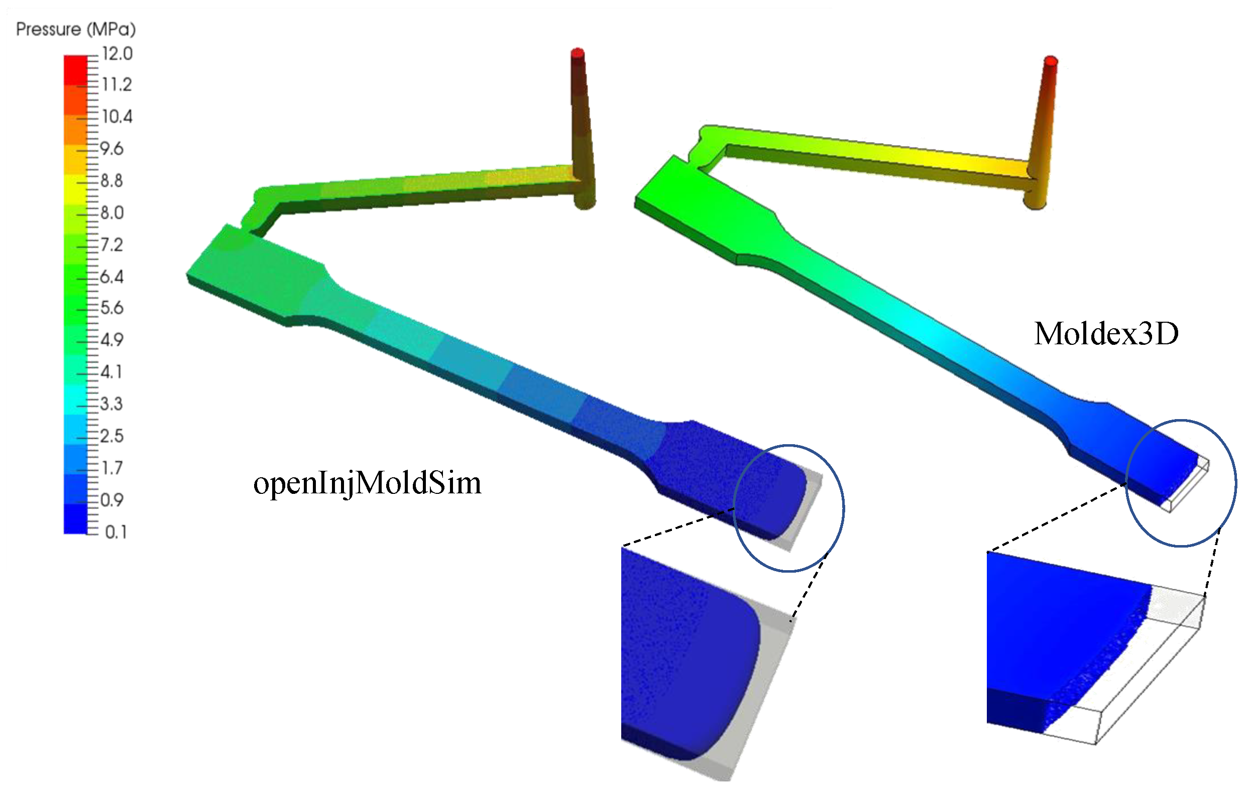
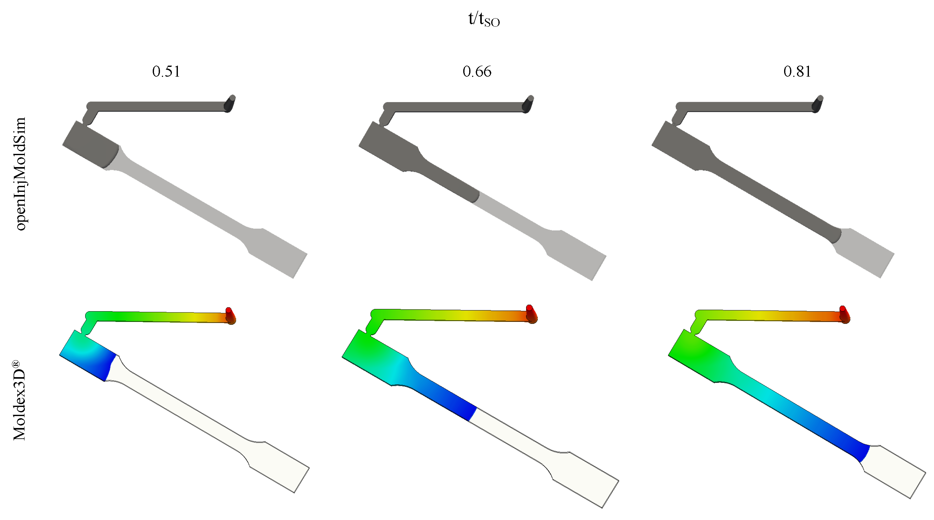
Figure 10 shows the contour of the pressure field distribution in the cavity at the switch-over point. The pressure profiles obtained in both software are qualitatively identical, when using the most refined meshes for both (M4 for $Moldex3D^{\circledR }$ and M3 for $openInjMoldSim$). However, as also shown in Figure 10, the melt flow front predicted by the open-source software seemed more realistic than that of the proprietary counterpart, which present a plug-like surface.

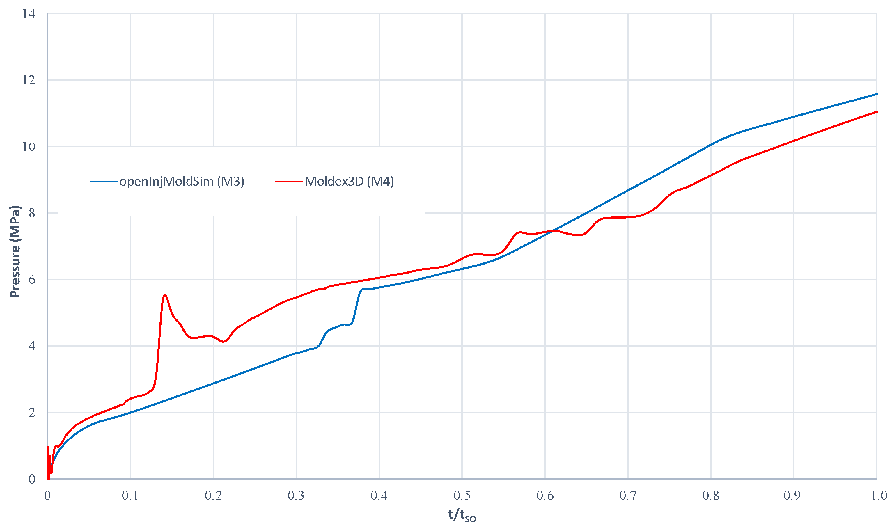
Additionally, as illustrated in Figure 11, the inlet pressure evolution along time was also monitored and compared between both software, using the results obtained with the most refined mesh.

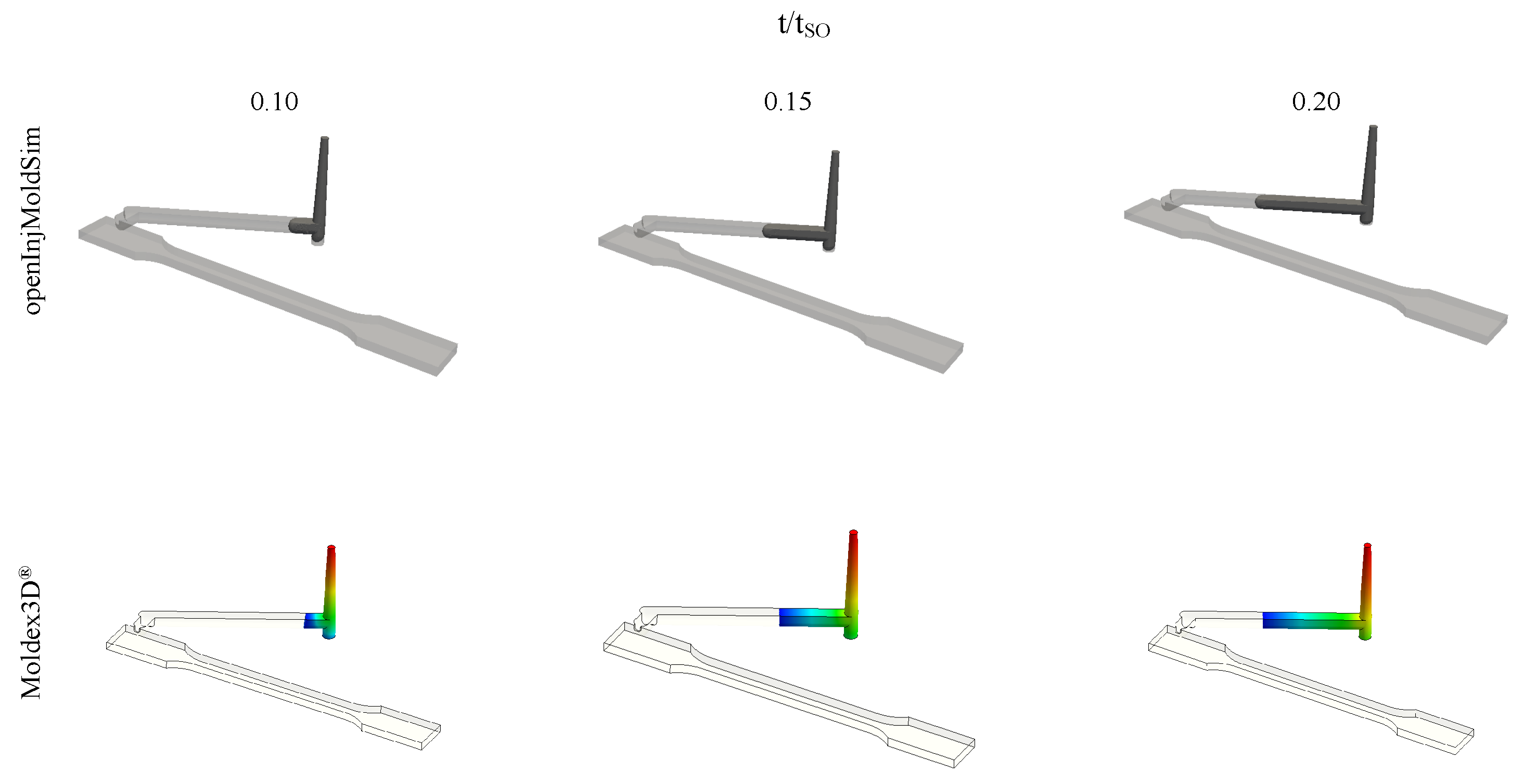
The melt pressure evolution presented some perturbations, which were compared with the progression of the melt flow front. The time intervals where the pressure evolution was perturbed were $0.1<t/t_{SO}<0.2$, $0.3<t/t_{SO}<0.4$, and $0.5<t/t_{SO}<0.8$. The evolution of the melt flow front for the first interval is illustrated in Figure 12. This perturbation in the pressure field was only predicted by $Moldex3D^{\circledR }$ [11], but this behavior seems strange because at $t/t_{SO}=0.1$, the melt flow front was already at the main runner.

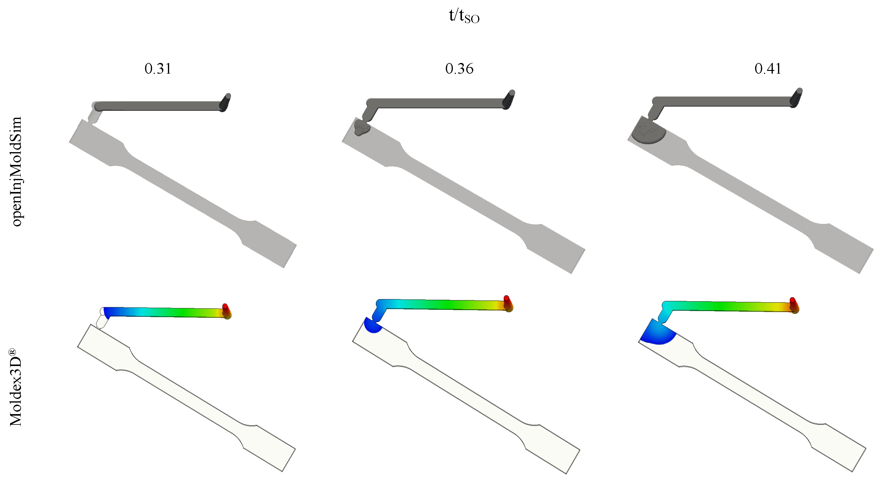
The melt flow front evolution for the second perturbation identified on the inlet pressure evolution is shown in Figure 13, and it coincides with the flow of the melt through the gate. This second perturbation was only predicted by the $openInjMoldSim$ software.

As explained before, the gate was a very small and thin channel; thus, it presented a high resistance to the flow, which justifies the change in the slope on the pressure evolution [19].

The flow front location for the last perturbation observed in the time evolution of the inlet pressure is illustrated in Figure 14. As shown, this interval corresponds to the flow of the melt front through the thinner region of the tensile test specimen. As the cross-section is narrower in that location, a change of the slope in the pressure evolution was expected.

The graph presented in Figure 11 shows that for $openInjMoldSim$, the slope of the curve was higher in the third interval, when compared to the periods before and after it. In $Moldex3D^{\circledR }$ [11] for M4, the pressure evolution curve presents several nonphysical oscillations; however, the pressure is still increasing, as expected.

Finally, a general overview of the accuracy and performance of both software can be obtained from the data presented in

Table 13. General comparison of the accuracy and performance of both $openInjMoldSim$ and $Moldex3D^{\circledR }$ [11].

Software	Mesh	Errors (%)			Number of Cores	Execution Time
		Pmax	Umax	Tmax
Moldex3D® [11]	M1	43.4	14.2	0.7	1	88 s
	M2	34.4	19.6	0.6	1	23 min
	M3	23.8	20.4	0.5	8	3.8 h
	M4	8.41	7.22	0.2	8	24.5 h
openInjMoldSim	M1	29.6	33.2	1.0	1	12.8 h
	M2	27.8	26.7	0.1	8	41 h
	M3	9.1	8.2	0.0	48	98.5 h
					96	59 h
					192	34 h

, where the errors that correspond to the three variables (pressure, velocity, and temperature), as well as the execution time for each level of mesh refinement are given.

From the results shown in Table 13, one can conclude that, in general, $openInjMoldSim$ present better accuracy than $Moldex3D^{\circledR }$ [11], with the exception of the temperature field, where the errors are similar. In order to reach the same accuracy for all fields, $Moldex3D^{\circledR }$ [11] needed at least one more degree of mesh refinement than $openInjMoldSim$. It should be noticed that for the proprietary software, the results did not converge asymptotically with the mesh refinement, which forced to use the Richardson’s extrapolation approach given by Equation (A1), and estimate the apparent order.

In terms of performance, the proprietary software was clearly faster than the open-source for the same level of refinement. $Moldex3D^{\circledR }$ [11] was 523, 107, and 9 times faster than $openInjMoldSim$, respectively for M1, M2, and M3, although they were not computed with the same number of cores. However, when analyzing degrees of mesh refinement for the same accuracy, M3 for $openInjMoldSim$ and M4 for $Moldex3D^{\circledR }$ [11], the proprietary software was only 1.4 times faster than the open-source one; however, the number of cores used was not the same. Notice that, since $Moldex3D^{\circledR }$ [11] is a proprietary software, there is a restricted number of licenses, which did not allow us to solve the problem with more cores. On the other side, since in $OpenFOA{M}^{\circledR }$ [2] the only limitation is the computational resources available, if the number of cores are increased, a similar calculation time could be obtained.

4. Conclusions

A numerical formulation available in the open-source computational library $OpenFOA{M}^{\circledR }$ [2], the $openInjMoldSim$ solver, was assessed in different test cases related to the simulation of the filling stage of the injection molding process.

The verification/validation of the open-source solver was performed with three case studies, where the results obtained with the open-source solver were compared both with analytical solutions, for simpler case studies, and with results obtained with $Moldex3D^{\circledR }$ [11], a proprietary software widely employed in the industry.

The first case study allowed identifying the more appropriate modeling setup and to understand some details of the numerical algorithm developed to describe the injection molding process, by considering the simplified Newtonian constitutive model. The results obtained with this first case study allowed us to conclude that the artificial interface compression term, presented in the volume of fluid formulation, provided better results for coarse and medium meshes, but in refined meshes, it affected the mass conservation negatively. Furthermore, the open-source solver predictions presented a good agreement with the analytical reference solutions. Finally, the compressible formulation did not present substantial differences in relation to the incompressible one.

In the second case study, two formulations for the equation of state (compressible and incompressible) based on the modified Tait model were used. This study allowed verifying that in the presence of incompressible formulations, the performance of the numerical algorithm was improved without a significant loss of accuracy. This observation further indicated that incompressible formulations were a good approximation for the filling stage of the injection molding process and may be a way of increasing the overall calculation efficiency.

In the third case study, the results obtained with $openInjMoldSim$ and $Moldex3D^{\circledR }$ [11] were compared. The open-source software presented results that practically converged, i.e., with relative errors below 10% within three levels of mesh refinement. Additionally, its accuracy was better than the proprietary software for each level of mesh refinement. In order to reach the same accuracy obtained with $openInjMoldSim$, $Moldex3D^{\circledR }$ [11] required an additional level of mesh refinement. Moreover, the latter did not present asymptotic convergence of the errors with the mesh refinement. Furthermore, a few nonphysical results were obtained with the proprietary software, both in terms of the flow front shape, and in the evolution of inlet pressure, in which, for instance, the flow of the melt front through the gate could not be identified. The open-source software did not present similar limitations.

All these results led to the conclusion that the $openInjMoldSim$ solver presented a better accuracy than $Moldex3D^{\circledR }$ [11]. In terms of performance, the scenario was reversed, with $Moldex3D^{\circledR }$ [11] being clearly faster than the $openInjMoldSim$ solver. However, one of the main limitations of the proprietary software is the number of licenses available. Therefore, if there were enough computational resources available, open-source software could match the calculation speed of the proprietary one.

In summary, the results presented here showed that the injection molding code, developed using an open-source framework, could be used to model the filling stage of injection molding processes accurately. However, additional studies should be made to improve the calculation performance.

References

1. Kennedy, P.; Zheng, R. Flow Analysis of Injection Molds, 2nd ed.; Hanser: Munich, Germany, 2001. [Google Scholar]
2. OpenFOAM. The Open Source CFD Toolbox. Available online: https://www.openfoam.com/ (accessed on 27 May 2020).
3. Habla, F.; Fernandes, C.; Maier, M.; Densky, L.; Ferrás, L.L.; Rajkumar, A.; Carneiro, O.S.; Hinrichsen, O.; Nóbrega, J.M. Development and validation of a model for the temperature distribution in the extrusion calibration stage. Appl. Therm. Eng. 2016, 100, 538–552. [Google Scholar] [CrossRef]
4. Rajkumar, A.; Ferrás, L.L.; Fernandes, C.; Carneiro, O.S.; Nóbrega, J.M. Guidelines for balancing the flow in extrusion dies: The influence of the material rheology. J. Polym. Eng. 2017, 38, 197–211. [Google Scholar] [CrossRef]
5. Araújo, B.J.; Teixeira, J.C.F.; Cunha, A.M.; Groth, C.P.T. Parallel three-dimensional simulation of injection molding process. Int. J. Numer. Methods Fluids 2009, 59, 801–815. [Google Scholar] [CrossRef]
6. Nagy, J.; Steinbichler, G. Fluid Dynamic and Thermal Modeling of the Injection Molding Process in OpenFOAM. In OpenFOAM Selected Papers of the 11th Workshop; Nóbrega, J.M., Jasak, H., Eds.; Springer: Cham, Switzerland, 2019. [Google Scholar]
7. Magalhães, A. OpenFOAM Simulation of the Injection Moulding Filling Stage. Master’s Thesis, Integrated Master in Polymer Engineering, University of Minho, Braga, Portugal, September 2016. Available online: http://repositorium.sdum.uminho.pt/handle/1822/65291 (accessed on 27 May 2020).
8. Mole, N.; Krebelj, K.; Stǒk, B. Injection molding simulation with solid semi-crystalline polymer mechanical behavior for ejection analysis. Int. J. Adv. Manuf. Technol. 2017, 93, 4111–4124. [Google Scholar] [CrossRef] [Green Version]
9. Krebelj, K.; Turk, J. An Open–Source Injection Molding Simulation. A Solver for OpenFOAM. Available online: https://github.com/krebeljk/openInjMoldSim (accessed on 10 September 2019).
10. Fontaínhas, A. Injection Moulding Simulation Using OpenFOAM. Master’s Thesis, Integrated Master in Polymer Engineering, University of Minho, Braga, Portugal, 2019. Available online: https://www.researchgate.net/publication/341448307_Injection_moulding_simulation_using_OpenFOAM (accessed on 27 May 2020).
11. Moldex 3D. Plastic Injection Molding Simulation Software. Available online: https://www.moldex3d.com/ (accessed on 27 May 2020).
12. Pichelin, E.; Coupez, T. Finite element solution of the 3D mold filling problem for viscous incompressible fluid. Comput. Methods Appl. Mech. Eng. 1998, 163, 359–371. [Google Scholar] [CrossRef]
13. Berberović, E.; van Hinsberg, N.P.; Jakirlić, S.; Roisman, I.V.; Tropea, C. Drop impact onto a liquid layer of finite thickness: Dynamics of the cavity evolution. Phys. Rev. E 2009, 79, 036306. [Google Scholar] [CrossRef] [PubMed]
14. Hirt, C.W.; Nichols, B.D. Volume of fluid (VOF) method for the dynamics of free boundaries. J. Comput. Phys. 1981, 39, 201–225. [Google Scholar] [CrossRef]
15. Haider, J. Numerical Modelling of Evaporation and Condensation Phenomena. Master’s Thesis, Universität of Stuttgart, Stuttgart, Germany, 2013. [Google Scholar]
16. Rusche, H. Computational Fluid Dynamics of Dispersed Two-Phase Flows at High Phase Fractions. Ph.D. Thesis, Department of Mechanical Engineering from the Imperial College of Science, Technology and Medicine, University of London, London, UK, 2002. [Google Scholar]
17. Chiang, H.H.; Hieber, C.A.; Wang, K.K. A unified simulation of the filling and postfilling stages in injection molding. Part I: Formulation. Polym. Eng. Sci. 1991, 31, 116–124. [Google Scholar] [CrossRef]
18. Williams, M.L.; Landel, R.F.; Ferry, J.D. The Temperature Dependence of Relaxation Mechanisms in Amorphous Polymers and Other Glass-forming Liquids. J. Am. Chem. Soc. 1955, 77, 3701–3707. [Google Scholar] [CrossRef]
19. Zhou, H. Computer Modelling for Injection Molding; John Wiley & Sons, Inc.: Hoboken, NJ, USA, 2013. [Google Scholar]
20. Rees, H. Understanding Injection Mold Design; Hanser Publications: Cincinnati, OH, USA, 2001. [Google Scholar]
21. Tait, P.G. Physics and Chemistry of the Voyage of H.M.S. Challenger; HMSO: London, UK, 1888; Volume 2, pp. 941–951. [Google Scholar]
22. Ferziger, J.H.; Peric, M. Computational Methods for Fluid Dynamics; Springer: Cham, Switzerland, 2001. [Google Scholar]
23. Jasak, H. Error Analysis and Estimation for the finite Volume Method with Application to Fluid Flows. Ph.D. Thesis, Imperial College, University of London, London, UK, 1996. [Google Scholar]
24. Liang, J.; Luo, W.; Huang, Z.; Zhou, H.; Zhang, Y.; Zhang, Y.; Fu, Y. A robust finite volume method for three-dimensional filling simulation of plastic injection molding. Eng. Comput. 2017, 34, 814–831. [Google Scholar] [CrossRef]
25. Kim, K.H.; Isayev, A.I.; Kwon, K.; van Sweden, C. Modelling and experimental study of birefringence in injection molding of semicrystalline polymers. Elsevier Polym. 2005, 46, 4183–4203. [Google Scholar] [CrossRef]
26. Rosato, D.V.; Rosato, M.G. Injection Molding Handbook; Springer: Cham, Switzerland, 2000. [Google Scholar]
27. Celik, I.; Ghia, U.; Freitas, C.J.; Coleman, H.; Raad, P.E. Procedure for Estimation and Reporting of Uncertainty Due to Discretization in CFD Applications. J. Fluids Eng. 2008, 130, 1–4. [Google Scholar] [CrossRef] [Green Version]
28. Oberkampf, W.L.; Trucano, T.G.; Hirsch, C. Verification, validation, and predictive capability in computational engineering and physics. Appl. Mech. Rev. 2004, 57, 345–384. [Google Scholar] [CrossRef] [Green Version]
29. Juretic, F. A Library for Automatic Mesh Generation. Available online: https://cfmesh.com/cfmesh/ (accessed on 27 May 2020).
30. Richardson, L.F. On the Approximate Arithmetical Solution by Finite Differences of Physical Problems Involving Differential Equations, With an Application to the Stresses in a Masonary Dam. Philos. Trans. R. Soc. Lond. 1910, 210, 307–357. [Google Scholar] [CrossRef] [Green Version]
31. Celik, I.; Karatekin, O. Numerical experiments on application of Richardson extrapolation with non-uniform grids. J. Fluids Eng. 1997, 119, 584–590. [Google Scholar] [CrossRef]
32. Fernandes, C.; Faroughi, S.A.; Carneiro, O.S.; Miguel Nóbrega, J.; McKinley, G.H. Fully-resolved simulations of particle-laden viscoelastic fluids using an immersed boundary method. J. Non Newton. Fluid Mech. 2019, 266, 80–94. [Google Scholar] [CrossRef] [Green Version]
Figure 1. Variation of the viscosity with shear-rate and temperature for the GPPS Styron 678.
Fluids 05 00084 g001
Figure 2. Variation of the polymer specific volume with temperature and pressure fields for the GPPS Styron 678.
Fluids 05 00084 g002
Figure 3. Geometry of the cylindrical cavity for Case Study 1 (dimensions in mm).
Fluids 05 00084 g003
Figure 4. Geometry and boundary patches for Case Study 2 (dimensions in mm). S1 and S2 denotes Slice 1 and Slice 2, respectively.
Fluids 05 00084 g004
Figure 5. Velocity magnitude (left) and temperature (right) contours on slices S1 and S2 for Case Study 2. C, compressible formulation; I, incompressible formulation.
Fluids 05 00084 g005
Figure 6. Temperature profiles across the channel thickness at slices S1 and S2, using the incompressible formulation, for Case Study 2.
Fluids 05 00084 g006
Figure 7. Distribution of the pressure field on the mold cavity, for the two formulations, compressible (C) and incompressible (I), at the switch-over point.
Fluids 05 00084 g007
Figure 8. Geometry and boundary walls for Case Study 3 (dimensions in mm).
Fluids 05 00084 g008
Figure 9. Mesh M2 for M o l d e x 3 D ® [11] (left) and o p e n I n j M o l d S i m (right).
Fluids 05 00084 g009
Figure 10. Pressure distribution at the switch-over point and melt flow front shape predicted by the most refined mesh of both software.
Fluids 05 00084 g010
Figure 11. Time evolution of the inlet pressure obtained with the most refined mesh for both o p e n I n j M o l d S i m and M o l d e x 3 D ® [11] software.
Fluids 05 00084 g011
Figure 12. Melt front location for t / t S O = 0.1 , 0.15 , and 0.2 predicted by both o p e n I n j M o l d S i m and M o l d e x 3 D ® [11].
Fluids 05 00084 g012
Figure 13. Melt front location for t / t S O = 0.31 , 0.36 , and 0.41 predicted by both o p e n I n j M o l d S i m and M o l d e x 3 D ® [11].
Fluids 05 00084 g013
Figure 14. Melt front location for t / t S O = 0.51 , 0.66 , and 0.81 predicted by both o p e n I n j M o l d S i m and M o l d e x 3 D ® [11].
Fluids 05 00084 g014