Article

A Viscous, Two-Layer Western Boundary Current Structure Function

by
Charles W. McMahon
1,
Joseph J. Kuehl
1,* and
Vitalii A. Sheremet
2
1
Department of Mechanical Engineering, University of Delaware, Newark, DE 19716, USA
2
Graduate School of Oceanography, University of Rhode Island, Narragansett, RI 02882, USA
*
Author to whom correspondence should be addressed.
Fluids 2020, 5(2), 63; https://doi.org/10.3390/fluids5020063
Submission received: 5 March 2020 / Revised: 22 April 2020 / Accepted: 23 April 2020 / Published: 28 April 2020
(This article belongs to the Collection Geophysical Fluid Dynamics)

Abstract

:
The classic oceanographic problem of a 1.5-layer western boundary current evolving along a straight wall is considered. Here, building upon the previous work of Charney, Huang and Kamenkovich, we have derived, solved and validated a new numerical formulation for accounting for viscous effects in such systems. The numerical formulation is validated against rotating table experimental results.

1. Introduction

The objective of this manuscript is to gain insight into the fundamental physics of oceanic western boundary currents and their layered laboratory models. Specifically, we will explore the asymmetry observed in laboratory results between the poleward and equatorward flowing boundary currents corresponding to the subtropical and subpolar gyre regions. The theoretical analysis of western boundary currents (WBCs) originated with the seminal works of Prandtl [1], Blasius [2], Stommel [3], Munk [4], and Schlichting [5] developing the boundary layer approach. For the ocean, the boundary layer approach is justified by the relative narrowness of the current systems such as the Gulf Stream and Kuroshio (≈100 km) compared to the scale of the subtropical gyre circulation (≈2000–10,000 km). The single fixed depth layer, depth-averaged, or barotropic case is well established with the fundamental balances resulting in the familiar Stommel, Munk, and inertial lateral boundary layers (e.g., Pedlosky [6]). A simultaneous combination of lateral friction and inertia was considered in a series of works by Il’in and Kamenkovich [7,8]. Kamenkovich [9] considered this as well and obtained an explicit analytic solution using a functional relationship for a special class of boundary current transport with parabolic dependence, 4 y ( 1 y ) , on latitude 0 < y < 1 . In contrast, a more common sinusoidal dependence sin ( π y ) was used in later studies by Ierley and Ruehr [10] and Mallier [11] using semi-analytic/numerical methods.
The effect of a varying layer thickness (1.5-layer model and associated nonlinearity) was considered by Charney [12] assuming a purely inviscid inertial western boundary current. Charney’s approach was to derive relationships between the Bernoulli function, potential vorticity, and stream function which are specified outside the boundary layer (in the ocean interior). These far-field conditions could then be functionally mapped into the boundary region to obtain an inviscid approximation to the inertial western boundary current structure. Charney’s method was extended by Huang [13] in a 2.5-layer inviscid model (consisting of two moving fluid layers with the third layer being much deeper and stagnant).
A 1.5-layer solution will be considered here but we seek to remove the inviscid restriction, which will extend the earlier analysis of Kuehl and Sheremet [14,15,16]. It should be noted that this work considers a vertical wall with no sloping topography. Thus, the bottom pressure torque concept of Hughes [17] and Hughes and Cuevas [18]) is not active. Other researchers, such as Pierini et al. [19,20] on a 5 m rotating platform, often used the vertical wall approximation, thus considering large scale motions. The role of sloping bathymetry on the boundary current structure was studied by Salmon [21] using a 2-layer approach. Nonetheless, the observational study of Beal and Bryden [22] suggests that a vertical wall, layered western boundary current formulation is relevant to the Agulhas current (around 32 S).
This manuscript is organized as follows. In 
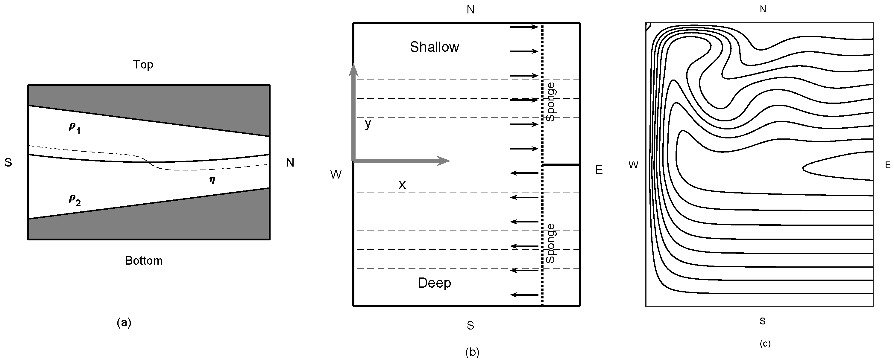
Section 2, we discuss the problem formulation for a 1.5-layer western boundary current in the context of a rotating table laboratory experiment. These experiments were carried out in Kuehl and Sheremet [16] and resulted in WBCs with north–south flowing asymmetry, which could not be described with simple theory. In Section 3, the mathematical formulation of the problem is described. We derive the relevant vorticity equation which describes the structure function of an upper-layer intensified and accelerating western boundary current, and solve it numerically. The numerical boundary current profiles are then compared with experimental measurements. Section 5 is a brief summary of the results.

2. Problem Formulation

2.1. Model

We formulate the problem of layered oceanographic flow in the context of a two-layer rotating table experiment. Consider a square rotating tank (with side length of 2 L = 0.763 m) in which two fluid layers of different densities ( ρ 1 and ρ 2 ) are contained between a sloping rigid-lid and sloping bottom (Figure 1, panel a). We put the origin of the cartesian coordinate system ( x , y ) at the center of the tank and the center of the platform rotation. The upper layer depth can be decomposed as h 1 = H 1 ( x , y ) + η ( x , y ) , where H 1 = H 01 Ω 2 r 2 / ( 2 g ) S y is the mean layer depth in a solid body rotation, r = x 2 + y 2 is the distance from the center, g = 9.803 m/s 2 is the acceleration due to gravity, and η is the interface displacement (down) relative to the no motion state. Similarly, the lower layer depth is h 2 = H 2 ( x , y ) η ( x , y ) , where H 2 = H 02 + Ω 2 r 2 / ( 2 g ) S y . The platform rotation with rate Ω (typically 1 rad/s) gives rise to the Coriolis effect, f = 2 Ω is the Coriolis parameter and, in combination with the top and bottom lid slopes of S = 0.1 , induces a topographic β -effect in each layer. This models the planetary β -effect with x being analogous to eastward and y northward directions. In the nonrotating state the layer thicknesses were H 01 N R = 15 cm and H 02 N R = 5 cm at the center with the total thickness 20 cm. As the interface assumes the shape of a paroboloid in a solid body rotation, the steady thickness of the upper layer at the center slightly increases to 15.5 cm according to H 01 = H 01 N R + Ω 2 L 2 / ( 3 g ) , due to conservation of the layer volume as the mass redistributes.
Sketched in Figure 1 (panel b) is the experimental setup (also used by Kuehl and Sheremet [16]), in which a broad Sverdrup interior flow is driven by pumping fluid through sponges at the eastern boundary. Such pumping produces inflow (outflow) in the upper layer only with uniform velocity U i n ( U o u t ) due to the pressure drop across the sponge. The interior flow follows isobaths (indicated by dashed lines) and impinges onto the western boundary x = 0 where a boundary current is formed. Figure 1 (panel c) shows a typical numerical solution illustrating the flow pattern corresponding to the oceanic subtropical gyre with a northward flowing western boundary current. The opposite sense of pumping will produce a southward flowing boundary current corresponding to the oceanic subpolar gyre.

2.2. Procedure

The procedure to model a boundary current in the laboratory begins with filling two open storage tanks with warm water and allowing them to cool to room temperature (≈ 20 C). Warm water contains less dissolved oxygen that would otherwise increase the formation of bubbles on the rigid lid of the experimental tank, which negatively effects the accuracy of flow measurements. Salt is mixed into one container before it equilibrates with room temperature, to set the density of the water that will fill the lower layer. The experimental tank is then filled with the fresh water and seeding particles are introduced. The table and tank are set to rotate at constant rate Ω . The fluid is allowed enough time to reach solid-body rotation with no flow. The lower-layer is then slowly filled from the bottom of the tank with the denser salt water while the table is rotating. The lower-layer is filled until the interface between layers reaches the top of a parabolic insert which separates the lower-layer from the forcing region sponges. In Figure 1 (panel a), the area of the parabolic insert is labeled by ρ 2 and is bounded by solid lines, matching the lower layer thickness. It is a divider that allows the forcing sponges to only initiate flow in the upper layer. The flow domain between the sloping bottom and sloping rigid lid is now filled completely with two layers, with a typical density difference between layers of Δ ρ = 7.510 3 g cm 3 , providing a robust interface. The two fluid layers are allowed to reach solid body rotation. Forcing of the upper layer is then initiated by pumping water from one forcing sponge basin to the other at a specified flow rate (setting the transport of the boundary current). This causes a boundary current to form in the upper layer along the wall at x = 0 , with an unforced lower layer. Transient behavior is allowed subside and the steady-state boundary current is imaged with particle image velocimetry (PIV).

2.3. Flow Visualization

The PIV system, which measures velocity vectors of the boundary current, is described as the following. The passive seeding particles in the upper layer are illuminated with a horizontal laser light sheet and imaged with a 1376 × 1040 pixel CCD camera. The particles are glass spheres of 10-micron diameter. The light sheet is created by a 50 mJ Nd-YAG laser emits a 5 ns pulse of light through a diverging lens. The laser and camera are synchronized such that each laser pulse corresponds to one image and the time difference (90,000 μ s) between two consecutive pulses (images) is known. The system has a maximum frequency of 4 Hz, so four two-image pairs may be obtained every second. These settings are adequate for laboratory boundary current velocities of a few cm s 1 . Once a series of images are recorded, software correlates the particle movements between two consecutive images in small windows ( 32 × 32 pixels), yielding a two dimensional array of velocity vectors. The laser and camera were attached to a superstructure, which was mounted around the tank on the rotating table. The laser was mounted to the west of the tank and illuminated the boundary current in a horizontal plane, set in the center of the layer of interest. The camera was suspended directly above the flow, as in the view of the middle and right panels of Figure 1. The resulting boundary current velocity measurements will be used later to validate the numerical solution in this investigation.

3. Mathematical Formulation

In this work, we will consider a 1.5-layer approximation: the flow is concentrated in the upper layer, the lower-layer flow is assumed to be negligible because there is no pumping and the geostrophic contours (lines of f / h 2 = c o n s t ) are blocked. We start with the shallow water equations assuming that the velocity field ( u , v ) is depth independent. This is primarily a consequence of the rapid rotation of the experimental platform which results in a small Rossby number R o = U 0 / f L , where U 0 is a typical velocity scale. The momentum equations and continuity equation for the single active fluid layer are:
u t ( f + ω ) v + ( p + e ) x = k u + ν 2 u v t + ( f + ω ) u + ( p + e ) y = k v + ν 2 v h t + ( h u ) x + ( h v ) y = 0 .
The layer identifying subscripts have been dropped as Equationreds (1) are valid for either layer. Details can be found in Pedlosky [6] or, in particular, the Cushman–Roisin [23] chapter on layered systems. However, unlike the traditional geostrophic approximation, we admit the finite depth layer changes. More explicitly, Kuehl and Sheremet [16] provides the coupled two-layer system set of equations. Equations (1) for the upper active layer are the result of taking the 1.5-layer limit.
In Equations (1): u , v are the cross-shore and alongshore velocities, respectively, (in the context of the western boundary current), h is the depth of the fluid layer, e = ( u 2 + v 2 ) / 2 is kinetic energy per unit mass, ω = v x u y is the vorticity, ν is the lateral viscosity, f is the Coriolis parameter, and p is the pressure anomaly relative to no motion, divided by the fluid density ( ρ ). As this work considers layered systems, p can also be interpreted as the Montgomery Potential. Either way, p = g η is obtained, where g = ( Δ ρ / ρ 1 ) g is the reduced gravity, and Δ ρ = ρ 2 ρ 1 . The Rayleigh drag terms ( k u , k v ) are assumed to be uniformly distributed over the fluid layer. Our intention is to consider steady state solutions, but we included the temporal derivative terms to remind the reader of the broader context.
Taking the curl of the momentum equations, defining the transport function ( ψ ) through h u = ψ y and h v = ψ x to satisfy the steady continuity equation and introducing the potential vorticity q = ( f + ω ) / h gives us the steady state vorticity advection–diffusion equation:
J ( ψ , q ) = k ω + ν 2 ω ,
where J is the Jacobian operator. The Rayleigh drag originates from the Ekman flux divergence due to the top/bottom and interfacial friction effects, their combined result can be expressed as k = 3 4 f ( h E / h ) , where h E = 2 ν / f is the Ekman layer depth.
In order to solve the problem, we also need a relationship between the transport function ψ and the pressure or the layer thickness anomaly η . In the classical quasigeostrophic approximation (Pedlosky [6]) it is assumed that η is proportinal to ψ which is valid only for small changes of the layer thickness. We do not use this restriction. Instead, we will use a boundary layer approximation and a semi-geostrophic balance: the geostrophic balance only perpendicular to the boundary, while along the bondary the nonlinear ageostrophic accelerations are retained in the potential vorticity advection-diffusion Equation (2). In the western boundary current, the x-scales of motion are much smaller than y-scales, therefore the cross-flow momentum equation is simplified to a geostrophic balance
f ψ x + g h η x = 0 .
Thus we can integrate along x in order to express the layer thickness h = H + η
h ( x , y ) = h B 2 ( y ) + 2 f g ( ψ ( x , y ) Ψ B ( y ) ) ,
where h B ( y ) and Ψ B ( y ) are the meridional distributions of layer thickness and transport function outside of the western boundary current. Since we are focused on the western boundary current region, without loss of generality, we can assume that H is independent of x, H ( y ) = H 0 Ω 2 y 2 / ( 2 g ) S y , where H 0 = H 01 the upper layer value. The distributions h B ( y ) and Ψ B ( y ) are essentially the same as at the eastern boundary, are established at the sponges by pumping fluid, and are in a geostrophic zonal flow balance. For example, for the inflow half L < y < 0 :
f U i n = g η B y ( y ) ( H ( y ) + η B ( y ) ) U i n = Ψ B y ( y ) .
Similar equtions hold for the outflow half 0 < y < L . The total volume inflow Q = Ψ B ( 0 ) Ψ B ( L ) is specified by pumping and must be the same as the outflow Q = Ψ B ( 0 ) Ψ B ( L ) . We also need to specify that the anomaly η averaged over the whole basin is zero or specify a reference value, for example, η B ( 0 ) = 0 . In our case, both of these conditions are very close. Thus, explicit expressions for η B are
η B ( y ) = f g U o u t y , y > 0 η B ( y ) = f g U i n y , y < 0
and then explicit expression for Ψ B ( y ) can be calculated from (5). The uniform inflow U i n and outflow U o u t velocities are determined from the quadratic Equation (5), but are very close to the linear estimates U i n = Q / ( L H 0 ) and U o u t = Q / ( L H 0 ) .

4. Solution

In order to solve numerically, the nonlinear steady flow problem is cast into a nondimensional form by scaling: x , y by L; h, H and η by H 0 ; u and v by U 0 = Q / ( H 0 L ) ; ω by U 0 / L ; ψ by Q; q by β L / H 0 with β = f S / H 0 being the topographic β -effect. In nondimensional form the problem reads as follows
J ( ψ , q ) + λ S 1 h ω λ M 3 2 ω = 0 ( 1 h ψ ) ω = 0 ,
where q = ( 1 / β ^ + λ I 2 ω ) / h , h = 1 B y 2 β ^ y + η . The nondimensional parameter β ^ = β L / f = S L / H 0 is the relative meridional variation of depth over the basin due to the sloping top lid; and B = f 2 L 2 / ( 8 g H 0 ) is the relative effect of the paraboloidal shape of the fluid interface in a solid body rotation. The domain is 0 < x < x B , x B = 1 / 2 , 1 < y < 1 . The kinematic conditions for solving the elliptic equation are ψ = 0 along all boundaries, except at the eastern boundary x = x B where inflow/outflow is prescribed ψ = Ψ B ( y ) , with Ψ B varying between 0 and 1. The dynamical conditions are no-slip: v = 0 at the western x = 0 and eastern x = x B boundaries and no-stress ω = 0 at the southern y = 1 and northern y = 1 boundaries. The arising parameters λ I = U 0 β L , λ S = k 0 β L with k 0 = 3 4 f ( h E / H 0 ) and λ M = ν β L 1 3 are the nondimensional inertial, Stommel, and Munk boundary layer thicknesses as in the standard quasigeostrophic theory. Lastly, a nondimensional parameter σ = f L U 0 / ( g H 0 ) = R o L 2 / L D 2 appears in the relationship between the flow function and the interface displacement
h η x = σ ψ x h ( x , y ) = h B 2 ( y ) + 2 σ ( ψ ( x , y ) Ψ B ( y ) ) ,
where L D = g H 0 / f is the deformation radius. The expression under the square root may become negative when σ is finite. In this case, the layer thickness may vanish and the equations will break down.
The numerical problem is solved using standard finite differences on a rectangular grid dividing the domain into N x × N y cells. The parameters λ S and λ M represent the dissipative effects, while λ I characterizes the nonlinearity, the strength of pumping. For small boundary layer Reynolds numbers R = ( λ I / λ M ) 3 simple explicit iterations with treating the nonlinear terms as perturbations work well, but for the moderate R the iterations fail to converge. In this case Newton’s method has be to employed for finding steady solutions. We consider a state vector X = ( ω , ψ ) consisting of values at all grid nodes including the boundaries, the size of this vector is M = ( N x + 1 ) ( N y + 1 ) 2 . Substituting an initial guess X 0 into (7) results in the vector of residuals F ( X 0 ) at each grid node of the same size M. In order to find X 1 that brings residual closer to vanishing F ( X ) = 0 , we need to calculate the Jacobian matrix J F [ X 0 ] (of size M × M which depends on X 0 ) of all first-order partial derivatives of F with respect to X and then solve the linear sytem
J F [ X 0 ] ( X 1 X 0 ) = F ( X 0 )
The iterations then continue until the residual completely vanishes. The elements of the Jacobian matrix can be calculated analytically by considering the variational problem corresponding to (7).
J ( δ ψ , q ) + J ( ψ , δ q ) + λ S 1 h δ ω λ M 3 2 δ ω = 0 ( 1 h δ ψ ) δ ω = 0 ,
where δ q = λ I 2 δ ω / h q δ η / h , where δ η = σ δ ψ / h according to (8). The variations of the boundary conditions are trivial. It should be noted that the elements of the Jacobian matrix do not have to be calculated exactly. We may ignore the variation of h in the bottom drag term and in the elliptic equation. As long as the iterations converge and the residual F ( X ) vanishes, we get an exact solution to the original problem (7). Finite difference approximations result in a sparse banded type of J F , and the grids of size upto 1000 × 1000 can be solved on a computer with 24 GiB of operational memory.

Numerical Experimental Comparison

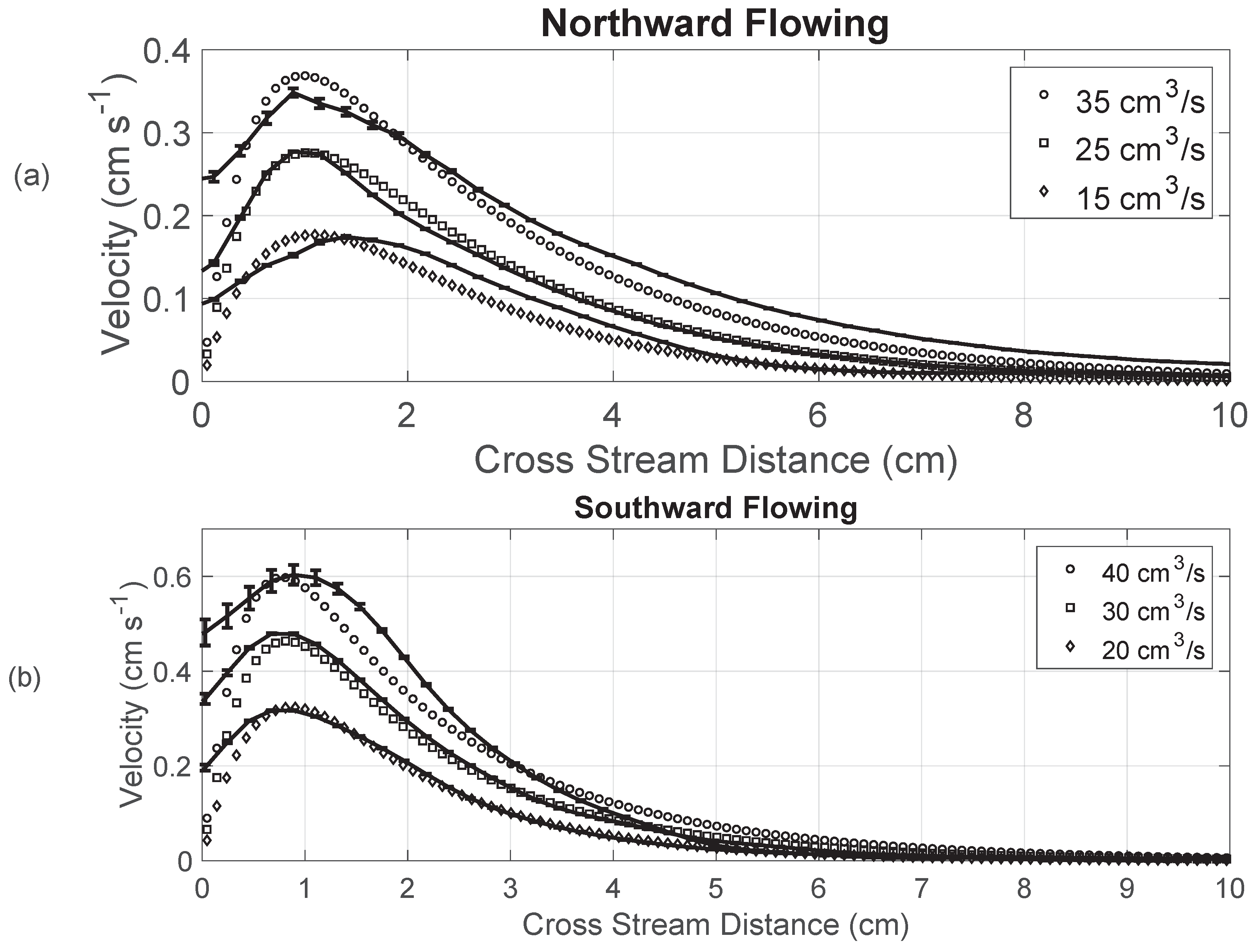
Figure 2 shows the numerical-experimental comparison between northward (top) and southward (bottom) flowing boundary currents. For all cases L D = 5.3 cm, λ S = 0.0197 , and λ M = 0.0241 . Experimental profiles of northward flowing currents with total transports of 35, 25 and 15 cm 3 /s ( R o = 7.7 × 10 4 , 5.5 × 10 4 , 3.3 × 10 4 and λ I = 0.0561 , 0.0474 , 0.0368 ; respectively) are found to be in good agreement with numerical calculations. Experimental profiles of southward flowing currents with total transports of 40, 30 and 20 cm 3 /s ( R o = 8.87 × 10 4 , 6.65 × 10 4 , 4.4 × 10 4 and λ I = 0.0600 , 0.0520 , 0.0424 ; respectively) are also found to be in good agreement with numerical calculations. While the agreement between numerical and experimental profiles is, in general, good, there are noticeable differences. These difference are primarily due to the non-ideal aspects of the experimental setup. For instance, in Figure 1 (panel b), the slight bowing of the isobaths, due to a parabolic layer interface which is indicated in the left panel, is not accounted for. While the numerical solutions account for the parabolic interface, a slight boundary current is formed along the southern tank wall in the experiments, due to the intersection of isobaths with that wall. Thus, the northward flowing boundary current comparison is less accurate than the southward flowing boundary current. Also, velocity profiles very near to the wall suffered from enhanced reflection of the laser light at the wall. This resulted in reduced ability of the experimental profiles to accurately resolve near wall velocity structure. However, in general there is good agreement in both velocity magnitude and structure between the numerical and experimental results. In addition, the numerical results agree with the experimental trend of northward flowing currents broadening with increasing transport compared to southward flowing currents that tend to intensify rather than broaden with increasing transport.

5. Summary

The goal of this study was to investigate 1.5-layer western boundary currents with lateral friction. Here, building upon the previous work of Charney, Huang and Kamenkovich, we have derived, solved and validated a new numerical formulation for accounting for viscous, 1.5 layer western boundary current systems. Specifically, we have included finite layer thickness variations (by accounting for, at minimum, the interface paraboloid) which require analysis beyond standard quasigeostrophic theory. Making the boundary layer approximation and the semi-geostrophic assumption, Equation (3) can be integrated to calculate the finite layer thickness (Equation (4)). Thus, with η and Ψ specified at the inflow boundary, Equation (7) can essentially be solved as a 1D structure function for the viscous 1.5-layer western boundary current problem.

Author Contributions

Conceptualization, C.W.M., J.J.K. and V.A.S.; methodology, C.W.M., J.J.K. and V.A.S.; formal analysis, C.W.M., J.J.K. and V.A.S.; investigation, C.W.M., J.J.K. and V.A.S.; writing–original draft preparation, C.W.M., J.J.K. and V.A.S.; writing–review and editing, C.W.M., J.J.K. and V.A.S.; visualization, C.W.M. and J.J.K.; funding acquisition, J.J.K. All authors have read and agreed to the published version of the manuscript.

Funding

This research was funded by the USA National Science Foundation grant number 1823452.

Conflicts of Interest

The authors declare no conflict of interest. The funders had no role in the design of the study; in the collection, analyses, or interpretation of data; in the writing of the manuscript, or in the decision to publish the results.

References

  1. Prandtl, L. Über Flüssigkeitsbewegung bei sehr kleiner Reibung. Verhandlinger 3. Int. Math. Kongr. Heidelberg 1904, 2, 484–491. [Google Scholar]
  2. Blasius, H. Grenzschichten in Flüssigkeiten mit kleiner Reibung. Z. Angew. Math. Phys. 1908, 56, 1–37. [Google Scholar]
  3. Stommel, H. The westward intensification of wind-driven ocean currents. Trans. AGU 1948, 29, 202. [Google Scholar] [CrossRef]
  4. Munk, W. On the wind-driven ocean circulation. J. Meteorol. 1950, 7, 79–93. [Google Scholar] [CrossRef]
  5. Schlichting, H. Grenzschicht-Theorie; Verlag G. Braun: Karlsruhe, Germany, 1951. [Google Scholar]
  6. Pedlosky, J. Geophyscal Fluid Dynamics, 2nd ed.; Springer: Berlin, Germany, 1987. [Google Scholar]
  7. Il’in, A.M.; Kamenkovich, V.M. The influence of friction on ocean currents. Dokl. Akad. Nauk SSSR 1963, 150, 1274–1277. [Google Scholar]
  8. Il’in, A.M.; Kamenkovich, V.M. The structure of the boundary layer in the two-dimensional theory of ocean currents. Okeanologiya 1964, 4, 756–769. [Google Scholar]
  9. Kamenkovich, V.M. A contribution to the theory of the inertial-viscous boundary layer in a two-dimensional model of ocean currents. Izvestiya, Atmosp. Ocean Phys. 1966, 2, 1274–1295. [Google Scholar]
  10. Ierley, G.R.; Ruehr, O.G. Analytic and Numerical Solutions of a Nonlinear Boundary-Layer Problem. Stud. Appl. Math. 1986, 75, 1–36. [Google Scholar] [CrossRef]
  11. Mallier, R. On The Parametric Model of Western Boundary Outflow. Stud. Appl. Math. 1994, 91, 17–25. [Google Scholar] [CrossRef]
  12. Charney, J.G. The Gulf Stream as an inertial boundary layer. Proc. Natl. Acad. Sci. USA 1955, 41, 731–740. [Google Scholar] [CrossRef] [PubMed] [Green Version]
  13. Huang, R.X. On the structure of inertial western boundary currents with two moving layers. Tellus A 1990, 42, 594–604. [Google Scholar] [CrossRef]
  14. Sheremet, V.A.; Kuehl, J. Gap-Leaping Western Boundary Current in a Circular Tank Model. J. Phys. Oceanogr. 2007, 37, 1488–1495. [Google Scholar] [CrossRef]
  15. Kuehl, J.J.; Sheremet, V.A. Identification of a cusp catastrophe in a gap-leaping western boundary current. J. Mar. Res. 2009, 67, 25–42. [Google Scholar] [CrossRef]
  16. Kuehl, J.J.; Sheremet, V.A. Two-layer gap-leaping oceanic boundary currents: Experimental investigation. J. Fluid Mech. 2014, 740, 97–113. [Google Scholar] [CrossRef]
  17. Hughes, C.W. A theoretical reason to expect inviscid western boundary currents in realistic oceans. Ocean Modell. 2000, 2, 73–83. [Google Scholar] [CrossRef]
  18. Hughes, C.W.; de Cuevas, B.A. Why Western Boundary Currents in Realistic Oceans are Inviscid: A Link between Form Stress and Bottom Pressure Torques. J. Phys. Oceanogr. 2001, 31, 15. [Google Scholar] [CrossRef]
  19. Pierini, S.; Malvestuto, V.; Siena, G.; McClimans, T.A.; Løvås, S.M. A Laboratory Study of the Zonal Structure of Western Boundary Currents. J. Phys. Oceanogr. 2008, 38, 1073–1090. [Google Scholar] [CrossRef]
  20. Pierini, S.; Falco, P.; Zambardino, G.; McClimans, T.A.; Ellingsen, I. A Laboratory Study of Nonlinear Western Boundary Currents, with Application to the Gulf Stream Separation due to Inertial Overshooting*. J. Phys. Oceanogr. 2011, 41, 2063–2079. [Google Scholar] [CrossRef]
  21. Salmon, R. A two-layer Gulf Stream over a continental slope. J. Mar. Res. 1992, 50, 341–365. [Google Scholar] [CrossRef]
  22. Beal, L.M.; Bryden, H.L. The velocity and vorticity structure of the Agulhas Current at 32°S. J. Geophys. Res. 1999, 104, 5151–5176. [Google Scholar] [CrossRef]
  23. Cushman-Roisin, B.; Beckers, J.M. Introduction to Geophysical Fluid Dynamics: Physical and Numerical Aspects, 2nd ed.; Number v. 101 in International Geophysics Series; Academic Press: Waltham, MA, USA, 2011; OCLC: ocn751829434. [Google Scholar]
Figure 1. Two-layer rotating fluid tank setup with axis of rotation through the center of the tank. (a) Side view of two-layer system with sloping lid and bottom shown along with interfacial displacement induced by fluid motion. The solid line represents the layer interface in solid body rotation, while dashed line represents the layer interface with driven flow. (b) Top view for a northward flowing current, which forms at the x = 0 boundary. Dashed lines are isobaths. (c) Numerical flow solution for a northward flowing boundary current.
Fluids 05 00063 g001
Figure 2. Comparison between experimental, solid line with error bars representing standard error, and numerical, open symbols, western boundary current velocity profiles for northward (a) and southward (b) flowing currents.
Fluids 05 00063 g002

