Theoretical Foundation of Rapid Distortion Theory on Transversely Sheared Mean Flows

Abstract

The focus of this paper is on Rapid Distortion Theory on transversely sheared mean flows, which is often used to investigate turbulence-solid surface interactions. The main purpose of the paper is to bring together and present in a consistent fashion a general theory that has been developed in several different papers that have been published in the Journal of Fluid Mechanics. The equations for the unsteady pressure and velocity flections (which decouple from the entropy fluctuations) are rewritten in terms of a gauge function in order to obtain expressions that involve two arbitrarily convected quantities. A pair of very general conservation laws are used to derive upstream boundary conditions that relate these quantities to the actual physical variables. The entropy fluctuations can be determined after the fact once the solutions for the pressure and velocity fluctuations are known. The result involves a third arbitrary convected quantity that is equal to the entropy fluctuations at upstream infinity and can, therefore, be specified as an additional upstream boundary condition. A secondary purpose of the paper is to summarize a number of applications of the theory that have also appeared in the literature and show how they compare with an experiment.

1. Introduction

The interaction of turbulent shear flows with solid surfaces is clearly of great engineering interest [1,2,3] and too many papers have been written on the subject to be listed here. So, we mention only the well-known paper by Tufts, Wang and Wang [2] who used numerical methods to analyze the acoustic radiation produced by the interaction of an aerofoil with a turbulent shear layer. However, these types of interactions can also be studied analytically by using Rapid Distortion Theory (RDT).

RDT was developed to analyze relatively fast changes in turbulent flows such as those that occur in turbulence/solid surface interactions. It applies when the turbulence intensity is small and the interactions take place over length (or time) scales that are short compared to the decay time (or length) of the turbulent eddies [4,5,6,7,8]. These requirements make it possible to identify a distance that is very large (in fact, infinitely large when interpreted asymptotically) on the interaction scale, but still small on the length scale over which the turbulent eddies decay. The resulting flow will then be inviscid and non-heat conducting and will therefore be governed by the Euler equations linearized about an arbitrary nonlinear solution (often referred to as the base flow) to those equations.

1.1. The Kovasznay Result

The basic ideas are best understood by considering a uniform base flow. This case was first analyzed in the seminal paper by Kovasznay [9] which decomposed the unsteady isentropic motion on this flow into a vortical component that carries no pressure fluctuations and a solenoidal component that accounts for the pressure fluctuations. Möhring [10] pointed out that the latter, which is determined by a second-order wave equation in compressible flows, accounts for the acoustic component of the motion of these flows [10]. The former, which is a purely convected quantity in the sense that it moves downstream at the mean flow velocity, can then be interpreted as the hydrodynamic part of the motion. Two of its velocity components can be arbitrarily specified as (usually time-stationary) upstream boundary conditions for the unsteady motion. The Kovasznay decomposition has turned out to be very useful for analyzing turbulence/solid surface interactions on uniform mean flows [11,12,13], or on flows that become uniform far upstream [4,5,6], since the hydrodynamic component of the solution can be used to represent the incident turbulence in these analyses.

1.2. The Orr Result

The analysis becomes much more interesting when the entire base flow is allowed to be non-uniform. The simplest case is arguably a two-dimensional and incompressible flow with uniform mean shear so that the mean velocity, say $U$, is of the form

$$U=\mathrm{\Lambda }{y}_2,$$

(1)

with constant $\mathrm{\Lambda }\equiv dU/d{y}_2$ and $\left\{y_1,y_2,y_3\right\}$ denoting Cartesian coordinates, with $y_1$ in the mean flow direction. The unsteady motion is then determined by the linearized incompressible vorticity equation (the compressible case was analyzed by Möhring [10])

$$\left(\partial /\partial \tau +U\partial /\partial y_1\right){{\omega }^{\prime }}_3=0$$

(2)

with $\tau$ denoting the time and ${{\omega }^{\prime }}_3$ denoting the spanwise vorticity perturbation. It was first pointed out by Orr [14,15] that Equation (2) or, equivalently, the two-dimensional Rayleigh equation

$$\frac{\partial }{\partial y_1}\left(\frac{\partial }{\partial \tau }+U\frac{\partial }{\partial y_1}\right){{\omega }^{\prime }}_3=\left(\frac{\partial }{\partial \tau }+U\frac{\partial }{\partial y_1}\right)\left(\frac{{\partial }^2}{\partial y_1^2}+\frac{{\partial }^2}{\partial y_2^2}\right){v^{\prime }}_2=0,$$

(3)

which determines the unsteady cross-gradient velocity perturbation, ${v^{\prime }}_2\left(y_2,\tau \right)$, can be integrated to show that the spanwise vorticity perturbation ${{\omega }^{\prime }}_3$ can be an arbitrary function, say ${\omega }_c\left(\tau -y_1/\mathrm{\Lambda }{y}_2,y_2\right)$, of the indicated arguments and that ${v^{\prime }}_2$ is determined by

$$\left(\frac{{\partial }^2}{\partial y_1^2}+\frac{{\partial }^2}{\partial y_2^2}\right){v^{\prime }}_2=\frac{\partial }{\partial y_1}{\omega }_c\left(\tau -\frac{y_1}{\mathrm{\Lambda }{y}_2},y_2\right),$$

(4)

Orr [14] calculated the velocity and pressure fluctuations evolving from an initial state by solving an initial value problem associated with this equation. However, these solutions (or their long time limits) are not all that relevant to the time-stationary turbulent flows being considered here since the corresponding solutions to the full nonlinear equations can develop internal shear layers that can no longer be treated inviscidly and can support Kelvin–Helmholtz instabilities [16,17,18]. It is, however, not unreasonable to use the time-stationary or steady-state solutions given by Equation (4) to represent the turbulence in these flows. The relevant solution can then be written as

$${v^{\prime }}_2\left(\mathit{x},t\right)=\frac{\partial }{\partial x_1}{\displaystyle \underset{-T}{\overset{T}{\int }}{\displaystyle \underset{}{\int }{G}_{\perp }\left(\mathit{x},t|\mathit{y},\tau \right){\omega }_c\left(\tau -\frac{y_1}{\mathrm{\Lambda }{y}_2},y_2\right)}}d\mathit{y}d\tau ,$$

(5)

where $\mathit{x}=\left\{x_1,x_2\right\}$ and $\mathit{y}=\left\{y_1,y_2\right\}$ are two-dimensional Cartesian coordinates, $T$ represents a large time interval and $G_{\perp }$ denotes the two-dimensional Green’s function that is determined by the equation

$$\left(\frac{{\partial }^2}{\partial x_1^2}+\frac{{\partial }^2}{\partial x_2^2}\right)G_{\perp }\left(\mathit{x},t|\mathit{y},\tau \right)=\delta \left(t-\tau \right)\delta \left(\mathit{y}-\mathit{x}\right)$$

(6)

together with appropriate boundary conditions. The vorticity ${{\omega }^{\prime }}_3$, which is equal to the convected quantity ${\omega }_c\left(\tau -y_1/U\left(y_2\right),y_2\right)$, can now be specified as a boundary condition since Equation (5) will satisfy Equation (4) for any choice of this quantity.

The inner integral in Equation (5) is assumed to be carried out over an unbounded or semi-bounded region of space, with the Green’s function $G_{\perp }$ required to satisfy appropriate transverse boundary conditions in the latter case and taken to be the free space Green’s function ${\left(4\pi \right)}^{-1}\ln {\left|\mathit{x}-\mathit{y}\right|}^2\delta \left(t-\tau \right)$ in the former case. The transverse velocity perturbation ${v^{\prime }}_2\left(\mathit{x},t\right)$ will then be given by [19]

$${v^{\prime }}_2\left(\mathit{x},t\right)={\displaystyle \underset{-\infty }{\overset{\infty }{\int }}}{\overline{G}}_{\perp }\left(x_2|y_2\right){\omega }_c\left(t-x_1/\mathrm{\Lambda }{y}_2\right)d{y}_2$$

(7)

with

$${\overline{G}}_{\perp }\left(x_2|y_2\right)\equiv \frac{i}{2}\left(\mathrm{sgn}\omega \right)\left(\mathrm{sgn}{y}_2\right)e^{-\left|\omega \right|\left|x_2-y_2\right|/\mathrm{\Lambda }\left|y_2\right|}$$

(8)

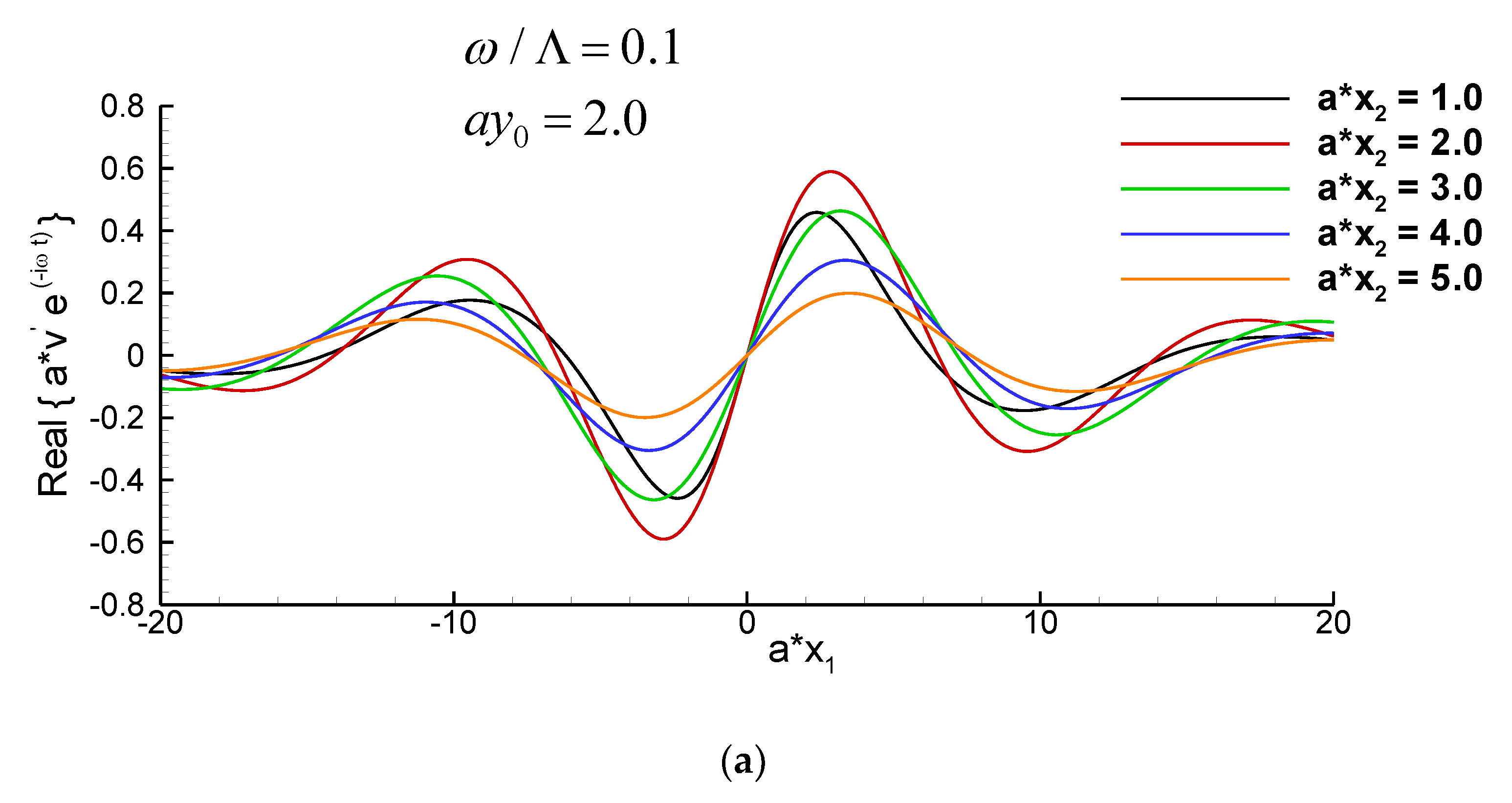
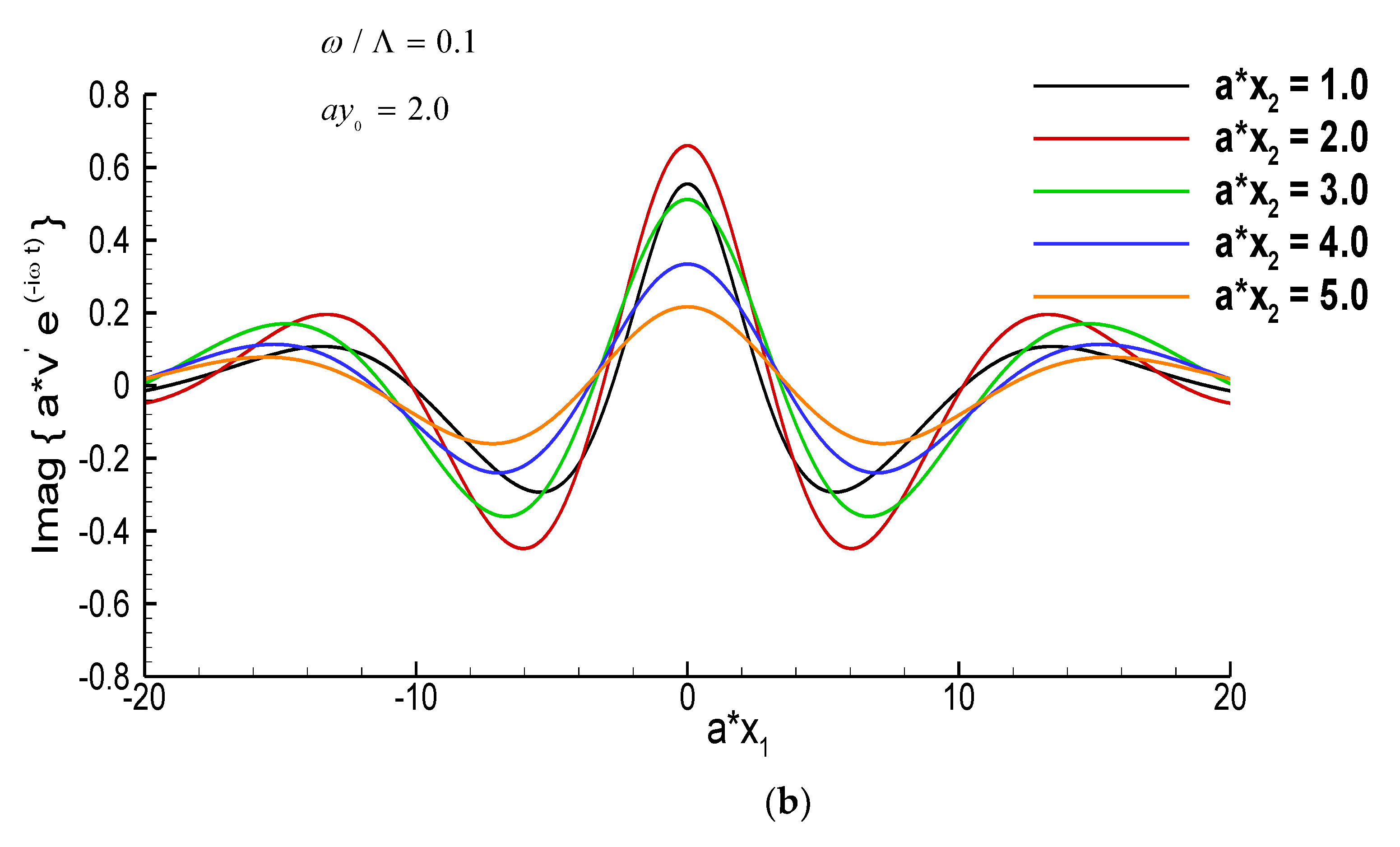
when the convected vorticity ${\omega }_c\left(\tau -y_1/U\left(y_2\right),y_2\right)$ is taken to be the generic time-harmonic function

$${\omega }_c\left(t-\frac{y_1}{U\left(y_2\right)},y_2\right)=e^{i\omega \left[t-y_1/U\left(y_2\right)\right]}{\tilde{\mathsf{\Omega }}}_c\left(y_2:\omega \right)$$

(9)

Figure 1, which is a plot of some typical values of ${v^{\prime }}_2$ calculated from Equations (7)–(9) with ${\tilde{\mathsf{\Omega }}}_c\left(y_2:\omega \right)$ taken to be

$${\tilde{\mathsf{\Omega }}}_c\left(y_2:\omega \right)=e^{-{\left[a\left(y_2-y_0\right)\right]}^2},$$

(10)

shows that this quantity differs from the corresponding Kovasznay result on a uniform mean flow in that it now decays as $x_1\to \pm \infty$.

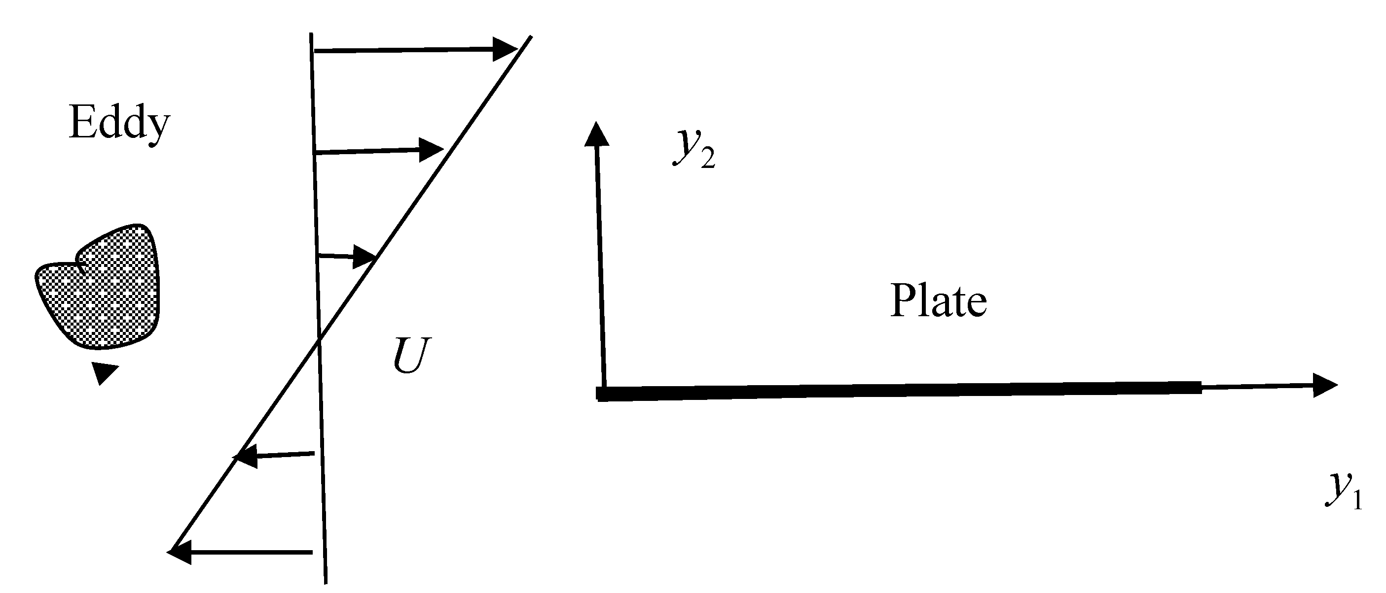
This behavior will also occur in surface interaction problems, which might arise when a flat plate with a leading edge at $y_1=0$ is placed in the flow (see Figure 2). These considerations show that it is not possible to impose upstream boundary conditions by specifying ${v^{\prime }}_2$ at the upstream infinity for this type of problem. However, it follows from Equation (4) that the Laplacian $\left({\partial }^2/\partial y_1^2+{\partial }^2/\partial y_2^2\right){v^{\prime }}_2$ is equal to the streamwise derivative of the convected quantity ${\omega }_c\left(\tau -y_1/U\left(y_2\right),y_2\right)$ and, therefore, does not decay. This means that the former quantity can be specified far upstream (infinitely far in an asymptotic sense) on the interaction length scale, which can still be small (infinitely small in an asymptotic sense) compared to the scale on which the turbulence evolves.

The key result is that the arbitrary function ${\omega }_c\left(\tau -y_1/U\left(y_2\right),y_2\right)$ can be determined by specifying an actual physical variable in a region where the flow is unaffected by the solid surface. The present paper shows that the situation is analogous but much more interesting for more complicated transversely sheared flows.

1.3. Scope of the Paper

A large number of papers [7,8,21,22] have used locally homogeneous RDT, which is a kind of local high-frequency approximation first introduced by Moffatt [23], to study the turbulent motion on planar shear flows. The assumption of local homogeneity eliminates the requirement for upstream boundary conditions, but the present paper is only concerned with non-homogenous RDT, which usually provides a much more realistic description of the flow. There are also a large number of papers on this subject that have appeared in the literature, but the focus of the present paper is on the much narrower topic of non-homogenous RDT on transversely sheared mean flows. Its primary purpose is to bring together and describe in an integrated fashion a general methodology that has been developed in a number of different papers [5,6,20,21] to deal with this phenomenon. Some significant new results are also presented.

The basic equations are rewritten in terms of a gauge function in Section 3 and a formal solution to the complete inhomogeneous RDT problem is given in Section 4. Section 5 discusses the role of causality and instability waves and shows that (as in the Kovasznay decomposition) the resulting formulas for the unsteady pressure and velocity fluctuations (which decouple from the entropy fluctuations) involve two convected quantities. However, unlike the Kovasznay result, they are not directly related to the physical flow variables. However, it is shown that they can be linked to these variables by using two very general conservation laws (derived in Appendix A and discussed in Section 7) that relate the convected quantities to the physical variables and a gradient-wise particle displacement (defined in Section 5). Appendix B shows that the latter quantity vanishes at upstream infinity and, therefore (as shown in Section 8), that conservation laws can be used to obtain a set of upstream boundary conditions that relate the convected quantities to the physical variables.

Spatially growing instability waves- which are usually associated with coherent structures in turbulent flows-may also appear in the solutions. However, their amplitudes cannot be determined by imposing upstream boundary conditions since they decay exponentially fast at upstream infinity. They can, however, be determined as part of the solution when causality is imposed on the flow, which appears to be particularly appropriate in the present context since Creighton [24,25] has shown that the imposition of causality is equivalent to imposing a Kutta condition at a trailing edge.

Section 6 shows that the entropy fluctuations can be determined from the particle displacement once the solution for the pressure and velocity fluctuations is known. The result brings in a third arbitrary convected function, which is equal to the entropy fluctuations at upstream infinity and can, therefore, be specified as a third upstream boundary condition.

Section 9 shows how these results can be used to relate turbulent pressure spectrum (which is of principal interest in acoustic and structural vibration problems) to the upstream turbulent velocity spectrum (usually specified as an upstream boundary condition in turbulent surface interaction problems) and an appropriate model for this spectrum is introduced. Some applications of the theory that have appeared in the literature are described in Section 11 and some brief conclusions are given in Section 12.

2. The Basic Equations

We consider the flow of an inviscid and non-heat conducting fluid which is assumed to be an ideal gas with squared sound speed $\gamma p/\rho$, and entropy $c_v\ln \left(p/{\rho }^{\gamma }\right)$ where $p$ and $\rho$ denote the pressure and density, respectively, and $\gamma$ denotes the specific heat ratio $c_p/c_v$ where $c_p,c_v$ are the specific heats at constant pressure and volume, respectively.

The pressure $p^{\prime }=p-p_0$ and mass flux

$$\mathit{u}=\left\{u_1,u_2,u_3\right\}\equiv \rho \left\{{v^{\prime }}_1,{v^{\prime }}_2,{v^{\prime }}_3\right\}$$

(11)

perturbations (where $\mathit{v}\text{′}=\left\{{v^{\prime }}_1,{v^{\prime }}_2,{v^{\prime }}_3\right\}$ is the actual velocity perturbation) on a transversely sheared mean flow whose velocity $U\left({\mathit{y}}_T\right)$ is in a single direction, whose pressure $p_0$ is equal to a constant, and whose mean sound speed squared $c^2\left({\mathit{y}}_T\right)$ depends only on the transverse coordinate ${\mathit{y}}_T$, decouple from the entropy fluctuations and are governed by the linearized momentum and continuity equations

$$\frac{D_0{u}_i}{D\tau }+{\delta }_{1i}{u}_j\frac{\partial U}{\partial y_j}+\frac{\partial }{\partial y_i}{p}^{\prime }=0, i=1,2,3$$

(12)

and

$$u_i\frac{D_0{p}^{\prime }}{D\tau }+\frac{\partial }{\partial y_j}{c}^2{u}_j=0$$

(13)

where ${\mathit{y}}_T\equiv \left\{y_2,y_3\right\}$, $\mathit{y}\equiv \left\{y_1,y_2,y_3\right\}=\left\{y_1,{\mathit{y}}_T\right\}$ and

$$\frac{D_0}{D\tau }\equiv \frac{\partial }{\partial \tau }+U\left({\mathit{y}}_T\right)\frac{\partial }{\partial y_1}$$

(14)

denote the convective derivative based on the source point (while $D_0/Dt\equiv \partial /\partial t+U\left({\mathit{x}}_T\right)\partial /\partial x_1$ denotes the convective derivative based on the observation point).

The entropy fluctuation $s^{\prime }$ depends on the momentum fluctuations and can be determined from the energy equation (Equation (11) of [26])

$$\frac{D_0{s}^{\prime }}{D\tau }=\frac{c_p}{{\rho }_0^2}{u}_i\frac{\partial {\rho }_0}{\partial y_i}$$

(15)

once $u_i$ is known.

3. The Gauge Function Representation

The momentum Equation (12) will be identically satisfied for any arbitrary function $\varphi$ and any purely convected function $\vartheta \left(\tau -\left(y_1/U\right),{\mathit{y}}_T\right)$ when the pressure fluctuation $p^{\prime }$ and the momentum fluctuation.$u_i$ are related to $\vartheta$ and $\varphi$ by [27]

$$p^{\prime }=-\frac{D_0^3\varphi }{D{\tau }^3},$$

(16)

and

$$u_i=\frac{D_0}{D\tau }{\lambda }_i-{\delta }_{1i}\frac{\partial U}{\partial y_j}{\lambda }_j+{\epsilon }_{ijk}\frac{1}{c^2}\frac{\partial U}{\partial y_j}\frac{\partial }{\partial y_k}\vartheta \left(\tau -\frac{y_1}{U},{\mathit{y}}_T\right),\mathrm{for}i=1,2,3,$$

(17)

where $\varphi$ plays the role of a gauge function,

$${\lambda }_j\equiv \frac{\partial }{\partial y_j}\frac{D_0\varphi }{D\tau }+2\frac{\partial U}{\partial y_j}\frac{\partial \varphi }{\partial y_1}$$

(18)

is a kind “pseudo-particle displacement”, ${\delta }_{ij}$ denotes the Kronecker delta and ${\epsilon }_{ijk}$ denotes the Levi–Cevita permutation tensor.

Since the Gauge function $\varphi$ is undetermined at this stage of the analysis it can be adjusted to ensure that the continuity Equation (13) is also satisfied by substituting Equations (16)–(18) into Equation (13) to obtain

$$\frac{D_0}{D\tau }{L}_a\varphi =0,$$

(19)

where $L_a$ denotes the linear operator

$$L_a\equiv \frac{D_0^3}{D{\tau }^3}-\frac{\partial }{\partial y_i}{c}^2\left(\frac{\partial }{\partial y_i}\frac{D_0}{D\tau }+2\frac{\partial U}{\partial y_i}\frac{\partial }{\partial y_1}\right)$$

(20)

As in the Orr analysis discussed in Section 1.2, this result can be integrated to show that the gauge function $\varphi$ is determined by

$$L_a\varphi =-{\tilde{\omega }}_c\left(\tau -\frac{y_1}{U},{\mathit{y}}_T\right)$$

(21)

where ${\tilde{\omega }}_c\left(\tau -y_1/U,{\mathit{y}}_T\right)$ denotes a second arbitrary convected quantity.

4. Green’s Function Solution of Gauge Function Equation

Eliminating the mass flux perturbation $\mathit{u}$ between Equations (12) and (13) shows that the pressure fluctuation $p^{\prime }$ satisfies the well-known Rayleigh’s equation [28]

$$L{p}^{\prime }=0,$$

(22)

where

$$L\equiv \frac{D_o}{D\tau }\left(\frac{\partial }{\partial y_i}{c}^2\frac{\partial }{\partial y_i}-\frac{D_o^2}{D{\tau }^2}\right)-2\frac{\partial U}{\partial y_j}\frac{\partial }{\partial y_1}{c}^2\frac{\partial }{\partial y_j}$$

(23)

denotes the usual Rayleigh operator, which turns out to be adjoint to the operator $L_a$ defined by Equation (20) since

$$\overline{v}L\overline{u}-\overline{u}{L}_a\overline{v}=\frac{\partial }{\partial y_i}{c}^2\left(\overline{u}\frac{\partial }{\partial y_i}\frac{D_0\overline{v}}{D\tau }+2\overline{u}\frac{\partial U}{\partial y_i}\frac{\partial \overline{v}}{\partial y_1}-\frac{\partial \overline{u}}{\partial y_i}\frac{D_0\overline{v}}{D\tau }\right)$$

$$+\frac{D_0}{D\tau }\left(\overline{v}\frac{\partial }{\partial y_i}{c}^2\frac{\partial \overline{u}}{\partial y_i}+\frac{D_0\overline{u}}{D\tau }\frac{D_0\overline{v}}{D\tau }-\overline{u}\frac{D_0^2\overline{v}}{D{\tau }^2}-\overline{v}\frac{D_0^2\overline{u}}{D{\tau }^2}\right)-2\frac{\partial }{\partial y_1}\left(c^2\frac{\partial U}{\partial y_j}\overline{v}\frac{\partial \overline{u}}{\partial y_j}\right)$$

(24)

for any functions $\overline{u},\overline{v}$ [29].

Since, to our knowledge, all applications of non-homogeneous RDT have been to steady-state turbulent flows the focus here will be on the time-stationary solutions of Equation (21), we, therefore, suppose that $\varphi$ is time stationary [30] and that initial conditions imposed in the distant past do not affect the solution at the finite time $t$.

Let $g\left(\mathit{y},\tau |\mathit{x},t\right)$ denote the Green’s function for the Rayleigh operator $L$ that satisfies

$$Lg\left(\mathit{y},\tau |\mathit{x},t\right)=\delta \left(\mathit{y}-\mathit{x}\right)\delta \left(\tau -t\right),$$

(25)

and behaves like an incoming wave as $\left|\mathit{y}\right|\to \infty$. As usual we let the first two arguments of $g\left(\mathit{y},\tau |\mathit{x},t\right)$ represent the dependent variables and let the second two represent the source variables. Since $g\left(\mathit{y},\tau |\mathit{x},t\right)$ denotes value of the solution to Equation (25) at $\left(\mathit{y},\tau \right)$ due to a point sink at $\left(\mathit{x},t\right)$, it should be related to its adjoint $g_a\left(\mathit{x},t|\mathit{y},\tau \right)$ by the reciprocity relation [29,31]

$$g\left(\mathit{y},\tau |\mathit{x},t\right)=g_a\left(\mathit{x},t|\mathit{y},\tau \right)$$

(26)

Then since $g_a\left(\mathit{x},t|\mathit{y},\tau \right)$ satisfies Equation (21) with the source function $-{\tilde{\omega }}_c\left(\tau -y_1/U,{\mathit{y}}_T\right)$ replaced by $\delta \left(\mathit{y}-\mathit{x}\right)\delta \left(\tau -t\right),$ and, therefore, corresponds to a direct Green’s function in the present context, it reasonable to require that it satisfy the causality condition $g_a\left(\mathit{x},t|\mathit{y},\tau \right)=0,\mathrm{for}\mathrm{all}\mathit{t}\text{<}\tau$, which implies that the Green’s function, $g\left(\mathit{y},\tau |\mathit{x},t\right)$, will vanish for all finite $\mathit{y}$ as $\tau \to \infty$, since it vanishes for all $\tau >t$ by definition.

We can require that the solution $\varphi \left(\mathit{x},t\right)$ of the gauge function defined by Equation (21) along with its derivatives (and, therefore, the pressure fluctuations) vanish (for all finite times) as $x_1$ goes to plus or minus infinity when the source function ${\tilde{\omega }}_c$ is reasonably compact—even for globally unstable base flows since the signal generated at $\left(\mathit{y},\tau \right)$ cannot reach these locations when $t=T$ is finite. This means that gauge function $\varphi \left(\mathit{y},\tau \right)$ goes to zero as $y_1\to \pm \infty$ for all finite $\tau$. We also assume that the initial conditions are such that $\varphi \left(\mathit{y},\tau \right)$ and its derivatives vanish for all finite $\mathit{y}$ as $\tau \to -\infty$.

Setting $\overline{u}$ equal to $g\left(\mathit{y},\tau |\mathit{x},t\right)$ in Equation (24), letting $\overline{v}$ denote a solution to Equation (21) and using the divergence theorem shows that Equation (21) possess the formal steady-state solution [27]

$$\varphi \left(\mathit{x},t\right)=-{\displaystyle \underset{-T}{\overset{T}{\int }}{\displaystyle \underset{V}{\int }g\left(\mathit{y},\tau |x,t\right){\tilde{\omega }}_c\left(\tau -\frac{y_1}{U\left({\mathit{y}}_T\right)},{\mathit{y}}_T\right)}}d\mathit{y}d\tau$$

$$+{\displaystyle \underset{-T}{\overset{T}{\int }}{\displaystyle \underset{S}{\int }{\widehat{n}}_j{c}^2\left[g\left(\mathit{y},\tau |x,t\right){\lambda }_j-\frac{\partial g\left(\mathit{y},\tau |x,t\right)}{\partial y_j}\frac{D_0\varphi }{D\tau }\right]}}dS\left(\mathit{y}\right)d\tau$$

(27)

where $T$ is a large but finite time, the volume $V$ is assumed to be bounded by cylindrical surface(s) $S$ that can be of finite, semi-infinite or infinite length in the streamwise direction, $\widehat{n}=\left\{{\widehat{n}}_i\right\}$ denotes the unit outward-drawn normal to $S$ and ${\lambda }_j$ is defined by Equation (18). Since $g\left(\mathit{y},\tau |\mathit{x},t\right)=0$ for $\tau >t$ we can replace the upper limit $T$ by the time $t$.

Equation (27) expresses the solution to Equation (21) in terms of the volume source distribution ${\tilde{\omega }}_c\left(\tau -y_1/U\left({\mathit{y}}_T\right),{\mathit{y}}_T\right)$ and the gauge function $\varphi$ distribution over one or more cylindrical surfaces $S$. The formulation is unconventional since the direct Green’s function $g$ now plays the role of an adjoint Green’s function in the solution of Equation (27) for the Gauge function $\varphi$. The surface integral will not appear in Equation (27) and the Green’s function $g$ will be completely determined by Equation (25) together with the causality requirements given above when the integration volume $V$ is all of space and will be incompletely determined by these requirements when it is not.

5. Integral Solution for the Physical Variables

5.1. The Pressure Fluctuation

Substituting Equation (27) into Equation (16) shows that the pressure fluctuation $p^{\prime }$ is given by

$$p^{\prime }\left(\mathit{x},t\right)={\displaystyle \underset{-T}{\overset{T}{\int }}{\displaystyle \underset{V}{\int }G\left(\mathit{y},\tau |x,t\right){\tilde{\omega }}_c\left(\tau -\frac{y_1}{U\left({\mathit{y}}_T\right)},{\mathit{y}}_T\right)}}d\mathit{y}d\tau$$

$$-{\displaystyle \underset{-T}{\overset{T}{\int }}{\displaystyle \underset{S}{\int }{\widehat{n}}_j{c}^2\left[G\left(\mathit{y},\tau |x,t\right){\lambda }_j-\frac{\partial G\left(\mathit{y},\tau |x,t\right)}{\partial y_j}\frac{D_0\varphi }{D\tau }\right]}}dS\left(\mathit{y}\right)d\tau$$

(28)

where

$$G\left(\mathit{y},\tau |\mathit{x},t\right)\equiv \frac{D_0^{3}g\left(\mathit{y},\tau |x,t\right)}{D{t}^3}$$

(29)

satisfies the reduced Rayleigh Green’s function equation [27]

$$L\mathit{G}\left(\mathit{y},\tau |\mathit{x},t\right)=\frac{D_0^3}{D{t}^3}\delta \left(\mathit{y}-\mathit{x}\right)\delta \left(\tau -t\right)$$

(30)

Equation (28) can be rewritten as

$$p^{\prime }\left(\mathit{x},t\right)={\displaystyle \underset{-T}{\overset{T}{\int }}{\displaystyle \underset{V}{\int }G\left(\mathit{y},\tau |x,t\right){\tilde{\omega }}_c\left(\tau -\frac{y_1}{U\left({\mathit{y}}_T\right)},{\mathit{y}}_T\right)}}d\mathit{y}d\tau$$

$$-{\displaystyle \underset{-T}{\overset{T}{\int }}{\displaystyle \underset{S}{\int }\left[G\left(\mathit{y},\tau |x,t\right)\left({\widehat{n}}_j{c}^2{\lambda }_j\right)+\mathsf{\Gamma }\left(\mathit{y},\tau |x,t\right)p^{\prime }\left(\mathit{y},\tau \right)\right]}}dS\left(\mathit{y}\right)d\tau$$

(31)

by introducing the variable $\mathsf{\Gamma }\left(\mathit{y},\tau |\mathit{x},t\right)$ defined to within some arbitrary convected quantities by

$$\frac{D_0^2\mathsf{\Gamma }\left(\mathit{y},\tau |x,t\right)}{D{\tau }^2}\equiv {\widehat{n}}_j{c}^2\frac{\partial G\left(\mathit{y},\tau |x,t\right)}{\partial y_j},\mathit{y}\in S$$

(32)

and integrating by parts. Goldstein et al. [27] used this result to extend Equation (28) to flows with discontinuous velocity profiles downstream of the solid surfaces. They showed that the transverse component of the effective particle displacement $c^2{\widehat{n}}_i{\lambda }_i$ and the pressure perturbation $p^{\prime }$ will be continuous across the discontinuities when $G\left(\mathit{y},\tau |\mathit{x},t\right)$ and $\mathsf{\Gamma }\left(\mathit{y},\tau |\mathit{x},t\right)$ are required to satisfy the jump condition

$$\Delta \left[G\right]=\Delta \left[\mathsf{\Gamma }\right]=0,\mathrm{for}{\mathit{y}}_T\in S_0$$

(33)

where $\Delta [·]$ denotes the jump in the indicated quantity across the surface/surfaces of discontinuity $S_0$ which will correspond to infinitely thin wakes or vortex sheets downstream of the solid surfaces when, as will usually be the case, they coincide with level surfaces of the mean flow.

5.2. Role of Instability Waves

It is well-known that inflectional base flows can support spatially growing instability waves, which are often used to represent the large-scale coherent structures in turbulent flows. Since all these instabilities (other than the singular neutral instability) decay exponentially fast at upstream infinity their amplitudes cannot be determined from by specifying upstream boundary conditions. However, as shown by Briggs [32] and Bers [33], they are uniquely determined as part of the solution when causality is imposed on the flow-which appears to be particularly appropriate in the present context since Creighton [24,25] has shown that the imposition of causality is equivalent to imposing a Kutta condition at the trailing edges.

5.3. The Pseudo-Particle Displacement

As is in the previous case the surface integrals drop out of Equation (31) and the Green’s function $G$ is then completely determined by Equation (30) together with the causality requirements given above when the doubly infinite surfaces $S$ are all at infinity (i.e., when $V$ represents all of space) but they can still be eliminated when they are not at infinity by requiring that $G$ satisfy appropriate boundary conditions on these surfaces. The second term in square brackets drops out of the surface integral when

$$\mathsf{\Gamma }\left(\mathit{y},\tau |\mathit{x},t\right)=0\mathrm{for}\mathit{y}\in S$$

(34)

The remaining term will vanish when

$${\widehat{n}}_i{\lambda }_i{c}^2=0,\mathrm{for}\mathit{y}\in S$$

(35)

and the pressure perturbation $p^{\prime }$ will then be given by

$$p^{\prime }\left(\mathit{x},t\right)={\displaystyle \underset{-T}{\overset{T}{\int }}{\displaystyle \underset{V}{\int }G\left(\mathit{y},\tau |x,t\right){\tilde{\omega }}_c\left(\tau -\frac{y_1}{U\left({\mathit{y}}_T\right)},{\mathit{y}}_T\right)}}d\mathit{y}d\tau$$

(36)

This means that the pressure fluctuation $p^{\prime }$ corresponding to a solution whose surface behavior is consistent with Equation (35) will be determined by Equation (36) when $G$ satisfies Equations (33) and (34). It follows from Equation (17) that consistency with Equation (35) requires that the $\vartheta$-independent component of the density-weighted velocity perturbation

$${\tilde{u}}_i^{}\left(\mathit{x},t\right)\equiv \frac{D_0}{D\tau }{\lambda }_i-{\delta }_{1i}\frac{\partial U}{\partial y_j}{\lambda }_j$$

(37)

vanish on $S$ and, therefore, that the corresponding density-weighted normal surface velocity ${\widehat{n}}_i{u}_i$ is given by

$$c^2{\widehat{n}}_i{u}_i^{}={\epsilon }_{ijk}{\widehat{n}}_i\frac{\partial U}{\partial y_j}\frac{\partial }{\partial y_k}\vartheta \left(\tau -\frac{y_1}{U},{\mathit{y}}_T\right)={\epsilon }_{ij1}{\widehat{n}}_i\frac{\partial U}{\partial y_j}\frac{\partial }{\partial y_1}\vartheta \left(\tau -\frac{y_1}{U},{\mathit{y}}_T\right)\mathrm{for}\mathit{y}\in S$$

(38)

Since the surfaces $S$ must be aligned with the mean flow. In fact they will usually coincide with the level $U=$ constant surfaces: in which case Equation (35) will be equivalent to requiring that the gradient-wise component

$${\lambda }_{\perp }\left(\mathit{y},\tau \right)\equiv \left(\partial U/\partial y_i\right){\lambda }_i=\frac{\partial U}{\partial y_j}\left(\frac{\partial }{\partial y_j}\frac{D_0\varphi }{D\tau }+2\frac{\partial U}{\partial y_j}\frac{\partial \varphi }{\partial y_1}\right)$$

(39)

of the pseudo-particle displacement ${\lambda }_i$ vanish on $S$ and Equation (38) will then imply that the (density-weighted) normal surface velocity ${\widehat{n}}_i{u}_i$ vanishes on $S$, since the normal vector $\hat{\mathit{n}}$ is then equal to $\nabla U/\left|\nabla U\right|$. Equation (38) shows that this will occur even when $S$ does not coincide with a level $U=$ constant surface if

$$\vartheta \left(\tau -\frac{y_1}{U},{\mathit{y}}_T\right)=0\mathrm{for}\mathit{y}\in S$$

(40)

Equations (18) and (27) show that the complete pseudo-particle displacement is given by

$${\lambda }_i=-{\displaystyle \underset{-T}{\overset{T}{\int }}{\displaystyle \underset{V}{\int }{\tilde{G}}_i\left(\mathit{y},\tau |x,t\right){\tilde{\omega }}_c\left(\tau -\frac{y_1}{U\left({\mathit{y}}_T\right)},{\mathit{y}}_T\right)}}d\mathit{y}d\tau$$

$$-{\displaystyle \underset{-T}{\overset{T}{\int }}{\displaystyle \underset{S}{\int }\left[{\tilde{G}}_i\left(\mathit{y},\tau |x,t\right)\left({\widehat{n}}_j{c}^2{\lambda }_j\right)+{\tilde{\mathsf{\Gamma }}}_i\left(\mathit{y},\tau |x,t\right)p^{\prime }\left(\mathit{y},\tau \right)\right]}}dS\left(\mathit{y}\right)d\tau ,\mathrm{for}i=1,2,3$$

(41)

with ${\tilde{G}}_i\left(\mathit{y},\tau |\mathit{x},t\right)$ determined by

$${\tilde{G}}_i\left(\mathit{y},\tau |\mathit{x},t\right)\equiv \frac{\partial }{\partial x_j}\frac{D_{0}g}{Dt}+2\frac{\partial U}{\partial x_j}\frac{\partial g}{\partial x_1},\mathrm{for}i=1,2,3$$

(42)

and is, therefore, related to the Green’s function derivative $\partial G\left(\mathit{y},\tau |\mathit{x},t\right)/\partial x_i$ of $G\left(\mathit{y},\tau |\mathit{x},t\right)$ by

$$\frac{D_0^2}{D{t}^2}{\tilde{G}}_i\left(\mathit{y},\tau |\mathit{x},t\right)=\frac{\partial }{\partial x_i}G\left(\mathit{y},\tau |\mathit{x},t\right),\mathrm{for}i=1,2,3$$

(43)

which means that ${\tilde{\mathsf{\Gamma }}}_i\left(\mathit{y},\tau |\mathit{x},t\right)$ is related to the transverse gradient of ${\tilde{G}}_i\left(\mathit{y},\tau |\mathit{x},t\right)$ by

$$\frac{D_0^2{\tilde{\mathsf{\Gamma }}}_i\left(\mathit{y},\tau |x,t\right)}{D{\tau }^2}\equiv {\widehat{n}}_j{c}^2\frac{\partial {\tilde{G}}_i\left(\mathit{y},\tau |x,t\right)}{\partial y_j}$$

(44)

5.4. The Density-Weighted Gradient-Wise Velocity Perturbation

It now follows from Equation (17) that the density-weighted gradient-wise velocity perturbation

$$u_{\perp }\equiv \frac{1}{\left|\nabla U\right|}\frac{\partial U}{\partial y_i}{u}_i$$

(45)

is related to the transverse particle displacement defined in Equation (39) by

$$u_{\perp }{}_{}=\frac{1}{\left|\nabla U\right|}\frac{D_0{\lambda }_{\perp }}{D\tau },$$

(46)

which is (like $p^{\prime }$) also independent of the second independent convected quantity $\vartheta \left(\tau -y_1/U,{\mathit{y}}_T\right)$ and is explicitly given by

$$u_{\perp }={\displaystyle \underset{-T}{\overset{T}{\int }}{\displaystyle \underset{V}{\int }{G}_{\perp }\left(\mathit{y},\tau |x,t\right){\tilde{\omega }}_c\left(\tau -\frac{y_1}{U\left({\mathit{y}}_T\right)},{\mathit{y}}_T\right)}}d\mathit{y}d\tau$$

$$-{\displaystyle \underset{-T}{\overset{T}{\int }}{\displaystyle \underset{S}{\int }\left[G_{\perp }\left(\mathit{y},\tau |x,t\right)\left({\widehat{n}}_j{c}^2{\lambda }_j\right)+{\mathsf{\Gamma }}_{\perp }\left(\mathit{y},\tau |x,t\right)p^{\prime }\left(\mathit{y},\tau \right)\right]}}dS\left(\mathit{y}\right)d\tau$$

(47)

where $G_{\perp }\left(\mathit{y},\tau |\mathit{x},t\right)$ is defined by

$$G_{\perp }\left(\mathit{y},\tau |\mathit{x},t\right)\equiv -\frac{\nabla U}{\left|\nabla U\right|}·\frac{D_0}{Dt}\left[\nabla \frac{D_0}{Dt}+2\left(\nabla U\right)\frac{\partial }{\partial x_1}\right]g\left(\mathit{y},\tau |\mathit{x},t\right).$$

(48)

with

$$\nabla \equiv \left\{\partial /\partial x_i\right\}.$$

(49)

and is, therefore, related to the gradient of $G\left(\mathit{y},\tau |\mathit{x},t\right)$ by

$$\frac{D_0}{Dt}{G}_{\perp }\left(\mathit{y},\tau |\mathit{x},t\right)=-\frac{\nabla U}{\left|\nabla U\right|}·\nabla G\left(\mathit{y},\tau |\mathit{x},t\right)$$

(50)

The pseudo-particle displacement and gradient-wise velocity perturbation will be given by

$${\lambda }_i=-{\displaystyle \underset{-T}{\overset{T}{\int }}{\displaystyle \underset{V}{\int }{\tilde{G}}_i\left(\mathit{y},\tau |x,t\right){\tilde{\omega }}_c\left(\tau -\frac{y_1}{U\left({\mathit{y}}_T\right)},{\mathit{y}}_T\right)}}d\mathit{y}d\tau$$

(51)

and

$$u_{\perp }={\displaystyle \underset{-T}{\overset{T}{\int }}{\displaystyle \underset{V}{\int }{G}_{\perp }\left(\mathit{y},\tau |x,t\right){\tilde{\omega }}_c\left(\tau -\frac{y_1}{U\left({\mathit{y}}_T\right)},{\mathit{y}}_T\right)}}d\mathit{y}d\tau$$

(52)

respectively, when boundary and jump conditions analogous to those given by Equations (33)–(35) are imposed. Equation (52) is clearly a generalization of the Orr result given by Equation (7). Similar equations can, of course, be obtained for the other components of $\mathit{u}$.

Equation (27) is only formal in the sense that the integrals do not actually converge but the corresponding integrals for the physical variables given by Equations (31), (47), etc., do exist and these results will provide a proper solution to the original equations. However, as will be discussed in Appendix B, the integral in Equation (51) for the pseudo-particle particle displacement must be interpreted in terms of a principle value-like integral in order to remain finite, which may have some implications for the entropy fluctuations discussed below.

5.5. The Hydrodynamic Component of the Motion

These results can be used to calculate the sound radiation produced by turbulence -solid surfaceinteracions and many attempts have been made to follow Kovasznay [9] and isolate the acoustic component of the motion in applications of this type. However, the unsteady motion on a transversely sheared mean flow cannot be decomposed into distinct acoustic and hydrodynamic components. It is, on the other hand, possible to identify a hydrodynamic component of the motion by requiring that it does not produce any acoustic radiation at subsonic speeds. The remaining non-hydrodynamic component will then account for all the acoustic radiation. This suggests that the Rayleigh equation Green’s function $g\left(\mathit{y},\tau |\mathit{x},t\right)$ that appears in the gauge function solution of Equation (27) be divided into two components, say

$$g\left(\mathit{y},\tau |\mathit{x},t\right)=g^{\left(0\right)}\left(\mathit{y},\tau |\mathit{x},t\right)+g^{\left(s\right)}\left(\mathit{y},\tau |\mathit{x},t\right).$$

(53)

where $g^{\left(0\right)}\left(\mathit{y},\tau |\mathit{x},t\right)$ is a particular solution of Equation (25), which is either defined on all space or satisfies appropriate homogeneous boundary conditions on an extension of the bounding surface $S$ that goes from minus infinity to plus infinity in the direction of the mean flow direction. This breakdown implies the decompositions

$$G\left(\mathit{y},\tau |\mathit{x},t\right)=G^{\left(0\right)}\left(\mathit{y},\tau |\mathit{x},t\right)+G^{\left(s\right)}\left(\mathit{y},\tau |\mathit{x},t\right)$$

(54)

and

$${\tilde{G}}_i\left(\mathit{y},\tau |\mathit{x},t\right)={\tilde{G}}_i^{\left(0\right)}\left(\mathit{y},\tau |\mathit{x},t\right)+{\tilde{G}}_i^{\left(s\right)}\left(\mathit{y},\tau |\mathit{x},t\right)$$

(55)

of the Green’s function defined by Equation (29) and the Green’s function derivative defined by Equation (43).

The decomposition displayed in Equation (54) then implies the pressure fluctuation decomposition

$$p^{\prime }\left(\mathit{x},t\right)={p^{\prime }}^{\left(0\right)}\left(\mathit{x},t\right)+{p^{\prime }}^{\left(s\right)}\left(\mathit{x},t\right)$$

(56)

where ${p^{\prime }}^{\left(0\right)}\left(\mathit{x},t\right)$ (obtained by replacing $G\left(\mathit{y},\tau |\mathit{x},t\right)$ with $G^{\left(0\right)}\left(\mathit{y},\tau |\mathit{x},t\right)$ in Equation (28) and/or Equation (31), will not radiate any sound at subsonic speeds and can, therefore, be identified as the hydrodynamic component of the motion. The remaining component ${p^{\prime }}^{\left(s\right)}\left(\mathit{x},t\right)$ (given by Equations (28) and (31) with $G\left(\mathit{y},\tau |\mathit{x},t\right)$ replaced by $G^{\left(s\right)}\left(\mathit{y},\tau |\mathit{x},t\right)$ which is, in turn, determined by Rayleigh’s equation (Equation (28)) along with suitable boundary/jump conditions) will then account for all of the acoustic components of the motion.

The decomposition of Equation (55) implies the decomposition

$${\lambda }_i\left(\mathit{x},t\right)={\lambda }_i^{\left(0\right)}\left(\mathit{x},t\right)+{\lambda }_i^{\left(s\right)}\left(\mathit{x},t\right)$$

(57)

for the pseudo-particle displacement ${\lambda }_i\left(\mathit{x},t\right)$ where ${\lambda }_i^{\left(0\right)}\left(\mathit{x},t\right)$, which is given by Equation (41) with ${\tilde{G}}_i\left(\mathit{y},\tau |\mathit{x},t\right)$ replaced by ${\tilde{G}}_i^{\left(0\right)}\left(\mathit{y},\tau |\mathit{x},t\right)$.

Equations (47) and (52), which determine the physical variables $p^{\prime }$ and $u_{\perp }$, reduce the RDT problem to a boundary value problem for the Rayleigh’s equation Green’s function. The solutions $p^{\prime }\left(\mathit{x},t\right)$ and $u_{\perp }\left(\mathit{x},t\right)$ will then be independent of the convected quantity $\vartheta \left(\tau -y_1/U,{\mathit{y}}_T\right)$ (as well as the convected quantity $s_{\infty }\left(\tau -y_1/U,{\mathit{y}}_T\right)$ defined below), which means that the resulting acoustic field will only depend on the single convected quantity ${\tilde{\omega }}_c\left(\tau -y_1/U\left({\mathit{y}}_T\right),{\mathit{y}}_T\right)$.

6. The Entropy Fluctuations

Since

$${\epsilon }_{ijk}\frac{1}{c^2}\frac{\partial U}{\partial y_j}\frac{\partial }{\partial y_k}\vartheta \left(\tau -\frac{y_1}{U},{\mathit{y}}_T\right)=\left({\delta }_{ij}\frac{D_0}{D\tau }-{\delta }_{i1}\frac{\partial U}{\partial y_j}\right){\lambda }_j^{\left(c\right)}$$

(58)

where

$${\lambda }_j^{\left(c\right)}\equiv \frac{y_1}{U{c}^2}{\epsilon }_{jkl}\frac{\partial U}{\partial y_k}\frac{\partial }{\partial y_l}\vartheta \left(\tau -\frac{y_1}{U},{\mathit{y}}_T\right),$$

(59)

Equations (15) and (18) show that

$$\frac{D_0{s}^{\prime }}{D\tau }=\frac{c_p}{{\rho }_0^2}\frac{D_0}{D\tau }\frac{\partial {\rho }_0}{\partial y_i}\left({\lambda }_i+{\lambda }_i^{\left(c\right)}\right)$$

(60)

which can be integrated to obtain

$$s^{\prime }=\frac{c_p}{{\rho }_0^2}\frac{\partial {\rho }_0}{\partial y_i}\left({\lambda }_i+{\lambda }_i^{\left(c\right)}\right)+s_{\infty }\left(\tau -\frac{y_1}{U},{\mathit{y}}_T\right)$$

(61)

where $s_{\infty }\left(\tau -y_1/U,{\mathit{y}}_T\right)$ denotes a third arbitrary convected quantity. It, therefore, follows from Equation (59) that $s^{\prime }\to \infty$ as $y_1\to -\infty$ if ${\epsilon }_{jkl}\left(\partial {\rho }_0/\partial y_j\right)\left(\partial U/\partial y_k\right)\left(\partial \vartheta /\partial y_l\right)$$\ne 0$ which makes the imposition of upstream boundary conditions can be somewhat problematic. However, when the level surfaces of mean density and velocity coincide, Equation (61) simplifies to

$$s^{\prime }=\frac{\gamma }{{\rho }_0^2}\frac{\partial {\rho }_0}{\partial U}{\lambda }_{\perp }+s_{\infty }\left(\tau -\frac{y_1}{U},{\mathit{y}}_T\right)$$

(62)

with ${\lambda }_{\perp }$ given by Equation (39) which means that $s^{\prime }$ can remain finite in this case.

7. Conservation Laws

Like the Kovasznay decomposition discussed in Section 1.1 the present result involves two arbitrary convected quantities which we denoted by ${\tilde{\omega }}_c\left(\tau -y_1/U,{\mathit{y}}_T\right)$ and $\vartheta \left(\tau -y_1/U,{\mathit{y}}_T\right)$. Equations (A2), (A6), (A8), (A13) and (39) show that these quantities are related to the physical variables and the gradient-wise particle displacement defined in Equation (39) by the conservation laws

$$\frac{\partial }{\partial y_1}\left({\tilde{\omega }}_c-p^{\prime }-\frac{\partial N_i}{\partial y_i}{\lambda }_{\perp }\right)=-{\epsilon }_{ijk}\frac{\partial }{\partial y_i}\left({\tilde{\omega }}_j{N}_k\right)$$

(63)

$$N_i\left({\tilde{\omega }}_i+{\epsilon }_{ij1}\frac{\partial {\lambda }_{\perp }}{\partial y_j}\right)=0$$

(64)

where ${\lambda }_{\perp }$ is defined by Equation (39),

$$N_i\equiv \frac{c^2}{{\left|\nabla U\right|}^2}\frac{\partial U}{\partial y_i},$$

(65)

denotes a scaled velocity gradient and

$${\tilde{\omega }}_i\equiv {\epsilon }_{ijk}\frac{\partial {\tilde{u}}_k}{\partial y_j}$$

(66)

denotes the density-weighted vorticity based on the $\vartheta -$ independent density-weighted velocity fluctuation ${\tilde{u}}_i$ (defined by Equation (37)).

Equation (63) relates the arbitrary convected quantities ${\tilde{\omega }}_c\left(\tau -y_1/U\left({\mathit{y}}_T\right),{\mathit{y}}_T\right)$ and $\vartheta \left(\tau -y_1/U\left({\mathit{y}}_T\right),{\mathit{y}}_T\right)$ to the pressure $p^{\prime }$, the gradient-wise particle displacement given by Equation(39) and the cross-gradient (density-weighted) vorticity components ${\epsilon }_{ijk}{\omega }_j{N}_k$, where ${\omega }_j$ is defied by Equation (A2). Equation (64) relates the arbitrary convected quantity $\vartheta \left(\tau -y_1/U\left({\mathit{y}}_T\right),{\mathit{y}}_T\right)$ to the gradient-wise vorticity component ${\omega }_j{N}_j$ and the gradient-wise particle displacement given by Equation (39) while Equation (62) relates the arbitrary convected quantity $s_{\infty }\left(\tau -y_1/U,{\mathit{y}}_T\right)$ to the entropy fluctuation $s^{\prime }$ and the gradient-wise particle displacement given by Equation (39) in the important case where the level surfaces of mean pressure and velocity coincide.

8. Upstream Boundary Conditions

The conservation law Equations (63) and (64) cannot (by themselves) be used to relate the unknown convected quantities ${\tilde{\omega }}_c$ and $\vartheta$ to the physical variables because they involve the cross-gradient particle displacement ${\eta }_{\perp }$ that is not actually a physical quantity, but we shall now show that ${\eta }_{\perp }\to 0$ (actually the hydrodynamic component of ${\eta }_{\perp }$) at upstream infinity and, therefore, that these equations can be used to obtain upstream boundary conditions that relate these quantities to those variables.

As in the classical Kovasznay decomposition discussed in Section 1.1, we suppose that it is the hydrodynamic component of the motion that should be related to physically measured variables and not the remaining scattered component. Appendix B shows that transverse components of the hydrodynamic portion of the pseudo-particle displacement behave like

$${\lambda }_i^{\left(0\right)}\left(\mathit{x},t\right)\to \frac{1}{x_1}{\mathit{L}}_i\left(t-x_1/U\left({\mathit{x}}_T\right),{\mathit{x}}_T\right),\mathrm{for}i=2,3\mathrm{as}{x}_1\to -\infty$$

(67)

when causality is imposed on these flows. The purely convected quantity ${\mathit{L}}_i\left(t-x_1/U\left(x_2\right),{\mathit{x}}_T\right)$ is the Fourier transform of the function ${\overline{\mathit{L}}}_i\left({\mathit{x}}_T,\omega \right)$ introduced in Appendix B.

Inserting Equation (67) into Equation (37) shows that the hydrodynamic component ${\tilde{u}}_i^{\left(0\right)}\left(\mathit{x},t\right)$ of the $\vartheta$-independent component density-weighted velocity $u_i^{}\left(\mathit{x},t\right)$ behaves like

$${\tilde{u}}_i^{\left(0\right)}\left(\mathit{x},t\right)\to \frac{1}{x_1^2}{\tilde{\mathit{U}}}_i\left(t-x_1/U\left({\mathit{x}}_T\right),{\mathit{x}}_T\right),\mathrm{for}i=2,3\mathrm{as}{x}_1\to -\infty$$

(68)

where ${\tilde{u}}_i^{\left(0\right)}$ is given by Equation (37) and ${\tilde{\mathit{U}}}_i\left(t-x_1/U\left(x_2\right),{\mathit{x}}_T\right)$ has the obvious meaning.

Inserting Equation (68) into Equation (17) and using the result in the momentum Equation (12) shows that

$$\frac{\partial {p^{\prime }}^{\left(0\right)}\left(\mathit{x},t\right)}{\partial x_1}\to 0\mathrm{as}{x}_1\to -\infty ,$$

(69)

It, therefore, follows from Equations (67) and (68) that the conservation law given by Equation (63) becomes

$$\frac{\partial {\tilde{\omega }}_c}{\partial y_1}\to N_k{\tilde{\mathsf{\Gamma }}}_k^{\left(0\right)},\mathrm{as}{y}_1\to -\infty$$

(70)

where

$${\tilde{\mathsf{\Gamma }}}_k^{\left(0\right)}\left(\mathit{y},\tau \right)\equiv {\nabla }^2{\tilde{u}}_k^{\left(0\right)}-\frac{\partial }{\partial y_k}\nabla ·{\tilde{\mathit{u}}}^{\left(0\right)}$$

(71)

$$\frac{\partial }{\partial y_j}{c}^2{u}_j=\frac{\partial }{\partial y_j}{c}^2{\tilde{u}}_j$$

(72)

the continuity Equation (13) shows that

$${\tilde{\mathsf{\Gamma }}}_k^{\left(0\right)}\left(\mathit{y},\tau \right)={\nabla }^2{\tilde{u}}_k^{\left(0\right)}+\frac{\partial }{\partial y_k}\left[c^{-2}\left(\frac{D_0{p^{\prime }}^{\left(0\right)}}{D\tau }+{\tilde{u}}_j^{\left(0\right)}\frac{\partial c^2}{\partial y_j}\right)\right]$$

(73)

It, therefore, follows Equations (68) and (69) that

$${\tilde{\mathsf{\Gamma }}}_k^{\left(0\right)}\left(\mathit{y},\tau \right)\to {\nabla }_{\perp }^2{\tilde{u}}_k^{\left(0\right)}\mathrm{for}k=2,3\mathrm{as}{y}_1\to -\infty$$

(74)

where

$${\nabla }_{\perp }^2\equiv \frac{{\partial }^2}{\partial y_2^2}+\frac{{\partial }^2}{\partial y_3^2}$$

(75)

Equations (45), (46), (68), (70) and (74) then imply that

$$\frac{\partial {\tilde{\omega }}_c}{\partial y_1}=\frac{c^2}{{\left|\nabla U\right|}^2}{\nabla }_{\perp }^2\left(\frac{\partial U}{\partial y_k}{u}_k^{\left(0\right)}\right)+\mathrm{O}\left(\frac{1}{y_1}\right)=\frac{c^2}{{\left|\nabla U\right|}^2}{\nabla }_{\perp }^2\left[\frac{1}{y_1^2}\frac{\partial U}{\partial y_k}{\mathit{U}}_k\left(\tau -y_1/U,{\mathit{y}}_T\right)\right]+\mathrm{O}\left(\frac{1}{y_1}\right)$$

$$\to \frac{c^2}{U^4}\frac{\partial U}{\partial y_k}\frac{{\partial }^2}{\partial {\tau }^2}{\mathit{U}}_k\left(\tau -y_1/U,{\mathit{y}}_T\right),\mathrm{as}{y}_1\to -\infty ,$$

(76)

which (upon neglecting unobserved tones due to the neutral instability wave) expresses ${\tilde{\omega }}_c$ in terms of the transverse component of the hydrodynamic portion ${\mathit{u}}^{\left(0\right)}$ of the physical velocity $\mathit{u}$ at upstream infinity and, therefore, provides a suitable upstream boundary condition for determining the unknown convected quantity ${\tilde{\omega }}_c$. Equation (76) can also be written as

$$\frac{\partial {\tilde{\omega }}_c}{\partial y_1}\to \frac{c^2}{U^4}\frac{dU}{du}\frac{{\partial }^2}{\partial {\tau }^2}\left|\nabla u\right|{\mathit{U}}_{\perp }^{}\left(\tau -y_1/U\left(u\right),{\mathit{y}}_T\right),\mathrm{as}{y}_1\to -\infty ,$$

(77)

where

$${\mathit{U}}_{\perp }\equiv \frac{\partial u}{\partial y_k}\frac{{\mathit{U}}_k}{\left|\nabla u\right|}$$

(78)

when there exists a function that forms an orthogonal coordinate system with the level surfaces $u\left({\mathit{y}}_T\right)=\mathrm{constant}$ of the mean velocity $U=U\left(u\right)$.

9. Relation between the Pressure and Source Spectra

While these results can be used to that relates ${\tilde{\omega }}_c$ to actual physical quantities, the interest in turbulent flows is on statistical and not instantaneous quantities. For example, the focus in aeroacoustics and structural vibration problems is usually on computing the pressure spectrum

$$I_{\omega }\left(\mathit{x}\right)\equiv \frac{1}{2\pi }{\displaystyle \underset{-\infty }{\overset{\infty }{\int }}{e}^{i\omega \tilde{\tau }}\langle p^{\prime }\left(\mathit{x},t\right)p^{\prime }\left(\mathit{x},t+\tilde{\tau }\right)\rangle }d\tilde{\tau }$$

(79)

where the $\langle ·\rangle$ bracket denotes the time average

$$\langle p^{\prime }\left(\mathit{x},\tau \right)p^{\prime }\left(\mathit{x},\tau +\tilde{\tau }\right)\rangle \equiv \underset{\begin{array}{l}T\to \infty \\ \end{array}}{\lim }\frac{1}{2T}{\displaystyle \underset{-T}{\overset{T}{\int }}{p}^{\prime }\left(\mathit{x},\tau \right)p^{\prime }\left(\mathit{x},\tau +\tilde{\tau }\right)}d\tau$$

(80)

Appendix C shows that this only depends on the turbulent fluctuations through source spectrum

$$S\left({\mathit{y}}_T|{\tilde{\mathit{y}}}_T\right)\equiv \frac{1}{2\pi }{\displaystyle \underset{-\infty }{\overset{\infty }{\int }}{e}^{i\omega \tilde{\tau }}\langle {\tilde{\omega }}_c\left(t,{\mathit{y}}_T\right){\tilde{\omega }}_c\left(t+\tilde{\tau },{\tilde{\mathit{y}}}_T\right)\rangle }d\tilde{\tau }$$

(81)

which can be expressed in terms of the spectrum

$$\mathit{S}\equiv \frac{1}{2\pi }{\displaystyle \underset{-\infty }{\overset{\infty }{\int }}\exp i\omega \left(\tilde{\tau }-\left[{\tilde{y}}_1/U\left({\tilde{\mathit{y}}}_T\right)-y_1/U\left({\mathit{y}}_T\right)\right]\right)\langle {\mathit{U}}_{\perp }\left(\tau -y_1/U\left({\mathit{y}}_T\right),{\mathit{y}}_T\right)\times }{\mathit{U}}_{\perp }\left(\tau -{\tilde{y}}_1/U\left({\tilde{y}}_2\right)+\tilde{\tau },{\tilde{\mathit{y}}}_T\right)\rangle d\tilde{\tau }$$

(82)

of the transverse velocity amplitude in Equation (78) by Equation (A33) which ultimately has to be modeled in order to relate it to actual experimental measurements. An appropriate model for this quantity is given by Equation (A34) which leads to the model of Equation (A35) for the source spectrum given by Equation (81) that actually appears in the formula for the pressure spectrum given by Equation (79).

10. Calculating the Green’s Function

It is, of course, necessary to determine the Green’s function before numerical computations can be carried out. This will usually involve some numerical calculations, which can be very delicate when the mean flow includes shear layers that can sustain spatially growing instability waves. Baker and Peake [34] showed that the Wiener–Hopf technique [35] can be used to minimize these difficulties and developed efficient numerical algorithms for implementing this procedure.

However, experiments [36,37,38,39,40] show that the sound generated by solid surface interactions is often of low frequency in at least some applications of technological interest and the low-frequency Green’s function, which can often be found analytically, can then be used in the calculations. Goldstein et al. [20,41,42] used the low-frequency Green’s function to calculate acoustic radiation resulting from a jet interacting with a trailing edge. They eliminated the base flow velocity discontinuity by considering the case where the mean surface velocity was equal to zero. The Fourier transform of the resulting Green’s function then turned out to be the same as the Fourier transform of zero-mean-flow Green’s function in the low-frequency limit. However, their result still depended on the mean flow because the streamwise wave number of the Fourier transformed Green’s function is set equal to $\omega /U\left({\mathit{y}}_T\right)$ in the final formula.

11. Application of the Theory

The general theory is applicable to a wide range of surface geometries and boundary conditions, such as lined surfaces which would be of interest in trailing edge noise reduction studies.

The acoustic radiation resulting from the interaction of a round jet with the trailing edge of a flat plate was measured by Olsen and Boldman [43] who compared their results with the RDT solution given in [5,21]. Their results showed that the shape of the radiation pattern and its change with jet velocity was accurately predicted by the theory which was not the case for alternative theories [12], that did not account for mean velocity gradients (e.g., [12]).

An earlier version of the theory given in [5] was used by Ayton and Peake [44] to calculate the high-frequency acoustic radiation resulting from the interaction of a periodic upstream disturbance with an airfoil embedded in a transversely sheared mean flow. Their results also showed that the radiated sound field was significantly affected by the mean shear. A more highly developed version of the theory given in [27] was used by Baker and Peake [45] to analyze the effect of boundary layer shear on trailing edge noise.

The authors of [20,46,47] used this latter version of the analysis to calculated he noise produced by the interaction of a large aspect ratio rectangular jet with the trailing edge of a flat plate (see Figure 3). They obtained an analytical formula relating the acoustic spectrum to the turbulence correlation function within the jet and represented this quantity by Equation (A35). The authors of [20] used experimental data to determine the parameters in this formula and compared the predicted sound field with experimental data taken over a broader range of polar angles and three different Mach numbers at Glenn research center [36,37,38,39,40]. As shown in Figure 4, the computed spectra turned out to be in good agreement with the experimental data. The predicted sound pressure levels would change by as much as 10 Db at the highest Mach number considered if the mean shear and the resulting proper treatment of the convection velocity were not accounted for.

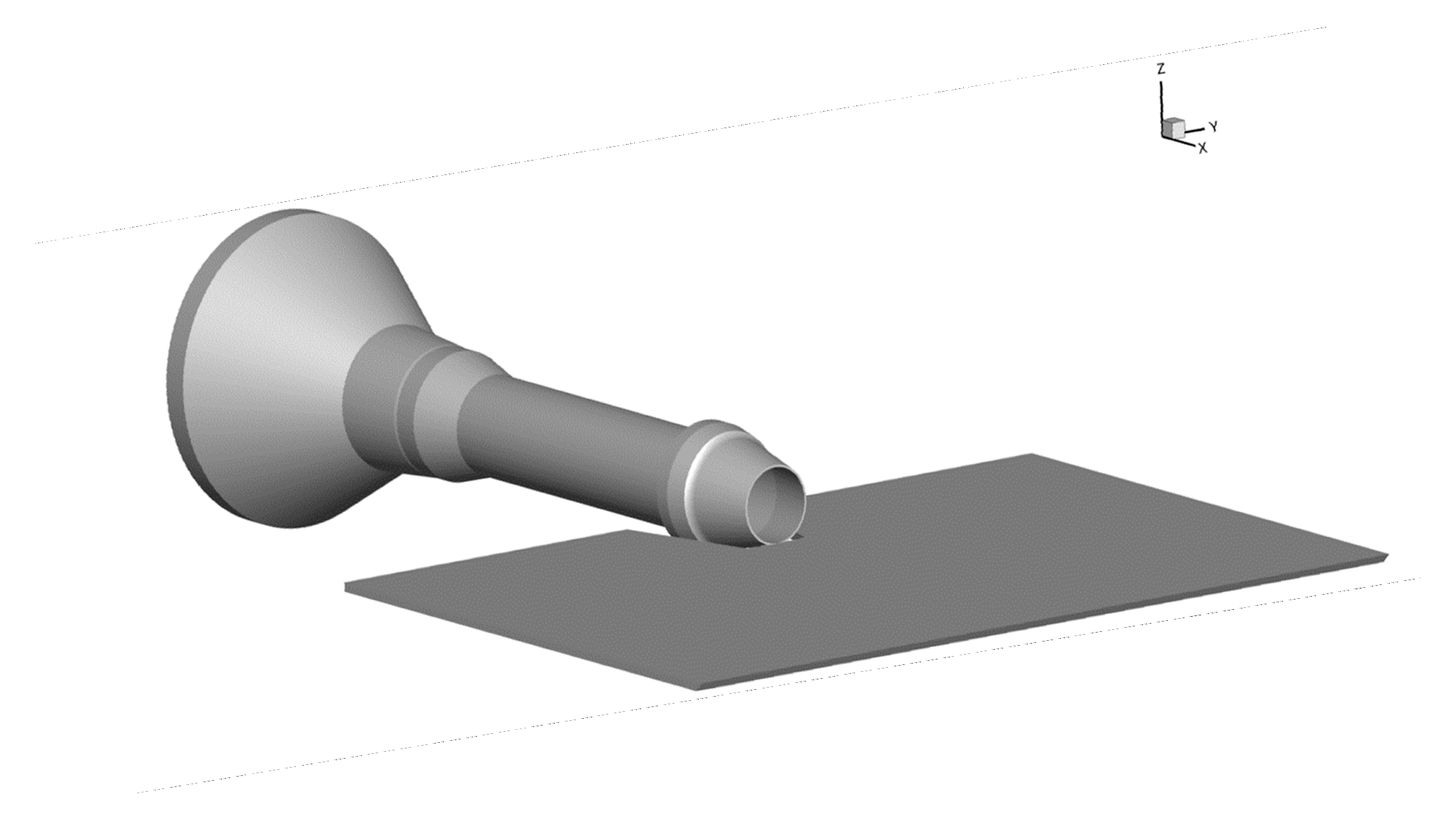
The low-frequency Green’s theory was used to predict the sound field produced by the interaction of circular jet with a trailing edge in [42] (see Figure 5). Their formulas turn out to be quite general and are expected to apply to many different flow configurations, such as the multiple jet configuration shown in Figure 6. They carried out computations over a range of azimuthal angles and three different Mach numbers and again obtained good agreement with experiment. Some typical comparisons are presented in Figure 7.

12. Concluding Remarks

This paper was written to bring together and present in a consistent fashion a general theory for the unsteady motion on a transversely sheared mean flow that has been developed over the years in a number of papers published in the Journal of Fluid Mechanics. The relevant equations are reformulated in terms of a gauge function in order to obtain expressions of the unsteady velocity and pressure fluctuations (which decouple from the entropy fluctuations) that involve two arbitrarily convected quantities. A pair of very general conservation laws are then used to derive upstream boundary conditions that relate two of these quantities to experimentally measurable flow variables.

Inflectional base flows are able to support spatially growing instability waves, which are often associated with the coherent structures in turbulent flows. Their amplitudes cannot be determined by imposing upstream boundary conditions, but can be uniquely determined as part of the solution when causality is imposed on the flow-which appears to be particularly appropriate in the present context since Creighton [24,25] has shown that the imposition of causality is equivalent to imposing a Kutta condition at a trailing edge.

The entropy fluctuations can be determined after the fact once the velocity and pressure fluctuations are known by specifying a third arbitrary quantity. The results, which can be used to analyze the unsteady motion resulting from the interaction of turbulent shear flows with solid surfaces, are applicable to a wide range of flow–surface interaction problems.

References

1. Bilka, M.J.; Kerrian, P.; Ross, M.H.; Morris, S.C. Radiated Sound from a Circular Cylinder in a Turbulent Shear Layer. Int. J. Aeroacoust. 2014, 13, 511–532. [Google Scholar] [CrossRef]
2. Tufts, A.; Wang, K.; Wang, M. Computational study of sound by airfoil interaction with a turbulent shear layer, AIAA paper # 2018-0757. In Proceedings of the AIAA Aerospace Sciences Meeting, Kissimmee, FL, USA, 8–12 January 2018. [Google Scholar]
3. Ross, M.H. Radiated Sound Generated by Airfoils in a Single Stream Shear Layer. Master’s Thesis, University of Notre Dame, Notre Dame, IN, USA, April 2009. [Google Scholar]
4. Hunt, J.C.R. A theory of turbulent flow round two-dimensional bluff bodies. J. Fluid Mech. 1973, 61, 625–706. [Google Scholar] [CrossRef]
5. Goldstein, M.E. Unsteady vortical and entropic distortions of potential flows round arbitrary obstacles. J. Fluid Mech. 1978, 89, 433–468. [Google Scholar] [CrossRef]
6. Goldstein, M.E. Turbulence generated by entropy fluctuation with non-uniform mean flows. J. Fluid Mech. 1979, 93, 209–224. [Google Scholar] [CrossRef]
7. Sagaut, P.; Cambon, C. Homogeneous Turbulence Dynamics; Cambridge University Press: Cambridge, UK, 2008. [Google Scholar]
8. Batchelor, G.K.; Proudman, I. The effect of rapid distortion of a fluid in turbulent motion. Q. J. Mech. Appl. Math. 1954, 7, 83–103. [Google Scholar] [CrossRef]
9. Kovasznay, L.S.G. Turbulence in Supersonic Flow. J. Aeronaut. Sci. 1953, 20, 657–674. [Google Scholar] [CrossRef]
10. Möhring, W. Über Schallwellen in Scherströmungen. In Fortschritte der Akustik—DAGA; VDI: Düsseldorf, Germany, 1976; Volume 76, pp. 543–546. [Google Scholar]
11. Sears, W.R. Some Aspects of Non-Stationary Airfoil Theory and Its Practical Application. J. Aeronaut. Sci. 1941, 8, 104–108. [Google Scholar] [CrossRef]
12. Amiet, R.K. Acoustic radiation from an Airfoil in a turbulent stream. J. Sound Vib. 1975, 81, 407–420. [Google Scholar] [CrossRef]
13. Paterson, R.W.; Amiet, R.K. Acoustic radiation and surface pressure characteristics ofan Airfoil due to incident turbulence, AIAA paper #76-571. In Proceedings of the AIAA Aeroacoustics Conference, Palo Alto, CA, USA, 20–23 July 1976. [Google Scholar]
14. Orr, W. The stability and instability of the steady motions of a perfect liquid and of a viscous liquid. Proc. R. Irish Acad. A 1907, 27, 69–138. [Google Scholar]
15. Drazin, P.G.; Reid, W.H. Hydrodynamic Stability; Cambridge University Press: Cambridge, UK, 1981; pp. 147–151. [Google Scholar]
16. Brinckman, K.W.; Walker, J.D.A. Instability in a viscous flow driven by streamwise vortices. J. Fluid Mech. 2001, 432, 127–166. [Google Scholar] [CrossRef]
17. Cowley, S.J. Laminar Boundary-layer Theory: A 20th Century Paradox? In Proceedings of the 20th International Congress of Theoretical and Applied Mechanics, Chicago, IL, USA, 27 August–2 September 2000; Kluwer: Dordrecht, The Netherlands, 2001; pp. 389–411. [Google Scholar]
18. Cassel, K.W.; Conlisk, A.T. Unsteady separation in vortex-induced boundary layers. Philos. Trans. R. Soc. A Math. Phys. Eng. Sci. 2014, 372, 20130348. [Google Scholar] [CrossRef] [PubMed] [Green Version]
19. Gradshteyn, I.S.; Ryzhik, I.M. Table of Integrals Series and Products; Academic Press: Cambridge, MA, USA, 1965; p. 406. [Google Scholar]
20. Goldstein, M.E.; Leib, S.J.; Afsar, M.Z. Generalized rapid-distortion theory on transversely sheared mean flows with physically realizable upstream boundary conditions: Application to trailing-edge problem. J. Fluid Mech. 2017, 824, 477–512. [Google Scholar] [CrossRef] [Green Version]
21. Goldstein, M.E. Scattering and distortion of the unsteady motion on transversely sheared mean flows. J. Fluid Mech. 1979, 91, 601–632. [Google Scholar] [CrossRef]
22. Xie, Z.; Karimi, M.; Girimaji, S.S. Small perturbation evolution in compressible Poiseulle flow-velocity interactions and obliqueness effects. J. Fluid Mech. 2017, 814, 249–276. [Google Scholar] [CrossRef]
23. Moffatt, H.K. Interaction of turbulence with strong wind Shear. In Proceedings of the Colloquium on Atmospheric Turbulence and Radio Wave Propagation, Moscow, Russia, 15–22 June 1965; Yaglom, A.M., Tatarski, V.I., Eds.; Nauka: Moscow, Russia, 1967; pp. 139–156. [Google Scholar]
24. Ayton, L.J.; Gill, J.; Peake, N. The importance of the unsteady Kutta condition when modelling gust–aerofoil interaction. J. Sound Vib. 2016, 378, 28–37. [Google Scholar] [CrossRef] [Green Version]
25. Crighton, D.G. The Kutta condition in unsteady flow. Ann. Rev. Fluid Mech. 1985, 17, 411–445. [Google Scholar] [CrossRef]
26. Goldstein, M.E. Aeroacoustics; McGraw-Hill Book Company: New York, NY, USA, 1976. [Google Scholar]
27. Goldstein, M.E.; Afsar, M.Z.; Leib, S.J. Non-homogeneous rapid distortion theory on transversely sheared mean flows. J. Fluid Mech. 2013, 736, 532–569. [Google Scholar] [CrossRef]
28. Haurwitz, B. Zur theorie der wellenbewegungen in luft und wasser. Veroff. Geophys. Inst. Leipz. 1931, 6, 324–364. [Google Scholar]
29. Morse, P.M.; Feshbach, H. Methods of Theoretical Physics; McGraw-Hill Book Company: New York, NY, USA, 1953; p. 870. [Google Scholar]
30. Weiner, N. The use of statistical theory to study turbulence. In Proceedings of the Fifth International Congress for Applied Mechanics, Cambridge, MA, USA, 12–16 September 1938; pp. 356–360. [Google Scholar]
31. Tam, C.K.W.; Auriault, L. Mean flow refraction effects on sound radiated from localized sources. J. Fluid Mech. 1998, 370, 149–174. [Google Scholar] [CrossRef]
32. Briggs, R.J. Electron Stream Interaction with Plasmas; MIT Press: Cambridge, MA, USA, 1964. [Google Scholar]
33. Bers, A. Linear waves and instabilities. In Plasma Physics; Dewitt, C., Perraud, J.D., Eds.; Gordon and Breach Science: New York, NY, USA, 1975; pp. 123–216. [Google Scholar]
34. Baker, D.J.; Peake, N. Scattering on rotational flows, Paper # AIAA-2019-2554. In Proceedings of the 25th AIAA/ACEAS Aeroacoustics Conference, Delft, The Netherlands, 20–23 May 2019. [Google Scholar]
35. Noble, B. Methods Based on the Wiener-Hopf Technique for the Solution of Partial Differential Equations; Pergamon: Oxford, UK, 1958. [Google Scholar]
36. Zaman, K.; Brown, C.A.; Bridges, J.E. Interaction of a Rectangular Jet with a Flat-plate placed parallel to the Flow. AIAA-2013-2184. NASA/TM-2013-217879 (E-18684). In Proceedings of the 19th AIAA/CEAS Aeroacoustics Conference, Berlin, Germany, 27–29 May 2013. [Google Scholar]
37. Bridges, J.; Brown, C.A.; Bozak, R. Experiments on Exhaust of Tightly Integrated Propulsion Systems, AIAA-2014-2904. In Proceedings of the 20th AIAA/CEAS Aeroacoustics Conference, Atlanta, GA, USA, 16–20 June 2014. [Google Scholar]
38. Brown, C.A. An Empirical Jet-Surface Interaction Noise Model with Temperature and Nozzle Aspect Ratio Effects. In Proceedings of the 53rd AIAA Aerospace Sciences Meeting, Kissimmee, FL, USA, 5–9 January 2015. [Google Scholar]
39. Brown, C. Jet-Surface Interaction Test: Far-Field Noise Results, ASME Paper GT2012-69639. In Proceedings of the ASME Turbo Expo 2012: Turbine Technical Conference and Exposition, Copenhagen, Denmark, 11–15 June 2012. [Google Scholar]
40. Bridges, J. Noise from Aft Deck Exhaust Nozzles—Differences in Experimental Embodiments. In Proceedings of the 52nd AIAA Aerospace Sciences Meeting, Nat’l Harbor, MD, USA, 13–17 January 2014. [Google Scholar]
41. Goldstein, M.E.; Afsar, M.Z.; Leib, S.J. Structure of Small Amplitude Motion on Transversely Sheared Mean Flows, NASA/TM-2013-217862; National Aeronautics and Space Administration (NASA): Washington, DC, USA, 2013. [Google Scholar]
42. Goldstein, M.E.; Leib, S.J.; Afsar, M.Z. Rapid distortion theory on transversely sheared mean flows of arbitrary cross-section. J. Fluid Mech. 2019, 881, 551–584. [Google Scholar] [CrossRef] [Green Version]
43. Olsen, W.; Boldman, D. Trailing edge noise data with comparison to theory, AIAA Paper # 79-1524. In Proceedings of the AIAA 12th Fluid and Plasma Dynamics Conference, Williamsburg, VA, USA, 23–25 July 1979. [Google Scholar]
44. Ayton, L.J.; Peake, N. An analytic approach to high-frequency gust-airfoil interaction noise in steady shear flows, Paper # AIAA-2014-2322. In Proceedings of the 20th AIAA/CEAS Aeroacoustics Conference, Atlanta, GA, USA, 16–20 June 2014. [Google Scholar]
45. Baker, D.I.; Peake, N. Effect of boundary-layer shear on trailing edge noise. Paper # AIAA-2017-3169. In Proceedings of the 23rd AIAA/CEAS Aeroacoustics Conference, Denver, CO, USA, 5–9 June 2017. [Google Scholar]
46. Afsar, M.Z.; Leib, S.; Bozak, R. Effect of de-correlating turbulence on the low frequency decay of jet-surface interaction noise in sub-sonic unheated air jets using a CFD-based approach. J. Sound Vib. 2017, 386, 177–207. [Google Scholar] [CrossRef] [Green Version]
47. Khavaran, A.; Bozak, R.F.; Brown, C.A. Jet Surface Interaction Noise in a Planar Exhaust, AIAA-2016-2863. In Proceedings of the 22nd AIAA/CEAS Aeroacoustics Conference, Lyon, France, 30 May–1 June 2016. [Google Scholar]
48. Ramakrishnan, K.; Paliath, U.; Pastouchencko, N.; Malcevic, I.; Pilon, A.; Morgenstern, J.; Buonanno, M.; Martinez, M.; Majjigi, M. Evaluation of Low Noise Integration Concepts and Propulsion Technologies for Future Supersonic Civil Transports; NASA CR-2018-219936; National Aeronautics and Space Administration (NASA): Washington, DC, USA, 2018. [Google Scholar]
49. Williams, J.E.F.; Hall, L.H. Aerodynamic sound generation by turbulent flow in the vicinity of a scattering half plane. J. Fluid Mech. 1970, 40, 657–670. [Google Scholar] [CrossRef]
50. Pope, S. Turbulent Flows, 1st ed.; Cambridge University Press: Cambridge, UK, 2000. [Google Scholar]
51. Leib, S.J.; Goldstein, M.E. Hybrid Source Model for Predicting High-Speed Jet Noise. AIAA J. 2011, 49, 1324–1335. [Google Scholar] [CrossRef]
52. Campbell, G.A.; Foster, R.M. Fourier Integrals for Practical Applications; D. Van Nostrand Co. Inc.: Princeton, NJ, USA, 1948; p. 111. [Google Scholar]
Figure 1. Transverse velocity fluctuations produced by the convected vorticity given by Equations (9) and (10) for the indicated values of the parameters. (a) Real part; (b) imaginary part. Reproduced with permission from [20].
Fluids 05 00062 g001aFluids 05 00062 g001b
Figure 2. Leading edge scattering. Reproduced with permission from [20].
Fluids 05 00062 g002
Figure 3. Rectangular jet interacting with the trailing edge of a flat plate.
Fluids 05 00062 g003
Figure 4. Comparisons of theoretically predicted power spectral density (PSD), at various Strouhal numbers for a planar jet with experimental data of Brown [30] at an Acoustic Mach number of 0.9 based on the jet exit velocity and equivalent nozzle diameter at polar angles (a) θ = 95 ° and (b) θ = 105 ° . Reproduced with permission from [20].
Fluids 05 00062 g004
Figure 5. Round jet interacting with the trailing edge of a flat plate.
Fluids 05 00062 g005
Figure 6. Supersonic cruise concept aircraft with top mounted engines. Reproduced with permission from Ramakrishnan et al. NASA CR-2018-219936 [48] (provided by Dr. James Bridges).
Fluids 05 00062 g006
Figure 7. Comparison of composite round jet Rapid Distortion Theory (RDT) solution with the power spectral density (PSD) of the far-field pressure fluctuation vs. Strouhal number, St, based on jet exit velocity and nozzle diameter at polar angles: (a) θ = 75 ° and (b) θ = 105 ° measured from the downstream jet axis by Brown [38,39]. The acoustic Mach number based on jet exit velocity is equal to 0.9. Reproduced with permission from [42].
Fluids 05 00062 g007