Approximating Isoneutral Ocean Transport via the Temporal Residual Mean

Abstract

Ocean volume and tracer transports are commonly computed on density surfaces because doing so approximates the semi-Lagrangian mean advective transport. The resulting density-averaged transport can be related approximately to Eulerian-averaged quantities via the Temporal Residual Mean (TRM), valid in the limit of small isopycnal height fluctuations. This article builds on a formulation of the TRM for volume fluxes within Neutral Density surfaces, (the “NDTRM”), selected because Neutral Density surfaces are constructed to be as neutral as possible while still forming well-defined surfaces. This article derives a TRM, referred to as the “Neutral TRM” (NTRM), that approximates volume fluxes within surfaces whose vertical fluctuations are defined directly by the neutral relation. The purpose of the NTRM is to more closely approximate the semi-Lagrangian mean transport than the NDTRM, because the latter introduces errors associated with differences between the instantaneous state of the modeled/observed ocean and the reference climatology used to assign the Neutral Density variable. It is shown that the NDTRM collapses to the NTRM in the limiting case of a Neutral Density variable defined with reference to the Eulerian-mean salinity, potential temperature and pressure, rather than an external reference climatology, and therefore that the NTRM approximately advects this density variable. This prediction is verified directly using output from an idealized eddy-resolving numerical model. The NTRM therefore offers an efficient and accurate estimate of modeled semi-Lagrangian mean transports without reference to an external reference climatology, but requires that a Neutral Density variable be computed once from the model’s time-mean state in order to estimate isopycnal and diapycnal components of the transport.

1. Introduction

Accurate quantification of the ocean’s meridional overturning circulation (MOC) is required to infer oceanic transport of heat and other tracers around the globe [1,2]. It has been common practice for decades to quantify the MOC in some form of density coordinate system (e.g., [3,4,5,6,7,8]). Because flow in the ocean interior is quasi-adiabatic, this approach approximately corresponds to taking a semi-Lagrangian mean, which in turn approximates the full Lagrangian-mean transport [9]. In comparison to an MOC based on mass fluxes averaged at constant depth, the semi-Lagrangian mean transport velocity contains an additional “eddy” transport, essentially a generalized Stokes drift [10]. This eddy transport is particularly important in the Southern Ocean [11,12,13], and therefore forms a key component of recent conceptual models of the global overturning circulation [14,15,16,17,18,19].

The separation of the semi-Lagrangian mean transport into mean and eddy components can be made explicit via the Temporal Residual Mean (TRM) formulation, which is valid in the asymptotic limit of small isopycnal height fluctuations [9,20,21]. In this article we use “TRM” to refer to the TRM-II [21], but it is straightforward to extend our results to the TRM-I; the distinction between the two is discussed by [22]. The TRM relates the eddy component of the transport to correlations between the lateral velocity ($\mathit{u}$) and density ($\gamma$) fields, and thereby allows an estimate of the semi-Lagrangian mean transport streamfunction to be computed from Eulerian-averaged quantities. The resulting TRM streamfunction $\mathsf{\Psi }$ advects the density variable $\gamma$ in the following sense: in the absence of non-conservative sources and sinks of $\gamma$, the density $\gamma$ is materially conserved following the transport velocity defined by $\mathsf{\Psi }$, up to a consistent asymptotic order in the amplitude of the isopycnal height fluctuations [22].

This article builds upon the Neutral Density Temporal Residual Mean (NDTRM) formulation ([23], [hereafter ST15]). In ST15’s formulation the Neutral Density variable of [24], referred to henceforth as ${\gamma }^{\mathrm{JM}97}$, was the advected density variable. However, the transport streamfunction $\mathsf{\Psi }$ was calculated from correlations between the lateral velocity, salinity, potential temperature and pressure. This approach bears the following advantages: (i) The NDTRM can be applied in regions where potential density referenced to any level becomes vertically non-monotonic somewhere in the water column (e.g., parts of the high-latitude oceans). (ii) The NDTRM circumvents the computational expense of calculating Neutral Density globally at every model time step, as would be required to compute the semi-Lagrangian mean transport velocity, either exactly or via the TRM. (iii) More fundamentally, isopycnals of Neutral Density are more closely aligned with the local neutral tangent plane, in a global sense, than any potential density variable [24]. ST15 compared various formulations of the TRM, and verified that higher-order approximations to the NDTRM most closely approximated the volume fluxes computed exactly within ${\gamma }^{\mathrm{JM}97}$ surfaces from numerical model output. The NDTRM therefore offers a computationally efficient estimate of isopycnal volume fluxes within surfaces of a stably stratified density variable that has been used widely in quantifications of the ocean’s global overturning circulation (e.g., [5,25]).

In this article we pursue the related but distinct goal of approximating the semi-Lagrangian mean transport using vertical fluctuations defined directly by the neutral relationship [26], which we refer to as local Neutral Surfaces. In pursing this goal we make the assumption that it is these local Neutral Surfaces that should heave vertically under perfectly adiabatic motions [27,28], and therefore that they are best suited for calculation of the semi-Lagrangian mean transport [9]. The validity of these assumptions is discussed further in Section 5. In Section 2 we summarize relevant background literature, specifically the formulation of the TRM [20,21] and the derivation of the NDTRM by ST15. In Section 3 we derive a form of the TRM, which we refer to as the “Neutral TRM” (NTRM), that approximates volume fluxes within local Neutral Surfaces. However, Neutral Surfaces are globally ill-defined [29]. This means that isoneutral volume fluxes cannot be associated with a globally-defined, stably-stratified density variable [30], which is desireable for quantifying global circulation and water mass transformation [5,25,31]. This motivates us to return to the NDTRM, which is associated with a globally-defined density variable, and consider the special case of a Neutral Density constructed with reference to the Eulerian-mean salinity, potential temperature and pressure. We show that in this case, the NDTRM reduces to the NTRM to a consistent asymptotic order in the amplitude of the isopycnal height fluctuations. This implies that the NTRM advects a Neutral Density variable defined with respect to the Eulerian-mean ocean state, again up to a consistent asymptotic order in the amplitude of the isopycnal height fluctuations. In Section 4 we evaluate our results using idealized numerical simulations, and verify that the NTRM and NDTRM more closely approximate volume fluxes within Neutral Density surfaces constructed based on the model’s mean state and based on an independent reference dataset, respectively. Finally, in Section 5 we summarize and provide concluding remarks.

2. Approximating Volume Fluxes within Neutral Density Surfaces

There is a substantial existing literature on the subjects of Neutral Surfaces and the TRM approximation (e.g., [20,21,24,26]). To achieve a self-contained presentation, this section summarizes relevant concepts from this literature, and from the derivation of the NDTRM by ST15.

2.1. The Temporal Residual Mean (TRM) Streamfunction

The TRM transport is fundamentally related to fluctuations of material or quasi-material surfaces, typically defined in terms of a density/buoyancy variable [20,21]. While it is impractical to quantify the Lagrangian-mean transport of fluid parcels in the ocean in the most general sense [32], a close approximation can be obtained by exploiting vertically stratified, quasi-material surfaces, commonly defined via a suitable density or buoyancy variable [22]. Consider a series of vertically monotonic, temporally-evolving, quasi-material surfaces identified by a label ${\gamma }_0$, currently not assigned any physical meaning. We define a streamfunction $\mathsf{\Psi }$ at any horizontal point $(x_0,y_0)$ on surface ${\gamma }_0$ as the lateral mass flux above that surface,

$$\mathsf{\Psi }(x_0,y_0,{\gamma }_0)=\overline{{\int }_{z=z_0(x_0,y_0,{\gamma }_0,t)}^{z=0}\mathit{u}\mathrm{d}z},$$

(1)

where $\mathit{u}=(u,v)$ is the horizontal velocity vector and we have assumed a flat ocean surface ($z=0$) for simplicity. The overline indicates a time average, but could be interpreted more broadly as an average over an ensemble of realizations of the flow [33].

The TRM approximates the mass flux defined in (1) under the assumption of small fluctuations in the quasi-material surfaces, i.e., $z_0=\overline{z_0}+z_0^{\prime }$ with $z_0^{\prime }=\mathcal{O}\left(\epsilon \right)$ assumed to be asymptotically small. Here $\epsilon$ may be interpreted as the magnitude of the surface fluctuation relative to some vertical length scale such as the ocean depth H, so $\epsilon =z_0^{\prime }/H\ll 1$. Using Taylor expansions of (1), it may be shown (e.g., [21,23]) that $\mathsf{\Psi }$ may be approximated in Eulerian coordinates as a sum of mean and “eddy” components, defined as

$$\begin{array}{cc}\hfill \mathsf{\Psi }(x_0,y_0,\overline{z_0})& =\overline{\mathsf{\Psi }}+{\mathsf{\Psi }}^{\star },\hfill \end{array}$$

(2)

$$\begin{array}{cc}\hfill \overline{\mathsf{\Psi }}& ={\int }_{\overline{z_0}}^0\overline{\mathit{u}}\mathrm{d}z,\hfill \end{array}$$

(3)

$$\begin{array}{cc}\hfill {\mathsf{\Psi }}^{\star }& =-\overline{{\mathit{u}}^{\prime }\left(\overline{z_0}\right)z_0^{\prime }}-\frac{1}{2}{\overline{\mathit{u}}}_z\left(\overline{z_0}\right)\overline{{z_0^{\prime }}^2}+\mathcal{O}\left({\epsilon }^3\right).\hfill \end{array}$$

(4)

Here, and henceforth in this manuscript, the rules of Reynolds averaging are assumed to apply unless otherwise stated, i.e., $\overline{\overline{•}}=\overline{•}$ and $\overline{{•}^{\prime }}=0$ for any •. Note that $\overline{\mathsf{\Psi }}$ and ${\mathsf{\Psi }}^{\star }$ are streamfunctions in the sense that their curl is equal to a non-divergent velocity field.

To write (2) in terms of only mean quantities, and therefore to create a useful approximation to the ocean’s Lagrangian-mean velocities, we require a suitable approximation to the surface fluctuations $z_0^{\prime }$. Correlations of quantities such as $\overline{{\mathit{u}}^{\prime }{z}_0^{\prime }}$ and $\overline{{z_0^{\prime }}^2}$ are not routinely provided as output from ocean models formulated in Eulerian vertical coordinate systems, partly due to the ambiguity in the definition of $z_0$, so instead $z_0^{\prime }$ is typically related to Eulerian fluctuations of thermodynamic variables (e.g., [22,23]). For a vertically monotonic label $\gamma$, we can further Taylor-expand our continuum of labels $\gamma$ to obtain an $\mathcal{O}\left({\epsilon }^2\right)$ approximation to $z_0^{\prime }$ [21,22],

$${\gamma }^{\prime }\left(\overline{z_0}\right)=-z_0^{\prime }{\overline{\gamma }}_z\left(\overline{z_0}\right)+\mathcal{O}\left({\epsilon }^2\right),$$

(5)

allowing us to express the TRM “eddy” streamfunction in terms of purely Eulerian variables,

$${\mathsf{\Psi }}^{\star }(x_0,y_0,\overline{z_0})=\frac{\overline{{\mathit{u}}^{\prime }{\gamma }^{\prime }}}{{\overline{\gamma }}_z}-\frac{1}{2}\frac{{\overline{\mathit{u}}}_z}{{\overline{\gamma }}_z^2}\overline{{{\gamma }^{\prime }}^2}+\mathcal{O}\left({\epsilon }^3\right).$$

(6)

Note that all variables on the right-hand side are evaluated at the mean surface elevation $\overline{z_0}$. Additionally, note that the $\mathcal{O}({\epsilon }^3)$ error terms on the right-hand side of (6) differ from those on the right-hand side of (4); additional $\mathcal{O}({\epsilon }^3)$ terms have been included in the error term following the substitution for ${\gamma }^{\prime }$ using (5). In the interst of brevity, throughout this article we will write the error terms in terms of their lowest-order dependence on the relevant asymptotically small parameters without specifically identifying when the mathematical definition of the error terms has changed.

In the form of equation (6), the TRM streamfunction is in principle straightforward to calculate from ocean model output if we associate $\gamma$ with, for example, potential density or Neutral Density ([24], discussed in Section 2.2). However, potential density surfaces are not particularly neutral, while the Neutral Density variable of [24] is too computationally expensive for practical use in ocean models [23].

2.2. The Neutral Density Temporal Residual Mean (NDTRM)

ST15 derived alternative expressions to (5) for the vertical fluctuations ($z_0^{\prime }$) of isopycnals of a Neutral Density variable ($\gamma$). These expressions contain no explicit dependence on $\gamma$ itself, and so circumvent the need to explicitly compute a Neutral Density variable in order to construct the TRM. Here we briefly summarize the portions of this derivation and the resulting expressions for $z_0^{\prime }$ required in Section 3.

The Neutral Density variable of [24] is assigned based on geographically distributed reference casts. Each reference cast is pre-labeled with Neutral Density $\gamma$ as a function of depth, such that the cast potential temperature, salinity and pressure may be written as ${\theta }_c\left(\gamma \right)$, $S_c\left(\gamma \right)$ and $p_c\left(\gamma \right)$, respectively. To assign a Neutral Density label to a given point in space and time, the potential temperature (${\theta }_0$), salinity ($S_0$) and pressure ($p_0$) at that point are compared with a nearby reference cast. Specifically, the assigned value of $\gamma$ is that which satisfies the “discrete neutral relation”, which ST15 wrote as

$$\begin{array}{c}\left(S_c\left(\gamma \right)-S_0\right){\beta }_m-\left({\theta }_c\left(\gamma \right)-{\theta }_0\right){\alpha }_m=\mathcal{O}\left({\Delta }^3\right).\end{array}$$

(7)

This relation states that water parcels with properties $(S_0,{\theta }_0,p_0)$ and $(S_c\left(\gamma \right),{\theta }_c\left(\gamma \right),p_c\left(\gamma \right))$ would have equal densities if both were moved adiabatically and isentropically to the mid-point pressure between the two parcels. Here ${\beta }_m$ and ${\alpha }_m$ are short-hands for

$${\beta }_m\equiv \beta (S_m,{\theta }_m,p_m),{\alpha }_m\equiv \alpha (S_m,{\theta }_m,p_m),$$

(8)

i.e., the saline contraction and thermal expansion coefficients evaluated at the thermodynamic mid-point $(S_m,{\theta }_m,p_m)$, which is defined as

$$\begin{array}{c}{S}_m\left(\gamma \right)\equiv (S_0+S_c\left(\gamma \right))/2,\end{array}$$

(9)

$$\begin{array}{c}{\theta }_m\left(\gamma \right)\equiv ({\theta }_0+{\theta }_c\left(\gamma \right))/2,\end{array}$$

(10)

$$\begin{array}{c}{p}_m\left(\gamma \right)\equiv (p_0+p_c\left(\gamma \right))/2.\end{array}$$

(11)

The small parameter $\Delta$ measures deviations of the properties $(S_0,{\theta }_0,p_0)$ from the mid-values $(S_m,{\theta }_m,p_m)$. See [23] for further details on the definition of $\Delta$ and the asymptotic derivation of (7).

To derive an expression for the vertical fluctuations of a Neutral Density surface, ST15 considered the semi-Lagrangian evolution of the thermodynamic properties on such a surface, i.e., $S_0=S(z_0\left(t\right),t)$, ${\theta }_0=\theta (z_0\left(t\right),t)$, and $p_0=p(z_0\left(t\right),t)$. They then posed Taylor expansions of (7) in terms of $\epsilon$ and $\Delta$, e.g.,

$$S(z_0\left(t\right),t)=\overline{S(\overline{z_0},t)}+\overline{S_z(\overline{z_0},t)}{z}_0^{\prime }+S^{\prime }(\overline{z_0},t)+\mathcal{O}\left({\epsilon }^2\right).$$

(12)

where $S^{\prime }(\overline{z_0},t)=S(\overline{z_0},t)-\overline{S(\overline{z_0},t)}$ is the Eulerian fluctuation of the salinity at $z=\overline{z_0}$.

In this article we restrict our attention to the Boussinesq case for simplicity. This effectively corresponds to replacing $p_0$, $p_c$ and $p_m$ by $z_0$, $z_c$ and $z_m$, where $z_c$ is the depth of the Neutral Density label $\gamma$ on the reference cast and $z_m=\frac{1}{2}(z_0+z_c)$. In this case, the highest-order NDTRM approximation to $z_0^{\prime }$ (the “NDTRM2” of ST15) is

$$\begin{array}{c}{z}_{\mathrm{NDTRM}2}^{\prime }\left\{-{\overline{S}}_z{\widehat{\beta }}_m+{\overline{\theta }}_z{\widehat{\alpha }}_m\right.+\left(S_c-\overline{S}\right)\left[\frac{1}{2}{\overline{S}}_z\frac{\partial {\widehat{\beta }}_m}{\partial \overline{S_m}}+\frac{1}{2}{\overline{\theta }}_z\frac{\partial {\widehat{\beta }}_m}{\partial \overline{{\theta }_m}}+\frac{1}{2}\frac{\partial {\widehat{\beta }}_m}{\partial \overline{z_m}}\right]\hfill \\ \left.-\left({\theta }_c-\overline{\theta }\right)\left[\frac{1}{2}{\overline{S}}_z\frac{\partial {\widehat{\alpha }}_m}{\partial \overline{S_m}}+\frac{1}{2}{\overline{\theta }}_z\frac{\partial {\widehat{\alpha }}_m}{\partial \overline{{\theta }_m}}+\frac{1}{2}\frac{\partial {\widehat{\alpha }}_m}{\partial \overline{z_m}}\right]\right\}\\ =-\left\{-S^{\prime }{\widehat{\beta }}_m+{\theta }^{\prime }{\widehat{\alpha }}_m+\left(S_c-\overline{S}\right)\left[\frac{1}{2}{S}^{\prime }\frac{\partial {\widehat{\beta }}_m}{\partial \overline{S_m}}+\frac{1}{2}{\theta }^{\prime }\frac{\partial {\widehat{\beta }}_m}{\partial \overline{{\theta }_m}}\right]-\left({\theta }_c-\overline{\theta }\right)\left[\frac{1}{2}{S}^{\prime }\frac{\partial {\widehat{\alpha }}_m}{\partial \overline{S_m}}+\frac{1}{2}{\theta }^{\prime }\frac{\partial {\widehat{\alpha }}_m}{\partial \overline{{\theta }_m}}\right]\right\}\\ \hfill +\mathcal{O}\left({\Delta }^3,{\epsilon }^2\right).\end{array}$$

(13)

Here we use shorthand notation for the Eulerian-mean salinity and potential temperature at constant height,

$$\overline{S}\left(\overline{z_0}\right)\equiv \overline{S(\overline{z_0},t)},\overline{\theta }\left(\overline{z_0}\right)\equiv \overline{\theta (\overline{z_0},t)},$$

(14)

and for the haline contraction and thermal expansion coefficients evaluated as functions of Eulerian-mean properties,

$${\widehat{\beta }}_m\equiv \beta \left(\overline{S_m},\overline{{\theta }_m},\overline{z_m}\right),{\widehat{\alpha }}_m\equiv \alpha \left(\overline{S_m},\overline{{\theta }_m},\overline{z_m}\right).$$

(15)

Equation (13) approximately relates the Neutral Surface height fluctuations to Eulerian fluctuations of S and $\theta$, in analogy with (5). By excluding terms from (13), ST15 derived lower-order approximations to $z_0^{\prime }$, referred to as the “NDTRM1”,

$$z_{\mathrm{NDTRM}1}^{\prime }=-\frac{S^{\prime }{\widehat{\beta }}_m-{\theta }^{\prime }{\widehat{\alpha }}_m}{{\overline{S}}_z{\widehat{\beta }}_m-{\overline{\theta }}_z{\widehat{\alpha }}_m}+\mathcal{O}\left({\Delta }^3,{\epsilon }^2,\epsilon \tilde{\Delta }\right),$$

(16)

and “NDTRM0”

$$z_{\mathrm{NDTRM}0}^{\prime }=-\frac{S^{\prime }\widehat{\beta }-{\theta }^{\prime }\widehat{\alpha }}{{\overline{S}}_z\widehat{\beta }-{\overline{\theta }}_z\widehat{\alpha }}+\mathcal{O}\left({\Delta }^3,{\tilde{\Delta }}^2,{\epsilon }^2,\epsilon \tilde{\Delta }\right),$$

(17)

where we define

$$\widehat{\beta }\equiv \beta \left(\overline{S},\overline{\theta },\overline{z_0}\right),\widehat{\alpha }\equiv \alpha \left(\overline{S},\overline{\theta },\overline{z_0}\right),$$

(18)

in analogy with (15). For brevity we omit complete expressions for the NDTRM streamfunctions, derived by substituting (13)–(17) into (2), and a discussion of the evaluation of the “cast” terms $S_c$ and ${\theta }_c$; we refer the reader to ST15 for information on such specifics of the NDTRM.

These expressions differ from those given by ST15 via the introduction of an additional small parameter, $\tilde{\Delta }$, that measures deviations of the Eulerian mean properties, $\overline{S}$ and $\overline{\theta }$, from the cast properties, $S_c$ and ${\theta }_c$. Thus, conceptually, the three small parameters in (13)–(17) are related via $\Delta \sim \tilde{\Delta }+\epsilon$.

3. Approximating Volume Fluxes within Local Neutral Surfaces

The Neutral Density variable of [24] (${\gamma }^{\mathrm{JM}97}$) was formulated with the aim of obtaining a density-like variable whose surfaces lie as parallel as possible to the local neutral tangent plane everywhere in the ocean. However, due to the ocean’s equation of state, is not possible to construct such a variable exactly [29,30]. Thus in general the vertical fluctuations of Neutral Density surfaces differ from from fluctuations of local Neutral Surfaces [34]. In Section 1 we posited that local Neutral Surfaces are best suited to estimating semi-Lagrangian mean transport, and therefore also to formulating the TRM, because adiabatic flows are constrained to follow these surfaces. The validity of these assumptions is discussed further in Section 5.

In this section we aim to formulate a TRM that approximates fluxes along local Neutral Surfaces as closely as possible (the NTRM). We first derive an approximation to the vertical fluctuations of local Neutral Surfaces, denoted $z_{\mathrm{NS}}^{\prime }$, for comparison with the NDTRM approximations to $z_0^{\prime }$ given in Section 2. This approximation alone yields an incomplete TRM because the resulting streamfunction (2) is not associated with a globally-defined set of surfaces (i.e., $\gamma$). To circumvent this issue we consider a Neutral Density variable ${\gamma }^{\mathrm{mean}}$ whose reference dataset (i.e., $S_c$, ${\theta }_c$ and $p_c$) is chosen to be the local Eulerian-mean thermodynamic properties (i.e., $\overline{S}$, $\overline{\theta }$ and $\overline{z}$). For such a Neutral Density variable the NDTRM reduces to the NTRM, up to the same asymptotic order in $\epsilon$, which implies that the NTRM does in fact advect a globally-defined density variable, ${\gamma }^{\mathrm{mean}}$. We also show that the NTRM coincides with a TRM derived based on fluctuations of surfaces of locally-referenced potential density, up to the same asymptotic order in $\epsilon$.

3.1. Vertical Fluctuations of Local Neutral Surfaces

Consider a local Neutral Surface with instantaneous height $z=z_0\left(t\right)$ at a fixed horizontal location $(x_0,y_0)$. To simplify our presentation we will drop all dependence on horizontal location in what follows. We define the time-evolution of $z_0\left(t\right)$ via the semi-Lagrangian neutral relationship [26],

$$\beta \delta S(z_0\left(t\right),t)-\alpha \delta \theta (z_0\left(t\right),t)=0,$$

(19)

where $\delta S$ and $\delta \theta$ denote infinitesimal changes in the salinity and potential temperature on the surface. Both $\beta$ and $\alpha$ are themselves evaluated at the local salinity $S(z_0\left(t\right),t)$, potential temperature $\theta (z_0\left(t\right),t)$ and pressure $p(z_0\left(t\right),t)$. Dividing by an infinitesimal unit of time $\delta t$, Equation (19) may be expanded to describe the time evolution of $z_0$,

$$\left[\beta \frac{\partial S}{\partial z}(z_0,t)-\alpha \frac{\partial \theta }{\partial z}(z_0,t)\right]\frac{\mathrm{d}{z}_0}{\mathrm{d}t}=-\left[\beta \frac{\partial S}{\partial t}(z_0,t)-\alpha \frac{\partial \theta }{\partial t}(z_0,t)\right].$$

(20)

We now use (20) to derive a relationship between the Neutral Surface height fluctuations $z_0^{\prime }=z_0\left(t\right)-\overline{z_0}$ and the Eulerian fluctuations of S and $\theta$. Note that fluctuations of S and $\theta$ may not only be associated with vertical heaving of Neutral Surfaces; they may also result from lateral stirring of property gradients along Neutral Surfaces. To simplify the presentation we assume that the magnitudes of both vertical heaving-induced and lateral stirring-induced property fluctuations are small and characterized by the same small parameter $\epsilon$. A caveat to this assumption is that even outside of the ocean’s surface and bottom boundary layers there may be a non-negligible influence of surface buoyancy fluxes [35]. For further discussion of these points and a rationalization of the small parameter $\epsilon$, the reader is referred to ST15.

By posing Taylor expansions of $\beta$ and $\alpha$ as e.g.,

$$\beta \left(S(z_0\left(t\right),t),\theta (z_0\left(t\right),t),z_0\left(t\right)\right)=\beta \left(\overline{S}\left(\overline{z_0}\right),\overline{\theta }\left(\overline{z_0}\right),\overline{z_0}\right)+\mathcal{O}\left(\epsilon \right)=\widehat{\beta }+\mathcal{O}\left(\epsilon \right),$$

(21)

we can approximate (20) as

$$\left[\widehat{\beta }\overline{\frac{\partial S}{\partial z}(\overline{z_0},t)}-\widehat{\alpha }\overline{\frac{\partial \theta }{\partial z}(\overline{z_0},t)}\right]\frac{\mathrm{d}{z}_0^{\prime }}{\mathrm{d}t}=-\left[\widehat{\beta }\frac{\partial S^{\prime }}{\partial t}(\overline{z_0},t)-\widehat{\alpha }\frac{\partial {\theta }^{\prime }}{\partial t}(\overline{z_0},t)\right]+\mathcal{O}\left({\epsilon }^2\right).$$

(22)

Finally, integrating (22) with respect to t yields an expression for the local Neutral Surface height fluctuation, which we denote as $z_{\mathrm{NS}}^{\prime }$, in terms of $S^{\prime }$ and ${\theta }^{\prime }$,

$$\left(\widehat{\beta }\frac{\partial \overline{S}}{\partial \overline{z_0}}-\widehat{\alpha }\frac{\partial \overline{\theta }}{\partial \overline{z_0}}\right)z_{\mathrm{NS}}^{\prime }=-\left(\widehat{\beta }{S}^{\prime }-\widehat{\alpha }{\theta }^{\prime }\right)+\mathcal{O}\left({\epsilon }^2\right).$$

(23)

Note that the constant of integration vanishes between (22) and (23) because by definition, $\overline{z_0^{\prime }}=\overline{S^{\prime }}=\overline{{\theta }^{\prime }}=0$. Substituting (23) into (2)–(4) yields the following expression for the NTRM streamfunction,

$$\mathsf{\Psi }(x_0,y_0,\overline{z_0})={\int }_{\overline{z_0}}^0\overline{\mathit{u}}\mathrm{d}z+\frac{\widehat{\beta }\overline{{\mathit{u}}^{\prime }{S}^{\prime }}-\widehat{\alpha }\overline{{\mathit{u}}^{\prime }{\theta }^{\prime }}}{\widehat{\beta }{\partial }_{\overline{z_0}}\overline{S}-\widehat{\alpha }{\partial }_{\overline{z_0}}\overline{\theta }}-\frac{1}{2}\frac{{\overline{\mathit{u}}}_z\left(\overline{z_0}\right)}{{\left(\widehat{\beta }{\partial }_{\overline{z_0}}\overline{S}-\widehat{\alpha }{\partial }_{\overline{z_0}}\overline{\theta }\right)}^2}\left(\widehat{\beta }{}^2\overline{{S^{\prime }}^2}-2\widehat{\beta }\widehat{\alpha }\overline{S^{\prime }{\theta }^{\prime }}+{\widehat{\alpha }}^2\overline{{{\theta }^{\prime }}^2}\right)+\mathcal{O}\left({\epsilon }^3\right).$$

(24)

Note that in applying (24) we are free to select $\overline{z_0}$, for example to coincide with a model vertical grid level. Equation (23) then approximates the vertical fluctuations of a local Neutral Surface $z_0\left(t\right)$ whose mean elevation is $\overline{z_0}$, and (24) approximates the transport above $z=\overline{z_0}$.

3.2. Connection to the Neutral Density Temporal Residual Mean (NDTRM)

While the NTRM streamfunction (24) approximates the semi-Lagrangian mean transport, in isolation it does not quantify isopycnal/diapycnal fluxes because we have not yet associated it with a globally-defined set of surfaces (i.e., $\gamma$). It therefore does not advect a density variable, and the fluxes cannot be partitioned into adiabatic and diabatic components (e.g., [22]). We therefore now consider whether the NDTRM, which is associated with a globally-defined density variable (e.g., ${\gamma }^{\mathrm{JM}97}$), can be adapted to more closely approximate the fluxes within local Neutral Surfaces.

We first note that there is a close similarity between our equations for the vertical fluctuations of local Neutral Surfaces, (23), and the vertical fluctuations of Neutral Density surfaces, (13)–(17). Indeed, (23) is identical to the lowest-order form of the NDTRM, the NDTRM0 (17), except for the differing asymptotic order of the error terms,

$$z_{\mathrm{NDTRM}0}^{\prime }=z_{\mathrm{NS}}^{\prime }+\mathcal{O}\left({\Delta }^3,{\tilde{\Delta }}^2,\epsilon \tilde{\Delta },{\epsilon }^2\right).$$

(25)

In other words, there are $\mathcal{O}({\Delta }^3)$, $\mathcal{O}({\tilde{\Delta }}^2)$ and $\mathcal{O}(\epsilon \tilde{\Delta })$ terms that appear explicitly on the right-hand sides of (13) and (16), and these terms allow $z_{\mathrm{NDTRM}2}^{\prime }$ and $z_{\mathrm{NDTRM}1}^{\prime }$ to more closely approximate Neutral Density surface fluctuations than $z_{\mathrm{NDTRM}0}^{\prime }$. However, by treating these $\mathcal{O}({\Delta }^3)$, $\mathcal{O}({\tilde{\Delta }}^2)$ and $\mathcal{O}(\epsilon \tilde{\Delta })$ terms as error terms in (17) we actually obtain a closer approximation of local Neutral Surface fluctuations (i.e., of (23)).

Motivated by this observation, we now seek a hypothetical Neutral Density variable that eliminates the $\mathcal{O}({\Delta }^2)$, $\mathcal{O}({\tilde{\Delta }}^2)$ and $\mathcal{O}(\epsilon \tilde{\Delta })$ terms in the NDTRM. This is achieved by constructing a Neutral Density variable, referred to as ${\gamma }^{\mathrm{mean}}$, using the Eulerian-mean thermodynamic properties in place of the reference dataset,

$$(S_c\left(\gamma \right),{\theta }_c\left(\gamma \right),z_c\left(\gamma \right))\to \left(\overline{S}\left(z_r\left(\gamma \right)\right),\overline{\theta }\left(z_r\left(\gamma \right)\right),z_r\left(\gamma \right)\right).$$

(26)

Here we have implicitly assumed that the local water column has been pre-labeled with $\gamma$ based on the Eulerian-mean thermodynamic properties, and the reference elevation $z_r\left(\gamma \right)$ is the elevation in this water column that has been labeled with Neutral Density $\gamma$. The isopycnal fluctuation $z=z_0\left(t\right)$ is therefore defined by the discrete neutral relation (7) in the form

$$\begin{array}{c}\left(\overline{S}\left(z_r\left(\gamma \right)\right)-S(z_0\left(t\right),t))\right){\beta }_m-\left(\overline{\theta }\left(z_r\left(\gamma \right)\right)-\theta (z_0\left(t\right),t)\right){\alpha }_m=\mathcal{O}\left({\Delta }^3\right).\end{array}$$

(27)

Here ${\beta }_m$ and ${\alpha }_m$ are defined as in (8), but with the thermodynamic mid-point defined as

$$\begin{array}{c}{S}_m(z_0\left(t\right),t,\gamma )\equiv \left[S(z_0\left(t\right),t)+\overline{S}\left(z_r\left(\gamma \right)\right)\right]/2,\end{array}$$

(28)

$$\begin{array}{c}{\theta }_m(z_0\left(t\right),t,\gamma )\equiv \left[\theta (z_0\left(t\right),t)+\overline{\theta }\left(z_r\left(\gamma \right)\right)\right]/2,\end{array}$$

(29)

$$\begin{array}{c}{z}_m(t,\gamma )\equiv (z_0\left(t\right)+z_r\left(\gamma \right))/2.\end{array}$$

(30)

Note that the transformation defined by (26) and (28)–(30) does not immediately eliminate the $\mathcal{O}({\Delta }^2)$, $\mathcal{O}({\tilde{\Delta }}^2)$ and $\mathcal{O}(\epsilon \tilde{\Delta })$ terms in the NDTRM formulae (13), (16) and (17). Instead, this transformation implies a modified interpretation of $\Delta$ and $\tilde{\Delta }$. We now define $\tilde{\Delta }$ as a measure of the difference between the mean isopycnal elevation $\overline{z_0}$ and the mean mid-point elevation $\overline{z_m}$, or equivalently between $\overline{z_0}$ and $z_r$, compared to a dynamical scale height H, for example the ocean depth. Via Taylor expansions of $\overline{S}\left(\overline{z_0}\right)$ and $\overline{\theta }\left(\overline{z_0}\right)$, e.g.,

$$\overline{S}\left(\overline{z_0}\right)=\overline{S}\left(z_r\right)+(\overline{z_0}-z_r)\frac{\partial \overline{S}}{\partial \overline{z_0}}\left(z_r\right)+\mathcal{O}\left({\tilde{\Delta }}^2\right)$$

(31)

it follows that $\tilde{\Delta }$ also measures deviations of $\overline{S}$ and $\overline{\theta }$ from $\overline{S_m}$ and $\overline{{\theta }_m}$, or equivalently from $\overline{S}\left(z_r\left(\gamma \right)\right)$ and $\overline{\theta }\left(z_r\left(\gamma \right)\right)$. It then follows from (12) that again $\Delta \sim \tilde{\Delta }+\epsilon$, where $\Delta$ measures differences between $(S(z_0\left(t\right),t),\theta (z_0\left(t\right),t),z_0\left(t\right))$ and $(S_m(z_0\left(t\right),t,\gamma ),{\theta }_m(z_0\left(t\right),t,\gamma ),z_m(t,\gamma ))$.

We have now established that the transformation described by (26) and (28)–(30) leaves the NDTRM formulae (13), (16) and (17) largely unchanged, but modifies the interpretation of the $\mathcal{O}({\Delta }^2)$, $\mathcal{O}({\tilde{\Delta }}^2)$ and $\mathcal{O}(\epsilon \tilde{\Delta })$ error terms. To approach the NTRM, we now demonstrate that

$$\begin{array}{c}\tilde{\Delta }\sim \epsilon .\end{array}$$

(32)

This implies that the difference ($\Delta$) between the “parcel” properties on the heaving Neutral Density surface and the properties of the reference “cast” (consisting of the Eulerian-mean thermodynamic properties) necessarily scales with the amplitude ($\epsilon$) of the isopycnal height fluctuations in the limit $\epsilon \to 0$. To derive (32), we first note that the reference elevation must approach $\overline{z_0}$ in the limit of vanishingly small $\epsilon$, i.e., $z_r\left(\gamma \right)\to \overline{z_0}$ as $\epsilon \to 0$, because in this limit $z_0\left(t\right)\to \overline{z_0}$, and the (stationary) isopycnal must satisfy the neutral relation with itself. We therefore write $z_r=\overline{z_0}+\delta z_r$, where $\delta z_r=\mathcal{O}(\tilde{\Delta })$ by definition, and seek a relationship between $\delta z_r$ and $\epsilon$ by posing a Taylor expansion of (27) in terms of $\epsilon$ and $\tilde{\Delta }$. First, we note that the midpoint thermodynamic properties can be written as

$$\begin{array}{c}{S}_m=\overline{S}+\mathcal{O}(\epsilon ,\tilde{\Delta }),{\theta }_m=\overline{\theta }+\mathcal{O}(\epsilon ,\tilde{\Delta }),z_m=\overline{z_0}+\mathcal{O}(\epsilon ,\tilde{\Delta }),\end{array}$$

(33)

where we have moved all terms in $S^{\prime }$, ${\theta }^{\prime }$ and $z_0^{\prime }$ into the error terms on the right-hand sides of these equations. We can write ${\beta }_m$ and ${\alpha }_m$ as

$${\beta }_m=\widehat{\beta }+\mathcal{O}(\epsilon ,\tilde{\Delta }),{\alpha }_m=\widehat{\alpha }+\mathcal{O}(\epsilon ,\tilde{\Delta }),$$

(34)

where $\widehat{\beta }$ and $\widehat{\alpha }$ are defined as in (18). Substituting (33) and (34) into (27), Taylor expanding $\overline{S}\left(z_r\left(\gamma \right)\right)$ and $\overline{\theta }\left(z_r\left(\gamma \right)\right)$ in terms of $\delta z_r$, and Taylor expanding $S(z_0\left(t\right),t)$ and $\theta (z_0\left(t\right),t)$ as in (12), we obtain

$$\begin{array}{c}\delta z_r\left(\widehat{\beta }\frac{\partial \overline{S}}{\partial \overline{z_0}}-\widehat{\alpha }\frac{\partial \overline{\theta }}{\partial \overline{z_0}}\right)=\mathcal{O}\left({\Delta }^3,\epsilon ,\epsilon \tilde{\Delta },{\tilde{\Delta }}^2\right).\end{array}$$

(35)

Noting again that the left-hand side of (35) is $\mathcal{O}(\tilde{\Delta })$ by definition, we conclude that $\delta z_r=\mathcal{O}\left(\epsilon \right)$ and that (32) holds.

Finally, we combine the transformation defined by (26) and (28)–(30) with the asymptotic relationships (33), (34) and (32) to obtain the following transformation of the variables in (13), (16) and (17):

$$\begin{array}{cc}\hfill \Delta \to \epsilon ,& \tilde{\Delta }\to \epsilon ,\hfill \end{array}$$

(36a)

$$\begin{array}{cc}\hfill {\widehat{\alpha }}_m\to \widehat{\alpha }+\mathcal{O}\left(\epsilon \right),& {\widehat{\beta }}_m\to \widehat{\beta }+\mathcal{O}\left(\epsilon \right),\hfill \end{array}$$

(36b)

$$\begin{array}{cc}\hfill S_c\to \overline{S}+\mathcal{O}\left(\epsilon \right),& {\theta }_c\to \overline{\theta }+\mathcal{O}\left(\epsilon \right),\hfill \end{array}$$

(36c)

$$\begin{array}{cc}\hfill \overline{S_m}\to \overline{S}+\mathcal{O}\left(\epsilon \right),& \overline{{\theta }_m}\to \overline{\theta }+\mathcal{O}\left(\epsilon \right),\overline{z_m}\to \overline{z_0}+\mathcal{O}\left(\epsilon \right).\hfill \end{array}$$

(36d)

Substituting (26)–(36c) into (13)–(17), we find that all forms of the NDTRM collapse to the NTRM, to a consistent asymptotic order in $\epsilon$,

$$\begin{array}{cc}\hfill z_{\mathrm{NDTRM}2}^{\prime }& =z_{\mathrm{NS}}^{\prime }+\mathcal{O}\left({\epsilon }^2\right),\hfill \end{array}$$

(37)

$$\begin{array}{cc}\hfill z_{\mathrm{NDTRM}1}^{\prime }& =z_{\mathrm{NS}}^{\prime }+\mathcal{O}\left({\epsilon }^2\right),\hfill \end{array}$$

(38)

$$\begin{array}{cc}\hfill z_{\mathrm{NDTRM}0}^{\prime }& =z_{\mathrm{NS}}^{\prime }+\mathcal{O}\left({\epsilon }^2\right).\hfill \end{array}$$

(39)

This implies that, to a consistent order in $\epsilon$, the NTRM advects a Neutral Density variable ${\gamma }^{\mathrm{mean}}$ constructed via the discrete neutral relation (7), using the Eulerian-mean thermodynamic properties $(\overline{S},\overline{\theta },\overline{z_0})$ as the reference dataset.

3.3. Equivalence to Fluctuations of Locally-Referenced Potential Density Surfaces

We now show that our Equation (23) for the vertical fluctuations of Neutral Surfaces also coincides with the fluctuations of surfaces of locally-referenced potential density, to the same order of accuracy in $\epsilon$. Ref. [36] used a TRM based on locally-referenced potential density fluctuations, but did not demonstrate its equivalence to fluctuations of local Neutral Surfaces.

We define locally-referenced potential density ${\sigma }_{\overline{z_0}}$ as the density referenced to the mean height $\overline{z_0}$,

$${\sigma }_{\overline{z_0}}(z_0\left(t\right),t)\stackrel{def}{=}\rho \left(S(z_0\left(t\right),t),\theta (z_0\left(t\right),t),\overline{z_0}\right).$$

(40)

Here $\rho$ is the in situ density and $z_0\left(t\right)$ is the instantaneous height of the ${\sigma }_{\overline{z_0}}$ surface whose mean depth is $\overline{z_0}$. Below we identify this ${\sigma }_{\overline{z_0}}$ surface to a consistent order of asymptotic approximation in the amplitude of the surface height fluctuation, $\epsilon$.

Posing Taylor expansions of S and $\theta$ following (12), we may expand (40) as

$$\begin{array}{c}{\sigma }_{\overline{z_0}}(z_0\left(t\right),t)=\rho \left(\overline{S}\left(\overline{z_0}\right),\overline{\theta }\left(\overline{z_0}\right),\overline{z_0}\right)\left[1+\left(S^{\prime }(\overline{z_0},t)+z_0^{\prime }\left(t\right)\overline{\frac{\partial S}{\partial z}(\overline{z_0},t)}\right)\beta \left(\overline{S}\left(\overline{z_0}\right),\overline{\theta }\left(\overline{z_0}\right),\overline{z_0}\right)\right.\hfill \\ \left.-\left({\theta }^{\prime }(\overline{z_0},t)+z_0^{\prime }\left(t\right)\overline{\frac{\partial \theta }{\partial z}(\overline{z_0},t)}\right)\alpha \left(\overline{S}\left(\overline{z_0}\right),\overline{\theta }\left(\overline{z_0}\right),\overline{z_0}\right)\right]+\mathcal{O}\left({\epsilon }^2\right).\hfill \end{array}$$

(41)

Taking the mean of (41) yields an expression for the semi-Lagrangian-mean locally-referenced potential density

$$\overline{{\sigma }_{\overline{z_0}}(z_0\left(t\right),t)}=\rho \left(\overline{S}\left(\overline{z_0}\right),\overline{\theta }\left(\overline{z_0}\right),\overline{z_0}\right)+\mathcal{O}\left({\epsilon }^2\right).$$

(42)

As $z_0$ is defined by a surface of constant locally-referenced potential density, it follows that

$$\overline{{\sigma }_{\overline{z_0}}(z_0\left(t\right),t)}\equiv {\sigma }_{\overline{z_0}}(z_0\left(t\right),t).$$

(43)

Substituting (43) and (42) into (41) eliminates the first two terms in (41) to a consistent order of approximation in $\epsilon$, and thus (41) reduces to

$$z_{\mathrm{LRPD}}^{\prime }=z_{\mathrm{NS}}^{\prime }+\mathcal{O}\left({\epsilon }^2\right),$$

(44)

where $z_{\mathrm{LRPD}}^{\prime }$ denotes vertical fluctuations of the locally-referenced potential density surface. Therefore, to the same asymptotic order of approximation in $\epsilon$, the NTRM estimate of isopycnal height fluctuations also coincides with vertical fluctuations of locally-referenced potential density surfaces.

4. Comparison and Assessment Using an Idealized Numerical Model

The key result of Section 3 is that the NTRM streamfunction (24) approximates volume fluxes within local Neutral Surfaces, and advects a Neutral Density variable defined using the Eulerian-mean thermodynamic properties $(\overline{S},\overline{\theta },\overline{z_0})$ as a reference dataset. An implication of this result is that while the NDTRM should more accurately approximate volume fluxes within surfaces of ${\gamma }^{\mathrm{JM}97}$, the NTRM should more accurately approximate volume fluxes within surfaces of ${\gamma }^{\mathrm{mean}}$. We now test this prediction using output from an idealized numerical model of the Antarctic continental shelf and slope. We use this model because its geometry simplifies the task of computing ${\gamma }^{\mathrm{mean}}$, and because nonlinearities in the seawater equation of state lead to relatively pronounced deviations of potential density and Neutral Density surfaces in the simulated region [23,37,38].

4.1. Model Configuration

The modeling approach has been described in detail by [23,39,40,41,42], so here we present only salient aspects of its configuration and refer the reader to previously published articles. The MIT general circulation model [43,44] was configured in a zonally re-entrant channel of length $L_x=400\mathrm{km}$ and widh $L_y=450\mathrm{km}$, with its depth ranging from $500\mathrm{m}$ over the continental shelf at the southern boundary to $3000\mathrm{m}$ at the northern boundary. The model was forced via a combination of a steady westward surface wind stress, linear drag at the sea floor, a two-equation representation of surface sea ice heat and salt exchanges (see [42]), a constant input of salt over the southernmost $50\mathrm{km}$ of the model domain, and restoring toward profiles of $\theta$ and S derived from hydrography within a sponge layer covering the northernmost $50\mathrm{km}$ of the domain. The model’s horizontal grid spacing is around $1\mathrm{km}$, sufficient to resolve the eddy field [41], and the vertical grid consists of 53 vertical levels with spacings increasing from around $13\mathrm{m}$ at the surface to around $100\mathrm{m}$ at the sea floor. The analysis conducted here uses 5 years of daily model snapshots from a period in which the simulation had reached statistically steady state.

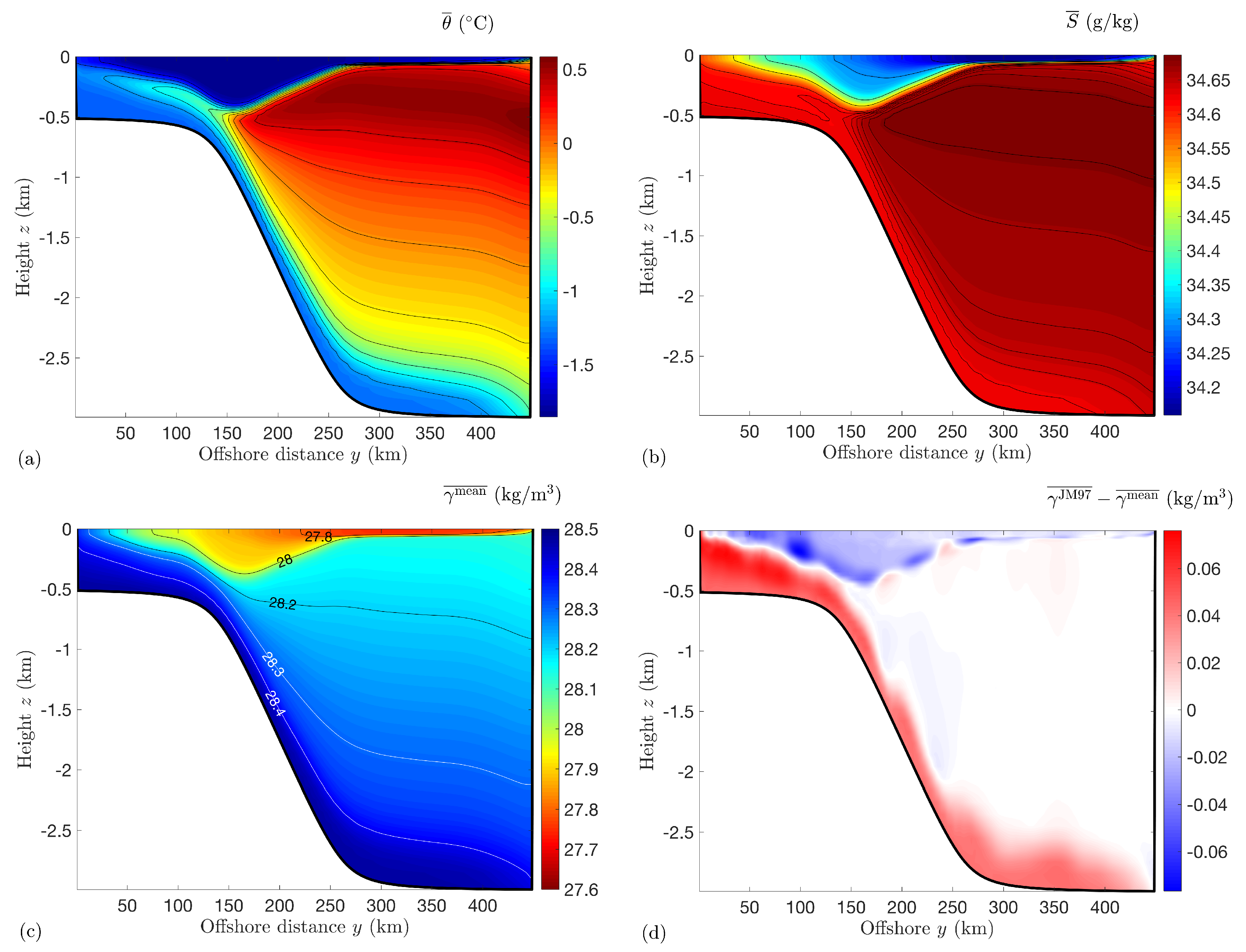
4.2. Constructing Neutral Density from the Model’s Mean State

To test the NTRM we must first construct ${\gamma }^{\mathrm{mean}}$, i.e., for each time $t_n$ and model grid location $(x_i,y_j,z_k)$ we must assign Neutral Densities ${\gamma }^{\mathrm{mean}}(x_i,y_j,z_k,t_n)$, where $i=1\dots N_x$, $j=1\dots N_y$, $k=1\dots N_z$, and $n=1\dots N_t$ are gridpoint indices. Similar to the procedure laid out by [24], we require a dataset to which the instantaneous model stratification can be referred in order to assign a ${\gamma }^{\mathrm{mean}}$ value to each grid point. In [24], this dataset was the hydrographic climatology of [45] and a corresponding set of neutral density labels on a coarse global grid. Similarly, for the purpose of constructing ${\gamma }^{\mathrm{mean}}$ the reference dataset is the model’s time-mean hydrography, $\overline{S}(y_j,z_k)$ and $\overline{\theta }(y_j,z_k)$ (see Figure 1a,b), and a corresponding set of neutral density labels ${\gamma }_{\mathrm{ref}}^{\mathrm{mean}}(y_j,z_k)$. Note that the reference dataset is approximately independent of x due to the zonally symmetric model geometry and forcing. The approximate two-dimensionality of the time-mean hydrography also implies that the neutral helicity of the reference dataset is zero [29]. Taken together with the simply connected model domain, this implies that Neutral Surfaces are well defined [46].

We now outline the procedure for labeling the reference dataset with ${\gamma }_{\mathrm{ref}}^{\mathrm{mean}}$ and assigning ${\gamma }^{\mathrm{mean}}$ values to instantaneous model output. This procedure closely follows that described by [24], to which the reader is referred for more specific details of the algorithm. We first labeled the northernmost model water column, ${\gamma }_{\mathrm{ref}}^{\mathrm{mean}}(y_{N_y},z_k)$, by setting it equal to ${\gamma }^{\mathrm{JM}97}(y_{N_y},z_k)$. Here ${\gamma }^{\mathrm{JM}97}$ was calculated from the hydrographic measurements used to restore the model stratification in the offshore sponge layer, taking the model domain to lie along a slice between (61W,67S) at $y=0$ and (50.6W,67S) at $y=450\mathrm{km}$ [23]. We then iterated southward through the model water columns, assigning the $j^{\mathrm{th}}$ column, $\left\{{\gamma }_{\mathrm{ref}}^{\mathrm{mean}}(y_j,z_k)|k=1\dots N_z\right\}$, from the ${(j+1)}^{\mathrm{th}}$ column using the form of the discrete neutral relation (7) given by [24] and linear vertical interpolation. For grid points in the $j^{\mathrm{th}}$ column that were denser or lighter than any grid point in the ${(j+1)}^{\mathrm{th}}$ water column, we linearly extrapolated ${\gamma }_{\mathrm{ref}}^{\mathrm{mean}}(y_j,z_k)$ vertically. Note that in our vertical density extrapolation we assigned the vertical gradient of ${\gamma }_{\mathrm{ref}}^{\mathrm{mean}}$ to be equal to the vertical gradient of locally-referenced potential density, whereas in this region the vertical gradient of ${\gamma }^{\mathrm{JM}97}$ was typically assigned to be twice the vertical gradient of locally-referenced potential density (the “b-factor” of [24]). This choice of extrapolation was made for simplicity and should not influence our results, though a consequence is that ${\gamma }^{\mathrm{mean}}$ spans a smaller range of density values than ${\gamma }^{\mathrm{JM}97}$ in this model domain.

To calculate ${\gamma }^{\mathrm{mean}}(x_i,y_j,z_k,t_n)$ for a given model gridpoint with salinity $S(x_i,y_j,z_k,t_n)$ and potential temperature $\theta (x_i,y_j,z_k,t_n)$, we construct continuous functions of z, $\overline{S}(y_j,z)$ and $\overline{\theta }(y_j,z)$, via linear interpolation. We then find a depth $z_r$ such that ($\overline{S}(y_j,z_r),\overline{\theta }(y_j,z_r),z_r)$ and $(S(x_i,y_j,z_k,t_n),\theta (x_i,y_j,z_k,t_n),z_k)$ satisfy the discrete neutral relation. We then assigned ${\gamma }^{\mathrm{mean}}(x_i,y_j,z_k,t_n)$ by linear vertical interpolation of ${\gamma }_{\mathrm{ref}}^{\mathrm{mean}}(y_j,z_k)$ to the point $z_{\mathrm{ref}}$. Note that our algorithm for assigning ${\gamma }^{\mathrm{mean}}$ differs slightly from the algorithm of [24] for assigning ${\gamma }^{\mathrm{JM}97}$: to assign ${\gamma }^{\mathrm{mean}}$ we refer each gridpoint to a horizontally local “cast” consisting of the Eulerian-mean model properties, whereas the algorithm of [24] refers each gridpoint to a four geographically local reference casts. Additionally, we use linear vertical interpolation to assign a ${\gamma }^{\mathrm{JM}97}$ value, whereas the algorithm of [24] uses quadratic interpolation.

In Figure 1a,b we plot the time- and zonal-mean potential temperature and salinity, $\overline{\theta }$ and $\overline{S}$, that serve as the reference dataset in the construction of ${\gamma }^{\mathrm{mean}}$. The mean state is qualitatively similar to hydrographic measurements from the western Weddell Sea [41], and exhibits a layer of relatively cold, fresh, shelf-sourced bottom water that descends down the continental slope. Figure 1c shows the time and zonal mean of the Neutral Density constructed from the model’s mean state, i.e., $\overline{{\gamma }^{\mathrm{mean}}}$, while Figure 1d shows the difference between $\overline{{\gamma }^{\mathrm{JM}97}}$ and $\overline{{\gamma }^{\mathrm{mean}}}$. As expected, ${\gamma }^{\mathrm{JM}97}$ takes lower values than ${\gamma }^{\mathrm{mean}}$ in waters lighter than the lightest water at the northern boundary, and higher values than ${\gamma }^{\mathrm{mean}}$ in waters denser than the densest water at the northern boundary, due to the procedure for extrapolating ${\gamma }_{\mathrm{ref}}^{\mathrm{mean}}$. Some variations are visible across the continental slope due to the presence of alternating along-slope jets that slowly drift offshore, and which do not perfectly cancel under integration over the 5-year analysis period [42].

We anticipate that ${\gamma }^{\mathrm{mean}}$ should be more closely aligned with local Neutral Surfaces than ${\gamma }^{\mathrm{JM}97}$. To illustrate this, in Figure 2 we plot the $\overline{{\gamma }^{\mathrm{mean}}}$, $\overline{{\gamma }^{\mathrm{JM}97}}$, $\overline{\theta }$ and $\overline{S}$ at the sea floor as a function of cross-slope distance, i.e., within the dense outflowing layer of shelf-sourced bottom water. Figure 2 shows that $\overline{{\gamma }^{\mathrm{JM}97}}$ exhibits spurious fluctuations and local minima, on the order of $0.01\mathrm{kg}{\mathrm{m}}^{-3}$, that are absent in $\overline{{\gamma }^{\mathrm{mean}}}$. For example, around $y=200\mathrm{km}$ there are negligible variations in $\overline{\theta }$ and $\overline{S}$, indicating that the sea floor should coincide with a neutral surface. This is reflected in $\overline{{\gamma }^{\mathrm{mean}}}$, but not in $\overline{{\gamma }^{\mathrm{JM}97}}$, which exhibits a spurious local minimum at this point. We conclude that iso-surfaces of ${\gamma }^{\mathrm{mean}}$ are more closely aligned with local Neutral Surfaces than ${\gamma }^{\mathrm{JM}97}$, though the spurious variations in ${\gamma }^{\mathrm{JM}97}$ are nonetheless quite small compared to the domain-scale ranges of ${\gamma }^{\mathrm{mean}}$ and ${\gamma }^{\mathrm{JM}97}$.

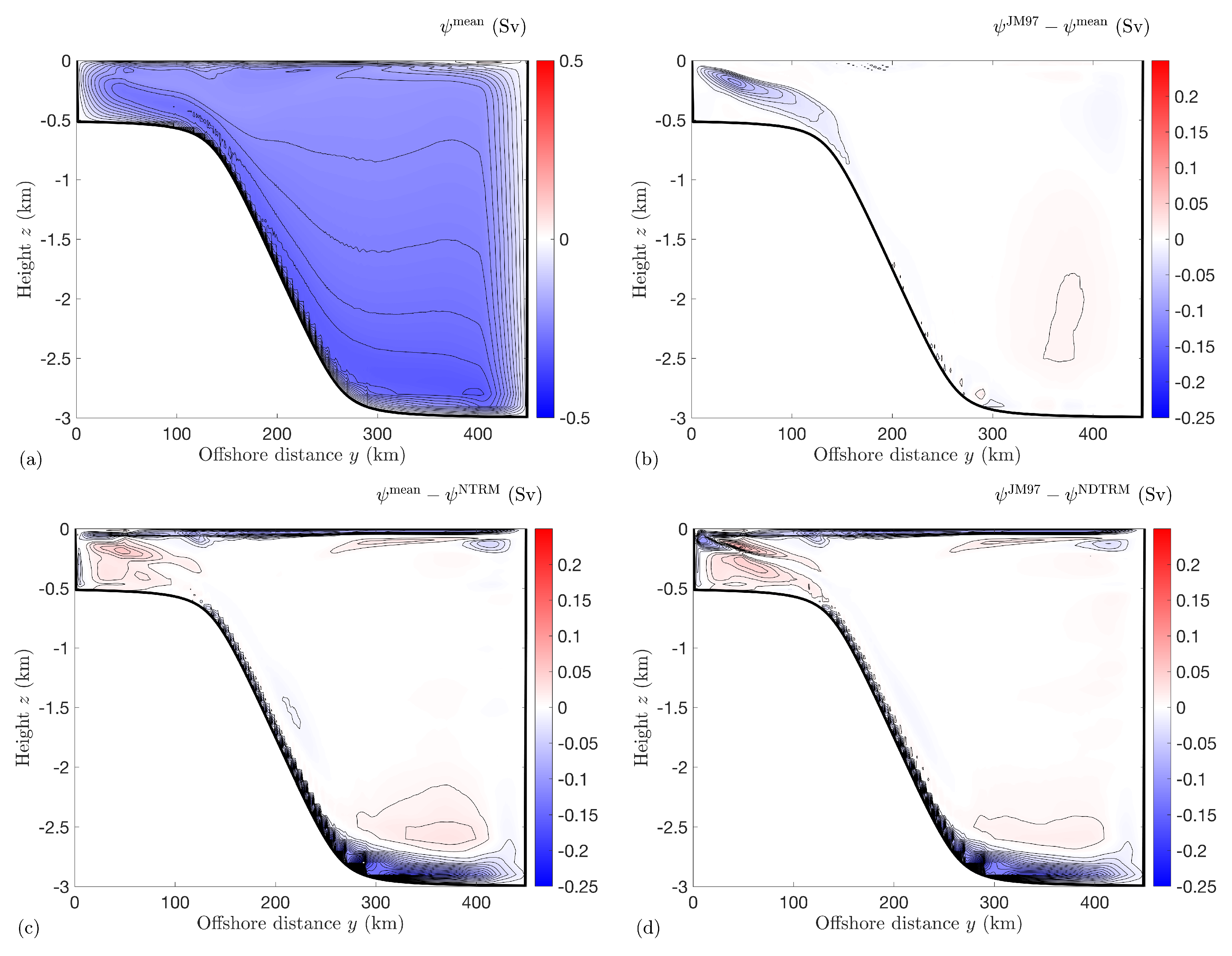
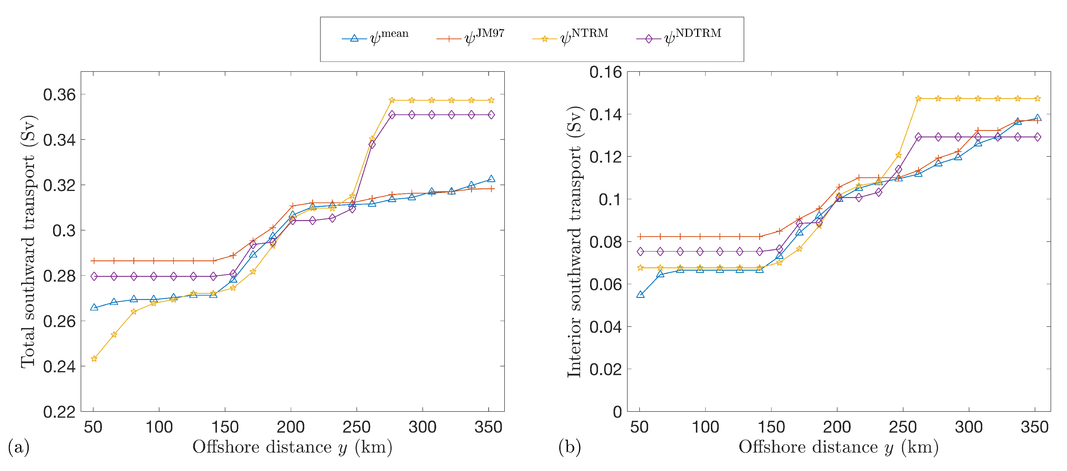
4.3. Comparing Diagnosed and TRM Transports

Having constructed ${\gamma }^{\mathrm{mean}}$, we now compare the transports within ${\gamma }^{\mathrm{mean}}$ and ${\gamma }^{\mathrm{JM}97}$ surfaces, as estimated by the TRM and diagnosed directly from the model simulations. Based on Section 3, we anticipate that the NTRM should more closely approximate the diagnosed fluxes within ${\gamma }^{\mathrm{mean}}$ surfaces, while the NDTRM should more closely approximate the diagnosed fluxes within ${\gamma }^{\mathrm{JM}97}$ surfaces.

We diagnose fluxes within density surfaces via direct calculation of (1). The procedure is summarized here to achieve a self-contained presentation; for further details the reader is referred to ST15. For each model snapshot, the model-reported meridional volume fluxes and Neutral Density (${\gamma }^{\mathrm{mean}}$ or ${\gamma }^{\mathrm{JM}97}$) on geopotential surfaces are interpolated to a vertical grid that is 10 times finer than the model’s vertical grid (see [23,41,42]). The volume fluxes are then assigned to a discrete set of density bins, averaged in time to compute mean volume fluxes within density surfaces, and integrated vertically in density space to obtain the streamfunction. To map the streamfunction back to z-space, we also average the height $z_0$ of each density surface, and map the streamfunction at density ${\gamma }_0$ to height $\overline{z_0}$. This allows for direct comparison with the TRM, which approximates the transport above the isopycnal whose mean elevation is $\overline{z_0}$. Note that due to the zonal symmetry of the model domain, we only calculate the meridional component of the streamfunction, which quantifies circulation in the y/z plane. We denote the streamfunction corresponding to volume fluxes in ${\gamma }^{\mathrm{mean}}$ surfaces as ${\psi }^{\mathrm{mean}}$, and the streamfunction corresponding to volume fluxes in ${\gamma }^{\mathrm{JM}97}$ surfaces as ${\psi }^{\mathrm{JM}97}$.

We compare ${\psi }^{\mathrm{mean}}$ and ${\psi }^{\mathrm{JM}97}$ with the NTRM and NDTRM estimates of the volume fluxes. The NTRM is evaluated as the meridional component of (24), with the mean operator defined as a time and zonal average. We denote the resulting streamfunction as ${\psi }^{\mathrm{NTRM}}$. The NDTRM streamfunction is defined following equation (B.4) of ST15, and is denoted as ${\psi }^{\mathrm{NDTRM}}$. Throughout this section we use “NDTRM” to refer to the NDTRM2 of ST15, which was shown to exhibit closer agreement with diagnosed fluxes in ${\gamma }^{\mathrm{JM}97}$ surfaces than lower-order formulations of the NDTRM.

In Figure 3 we compare ${\psi }^{\mathrm{mean}}$ and ${\psi }^{\mathrm{JM}97}$, ${\psi }^{\mathrm{NTRM}}$ and ${\psi }^{\mathrm{NDTRM}}$ directly. Figure 3a shows the overturning circulation diagnosed from volume fluxes within ${\gamma }^{\mathrm{mean}}$ surfaces. The circulation is characterized by wind-driven shoreward transport within the surface mixed layer and shoreward interior eddy transport across the continental slope [42]. These shoreward transports are returned offshore via dense shelf water export down the continental slope. Figure 3 quantifies the difference in the computed transports within ${\gamma }^{\mathrm{mean}}$ and ${\gamma }^{\mathrm{JM}97}$ surfaces. The most substantial difference is that the amplitude of ${\psi }^{\mathrm{JM}97}$ is enhanced relative to ${\psi }^{\mathrm{mean}}$ over the upper continental slope and the continental shelf, exceeding the ∼0.23$\mathrm{Sv}$ shelf overturning magnitude of ${\psi }^{\mathrm{mean}}$ by around $0.08\mathrm{Sv}$. This suggests that a non-negligible fraction of the diagnosed shelf overturning in ${\psi }^{\mathrm{JM}97}$ surfaces is due to errors introduced by the independent reference dataset of [24]. Figure 3c,d show the differences between ${\psi }^{\mathrm{mean}}$ and ${\psi }^{\mathrm{NTRM}}$, and between ${\psi }^{\mathrm{JM}97}$ and ${\psi }^{\mathrm{NDTRM}}$, respectively. Both TRM streamfunctions somewhat underestimate the amplitude of the overturning circulation over the continental shelf, and also exhibit errors close to the ocean surface and floor, where the vertical stratification is weak. The latter might be ameliorated by adopting a generalized form of the NTRM that utilizes vertical tracer fluxes in weakly-stratified regions, analogous to the methods proposed by [47,48]. The errors are typically smaller than $0.05\mathrm{Sv}$ in magnitude, which is smaller than the difference between ${\psi }^{\mathrm{mean}}$ and ${\psi }^{\mathrm{JM}97}$ over the shelf, suggesting that ${\psi }^{\mathrm{NTRM}}$ more closely approximates ${\psi }^{\mathrm{mean}}$ and that ${\psi }^{\mathrm{NDTRM}}$ more closely approximates ${\psi }^{\mathrm{JM}97}$.

To quantify the agreement between the TRM and diagnosed transports, in Figure 4a we compare the net southward transport reported by each streamfunction, as a function of latitude. This calculation follows ST15, and only includes southward transport at any given latitude if that transport has been supplied from the northern boundary of the domain, i.e., only counting streamlines that connect that latitude to the northern boundary. Figure 4b shows a similar comparison, but only accounting for southward interior transport, i.e., excluding transport in the surface mixed layer. In each case, ${\psi }^{\mathrm{NTRM}}$ and ${\psi }^{\mathrm{NDTRM}}$ more closely tracks ${\psi }^{\mathrm{mean}}$ and ${\psi }^{\mathrm{JM}97}$, respectively, over the continental slope ($y\lesssim 150\mathrm{km}$). Over the continental slope ($150\mathrm{km}\lesssim y\lesssim 250\mathrm{km}$) the transports are difficult to distinguish, as suggested by Figure 3. In the deep ocean ($y\gtrsim 250\mathrm{km}$) the TRM and diagnosed transports diverge due to large differences in the streamfunctions close to the sea floor (see Figure 3c,d). Thus, our net southward transport metrics confirm the result suggested by the overturning streamfunction comparison in Figure 3: the NTRM more closely approximates volume fluxes in ${\psi }^{\mathrm{mean}}$ surfaces, while the NDTRM more closely approximates fluxes in ${\psi }^{\mathrm{JM}97}$ surfaces.

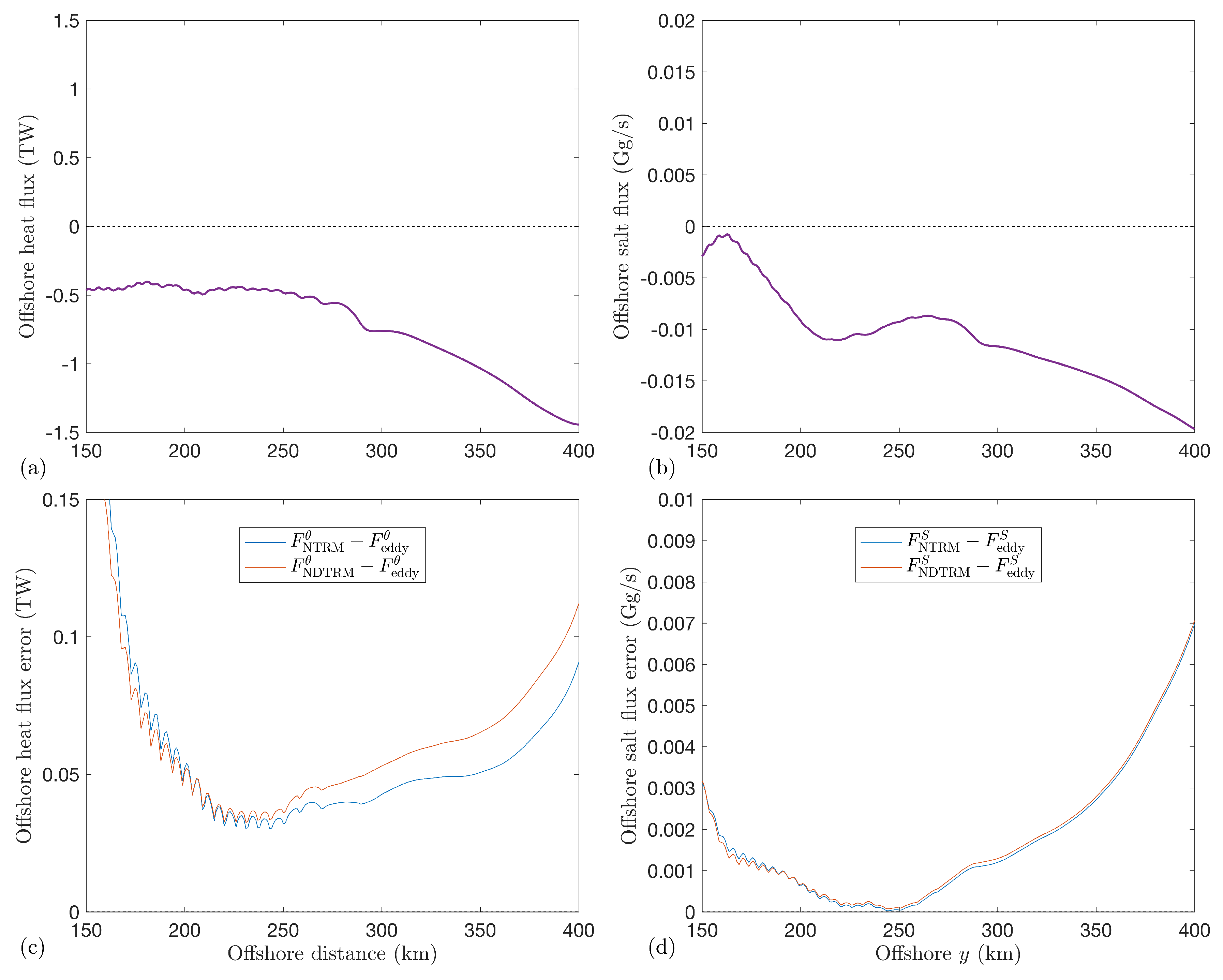
4.4. Advective Tracer Transport

Finally, we note that that in addition to estimating isopycnal/diapycnal transports, TRM streamfunctions may also be used to estimate the advective flux of tracers. Importantly, no globally-defined density variable is needed to perform such an estimate, so, e.g., it would not be necessary to construct a Neutral Density variable like ${\gamma }^{\mathrm{mean}}$ in conjunction with the NTRM for this purpose. We now compare the advective meridional fluxes of $\theta$ and S estimated by the NTRM and NDTRM with those diagnosed from the model simulation. We focus on the continental shelf and open ocean regions ($y\gtrsim 150\mathrm{km}$), in which the heat and salt transports have been shown to be primarily advective, rather than diffusive [42].

Figure 5a,b shows the northward eddy fluxes of heat and salt, diagnosed directly from the daily model output via

$$F_{\mathrm{eddy}}^{\chi }=L_x{\int }_{-h}^0\overline{v^{\prime }{\chi }^{\prime }}\mathrm{d}z.$$

(45)

Here $\chi =\theta$ or $\chi =S$, $z=-h\left(y\right)$ is the sea floor elevation, the mean operator $\overline{•}$ denotes a time and zonal average, and primes ′ denote deviations from that average. The heat and salt fluxes have been rescaled to take units of $\mathrm{TW}$ and $\mathrm{Gg}/\mathrm{s}$, respectively, for ease of interpretation. We calculate NTRM and NDTRM estimates of the advective fluxes via

$$F_{\mathrm{TRM}}^{\chi }=-L_x{\int }_{-h}^0\frac{\partial {\psi }_{\mathrm{TRM}}}{\partial z}\overline{\chi }\mathrm{d}z.$$

(46)

Here we set ${\psi }_{\mathrm{TRM}}={\psi }^{\mathrm{NTRM}}$ and ${\psi }_{\mathrm{TRM}}={\psi }^{\mathrm{NDTRM}}$ to define the flux estimates $F_{\mathrm{NTRM}}^{\chi }$ and $F_{\mathrm{NDTRM}}^{\chi }$, respectively. In Figure 5c,d we plot the differences between the diagnosed and TRM-estimated heat and salt fluxes, which typically differ by around 10–20%. There is very little difference between the NTRM and NDTRM salt fluxes, whereas the NTRM yields errors in the heat flux that are up to 40% smaller than the errors incurred by using the NDTRM.

5. Summary and Conclusions

The Temporal Residual Mean (TRM) transport requires an Eulerian approximation for vertical fluctuations of a set of quasi-material surfaces (e.g., [20,21,22]). The TRM approximates the transport within these surfaces, which in turn approximates the semi-Lagrangian mean and Lagrangian-mean transports [9]. This article builds on a recent study by [23] (hereafter ST15), who used the Neutral Density variable ${\gamma }^{\mathrm{JM}97}$ of [24] to construct a Neutral Density TRM (NDTRM) that can be applied anywhere in the ocean, circumventing the limitations of e.g., potential density at high latitudes. A key result of this article is that the vertical fluctuations of local Neutral Surfaces, which are defined directly via the continuous form of the neutral relation, can be approximated via (23). The corresponding TRM streamfunction (24), referred to as the “Neutral TRM” (NTRM) should more closely approximate the semi-Lagrangian mean transport than the NDTRM, and therefore also better approximate the generalized Lagrangian mean transport [9]. The NTRM also coincides with a TRM based on vertical fluctuations of locally-referenced potential density surfaces, again to the same asymptotic order in the amplitude of the isopycnal height fluctuations.

In isolation the NTRM streamfunction does not directly quantify isopycnal and diapycnal ocean transports (see e.g., [31]) because local Neutral Surfaces are, by definition, not globally well-defined. However, in Section 3 we showed for the special case of a Neutral Density variable (${\gamma }^{\mathrm{mean}}$) constructed using the Eulerian-mean ocean state, the NDTRM reduces to the NTRM, up to the same asymptotic order in the amplitude of the isopycnal height fluctuations. Thus the NTRM approximately quantifies adiabatic and diabatic volume fluxes within and across ${\gamma }^{\mathrm{mean}}$ surfaces, again up to a consistent asymptotic order in the amplitude of the isopycnal height fluctuations.

In Section 4 we tested this theoretical prediction explicitly using an idealized eddy-resolving simulation of the Antarctic continental shelf and slope. Using the model’s time-mean state as a reference dataset for ${\gamma }^{\mathrm{mean}}$, we labeled the model output with both ${\gamma }^{\mathrm{mean}}$ and ${\gamma }^{\mathrm{JM}97}$ and computed volume fluxes within surfaces of both Neutral Density variables. We showed that ${\gamma }^{\mathrm{mean}}$ iso-surfaces were more closely aligned with local Neutral Surfaces than ${\gamma }^{\mathrm{JM}97}$, indicating that fluxes within ${\gamma }^{\mathrm{mean}}$ surfaces should be more closely aligned with the local neutral tangent plane. Consistent with Section 3, we found that the NTRM more closely approximated volume fluxes within ${\gamma }^{\mathrm{mean}}$ surfaces, while the NDTRM more closely approximated volume fluxes within ${\gamma }^{\mathrm{JM}97}$ surfaces. Finally, we compared the advective fluxes of heat and salt estimated by the NTRM and NDTRM, with those diagnosed from the model. Both formulations of the TRM yielded flux estimates in close agreement with the diagnosed fluxes, though the NTRM yielded a somewhat closer approximation to the heat fluxes.

The results summarized above suggest that for most oceanographic purposes, the NTRM is preferable to the NDTRM for the purposes of estimating isopycnal and diapycnal volume fluxes, and of estimating advective tracer fluxes. It also bears the advantage of being more convenient to compute than the NDTRM, as it makes no explicit reference to globally-defined Neutral Density variable or to the set of reference casts used to defined such a variable. A practical consideration is that the NTRM advects a Neutral Density variable constructed from the model’s time-mean state, i.e., ${\gamma }^{\mathrm{mean}}$ [22]. Though algorithms for constructing global, approximately neutral density variables have been proposed (e.g., [24,49,50]), translating these algorithms to the time-mean state of a three-dimensional model with an arbitrary ocean geometry is non-trivial. More recent algorithms have been proposed to construct global, approximately neutral surfaces [46,51], but have not yet been adapted to the construction of three-dimensional Neutral Density variables. Furthermore, a Neutral Density variable such as ${\gamma }^{\mathrm{mean}}$ would need to be constructed with great care to achieve consistency with ${\gamma }^{\mathrm{JM}97}$, which has been used to map the global overturning circulation [5,25].

Throughout this manuscript we have assumed that local Neutral Surfaces coincide with purely adiabatic flows [26], and are therefore optimal for the construction of the TRM. Neutral helicity precludes the construction of a continuous density variable that lies exactly parallel to these surfaces everywhere in the ocean [29]. However, on the basis of two-parcel energetic considerations, Ref. [52] argued that that adiabatic parcel displacements should not, in fact, follow the neutral tangent plane. Variance of potential temperature and salinity has been found to be larger on Neutral Density surfaces than on surfaces of potential density referenced to 2000 decibars [26,53], though this does not explicitly contradict the notion that adiabatic parcel displacements follow neutral surfaces. Although this topic remains under debate [54,55,56], an implication is that there may yet be a more accurate choice than local Neutral Surfaces to define adiabatic heaving, and therefore to approximate the semi-Lagrangian mean and generalized Lagrangian mean transports. Further work is required to compare estimates of thickness-weighted average transports within different formulations of quasi-neutral surfaces, such as $\omega$-surfaces [51], thermodynamic neutral density (${\gamma }^T$) surfaces [50], and orthobaric density surfaces [49].

Previous studies have used the NTRM0, and thus implicitly the NTRM (see Section 3), to estimate volume fluxes within ${\gamma }^{\mathrm{JM}97}$ surfaces (e.g., [42,57,58,59]). In principle, this incurs an $\mathcal{O}\left(\tilde{\Delta }\right)$ error in the approximation, where $\tilde{\Delta }$ quantifies differences between the model’s mean state and the independent reference dataset. On the other hand, our comparison in Section 4 shows that the NTRM approximates transports within ${\gamma }^{\mathrm{JM}97}$ surfaces almost as closely as it approximates transports within ${\gamma }^{\mathrm{mean}}$ surfaces, so in practice such errors may not be of concern. However, further work is required to evaluate errors associated with neutral helicity when quantifying transports within ${\gamma }^{\mathrm{mean}}$ surfaces using the NTRM.

References

1. Srokosz, M.; Baringer, M.; Bryden, H.; Cunningham, S.; Delworth, T.; Lozier, S.; Marotzke, J.; Sutton, R. Past, present, and future changes in the Atlantic meridional overturning circulation. Bull. Am. Meteorol. Soc. 2012, 93, 1663–1676. [Google Scholar] [CrossRef]
2. Marshall, J.; Speer, K. Closure of the meridional overturning circulation through Southern Ocean upwelling. Nat. Geosci. 2012, 5, 171–180. [Google Scholar] [CrossRef] [Green Version]
3. Döös, K.; Webb, D.J. The Deacon cell and the other meridional cells of the Southern Ocean. J. Phys. Oceanogr. 1994, 24, 429–442. [Google Scholar] [CrossRef]
4. Hirst, A.C.; McDougall, T.J. Deep-water properties and surface buoyancy flux as simulated by a z-coordinate model including eddy-induced advection. J. Phys. Oceanogr. 1996, 26, 1320–1343. [Google Scholar] [CrossRef]
5. Lumpkin, R.; Speer, K. Global ocean meridional overturning. J. Phys. Oceanogr. 2007, 37, 2550–2562. [Google Scholar] [CrossRef]
6. Wolfe, C.L.; Cessi, P. Overturning circulation in an eddy-resolving model: The effect of the pole-to-pole temperature gradient. J. Phys. Oceanogr. 2009, 39, 125–142. [Google Scholar] [CrossRef]
7. Sun, S.; Eisenman, I.; Stewart, A.L. The influence of Southern Ocean surface buoyancy forcing on glacial-interglacial changes in the global deep ocean stratification. Geophys. Res. Lett. 2016, 43, 8124–8132. [Google Scholar] [CrossRef]
8. Sun, S.; Eisenman, I.; Stewart, A.L. Does Southern Ocean surface forcing shape the global ocean overturning circulation? Geophys. Res. Lett. 2018, 45, 2413–2423. [Google Scholar] [CrossRef]
9. Eden, C. Relating Lagrangian, residual, and isopycnal means. J. Phys. Oceanogr. 2012, 42, 1057–1064. [Google Scholar] [CrossRef]
10. Plumb, R.A. Eddy fluxes of conserved quantities by small-amplitude waves. J. Atmos. Sci. 1979, 36, 1699–1704. [Google Scholar] [CrossRef]
11. Marshall, J.; Radko, T. Residual-mean solutions for the Antarctic Circumpolar Current and its associated overturning circulation. J. Phys. Oceanogr. 2003, 33, 2341–2354. [Google Scholar] [CrossRef]
12. Abernathey, R.; Marshall, J.; Ferreira, D. The dependence of Southern Ocean meridional overturning on wind stress. J. Phys. Oceanogr. 2011, 41, 2261–2278. [Google Scholar] [CrossRef]
13. Stewart, A.L.; Hogg, A.M. Reshaping the Antarctic Circumpolar Current via Antarctic Bottom Water Export. J. Phys. Oceanogr. 2017, 47, 2577–2601. [Google Scholar] [CrossRef]
14. Nikurashin, M.; Vallis, G. A theory of deep stratification and overturning circulation in the ocean. J. Phys. Oceanogr. 2011, 41, 485–502. [Google Scholar] [CrossRef]
15. Nikurashin, M.; Vallis, G. A theory of the interhemispheric meridional overturning circulation and associated stratification. J. Phys. Oceanogr. 2012, 42, 1652–1667. [Google Scholar] [CrossRef]
16. Stewart, A.L.; Ferrari, R.; Thompson, A.F. On the importance of surface forcing in conceptual models of the deep ocean. J. Phys. Oceanogr. 2014, 44, 891–899. [Google Scholar] [CrossRef]
17. Burke, A.; Stewart, A.L.; Adkins, J.F.; Ferrari, R.; Jansen, M.F.; Thompson, A.F. The glacial mid-depth radiocarbon bulge and its implications for the overturning circulation. Paleoceanography 2015, 30, 1021–1039. [Google Scholar] [CrossRef] [Green Version]
18. Watson, A.J.; Vallis, G.K.; Nikurashin, M. Southern Ocean buoyancy forcing of ocean ventilation and glacial atmospheric CO2. Nat. Geosci. 2015, 8, 861–864. [Google Scholar] [CrossRef]
19. Thompson, A.F.; Stewart, A.L.; Bischoff, T. A multibasin residual-mean model for the global overturning circulation. J. Phys. Oceanogr. 2016, 46, 2583–2604. [Google Scholar] [CrossRef]
20. McDougall, T.J.; McIntosh, P.C. The temporal-residual-mean velocity. Part I: Derivation and the scalar conservation equations. J. Phys. Oceanogr. 1996, 26, 2653–2665. [Google Scholar] [CrossRef]
21. McDougall, T.J.; McIntosh, P.C. The temporal-residual-mean velocity. Part II: Isopycnal interpretation and the tracer and momentum equations. J. Phys. Oceanogr. 2001, 31, 1222–1246. [Google Scholar] [CrossRef]
22. Wolfe, C.L. Approximations to the ocean’s residual circulation in arbitrary tracer coordinates. Ocean Model. 2014, 75, 20–35. [Google Scholar] [CrossRef]
23. Stewart, A.L.; Thompson, A.F. The Neutral Density Temporal Residual Mean overturning circulation. Ocean Model. 2015, 90, 44–56. [Google Scholar] [CrossRef] [Green Version]
24. Jackett, D.R.; McDougall, T.J. A neutral density variable for the world’s oceans. J. Phys. Oceanogr. 1997, 27, 237–263. [Google Scholar] [CrossRef]
25. Talley, L.D. Closure of the global overturning circulation through the Indian, Pacific, and Southern Oceans: Schematics and transports. Oceanography 2013, 26, 80–97. [Google Scholar] [CrossRef]
26. McDougall, T.J. Neutral surfaces. J. Phys. Oceanogr. 1987, 17, 1950–1964. [Google Scholar] [CrossRef]
27. Iselin, C.O. The influence of vertical and lateral turbulence on the characteristics of the waters at mid-depths. Eos Trans. Am. Geophys. Union 1939, 20, 414–417. [Google Scholar] [CrossRef]
28. McDougall, T.J.; Groeskamp, S.; Griffies, S.M. On geometrical aspects of interior ocean mixing. J. Phys. Oceanogr. 2014, 44, 2164–2175. [Google Scholar] [CrossRef]
29. McDougall, T.J.; Jackett, D.R. On the helical nature of neutral trajectories in the ocean. Prog. Oceanogr. 1988, 20, 153–183. [Google Scholar] [CrossRef]
30. Eden, C.; Willebrand, J. Neutral density revisited. Deep Sea Res. Part II Top. Stud. Oceanogr. 1999, 46, 33–54. [Google Scholar] [CrossRef]
31. Groeskamp, S.; Griffies, S.M.; Iudicone, D.; Marsh, R.; Nurser, A.J.G.; Zika, J.D. The water mass transformation framework for ocean physics and biogeochemistry. Ann. Rev. Mar. Sci. 2019, 11, 271–305. [Google Scholar] [CrossRef] [PubMed]
32. Andrews, D.G.; McIntyre, M.E. An exact theory of nonlinear waves on a Lagrangian-mean flow. J. Fluid Mech. 1978, 89, 609–646. [Google Scholar] [CrossRef] [Green Version]
33. Young, W.R. An exact thickness-weighted average formulation of the Boussinesq equations. J. Phys. Oceanogr. 2012, 42, 692–707. [Google Scholar] [CrossRef]
34. Groeskamp, S.; Barker, P.M.; McDougall, T.J.; Abernathey, R.P.; Griffies, S.M. VENM: An Algorithm to Accurately Calculate Neutral Slopes and Gradients. J. Adv. Model. Earth Syst. 2019, 11, 1917–1939. [Google Scholar] [CrossRef] [Green Version]
35. Groeskamp, S.; Iudicone, D. The Effect of Air-Sea Flux Products, Shortwave Radiation Depth Penetration, and Albedo on the Upper Ocean Overturning Circulation. Geophys. Res. Lett. 2018, 45, 9087–9097. [Google Scholar] [CrossRef]
36. McIntosh, P.C.; McDougall, T.J. Isopycnal averaging and the residual mean circulation. J. Phys. Oceanogr. 1996, 26, 1655–1660. [Google Scholar] [CrossRef]
37. Gill, A.E. Circulation and bottom water production in the Weddell Sea. Deep Sea Res. Oceanogr. 1973, 20, 111–140. [Google Scholar] [CrossRef]
38. Thompson, A.F.; Stewart, A.L.; Spence, P.; Heywood, K.J. The Antarctic slope current in a changing climate. Rev. Geophys. 2018, 56, 741–770. [Google Scholar] [CrossRef]
39. Stewart, A.L.; Thompson, A.F. Sensitivity of the ocean’s deep overturning circulation to easterly Antarctic winds. Geophys. Res. Lett. 2012, 39. [Google Scholar] [CrossRef]
40. Stewart, A.L.; Thompson, A.F. Connecting Antarctic cross-slope exchange with Southern Ocean overturning. J. Phys. Oceanogr. 2013, 43, 1453–1471. [Google Scholar] [CrossRef]
41. Stewart, A.L.; Thompson, A.F. Eddy-mediated transport of warm Circumpolar Deep Water across the Antarctic shelf break. Geophys. Res. Lett. 2015, 42, 432–440. [Google Scholar] [CrossRef]
42. Stewart, A.L.; Thompson, A.F. Eddy generation and jet formation via dense water outflows across the Antarctic continental slope. J. Phys. Oceanogr. 2016, 46, 3729–3750. [Google Scholar] [CrossRef]
43. Marshall, J.; Hill, C.; Perelman, L.; Adcroft, A. Hydrostatic, quasi-hydrostatic, and nonhydrostatic ocean modeling. J. Geophys. Res. Oceans 1997, 102, 5733–5752. [Google Scholar] [CrossRef]
44. Marshall, J.; Adcroft, A.; Hill, C.; Perelman, L.; Heisey, C. A finite-volume, incompressible Navier Stokes model for studies of the ocean on parallel computers. J. Geophys. Res. Oceans 1997, 102, 5753–5766. [Google Scholar] [CrossRef] [Green Version]
45. Levitus, S. Climatological atlas of the world ocean. Eos Trans. Am. Geophys. Union 1983, 64, 962–963. [Google Scholar] [CrossRef]
46. Stanley, G.J. Neutral surface topology. Ocean Model. 2019, 138, 88–106. [Google Scholar] [CrossRef] [Green Version]
47. Held, I.M.; Schneider, T. The surface branch of the zonally averaged mass transport circulation in the troposphere. J. Atmos. Sci. 1999, 56, 1688–1697. [Google Scholar] [CrossRef]
48. Colas, F.; Capet, X.; McWilliams, J.C.; Li, Z. Mesoscale eddy buoyancy flux and eddy-induced circulation in Eastern Boundary Currents. J. Phys. Oceanogr. 2013, 43, 1073–1095. [Google Scholar] [CrossRef]
49. De Szoeke, R.A.; Springer, S.R.; Oxilia, D.M. Orthobaric density: A thermodynamic variable for ocean circulation studies. J. Phys. Oceanogr. 2000, 30, 2830–2852. [Google Scholar] [CrossRef]
50. Tailleux, R. Generalized patched potential density and thermodynamic neutral density: Two new physically based quasi-neutral density variables for ocean water masses analyses and circulation studies. J. Phys. Oceanogr. 2016, 46, 3571–3584. [Google Scholar] [CrossRef]
51. Klocker, A.; McDougall, T.; Jackett, D. A new method for forming approximately neutral surfaces. Ocean Sci. 2009, 5, 155–172. [Google Scholar] [CrossRef] [Green Version]
52. Tailleux, R. Neutrality versus materiality: A thermodynamic theory of neutral surfaces. Fluids 2016, 1, 32. [Google Scholar] [CrossRef]
53. Van Sebille, E.; Baringer, M.O.; Johns, W.E.; Meinen, C.S.; Beal, L.M.; De Jong, M.F.; Van Aken, H.M. Propagation pathways of classical Labrador Sea water from its source region to 26 °N. J. Geophys. Res. Oceans 2011, 116. [Google Scholar] [CrossRef]
54. Tailleux, R. On the validity of single-parcel energetics to assess the importance of internal energy and compressibility effects in stratified fluids. J. Fluid Mech. 2015, 767. [Google Scholar] [CrossRef] [Green Version]
55. McDougall, T.; Groeskamp, S.; Griffies, S. Comment on Tailleux, R. Neutrality versus Materiality: A Thermodynamic Theory of Neutral Surfaces. Fluids 2016, 1, 32. [Google Scholar] [CrossRef]
56. Tailleux, R. Reply to “Comment on Tailleux, R. Neutrality Versus Materiality: A Thermodynamic Theory of Neutral Surfaces. Fluids 2016, 1, 32.”. Fluids 2017, 2, 20. [Google Scholar] [CrossRef]
57. Stewart, A.L.; Klocker, A.; Menemenlis, D. Circum-Antarctic Shoreward Heat Transport Derived From an Eddy-and Tide-Resolving Simulation. Geophys. Res. Lett. 2018, 45, 834–845. [Google Scholar] [CrossRef]
58. Palóczy, A.; Gille, S.T.; McClean, J.L. Oceanic heat delivery to the Antarctic continental shelf: Large-scale, low-frequency variability. J. Geophys. Res. Oceans 2018, 123, 7678–7701. [Google Scholar] [CrossRef]
59. Stewart, A.L.; Klocker, A.; Menemenlis, D. Acceleration and overturning of the Antarctic Slope Current by winds, eddies, and tides. J. Phys. Oceanogr. 2019, 49, 2043–2074. [Google Scholar] [CrossRef]
Figure 1. Diagnostics of the mean model state, where averages are taken in time (over 5 years of daily snapshots) and in the along-slope (zonal) direction ( 400 km distance at ∼1 km horizontal grid spacing. (a) Potential temperature θ , (b) practical salinity S, (c) Neutral Density constructed based on the model’s mean state, which we denote as γ mean (see Section 4), (d) difference between γ JM 97 ¯ , where γ JM 97 is the Neutral Density calculated using the reference dataset and algorithm of [24], and γ mean ¯ .
Fluids 04 00179 g001
Figure 2. Time-/alongshore-mean (a) γ mean , (b) γ JM 97 , (c) salinity and (d) potential temperature in the bottom-most model grid point, i.e., in the layer of dense water that descends down the continental slope [42], as a function of distance from the shore. This plot illustrates that the use of an independent reference dataset leads to a spurious local minima, e.g., around y = 200 km , in γ JM 97 . These are absent in γ mean , indicating that it more closely tracks Neutral Surfaces. The rapid density variations around y = 100 km are due to “steps” in the model’s geopotential-coordinate representation of the continental slope.
Fluids 04 00179 g002
Figure 3. Comparison of transports calculated via TRM approximations vs. diagnosed directly from model output by averaging within density surfaces. Transports are quantified via streamfunctions with blue colors corresponding to counter-clockwise circulation and black contours shown at intervals of (a) 0.025 Sv and (bd) 0.01 Sv . (a) Diagnosed transport within γ mean surfaces ( ψ mean ), (b) difference between diagnosed transports within γ JM 97 surfaces and γ mean surfaces ( ψ mean ψ JM 97 ), (c) difference between NTRM-estimated transport within γ mean surfaces and diagnosed transport within γ mean surfaces ( ψ NTRM ψ mean ), (d) difference between NDTRM-estimated transport within γ n surfaces and diagnosed transports within γ JM 97 surfaces ( ψ JM 97 ψ NDTRM ). The diagnosed streamfunctions, ψ mean and ψ JM 97 , have been mapped from density to z coordinates using the time-mean depths of γ mean and γ JM 97 surfaces, respectively.
Fluids 04 00179 g003
Figure 4. Comparison of total thickness-weighted average cross-slope transports calculated via TRM approximations vs. diagnosed directly from model output. (a) Total southward transport, (b) total interior southward transport, i.e., excluding wind-driven Ekman transport of surface waters (see Section 4 and [23]).
Fluids 04 00179 g004
Figure 5. Comparison between cross-slope heat and salt fluxes diagnosed directly from the model output vs. estimated using TRM streamfunctions (see Section 4). Fluxes are plotted over a subset of the model domain in which the eddy transport was found to be primarily advective, rather than diffusive [42]. (a,b) Diagnosed offshore heat and salt fluxes, respectively. (c,d) Differences between diagnosed and NTRM-/NDTRM-estimated offshore heat and salt fluxes, respectively.
Fluids 04 00179 g005