Turbulence Modeling Effects on the CFD Predictions of Flow over a Detailed Full-Scale Sedan Vehicle

Abstract

In today’s road vehicle design processes, Computational Fluid Dynamics (CFD) has emerged as one of the major investigative tools for aerodynamics analyses. The age-old CFD methodology based on the Reynolds Averaged Navier–Stokes (RANS) approach is still considered as the most popular turbulence modeling approach in automotive industries due to its acceptable accuracy and affordable computational cost for predicting flows involving complex geometries. This popular use of RANS still persists in spite of the well-known fact that, for automotive flows, RANS turbulence models often fail to characterize the associated flow-field properly. It is even true that more often, the RANS approach fails to predict correct integral aerodynamic quantities like lift, drag, or moment coefficients, and as such, they are used to assess the relative magnitude and direction of a trend. Moreover, even for such purposes, notable disagreements generally exist between results predicted by different RANS models. Thanks to fast advances in computer technology, increasing popularity has been seen in the use of the hybrid Detached Eddy Simulation (DES), which blends the RANS approach with Large Eddy Simulation (LES). The DES methodology demonstrated a high potential of being more accurate and informative than the RANS approaches. Whilst evaluations of RANS and DES models on various applications are abundant in the literature, such evaluations on full-car models are relatively fewer. In this study, four RANS models that are widely used in engineering applications, i.e., the realizable $k-\epsilon$ two-layer, Abe–Kondoh–Nagano (AKN) $k-\epsilon$ low-Reynolds, SST $k-\omega$, and V2F are evaluated on a full-scale passenger vehicle with two different front-end configurations. In addition, both cases are run with two DES models to assess the differences between the flow predictions obtained using RANS and DES.

1. Introduction

Since the last twenty years, Computational Fluid Dynamics (CFD) has played an important role in the early design stages of modern-day vehicles. In practice, Reynolds-Averaged Navier–Stokes (RANS) modeling still remains a widely-used approach in automotive applications of CFD, due to its acceptable accuracy, affordable cost, and fast turnaround time. However, due to the well-known drawbacks of RANS models in predicting complex separated flows, variants of the hybrid Detached Eddy Simulation (DES) approach are seen to gain popularity currently in many automotive applications. As demonstrated by many researchers [1,2,3], DES models generally offer an advantage over RANS models in better predicting the flow field and integral aerodynamic quantities like drag, lift, and moment coefficients. However, in spite of showing a superior flow prediction capability than the RANS approach, DES still cannot fully correctly capture the flow details. Additionally, the DES approach is still cost prohibitive for many applications; for example, for the recently developed DrivAer vehicle, the DES simulation is 17-times more expensive than the RANS computations [2]. In present day high-fidelity CFD analyses, simulations with 120 million cells are very common; even a RANS-based well-converged simulation of this size takes more 3000 core-hours for completion (see [4]), implying that a DES would have taken more than 50,000 core-hours for a single case. This makes the use DES analysis impractical for motorsports applications for sure and may be for the passenger vehicle industries as well. Subsequently, RANS approaches still remain a popular method in situations like the early design cycle of a new vehicle model where hundreds of design options need to be assessed.

In RANS approaches, the entire turbulence spectrum is approximated through a set of transport equations to solve the time-averaged mean flow field. These equations were established during the past several decades based on empiricism, mathematical analysis, and physical reasoning of the key mechanisms observed in canonical flows. RANS models have enjoyed remarkable success in various industrial applications. However, the inability of RANS models to predict complex separated flows correctly has motivated researchers to develop and apply higher order models in industrial applications. One promising model is the DES approach. DES is a hybrid modeling approach that combines the best of both RANS and LES: an RANS simulation in the viscosity-dominated boundary layers and an LES in the unsteady separated regions.

However, one major problem of the DES approach is how to deal with the spurious buffer layer between the RANS and Large Eddy Simulation (LES) regions [5,6]. Spalart et al. [7] proposed the Delayed Detached Eddy Simulation (DDES) to prevent DES from a too early switch to LES mode. Another modification is called the Improved Delayed Detached Eddy Simulation (IDDES), proposed by Shur et al. [8]. IDDES allows RANS to be used in a much thinner near-wall region and could provide the so-called Wall-Modeled LES (WMLES) capabilities to the DES formulation.

The existing literature contains a vast body of works on the evaluation of RANS and DES models for various flow configurations. Due to the scope of this study, only a few notable validation studies related to automotive flows will be discussed in this paper.

Due to the complexity and proprietary nature of the works associated with production passenger vehicles, the evaluations of turbulence models on full-scale vehicles are rare. Instead, researchers have mainly focused on simplified, generic car geometries, such as the Ahmed body [9] and the more recently introduced DrivAer models [10]. The Ahmed body was introduced in 1984 to analyze the key flow field features of ground vehicles [9]. The Ahmed body features a flat front with rounded corners and a sharp slanted rear upper surface with various angles. Since ground vehicles can be viewed as bluff bodies moving in close vicinity to the road, broad aerodynamic features of the Ahmed body resemble a ground vehicle, e.g., the flow separation on the rear window or the wake structure behind the body. The Ahmed body has been extensively studied by using both experimental and numerical methods. Until recently, it has been the most widely-used object for evaluation works on turbulence models related to automotive flows.

The main model variable for the Ahmed body geometry is the rear slant angle. The flow patterns on the rear slant and behind the body vary as the slant angle changes. Existing literature contains a vast amount of works that investigated the influence of the slant angle on the flow patterns. It was first shown by Ahmed et al. [9] in their introductory work on the Ahmed body that 30 degrees is the critical slant angle at which the topology of the flow is suddenly altered and the drag is reduced noticeably. Above this angle, the flow fully separates over the slant starting from its sharp edge due to the strong adverse pressure gradient between the slant and the roof. For such configurations, RANS models succeed in predicting the correct separation region, which agreed well with experimental data [2]. Below this critical angle, especially at 25 degrees, the flow is most complex. The flow still separates from the slant; however, the pressure gradient between the slant area and the side walls is still strong enough, which generates streamwise counter-rotating vortices at the lateral slant edges. These vortices induce a downward motion over the slant, mainly in the downstream part of the slant. Consequently, the flow that was partially detached from the upstream part of the slant can reattach further downstream, forming a confined recirculation zone over the rear slant. Moreover, the wake structures, which are dominated by the interactions between the separation zone and strong counter-rotating vortices, become very complex in this configuration. These vortices are also responsible for the high induced drag. Subsequently, the 25 degree slant angle model has become the most extensively studied variant of the Ahmed body geometry as it poses a significant challenge for CFD analyses. As demonstrated by [11,12,13,14], the majority of RANS models fail to predict the flow field past this 25 degree model correctly. These simulations either predict no separation or they cannot predict the correct size of the separation zone. Not only for RANS, the CFD simulation of the 25 degree Ahmed model is also challenging for the higher fidelity models, such as LES and hybrid LES/RANS [15]. For very small slant angles, i.e., smaller than 12 degrees, the flow is fully attached on the rear slant and only separates over the rear end of the body. For such simple flow patterns, most RANS models again perform very well in terms of both integrated quantities and flow structures [16]. To sum up, for the Ahmed car body, the performance of various turbulence models, especially RANS models, is highly influenced by the geometry and flow topology present. This raises the potential uncertainty in predicting automotive flows when using numerical approaches, especially RANS approaches.

A new realistic generic car model, called the DrivAer model, was proposed recently by the Institute of Aerodynamics and Fluid Mechanics of the Technical University of Munich (TUM), in cooperation with BMW and Audi AG. The DrivAer model is available in three typical car configurations, i.e., estate, fastback, and notchback. All three of these configurations have been experimentally investigated to provide data for numerical comparisons [10,17]. TUM researchers also investigated the fastback configuration numerically using the SST $k-\omega$ turbulence model [18]. These studies found that although there are good agreements for drag coefficients between the experiment and simulation, observable discrepancies in pressure distributions on the top and bottom of the car exist between the CFD simulation and experiment results. A recent work by Peters et al. [19], which presented higher order structured finite difference solutions using overset grids and NASA’s overset grid solver Overflow, also observed similar pressure distribution differences when using the SST $k-\omega$ model. Moreover, several widely-used RANS and hybrid LES/RANS models were also applied to the DrivAer model [1,2,20,21]. It was found that RANS models were unable to predict the force coefficients correctly, especially the lift coefficient. In addition, these studies indicated that, while inaccuracies still exist when compared to the experimental data, hybrid approaches predict both force coefficients and flow fields with better experimental correlations, but at the expense of much higher computational cost.

However, the evaluations of turbulence models on full-car geometries are quite rare. A recent work presented a study of RANS turbulence models on the prediction of aerodynamic characteristics of a NASCAR Gen-6 Cup race car [22]; this work showed that discernible differences in the predicted flow features, especially in the wake region, exist between the results from different RANS models. In this backdrop, the goal of the current study is to provide an evaluation of several RANS and DES approaches on a full-scale passenger vehicle. The RANS models investigated are the ones that are commonly used in various industrial external flow applications, i.e., the realizable $k-\epsilon$ two-layer, Abe–Kondoh–Nagano (AKN) $k-\epsilon$ low-Reynolds, SST $k-\omega$, and V2F models; further details about these models will be provided in the proceeding sections. The DES variants studied are the DDES and IDDES approaches. The prediction differences between these turbulence models were analyzed for two vehicle configurations in terms of integral aerodynamic forces, pressure, and velocity fields.

2. Simulation Details

2.1. Governing Equations

For incompressible flows, a two-equation RANS SST approach is based on the continuity, three momentum, and two additional transport equations. With $x_i$ denoting the coordinate axis in the i-direction and using the Einstein notation, the time-averaged continuity and momentum equations (Navier–Stokes equations) can be written as:

$$\frac{\partial U_i}{\partial x_i}=0$$

(1)

$$\rho U_j\frac{\partial U_i}{\partial x_j}=\rho \overline{f_i}+\frac{\partial }{\partial x_j}\left[-P{\delta }_{ij}+2\mu S_{ij}-\rho \overline{u_i{u}_j}\right]$$

(2)

where the symbols $U_i$, P, $\mu$, and $\rho$ stand for the i-component of velocity, pressure, dynamic viscosity, and density, respectively; ${\delta }_{ij}$ and $\overline{f_i}$ are the Kronecker delta and resultant of body forces, and $S_{ij}\equiv (1/2)(\partial U_i/\partial x_j+\partial U_j/\partial x_i)$ is the rate of the mean strain tensor. The additional terms $-\rho \overline{u_i{u}_j}$ in Equation (2) are known as the Reynolds stress terms, which are due to the fluctuating velocity field. Note that, using the Reynolds decomposition, a time-dependent quantity $\tilde{a}$ can be written as $\tilde{a}\left(t\right)=A+a\left(t\right)$, where A is the time-averaged value of $\tilde{a}\left(t\right)$ and $a\left(t\right)$ is the fluctuating component. The Reynolds stress terms have a total of nine components, of which six of them are independent. Resolving the mean flow-field around any object requires solving the system of equations represented by Equations (1) and (2), which is now an unclosed system as it contains ten unknowns, yet only four equations. This is termed as the so called turbulence closure issue. The nonlinear Reynolds stress terms require additional modeling for closure, which can be achieved using a number of turbulence modeling approaches; for details, see [23]. These turbulence models differ from one another with respect to the choice of transported turbulence variables, turbulence viscosity formulation, or some additional functions embedded in the equations. The most popular turbulence viscosity relation is the Eddy Viscosity Model (EVM), which is based on an analogy between the molecular gradient-diffusion process and turbulent motion in which the Reynolds stress tensor is modeled as a function of mean flow quantities by the concept of turbulent eddy viscosity, ${\nu }_t$, the so-called Boussinesq approximation (to be defined later in Equation (5)).

2.2. Turbulence Models

Four commonly-used RANS models and two DES variants were investigated in this study. The RANS models include: the Realizable $k-\epsilon$ (RKE) model of Shih et al. [24], the Abe–Kondoh–Nagano low-Re $k-\epsilon$ or AKN model [25], the $\overline{{\upsilon }^2}-f$ $k-\epsilon$ or V2F model of Durbin [26], and the SST $k-\omega$ model (SST) of Menter [27,28]. The DES variants include Delayed Detached Eddy Simulation (DDES) as proposed by Spalart and coworkers [7] and the Improved Delayed Detached Eddy Simulation (IDDES) model proposed by Shur et al. [8] and Gritskevich et al. [29].

As the names suggest, the RKE, AKN, and V2F turbulence models are formulated based on the Standard $k-\epsilon$ model (SKE) of Launder and co-workers [30,31]. The $k-\epsilon$ models use two additional transport equations for solving a fluid flow problem, one for the turbulent kinetic energy or TKE, denoted by k, and the other for the rate of TKE dissipation, denoted by $\epsilon$. One of the main flaws of the standard $k-\epsilon$ model is that it may predict an anomalously large growth of the Turbulent Kinetic Energy (TKE) in stagnation point flows. The usual explanation for the stagnation point anomaly is that the linear eddy viscosity formulation gives an erroneous difference in normal stresses. One way of circumventing the stagnation anomaly is by imposing a “realizability” constraint on the normal stresses [32,33]. All three $k-\epsilon$ models investigated in this study applied the realizability; the AKN and V2F models achieved the realizability through a turbulent time scale, while RKE achieved it by using a damping function. The other difference between these three $k-\epsilon$ variants is the way these models are applied to the viscosity-affected layer, which includes the viscous sub-layer, buffer layer, and the overlap region. AKN uses a low-Reynolds number approach by applying damping functions to some of the coefficients in the model. RKE adopts a two-layer approach [34], which solves for turbulent kinetic energy k, but prescribes turbulent dissipation rate $\epsilon$ algebraically with distance from the wall in the viscosity-dominated near-wall flow regions. On the other hand, the V2F model is valid up to the solid walls, as it is designed to handle wall effects in turbulent boundary layers and to accommodate non-local effects [26,35].

2.2.1. Realizable $k-\epsilon$ Model

The Realizable $k-\epsilon$ (RKE) model of Shih et al. [24] is reported in the literature to perform better, compared to the SKE, in flows involving complex geometries or over bluff bodies where flow separation and recirculation occur. The RKE improves the standard $k-\epsilon$ model of Launder and coworkers [30,31] by introducing a new realizable formulation of the eddy viscosity and a new modeled dissipation rate equation, as given in Equation (4). This dissipation transport equation is based on the dynamic equation of the mean-squared vorticity fluctuation at large turbulence Reynolds number. The transport equations and algebraic relations relevant to the RKE model are given below.

$$U_j\frac{\partial k}{\partial x_j}={\tau }_{ij}\frac{\partial U_i}{\partial x_j}-\epsilon +\frac{\partial }{\partial x_j}\left[\left(\nu +\frac{{\nu }_t}{{\sigma }_k}\right)\frac{\partial k}{\partial x_j}\right]$$

(3)

$$U_j\frac{\partial \epsilon }{\partial x_j}=C_1\frac{\epsilon }{k}{\tau }_{ij}\frac{\partial U_i}{\partial x_j}-C_2\frac{{\epsilon }^2}{k+\sqrt{\nu \epsilon }}+\frac{\partial }{\partial x_j}\left[\left(\nu +\frac{{\nu }_t}{{\sigma }_{\epsilon }}\right)\frac{\partial \epsilon }{\partial x_j}\right]$$

(4)

where:

$${\tau }_{ij}=-\overline{u_i{u}_j}=2{\nu }_t{S}_{ij}-\frac{2}{3}k{\delta }_{ij}$$

(5)

In Equation (5), ${\nu }_t$ is the turbulent eddy viscosity, and $S_{ij}$ is the mean rate of the strain tensor defined as:

$$S_{ij}\equiv \frac{1}{2}\left(\frac{\partial U_i}{\partial x_j}+\frac{\partial U_j}{\partial x_i}\right).$$

(6)

The eddy viscosity formulation, calculated the same as the SKE model and given in Equation (7), is based on the realizability constraints, which ensures the positivity of normal Reynolds stresses and the Schwarz inequality for turbulent shear stresses.

$${\nu }_t=C_{\mu }\frac{k^2}{\epsilon }$$

(7)

The other difference between the RKE and SKE turbulence eddy viscosity formulation is that the closure coefficient $C_{\mu }$ in Equation (7) is a variable given by Equation (8) as opposed to a constant as in the SKE model.

$$C_{\mu }=\frac{1}{A_0+\frac{A_s\kappa U^{*}}{\epsilon }}$$

(8)

In Equation (8), $A_0$ is a constant, while the other variable coefficient $A_s$ is defined as:

$$A_s=\sqrt{6}cos\varphi$$

(9)

where $\varphi =\frac{1}{3}{cos}^{-1}\sqrt{6}W$, $W=\left(S_{ij}{S}_{ji}{S}_{ki}\right)/\tilde{S}$ and $\tilde{S}=\sqrt{S_{ij}{S}_{ji}}$.

2.2.2. Abe–Kondoh–Nagano $k-\epsilon$ Model

The AKN model is shown to work well with low-Reynolds number complex flows [25,36]. The main improvement of the AKN is the usage of the Kolmogorov velocity scale $u_{\eta }$, $u_{\eta }\equiv {\left(v\epsilon \right)}^{1/4}$, instead of the friction velocity, $u_{\tau }$, to account for the near-wall and low-Reynolds number effects in the attached and detached flows [25]; $u_{\tau }\equiv \sqrt{{\tau }_w/\rho }$, where ${\tau }_w$ is the shear stress at the wall. The k-transport equation for the AKN model is the same as that of the RKE model as given in Equation (3), while the $\epsilon$ equation is different as given below:

$$U_j\frac{\partial \epsilon }{\partial x_j}=C_{\epsilon 1}\frac{\epsilon }{k}{\tau }_{ij}\frac{\partial U_i}{\partial x_j}-C_{\epsilon 2}{f}_{\epsilon }\frac{{\epsilon }^2}{k}+\frac{\partial }{\partial x_j}\left[\left(\nu +\frac{{\nu }_t}{{\sigma }_{\epsilon }}\right)\frac{\partial \epsilon }{\partial x_j}\right]$$

(10)

The eddy viscosity, ${\nu }_t$, in the AKN model is defined as:

$${\nu }_t=C_{\mu }{f}_{\mu }\frac{k^2}{\epsilon }.$$

(11)

The damping functions $f_{\mu }$ and $f_{\epsilon }$, defined below, ensure two things. Firstly, the effect of the presence of multiple length scales in shear flows is taken care of, and secondly, the solution meets the requirement of the near-wall limiting turbulence behavior.

$$f_{\mu }={\left(1-e^{-\frac{y^{+}}{14}}\right)}^2\left[1+\frac{5}{R_t^{3/4}}{e}^{-{\left(\frac{R_t}{200}\right)}^2}\right],$$

(12)

$$f_{\epsilon }={\left(1-e^{-\frac{y^{+}}{3.4}}\right)}^2\left[1-0.3e^{-{\left(\frac{R_t}{6.5}\right)}^2}\right],$$

(13)

where $R_t=k^2/\nu \epsilon$, and the normalized wall distance $y^{+}$ is defined as $y^{+}\equiv u_{\tau }y/\nu$.

2.2.3. ${\upsilon }^2-f$ $k-\epsilon$ Model

The V2F model, developed by Durbin [26], is similar to the SKE, but incorporates the near-wall turbulence anisotropy and non-local pressure-strain effects. The model solves four transport equations, those for k, $\epsilon$, velocity scale ${\upsilon }^2$, and elliptic relaxation factor f. This is a general low-Reynolds number model, which does not require any wall function and is valid all the way up to the wall. The model was originally developed for attached or mildly separated boundary layers; however, subsequent studies showed that it can also accurately simulate separation-dominated flows (see [37]).

With T as the turbulence length scale, the turbulent viscosity, ${\nu }_t$, is defined in the V2F model as:

$${\nu }_t=C_{\mu }\overline{{\upsilon }^2}T$$

(14)

Note that the value of the coefficient $C_{\mu }$ in Equation (14) is different from the value of the same symbol as used in the SKE model. The additional transport equations that the V2F model solves for the velocity scale ${\upsilon }^2$ and elliptic relaxation factor f are:

$$\frac{\partial \overline{{\upsilon }^2}}{\partial t}+U_j\frac{\partial \overline{{\upsilon }^2}}{\partial x_j}=kf-\overline{{\upsilon }^2}\frac{\epsilon }{k}+\frac{\partial }{\partial x_j}\left[\left(\nu +\frac{{\nu }_t}{\sigma }\right)\frac{\partial \overline{{\upsilon }^2}}{\partial x_j}\right]$$

(15)

$$L^2\frac{\partial f^2}{\partial x_j}-f=\frac{C_1-1}{T}\left(\frac{\overline{{\upsilon }^2}}{k}-\frac{2}{3}\right)-C_2\frac{P_k}{\epsilon }$$

(16)

where L is the turbulence length scales and $P_k$ represents the production of turbulence kinetic energy due to the mean flow velocity gradients. The turbulence length and velocity scales, L and T, respectively, are defined as follows:

$$L=C_{L}max\left[\frac{k^{3/2}}{\epsilon },C_{\eta }{\left(\frac{{\nu }^3}{\epsilon }\right)}^{1/4}\right]$$

(17)

$$T=max\left[\frac{k}{\epsilon },C_T{\left(\frac{\nu }{\epsilon }\right)}^{1/2}\right]$$

(18)

2.2.4. SST $k-\omega$ Model

Another widely-used two-equation model is the standard $k-\omega$ model (SKW) of Wilcox [38,39]. However, a well-known flaw of the standard $k-\omega$ model is its sensitivity to free-stream/inlet conditions. Menter [27] addressed this problem in the SST model, which effectively blends a $k-\epsilon$ model in the far-field with a $k-\omega$ model near the wall. Thus, the SST model does not have the problem of sensitivity to free-stream/inlet conditions and is valid up to the wall. A modification is also made to the definition of the eddy-viscosity, which accounts for the effect of the transport of principal turbulent shear stress [27]. The relevant equations for the SST model are given below.

$${\nu }_t=\frac{a_{1}k}{max(a_1\omega ,S{F}_2)}$$

(19)

$$U_j\frac{\partial k}{\partial x_j}=P_k-{\beta }^{*}k\omega +\frac{\partial }{\partial x_j}\left[\left(\nu +{\sigma }_k{\nu }_t\right)\frac{\partial k}{\partial x_j}\right]$$

(20)

$$U_j\frac{\partial \omega }{\partial x_j}=\gamma S^2-\beta {\omega }^2+\frac{\partial }{\partial x_j}\left[\left(\nu +{\sigma }_{\omega }{\nu }_t\right)\frac{\partial \omega }{\partial x_j}\right]+2\left(1-F_1\right){\sigma }_{\omega 2}\frac{1}{\omega }\frac{\partial k}{\partial x_i}\frac{\partial \omega }{\partial x_i}$$

(21)

$$F_1=tanh\left\{{\left\{min\left[max\left(\frac{\sqrt{k}}{0.09\omega d},\frac{500\nu }{d^2\omega }\right),\frac{2k}{C{D}_{k\omega }{d}^2}\right]\right\}}^4\right\}$$

(22)

$$F_2=tanh\left[{\left\{max\left(\frac{2\sqrt{k}}{{\beta }^{*}\omega d},\frac{500\nu }{d^2\omega }\right)\right\}}^2\right]$$

(23)

$$C{D}_{k\omega }=max\left(\frac{1}{\omega }\frac{\partial k}{\partial x_i}\frac{\partial \omega }{\partial x_i},{10}^{-20}\right)$$

(24)

$$\gamma =F_1{\gamma }_1+(1-F_1){\gamma }_2$$

(25)

$${\gamma }_1=\frac{{\beta }_1}{{\beta }^{*}}-{\sigma }_{\omega 1}\frac{{\kappa }^2}{\sqrt{{\beta }^{*}}}$$

(26)

$${\gamma }_2=\frac{{\beta }_2}{{\beta }^{*}}-{\sigma }_{\omega 2}\frac{{\kappa }^2}{\sqrt{{\beta }^{*}}}.$$

(27)

In the above equations, $\alpha$, $\beta$, ${\beta }^{*}$, ${\sigma }_k$, ${\sigma }_{\omega }$, and ${\sigma }_{\omega 2}$ are turbulence model closure coefficients, and $F_1$ and $F_2$ are blending functions. $F_1$ blends the near-wall value or the SKW model value of a model closure coefficient with its SKE or far away from the wall value. That means:

$${\sigma }_k=F_1\times {\sigma }_{k1}+(1-F_1)\times {\sigma }_{k2}.$$

(28)

In Equation (28) the second subscripts 1 and 2 imply the value of ${\sigma }_k$ as obtained from the SKE and SKW models, respectively.

2.2.5. DES Models

Besides the RANS approaches that model all scales, another approach to model turbulence is called the Scale-Resolving Simulation (SRS), which resolves the large scales of turbulence and models the small-scale motions only. A common scale-resolving simulation is called the Large Eddy Simulation (LES). The problem with LES is that it is still too computationally costly for automotive flows. The Detached Eddy Simulation (DES), proposed by Spalart [6,40], is a hybrid modeling approach that combines the best of both RANS and LES: an RANS simulation in the boundary layers and an LES in the unsteady separated regions. Two variants of the DES were investigated in this study: the Delayed Detached Eddy Simulation (DDES) and Improved Delayed Detached Eddy Simulation (IDDES).

A number of studies revealed a major flaw of the DES methodology that these simulations are prone to producing an artificial separation when refining the maximum cell edge length inside the boundary layer below a critical value (see Menteret al. [41]). This phenomenon is known as the Grid-Induced Separation (GIS) as this fictitious separation depends on the grid spacing and not the flow physics. GIS can in principle be avoided by shielding the RANS model from the DES formulation for wall boundary layers. Later, Spalart et al. [7] proposed a generic formulation of the shielding function, which depends only on the eddy-viscosity and the wall distance, and termed this implementation as the Delayed Detached Eddy Simulation (DDES). Essentially, the DDES model incorporates a delay factor that enhances the ability of the model to distinguish between the LES and RANS regions on meshes where spatial refinements could give rise to ambiguous behavior. The Improved Delayed Detached Eddy Simulation (IDDES) model consists of a combination of various new and existing techniques aimed at providing a more flexible and convenient DDES for high-Reynolds number flows; see [8,29]. In addition to providing a shielding against GIS, IDDES allows the model to run in Wall-Modeled LES (WMLES) mode. However, the model formulation is relatively complex for both DDES and IDDES, and, as such, for brevity, the details of the relevant equations are omitted; the interested reader is referred to the original publications of Shur et al. [5] and and Gritskevich et al. [29].

Please note that all RANS models investigated in this paper used the all-$y^{+}$ wall treatment, which is a hybrid treatment that emulates the low-$y^{+}$ wall treatment for fine meshes (when the wall-node $y+$ is less than five), and the high-$y^{+}$ wall treatment for coarse meshes (when the wall-node $y+$ is greater than 30). Additionally, this all-$y^{+}$ approach makes use of a blending function to produce reasonable answers for meshes of intermediate resolution, that is when the wall-cell centroid falls within the buffer region of the boundary layer ($5<y^{+}<30$).

2.3. Vehicle Model

The vehicle model used in this study was a 2014 Hyundai Veloster with detailed underhood and underbody components as shown in Figure 1. The length, width, and height dimensions of this vehicle were 4220, 1800, and 1400 mm, respectively. The front ground clearance was kept at 143 mm for all simulations. The geometry preparation process was performed using a commercial pre-processor code, ANSA Version 15.02. This involved the removal of unnecessary vehicle components that did not interact with the external airflow, e.g., the vehicle interior parts. Modifications of some lesser important details were also made to further simplify the model, such as removal of bolts and nuts, closure of small holes and gaps, etc. All parts that had any impact on the external flow field were retained. The cleaned geometry was surface meshed in ANSA, and the mesh in NASTRAN format was imported into a commercial CFD code, Star-CCM+ Version 12.02 by CD-adapco, for volume-meshing, simulation, and post-processing.

2.4. Cases Investigated

Two cases with different front-end configurations were investigated in this study. Case 1 was the baseline case with a vertical Condenser, Radiator, and Fan Module (CRFM) and no air-duct. Case 2 differed from Case 1 in two aspects: (1) it had an inclined CRFM and included an air-duct, as shown in Figure 2; and (2) the side grille openings on either side of the primary grille opening were sealed off in this case; see Figure 3. The combination of air-duct, inclined CRFM, and side grille opening sealing were investigated to achieve a simultaneous improvement of the radiator performance and cooling drag reduction. The benefits of such design changes have been well demonstrated by the authors in a previous study [42].

2.5. Boundary and Operating Conditions

The vehicle model was simulated in a sufficiently large virtual wind tunnel. The diagram of the virtual tunnel is shown in Figure 4, where L represents the overall length of the vehicle. Velocity inlet and pressure outlet boundary conditions were applied to the inlet and outlet, respectively. A moving wall boundary condition was applied on the ground with a tangential speed the same as the inlet air speed. The top and side walls were modeled as symmetry planes. The inlet air speed was set at a typical highway speed at 70 mph or 31.293 m/s.

The condenser and radiator were modeled as porous mediums. The cooling fan rotation was simulated using the Moving Reference Frame (MRF) method, which can provide reasonable pressure jump across the fan and swirl components downstream without experimental data as input. The wheel rotation was simulated by setting the tangential velocity the same as the inlet air speed. In addition, the MRF method was applied to the regions between the spokes to simulate the pumping effect.

2.6. Mesh and Solver

The volume mesh primarily consisted of hexahedral cells generated by the trimmed mesher. In addition, to capture flow features with a high velocity gradient close to the solid boundaries properly, 12 prism layers with the first node height of 0.005 mm and a total thickness of 6 mm were applied on the external surfaces of the vehicle and the ground. To achieve a good balance between the accuracy and computational cost, mesh refinements were chosen to use volume sources that followed the external shape of the vehicle. This technique can generate a high quality volume mesh with a number of cells much fewer than that of traditional cubic block volume sources. Furthermore, volume mesh refinements were also applied on regions with complex flow patterns or separation, e.g., under-hood, under-body, wheels, and wake region. The cell size of the core mesh around the vehicle was 6 mm. Using the above mesh setting, a high-quality volume mesh with 75 million cells was generated, of which only 0.003% of the cells showed volume change less than 1e-4 and 0.003% of the faces had face validity less than 0.95. All simulations presented in this study used the same mesh setting. The mesh on the central plane of the vehicle is shown in Figure 5. Using the aforementioned prism layer setting, the $y^{+}$ values on the external surfaces of the vehicle in all the cases were mostly less than 0.5, as can be seen in Figure 6.

The finite volume method was used for the spatial and temporal discretization of the governing equations. The integral form of the conservation equations of mass and momentum were solved by the segregated flow solver in a sequential manner, i.e., the non-linear governing equations were solved iteratively one after the other for the solution variables such as the three velocity components and the pressure. The pressure-velocity coupling was achieved with a predictor-corrector approach called SIMPLE (Semi-Implicit Method for Pressure-Linked Equations). For RANS models, the discretization scheme for computing the convection flux on a cell face was Hybrid MUSCL (Monotonic Upwind Scheme for Conservation Laws) third-order/central differencing; for DES variants, the discretization scheme was a hybrid second-order-upwind bounded-Central. A second-order upwind scheme was used for computing the convection flux on a cell face for each turbulence model solver. The interested reader is directed to the Star-CCM+ user manual for further details.

3. Results and Discussions

All the simulations were run on a cluster with 96 computing cores. These simulations were run until the flow reached an acceptable convergence judged by two criteria. Firstly, the normalized residuals of all transported quantities were steady, and secondly, the drag force coefficient, averaged over last 500 iterations and 0.4 s (3 flow units) for RANS and DES, respectively, did not show fluctuations over three counts. Based on these two stopping criteria, the RANS and DES models took around 28 and 250 h, respectively, to be completed. The DES simulations were run with a Courant-Friedrichs-Lewy or CFL number of one for a period, T, of 15 convective flow units ($T=15\times L/U=2s$, where L is the car length and U is the freestream velocity). The CFL number, C, is defined as, $C\equiv |U_x|\Delta t/\Delta x$, where $U_x$ is the local cell velocity, and $\Delta x$ and $\Delta t$ are local grid and time resolutions (time step), respectively. In order to have a comprehensive understanding of the predictive differences between the six models, the proceeding discussions will cover analyses of force coefficients, velocity, pressure field, wake structures, and some other flow fields that are crucial to the flow features.

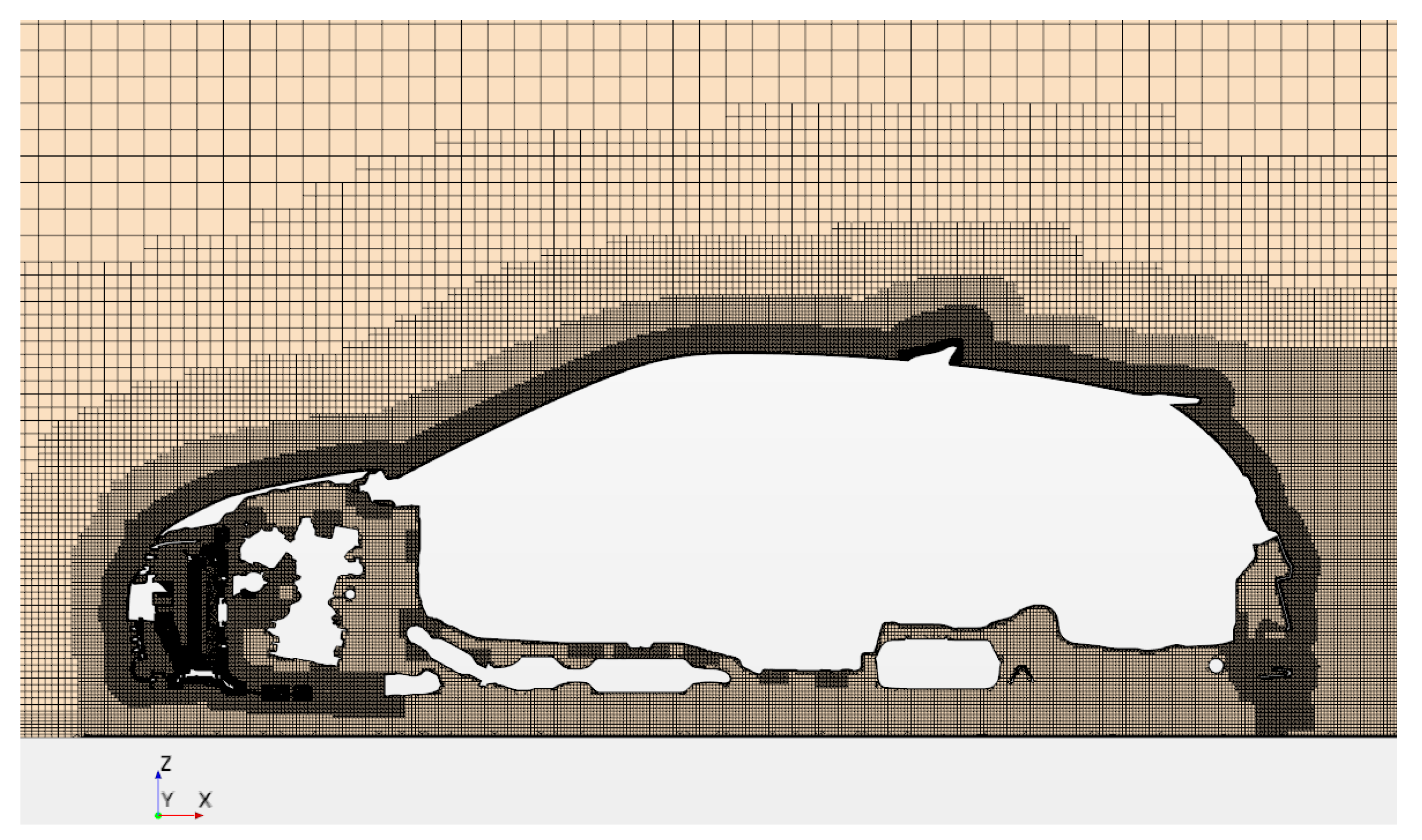
A mesh independence study was conducted first for the baseline case with the RKE and IDDES models to further eliminate the effects of the mesh on simulation results. For the RKE model, the fine mesh contained 100 million cells, which were generated by reducing the base size from 24 mm to 20 mm. A change of drag coefficient within 1% between 75 and 100 million cells was achieved in this process. However, for the IDDES model, simply reducing the base size will increase the computational cost dramatically, not only due to the increased cell number, but also due to the smaller time step resulting from reducing the core mesh size close to the vehicle. Thus, a different strategy, where only the cells in the wake region and underbody area were halved, was used to refine the mesh for the IDDES model. As suggested by [43], the recommended mesh size in the detached flow regions for a DES-type simulation should be close to the Taylor microscale given by $\lambda ={15}^{1/2}{A}^{-1/2}{R}_l^{-1/2}l$, where A is an undetermined constant set to be 0.5, l is the bulk integral scale (taken as the vehicle length, L), and $R_l$ the integral scale Reynolds number (here taken as the Reynolds number based on the free-stream velocity and vehicle overall length L). For the Reynolds number used in this study, the Taylor microscale $\lambda$ was estimated to be 7.9 mm. Therefore, the mesh strategy used to refine the IDDES case with a mesh size of 6 mm in the wake region and underbody was reasonably fine enough. The fine mesh of the IDDES model (shortened to IDDES fine in this study) contained 87 million cells by using this strategy. Further to eliminate the numerical uncertainty, the IDDES fine case was run with a CFL number of 0.5. It was found that the change of drag coefficient was within 1%; thus, the coarser mesh with a CFL number of one is sufficient enough for performing the intended investigations.

3.1. Drag and Lift Forces

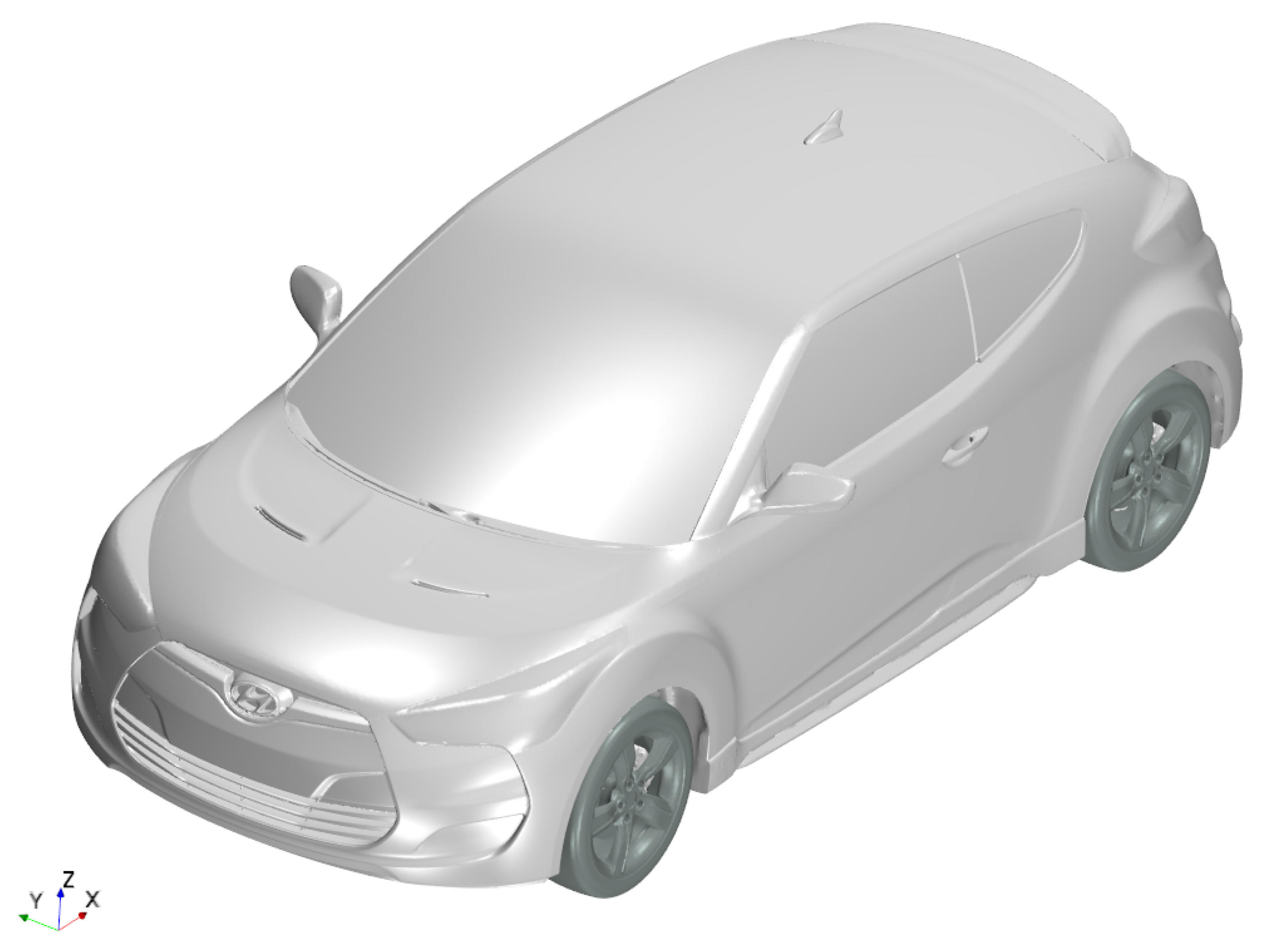
Due to the proprietary nature of the data, the drag coefficient values presented in this paper were normalized using an arbitrary reference area, such that the baseline car $C_D$ obtained from the RKE model matched with the one available in the public domain. Data downloaded from the website Edmunds.com,“features & specs 2014 Hyundai Veloster”, https://www.edmunds.com/hyundai/veloster/2014/features-specs/, accessed 19 June 2017, indicates that the drag coefficient of the 2014 model Hyundai Veloster is 0.320. Thus, the $C_D$ for the baseline case obtained from the RKE model was set to 0.320, and the predictions from all other approaches were nominalized accordingly.

Table 1. Percent deviation of $C_D$ predictions from the experimental data for the baseline vehicle model. RKE, Realizable $k-\epsilon$; AKN, Abe–Kondoh–Nagano; IDDES, Improved Delayed Detached Eddy Simulation.

$\%{\mathit{C}}_{\mathit{D}}$ Deviation	RKE	AKN	V2F	SST	DDES	IDDES	IDDES Fine
Case 1	1.3%	13.8%	10.0%	12.9%	11.5%	10.9%	10.8%

shows the percent deviation of the predicted $C_D$ values from the wind-tunnel test data for all investigated models; the data presented in this table correspond to the baseline vehicle model. Firstly, it can be seen that $C_D$ prediction from the RKE agreed very well with the experimental data. However, all other models predicted significantly higher drag coefficient, with the highest $C_D$ value coming from the AKN model. Unfortunately, while both the DDES and IDDES models, which apply the RANS SST model in the boundary layers, predicted a slightly better drag coefficient compared with that of the SST model, they failed to predict well-correlated $C_D$ values. Furthermore, for the DES models, while the $C_D$ prediction of the IDDES was slightly better than that of the DDES, the IDDES model with a fine mesh produced negligible improvement. The fact that even the IDDES fine case failed to predict well correlated $C_D$ values indicates the monumental challenge that is still encountered by the CFD simulation of automotive flows. Although the RKE model predicted a significantly better $C_D$ value than all other investigated models, it should be cautioned that this does not suggest the superior performance of the RKE model. For the RANS and DES models, the drag prediction may contain error cancellation of flow fields in different regions around the vehicle.

Table 2. Drag and lift coefficients for all models.

Case #	Model	${\mathit{C}}_{\mathit{D}}$	${\mathit{C}}_{\mathit{L}}$	${\mathit{C}}_{\mathit{L}}/{\mathit{C}}_{\mathit{D}}$	${\mathit{C}}_{\mathit{LF}}$	${\mathit{C}}_{\mathit{LR}}$	%Front
Case 1	RKE	0.320	0.098	0.305	−0.013	0.111	−13.2%
	AKN	0.360	0.096	0.267	−0.035	0.132	−36.5%
	V2F	0.348	0.129	0.371	−0.015	0.144	−11.4%
	SST	0.357	0.096	0.269	−0.033	0.130	−34.6%
	DDES	0.352	0.084	0.238	−0.041	0.126	−49.5%
	IDDES	0.350	0.060	0.171	−0.045	0.106	−75.4%
	IDDES Fine	0.350	0.072	0.206	−0.058	0.135	−80.8%
Case 2	RKE	0.290	0.073	0.251	−0.021	0.122	−29.1%
	AKN	0.331	0.050	0.150	−0.046	0.126	−92.6%
	V2F	0.322	0.065	0.201	−0.042	0.136	−65.7%
	SST	0.337	0.086	0.255	−0.037	0.152	−43.0%
	DDES	0.350	0.080	0.226	−0.077	0.157	−97.7%
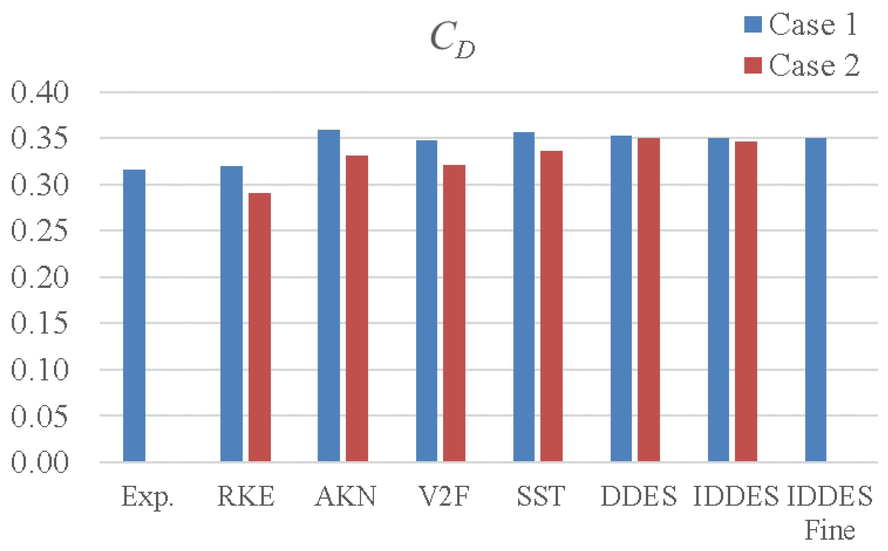
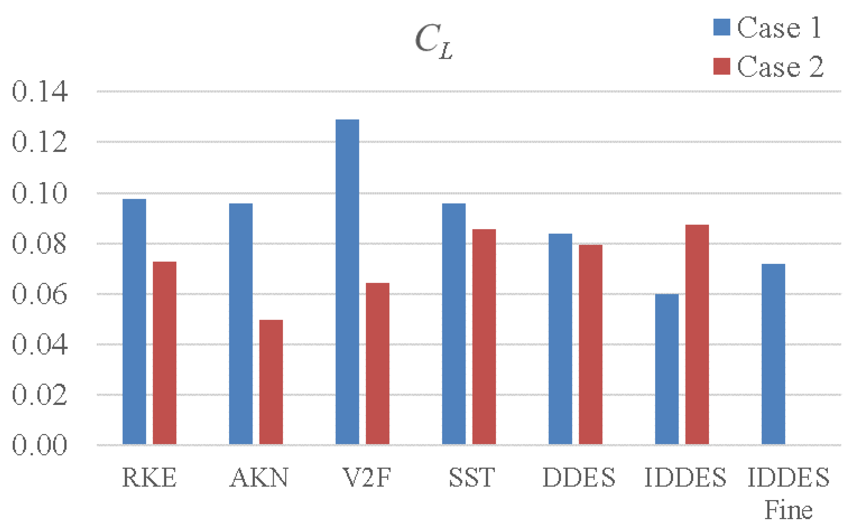
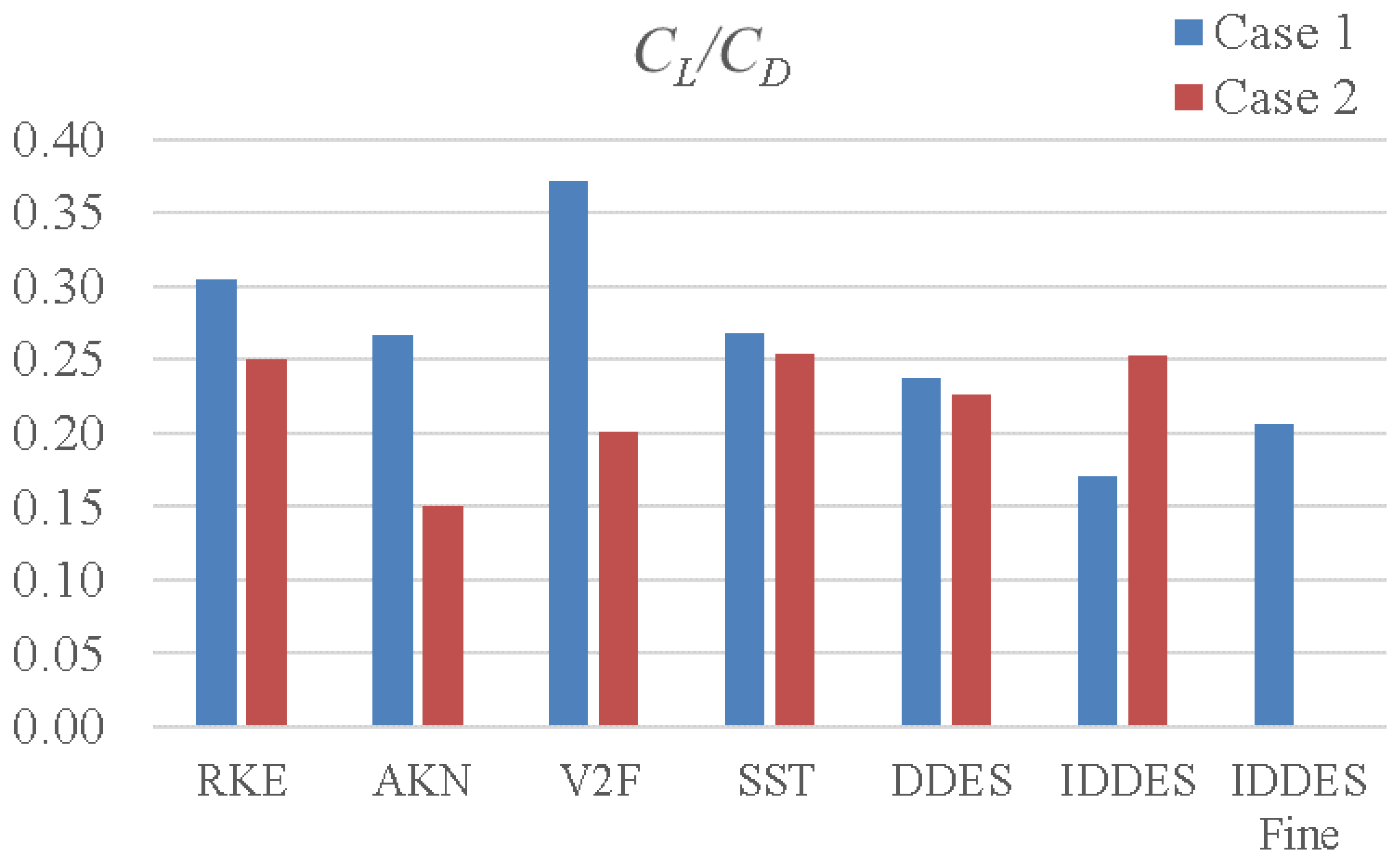
	IDDES	0.347	0.088	0.253	−0.072	0.160	−82.1%

summarizes drag and lift coefficients corresponding to both vehicle configurations as obtained from the studied turbulence models. These include the coefficients of drag, total lift, front and rear lift, and the front to total lift ratio, known as the lift balance or percent front. Data presented in Table 2 are graphically summarized in Figure 7, Figure 8 and Figure 9 to illustrate the predictive differences between all models in terms of drag, lift, and percent front. It can be seen that the RKE model predicted significantly smaller $C_D$ values for both cases compared to the other models. For instance, the RKE predicted a 11.1% less $C_D$ value than the AKN for Case 1 and a 17.1% smaller $C_D$ value than the DDES model for Case 2. Moreover, while all models predicted a higher $C_D$ value for the baseline case than that for the air-duct case, compared to the RANS predictions, the two DES variants predicted a much smaller difference between the two cases; see

Table 3. Delta drag and lift coefficients between Case 1 and Case 2 for all models.

Model	$\mathsf{\Delta }{\mathit{C}}_{\mathit{D}}$	$\mathsf{\Delta }{\mathit{C}}_{\mathit{L}}$	$\mathsf{\Delta }{\mathit{C}}_{\mathit{L}}/{\mathit{C}}_{\mathit{D}}$	$\mathsf{\Delta }{\mathit{C}}_{\mathit{LF}}$	$\mathsf{\Delta }{\mathit{C}}_{\mathit{LR}}$	$\mathsf{\Delta }$%Front
RKE	0.030	0.025	0.055	0.008	−0.011	15.9%
AKN	0.029	0.046	0.116	0.011	0.006	56.1%
V2F	0.026	0.065	0.171	0.028	0.007	54.3%
SST	0.020	0.010	0.014	0.004	−0.022	8.4%
DDES	0.002	0.005	0.012	0.036	−0.030	48.2%
IDDES	0.003	−0.028	−0.082	0.027	−0.053	6.7%

. For instance, while the IDDES predicted a $\Delta C_D$ of three counts between the two car configurations, the RKE model predicted a 30 count difference. While the variation of $\Delta C_D$ predictions between the RANS was within $\pm 5$ counts, the spread of $\Delta C_L$ predictions was much larger; note that, for any force coefficient $C_F$, $\Delta C_F$ is defined as the $C_F$ value from Case 1 minus the corresponding value from Case 2. Clearly, the predictive disagreements between the RANS models were most visible with the front lift ratio. Further, comparing the two IDDES simulations with different mesh strategies for the baseline case, while there was no difference in $C_D$ prediction, a noticeable discrepancy can be seen in $C_L$ prediction. In short, for all the turbulence models and mesh strategies studied, the prediction of drag was more consistent than that of lift. Moreover, even for industrial automotive flows that feature complex geometry and exhibit massive separations, a certain model could predict the $C_D$ value that correlates very well with the experimental data.

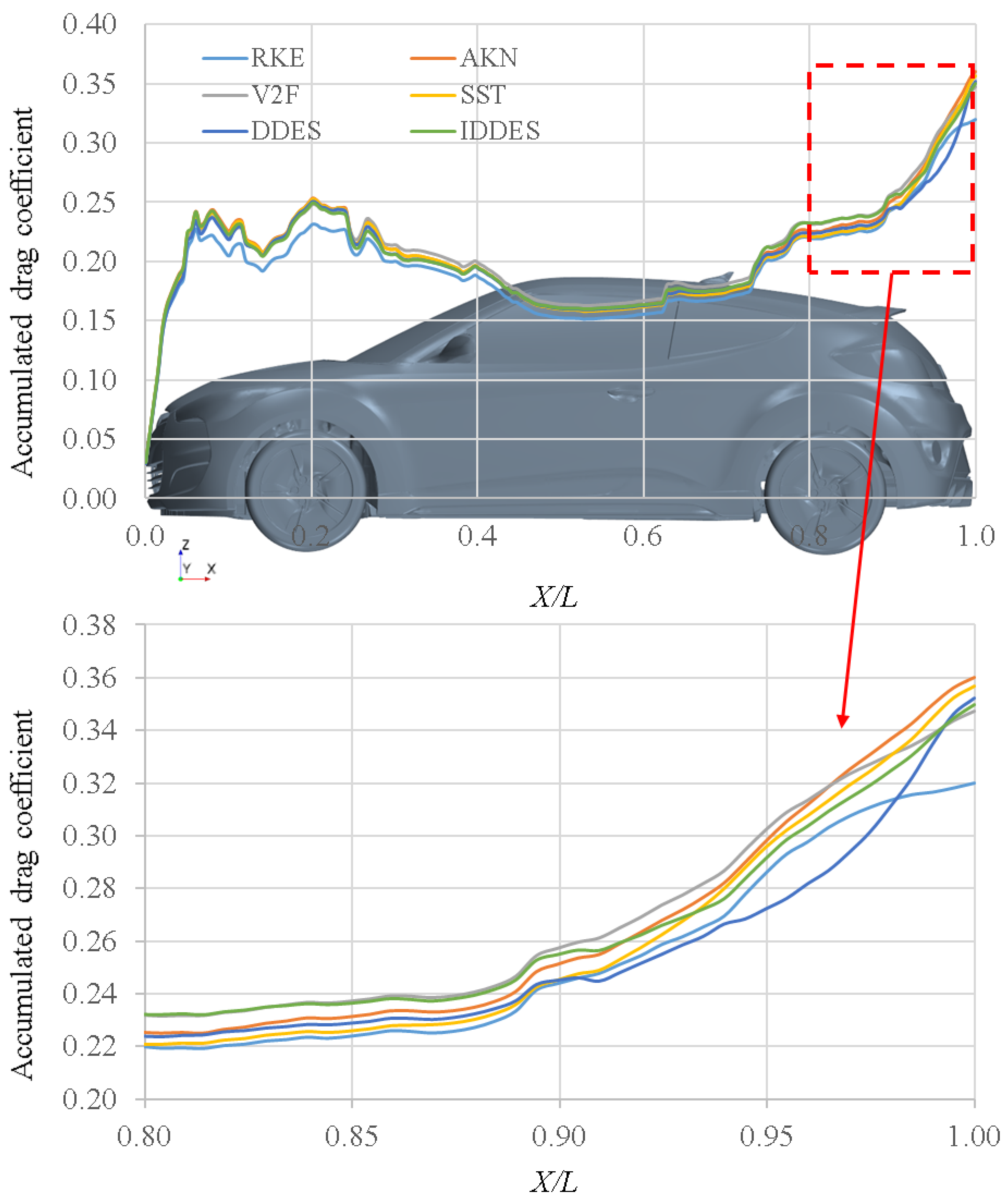
The accumulated drag coefficients along the vehicle centerline for the baseline case as obtained from all turbulence models are shown in Figure 10. It can be seen, firstly, that before the airflow passed through the CRFM ($0<X/L<0.06$), all the models predicted almost identical results; then, in the underhood region from the CRFM to the cowl area ($0.06<X/L<0.25$), the RKE predicted a significantly lower drag value compared to all other models. Nevertheless, the results from the RKE in this region still followed the same trend as all other models. Further, all the models predicted almost identical trends, though with different magnitudes, in the region between the cowl area and the rear spoiler where the flow was mostly attached ($0.25<X/L<0.85$). However, at the rear end of the vehicle, the predictions from all the models started to diverge from each other significantly, especially that of the DDES and the RKE. In short, for the vehicle model used in this study, all the turbulence models investigated could predict consistent results even in the underhood compartment where the flow was featured with separations and complex interactions between the cooling airflow and underbody airflow. However, no consistent results between all the models were observed for the prediction of the wake region where massive separation occurred.

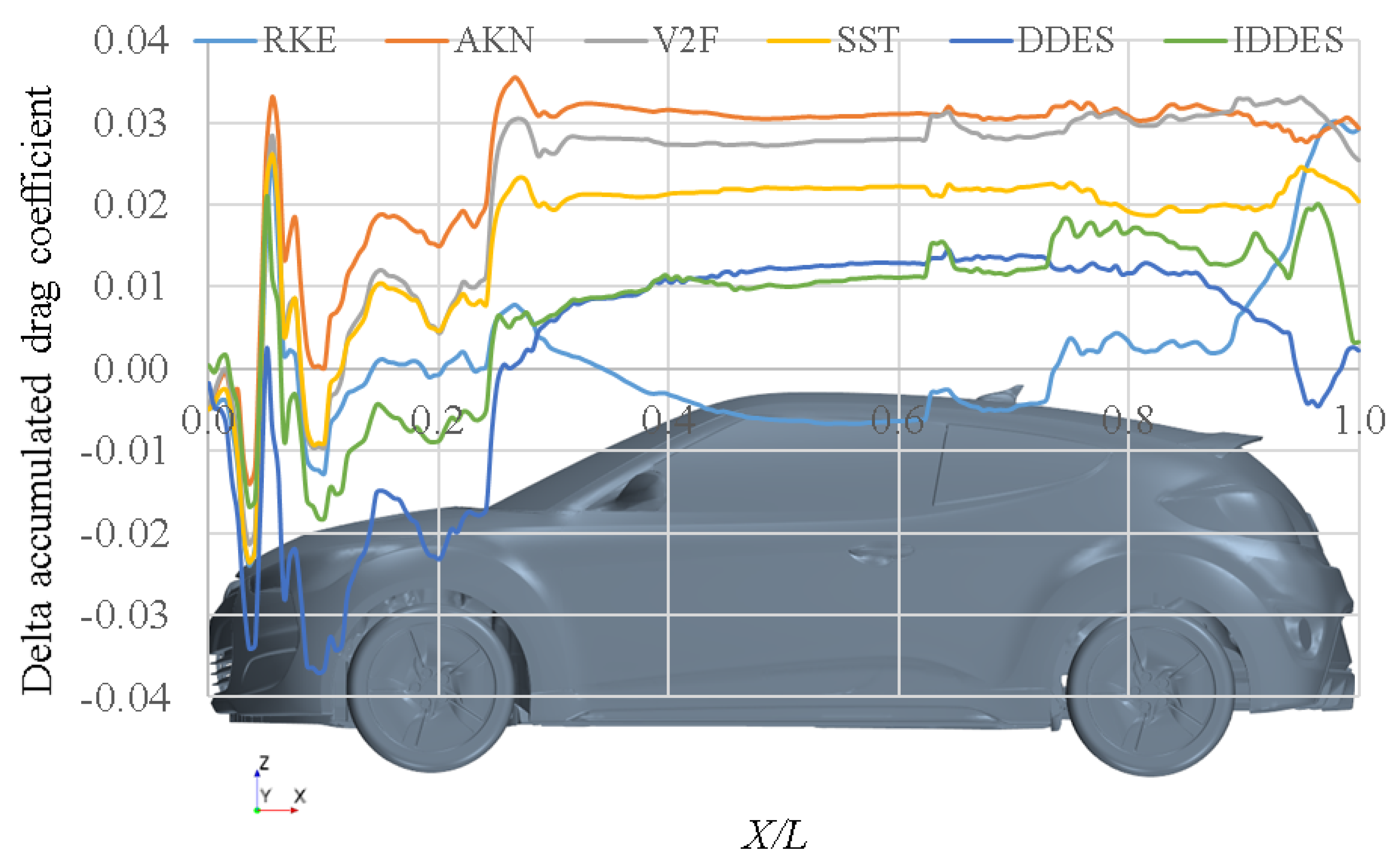
The delta accumulated drag coefficients (between Case 1 and Case 2 vehicle configurations) obtained using all turbulence models are shown in Figure 11. Firstly, it is not surprising to observe significant prediction fluctuations in the front part of the vehicle since the only difference between the two vehicle configurations was the front end geometry. For this part of the vehicle, although all turbulence models predicted similar trends, noticeable differences in magnitude indicated a high sensitivity of the $C_D$ prediction to the choice of turbulence models. Further, the noticeable fluctuations in the rear end of the vehicle, especially for the RKE, DDES, and IDDES models, highlighted the strong influence of the predictions of upstream flow on the downstream flow. Moreover, the prediction trend of the RKE model differed significantly from all other models in two areas: the windshield and the rear end. The causes of prediction differences will be qualitatively and quantitatively analyzed in the following sections.

3.2. Pressure and Velocity Fields

3.2.1. Baseline Case

As stated in the previous section, the front and rear ends of the vehicle contributed most to the $C_D$ difference for all the turbulence models studied. To better analyze the $C_D$ prediction differences for all the models, pressure and velocity fields at the front and rear ends of the vehicle were investigated.

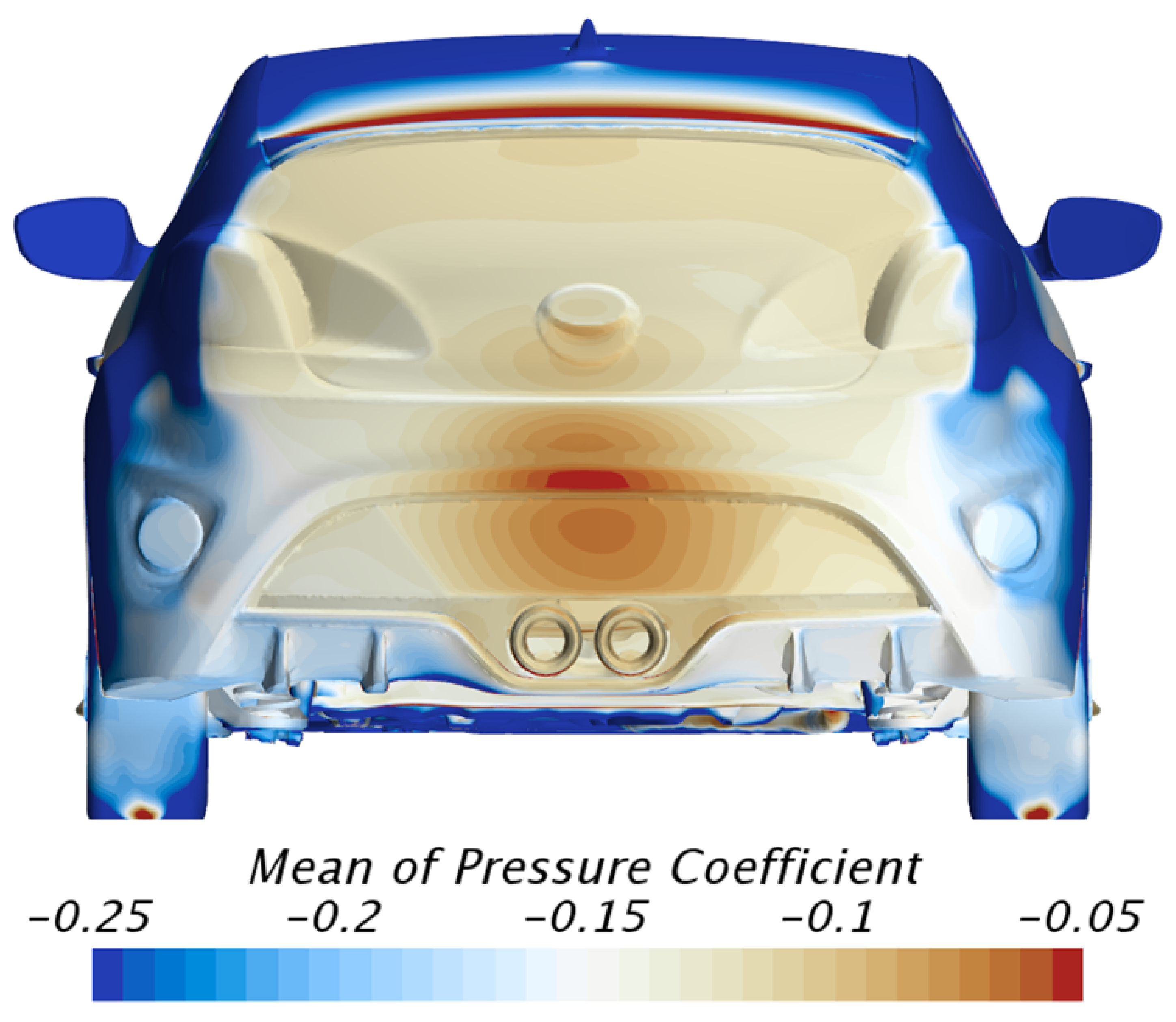
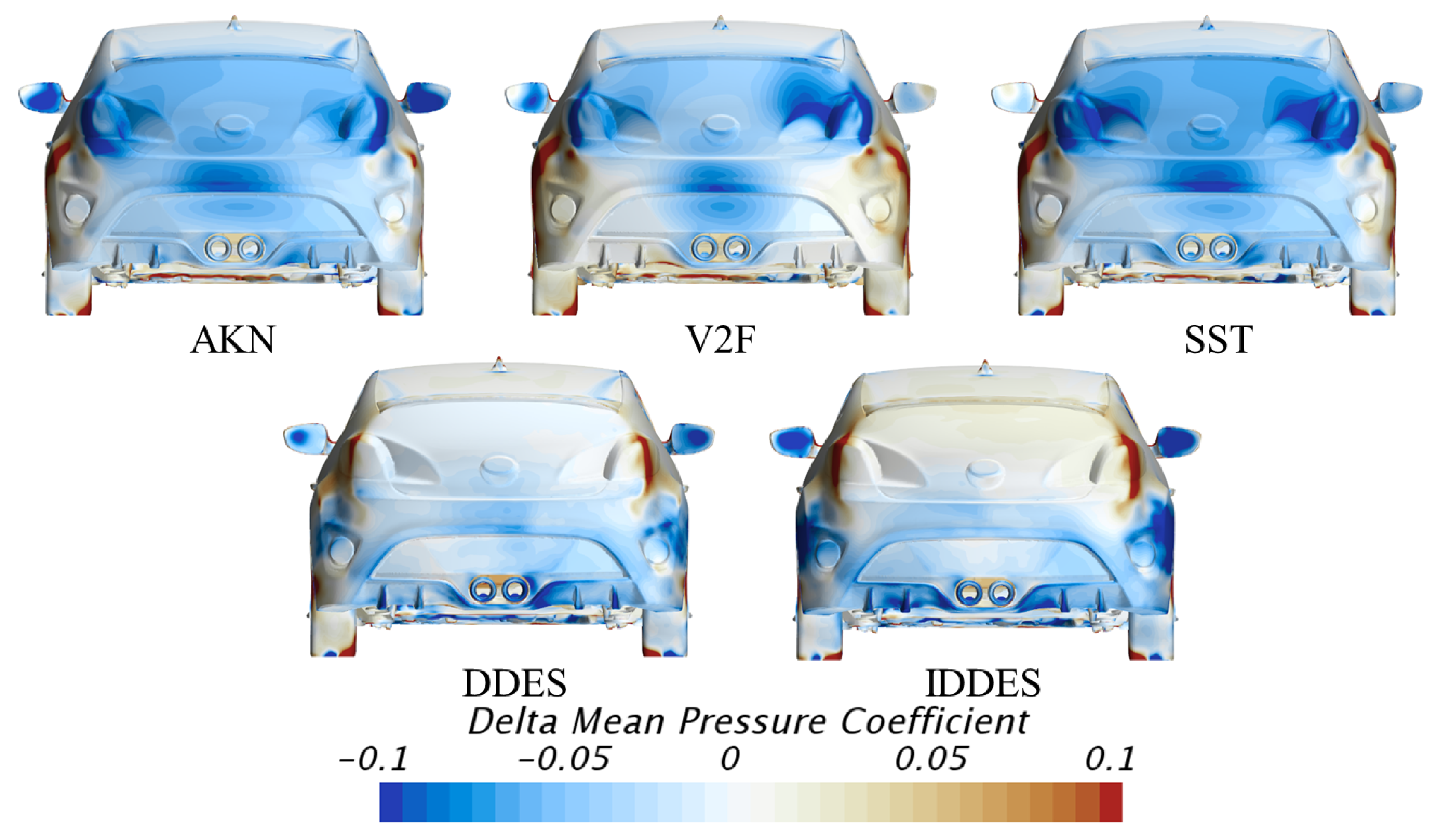
For the baseline case, since the RKE predicted a significantly lower $C_D$ value, the pressure coefficient on the back of the vehicle from this model is shown first in Figure 12. It can be seen that the most noticeable higher pressure area was right above the exhaust pipe. This area was the saddle of attachment of the wake flow as supported by the streamline structure in Figure 13 for the RKE model (Top left). To better illustrate the differences between the RKE and other models for the baseline case flow prediction, contours of $\Delta C_P$, where $\Delta C_P$ represents $C_P$ from a model relative to $C_P$ obtained from the RKE, are shown in Figure 14. Firstly, all other models predicted overall lower pressure when compared with that of the RKE, especially the three RANS models. This is consistent with the results of accumulated drag as shown in Figure 10. More specifically, the $\Delta C_P$ predicted by the AKN model might be explained by the key differences between the RKE and the AKN model on how these two models solve the viscosity-dominated near-wall flow regions. The RKE model used a two-layer approach (the Star-CCM+ implementation of this approach was after [34]), and the AKN model adopted a low-Reynolds number approach with the introduction of the Kolmogorov velocity scale, instead of the friction velocity, to account for the near-wall and low-Reynolds number effects in both attached and detached flow. On the other hand, both of V2F and SST models can resolve down to the viscosity-dominated near-wall regions. Thus, more evident prediction differences in certain areas, such as the area around the right taillight and both sides of the vehicle, are expected. Further, the delta pressure distributions predicted by the two DES variants showed a completely different pattern compared to those from the other three RANS models. Interestingly, they both predicted less discrepancies against that of the RKE model, with slightly higher pressure on the upper part, but lower pressure on the lower part.

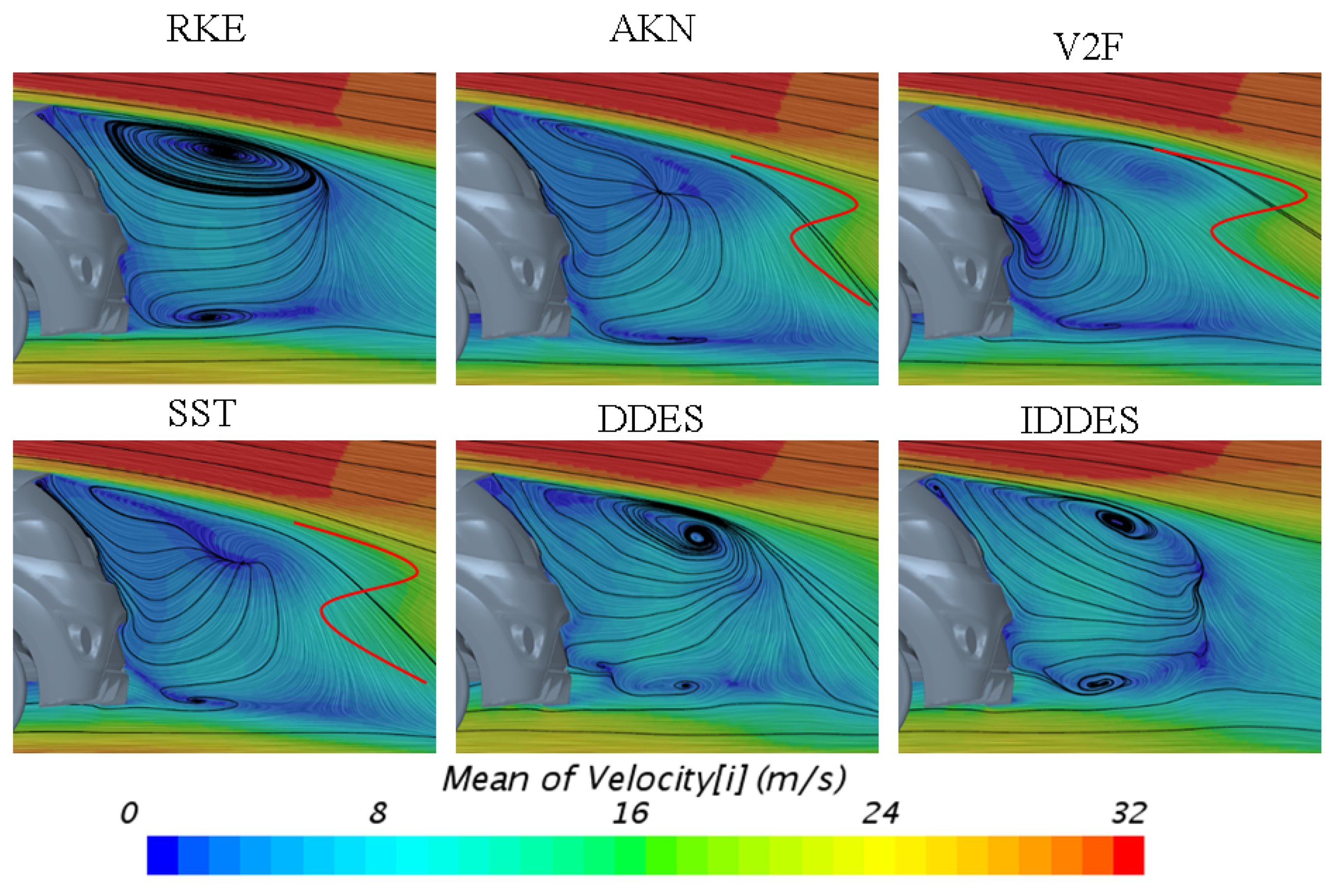
The vector scenes with constrained streamlines presented insights into the wake structure, as demonstrated in Figure 13. Firstly, the RKE model predicted two strong counter-rotating vortices with the saddle-like attachment area right above the exhaust pipes (see Figure 12). Secondly, compared to the RKE model, the other three RANS models predicted significantly different wake structures: (1) no counter-rotating vortices existed; (2) the lower vortex was much weaker and the saddle of attachment area at a lower location; (3) the wake area was much smaller (see the areas on the right of the red spline line in the corresponding images). On the other hand, again interestingly, two DES variants predicted a mostly similar wake structure as that of the RKE model, e.g., counter-rotating vortices, saddle of attachment location, and similar wake area. However, some differences can still be observed: (1) the top vortex core was at a further downstream location; (2) wake structures were more complex, especially as the DDES predicted a tertiary vortex near the exhaust pipes, and the IDDES predicted a tertiary vortex under the spoiler.

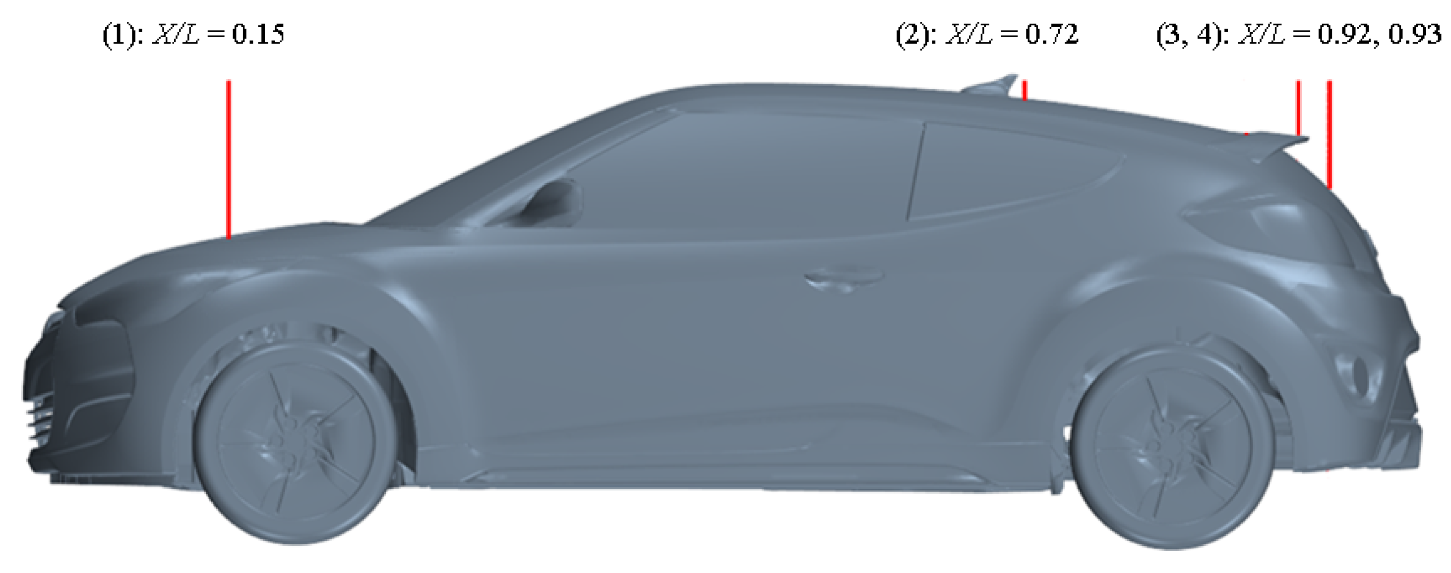
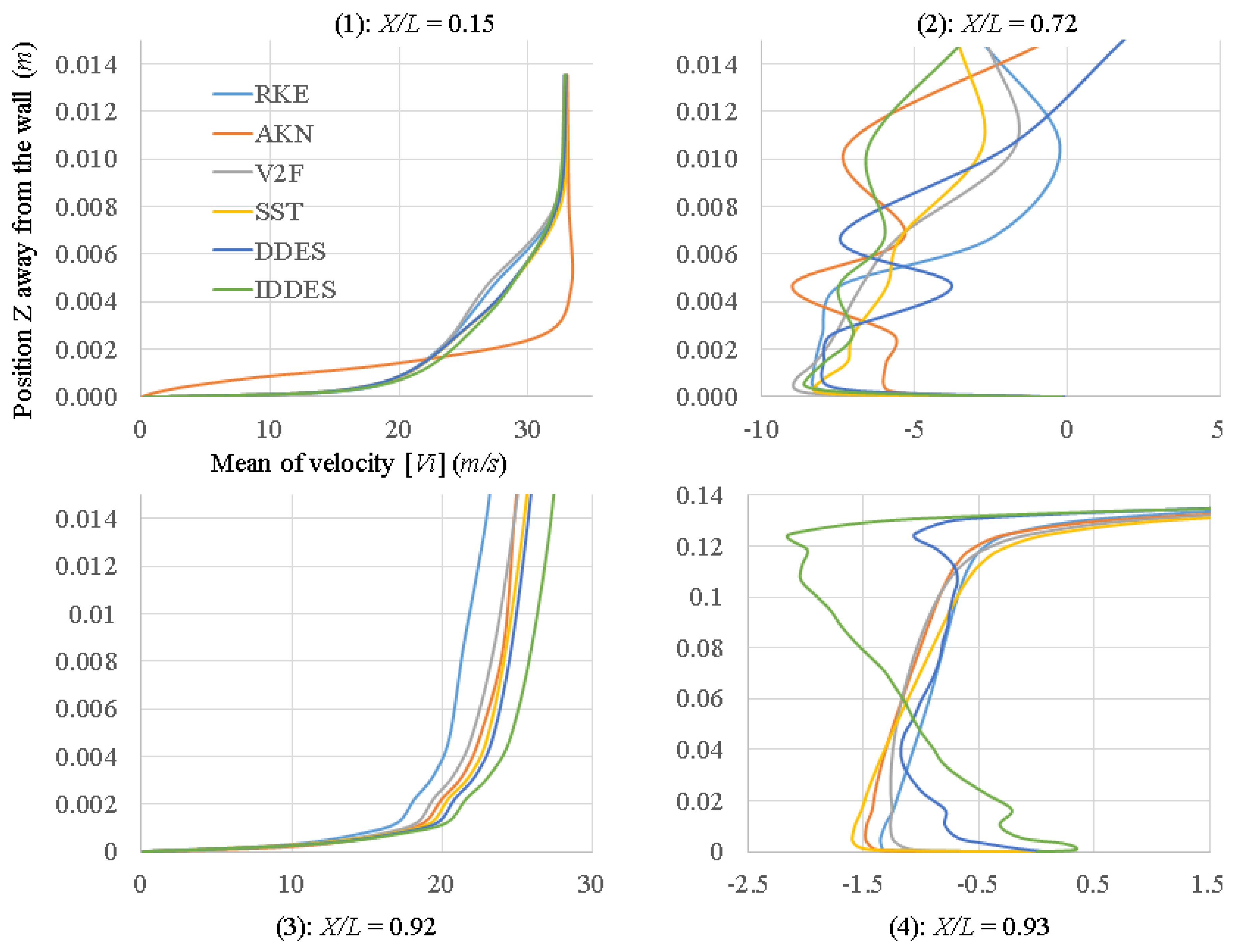
To further investigate the prediction differences between all the models studied, streamwise velocity profiles for the baseline case are shown at four selected locations. These lines are marked with red lines in Figure 15 and are located (1) on the hood, (2) behind the antenna, (3) on the rear end of the spoiler, and (4) on the rear glass. The velocity profiles are shown in Figure 16. It can be seen that, for Locations 1 and 3, where the flow was attached, similar trends can be observed in the predictions from all models except for the AKN model at Location 1 on the hood. At Location 3, right on the rear end of the spoiler, where the flow was mostly attached and fully turbulent, all the models showed similar predictions in the viscosity-dominated near-wall region. This implies that the wall treatments used by different models worked rather well in the attached flow region. However, above the viscosity-dominated region, the models studied start to show differences in terms of boundary layer growth. Clearly, the RKE showed the smallest boundary layer thickness, and the IDDES predicted the thickest boundary layer at Location 3. The unexpected streamwise velocity profile from the AKN at Location 1 looked quite suspicious, and indicated that the low-Reynolds number approach implemented in the AKN model may not work well even in the attached flow region. On the other hand, for Locations 2 and 4, which were in wake regions, all models studied differed from each other significantly. In short, for the models studied, while a consistent streamwise velocity profile could be observed in attached flow regions except for the AKN model, the significant different predictions of the streamwise velocity in the wake regions further showed a strong dependence of the turbulence models on the prediction of complex automotive flows.

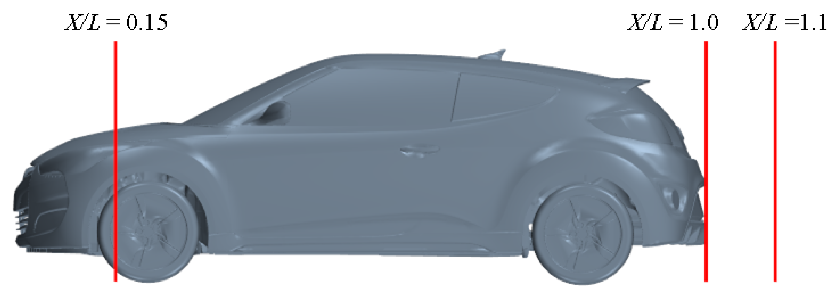
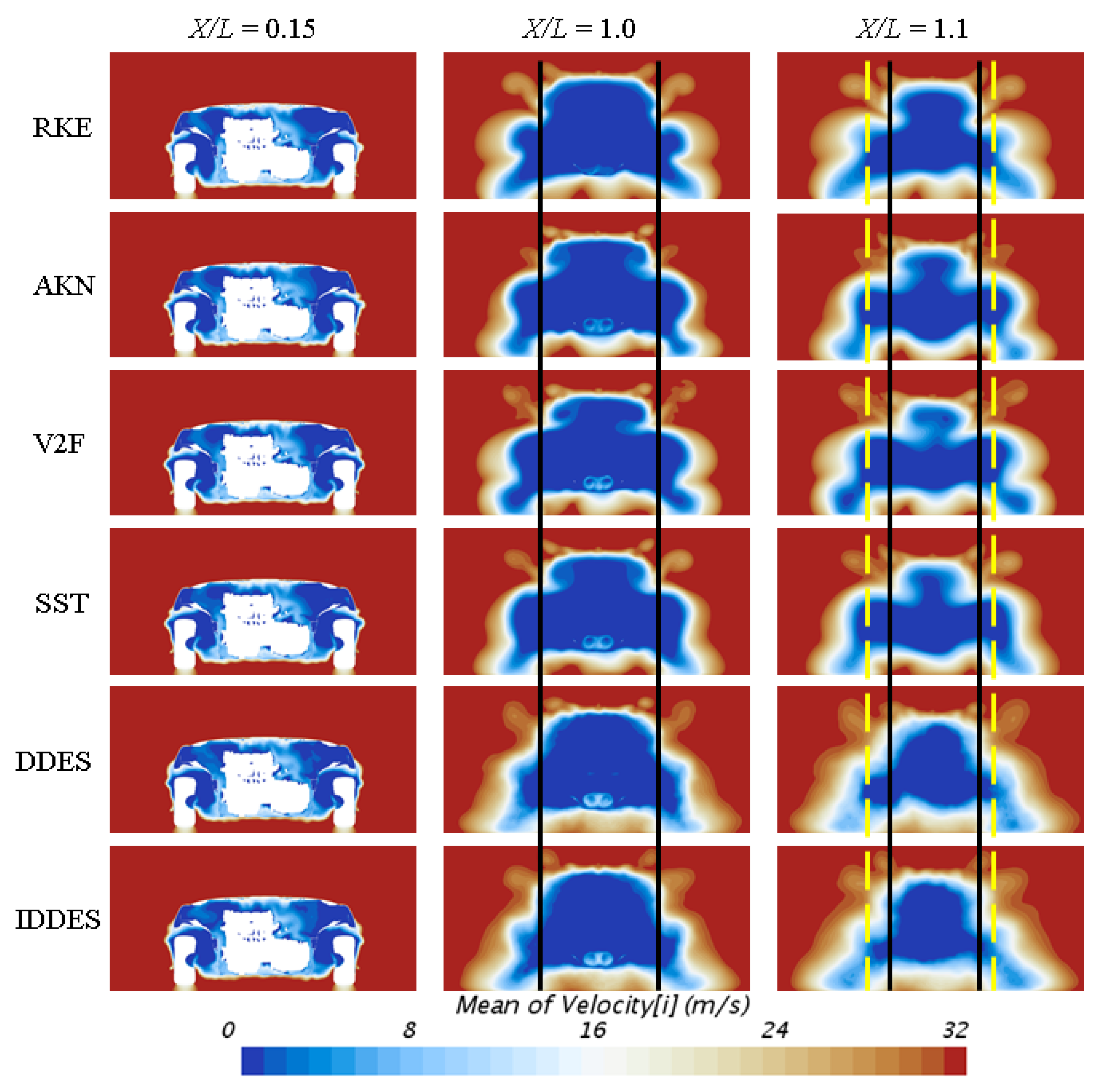
For the sake of a more comprehensive analysis of the flow fields, three plane sections were selected for flow visualizations. As shown in Figure 17, these planes are: (1) through the underhood area; (2) at the rear of the vehicle; (3) inside the wake region. Streamwise velocity scenes on these three selected plane sections from all models for the baseline case are shown in Figure 18. It can be seen that, on Plane 1 at $X/L=0.15$, all models predicted a similar streamwise velocity distribution. However, compared to the other three RANS models, the RKE model predicted a larger negative streamwise velocity area in the upper part of the wake region on planes $X/L=$ 1.0 1.1 (see the area bound by the black lines). Moreover, the RKE model predicted a smaller negative streamwise velocity area in the lower part of the wake region on plane $X/L=1.1$ (see the yellow dashed lines). Surprisingly, the predictions from the two DES variants were quite similar to that of the RKE model on both selected planes. The similarity of the streamwise velocity profile on these two planes between the predictions from the DES variants and the RKE model supports that the RKE model performed better than the other three RANS models for the baseline case. This can be further confirmed by the delta streamwise velocity against the IDDES fine model on these planes, as shown in Figure 19. It can be seen that the RKE predicted closer velocity profiles in the wake region to that of the IDDES fine model than the other three RANS models. Moreover, the IDDES case with the coarse mesh predicted very similar results as that from the fine mesh, which indicates that the coarse mesh was sufficient enough for this study.

3.2.2. Comparison between the Baseline Case and the Air-Duct Case

This section presents analyses of how the selected turbulence models predicted the flow differences between two car configurations. This was done by presenting delta values of pressure and velocity; delta pressure or velocity means the quantity for Case 2 (the air-duct case) subtracted from that of Case 1 (the baseline case).

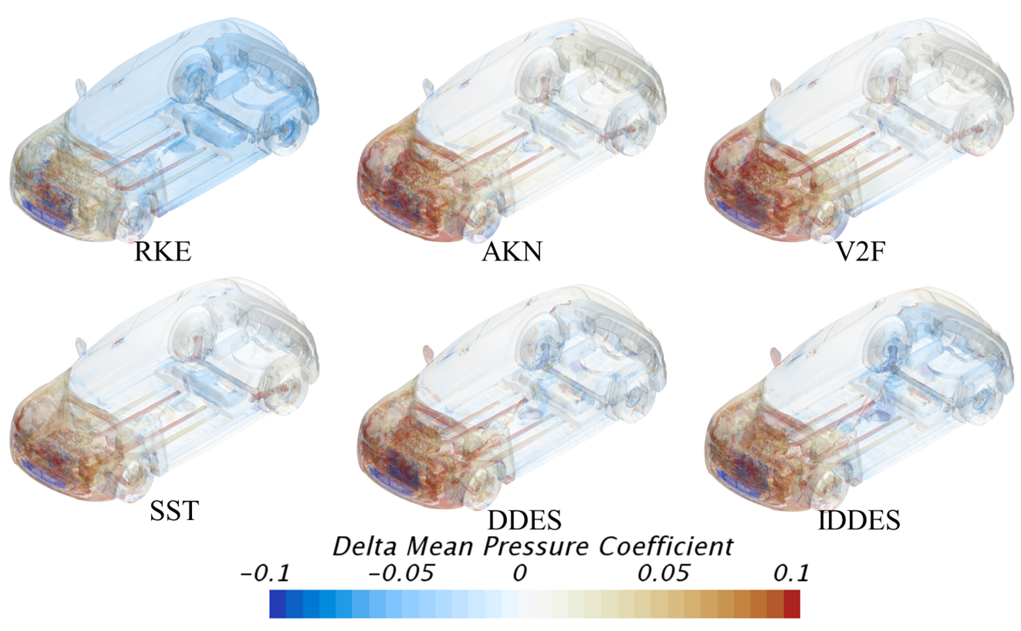
Scenes of delta pressure coefficient ($C_p$ of Case 2 relative to the baseline Case 1), as obtained from the selected models, are shown in Figure 20. Firstly, as expected, all the models predicted a higher pressure coefficient in the front end part of the vehicle for the baseline case, since the larger front grille opening in the baseline configuration will result in more airflow entering the underhood compartment. However, noticeable differences can be observed for the pressure distribution predictions on the rest of the car. In particular, the prediction from the RKE model differed significantly from that of all other models; the RKE model predicted noticeable lower pressure on the rest of the car. This is consistent with the delta accumulated drag plot discussed earlier in Figure 11. Further, the two DES variants predicted lower pressure on the rear bottom part of the vehicle. These observations indicate that the change of upstream geometry may result in noticeably different downstream predictions of the flow field depending on the choice of turbulence models.

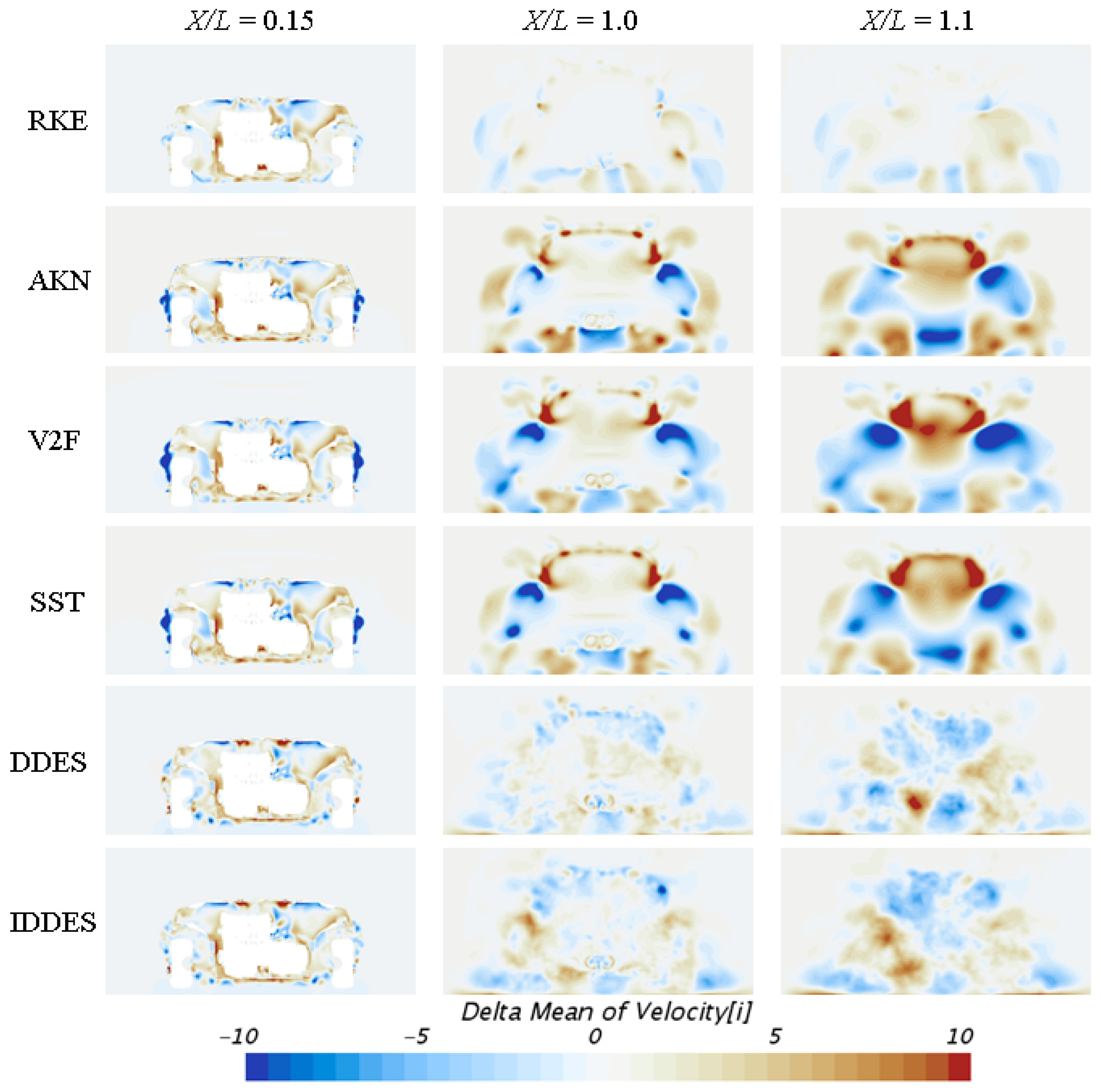
Scalar scenes of delta mean streamwise velocity (the mean streamwise velocity of Case 2 relative to the baseline Case 1), as obtained from the selected models, are shown in Figure 21; see Figure 17 for the location of these planes. The most significant differences in delta mean streamwise velocity at $X/L=0.15$ corresponded to RKE predictions near the far left and right sides. These two area denote the region of the flow most influenced by the tire rotation effects. This indicates that the prediction of flows subject to rotation was different for the RKE model compared to the rest RANS model. Surprisingly, the RKE deltas were much more aligned with the predictions from the scale-resolved DDES or IDDES models, which again strengthens the earlier argument that the RKE-based RANS approach produced a more realistic flow field compared to the other steady state RANS models for this particular vehicle geometry. Another interesting point is that the RKE model predicted larger delta pressure distributions on most part of the vehicle, as shown in Figure 20. Furthermore, the delta streamwise velocity on the two planes in the wake regions predicted by the RKE model was much smaller than that of the other three RANS models. On the other hand, the two DES variants predicted a slightly larger deviation than that of the RKE model, but much smaller than that of the other three RANS models.

4. Conclusions

This study presented a numerical evaluation of various commonly-used RANS models and hybrid RANS/LES models on a full-scale passenger vehicle with two different front-end configurations. The effect of turbulence modeling on the prediction of drag and lift forces, pressure, and velocity field were investigated. It was found that, firstly, the RKE model predicted a well-correlated $C_D$ value for the baseline case; however, all the models investigated still needed significant improvement in order to predict the lift values consistently. Secondly, despite the DES variants not showing superior performance over RANS models for predicting the absolute $C_D$ value, they were able to predict more complex flow structures with a higher fidelity. For example, in Figure 13, the DDES model predicted a tertiary vortex near the exhaust pipes, and the IDDES model predicted a tertiary vortex under the spoiler. The similarity of the streamwise velocity profile and turbulent kinetic energy distribution on the selected planes between the predictions from the RKE model and the DES variants supports that the RKE model performed better than the other three RANS models for the baseline case.

In summary, for automotive flows that feature complex geometry and exhibit massive separation, the success of CFD simulation still heavily relies on the choice of mesh strategy and turbulent models, which in turn depend on the experience of the engineer. RANS models might still be a good choice for the prediction of drag values due to their acceptable accuracy, low computational cost, and fast turnaround time. However, for applications that require predictions of the detailed flow features, such as aeroacoustic, soiling, and water management, the transient DES type approaches would be a better choice.

References

1. Ashton, N.; Revell, A. Comparison of RANS and DES Methods for the DrivAer Automotive Body; Technical Report, SAE Technical Paper; SAE: Warrendale, PA, USA, 2015. [Google Scholar]
2. Ashton, N.; West, A.; Lardeau, S.; Revell, A. Assessment of RANS and DES methods for realistic automotive models. Comput. Fluids 2016, 128, 1–15. [Google Scholar] [CrossRef] [Green Version]
3. Guilmineau, E.; Deng, G.; Leroyer, A.; Queutey, P.; Visonneau, M.; Wackers, J. Assessment of hybrid RANS-LES formulations for flow simulation around the Ahmed body. Comput. Fluids 2017, 176, 302–319. [Google Scholar] [CrossRef]
4. Fu, C.; Bounds, C.P.; Selent, C.; Uddin, M. Turbulence modeling effects on the aerodynamic characterizations of a NASCAR Generation 6 race car subject to yaw and pitch changes. Proc. Inst. of Mech. Eng. Part D J. Automob. Eng. 2019. [Google Scholar] [CrossRef]
5. Shur, M.; Spalart, P.; Strelets, M.; Travin, A. Detached-eddy simulation of an airfoil at high angle of attack. In Engineering Turbulence Modelling and Experiments 4; Elsevier: Amsterdam, The Netherlands, 1999; pp. 669–678. [Google Scholar]
6. Spalart, P.R. Young-Person’s Guide to Detached-Eddy simulation Grids; Technical Report; NASA Langley Research Center: Hampton, VA, USA, 2001. [Google Scholar]
7. Spalart, P.R.; Deck, S.; Shur, M.L.; Squires, K.D.; Strelets, M.K.; Travin, A. A new version of detached-eddy simulation, resistant to ambiguous grid densities. Theor. Comput. Fluid Dynam. 2006, 20, 181. [Google Scholar] [CrossRef]
8. Shur, M.L.; Spalart, P.R.; Strelets, M.K.; Travin, A.K. A hybrid RANS-LES approach with delayed-DES and wall-modeled LES capabilities. Int. J. Heat Fluid Flow 2008, 29, 1638–1649. [Google Scholar] [CrossRef]
9. Ahmed, S.; Ramm, G.; Faltin, G. Some Salient Features of the Time-Averaged Ground Vehicle Wake; Technical Report, SAE Technical Paper; SAE: Warrendale, PA, USA, 1984. [Google Scholar]
10. Heft, A.; Indinger, T.; Adams, N. Investigation of unsteady flow structures in the wake of a realistic generic car model. In Proceedings of the 29th AIAA Applied Aerodynamics Conference, Honolulu, HI, USA, 27–30 June 2011; p. 3669. [Google Scholar]
11. Han, T. Computational analysis of three-dimensional turbulent flow around a bluff body in ground proximity. AIAA J. 1989, 27, 1213–1219. [Google Scholar] [CrossRef]
12. Gilliéron, P.; Chometon, F. Modelling of stationary three-dimensional separated air flows around an Ahmed reference model. In ESAIM: Proceedings; EDP Sciences: Les Ulis, France, 1999; Volume 7, pp. 173–182. [Google Scholar]
13. Guilmineau, E. Computational study of flow around a simplified car body. J. Wind Eng. Ind. Aerodyn. 2008, 96, 1207–1217. [Google Scholar] [CrossRef]
14. Ashton, N.; Revell, A. Key factors in the use of DDES for the flow around a simplified car. Int. J. Heat Fluid Flow 2015, 54, 236–249. [Google Scholar] [CrossRef]
15. Krajnović, S.; Davidson, L. Large-Eddy Simulation of the Flow around Simplified Car Model; Technical Report, SAE Technical Paper; SAE: Warrendale, PA, USA, 2004. [Google Scholar]
16. Minguez, M.; Pasquetti, R.; Serre, E. High-order large-eddy simulation of flow over the “Ahmed body” car model. Phys. Fluids 2008, 20, 095101. [Google Scholar] [CrossRef]
17. Heft, A.I.; Indinger, T.; Adams, N.A. Introduction of a New Realistic Generic Car Model for Aerodynamic Investigations; Technical Report, SAE Technical Paper; SAE: Warrendale, PA, USA, 2012. [Google Scholar]
18. Heft, A.I.; Indinger, T.; Adams, N.A. Experimental and numerical investigation of the DrivAer model. In ASME 2012 Fluids Engineering Division Summer Meeting Collocated with the ASME 2012 Heat Transfer Summer Conference and the ASME 2012 10th International Conference on Nanochannels, Microchannels, and Minichannels; American Society of Mechanical Engineers: New York, NY, USA, 2012; pp. 41–51. [Google Scholar]
19. Peters, B.C.; Uddin, M.; Bain, J.; Curley, A.; Henry, M. Simulating DrivAer with Structured Finite Difference Overset Grids; Technical Report, SAE Technical Paper; SAE: Warrendale, PA, USA, 2015. [Google Scholar]
20. Guilmineau, E. Numerical simulations of flow around a realistic generic car model. SAE Int. J. Passeng. Cars Mech. Syst. 2014, 7, 646–653. [Google Scholar] [CrossRef]
21. Jakirlic, S.; Kutej, L.; Basara, B.; Tropea, C. Computational study of the aerodynamics of a realistic car model by means of RANS and hybrid RANS/LES approaches. SAE Int. J. Passeng. Cars Mech. Syst. 2014, 7, 559–574. [Google Scholar] [CrossRef]
22. Fu, C.; Uddin, M.; Robinson, C.; Guzman, A.; Bailey, D. Turbulence Models and Model Closure Coefficients Sensitivity of NASCAR Racecar RANS CFD Aerodynamic Predictions. SAE Int. J. Passeng. Cars Mech. Syst. 2017, 10, 330–344. [Google Scholar] [CrossRef]
23. Argyropoulos, C.; Markatos, N. Recent advances on the numerical modelling of turbulent flows. Appl. Math. Model. 2015, 39, 693–732. [Google Scholar] [CrossRef]
24. Shih, T.H.; Liou, W.W.; Shabbir, A.; Yang, Z.; Zhu, J. A new k-ϵ eddy viscosity model for high Reynolds number turbulent flows. Comput. Fluids 1995, 24, 227–238. [Google Scholar] [CrossRef]
25. Abe, K.; Kondoh, T.; Nagano, Y. A new turbulence model for predicting fluid flow and heat transfer in separating and reattaching flows—I. Flow field calculations. Int. J. Heat Mass Transf. 1994, 37, 139–151. [Google Scholar] [CrossRef]
26. Durbin, P.A. Near-wall turbulence closure modeling without “damping functions”. Theor. Comput. Fluid Dynam. 1991, 3, 1–13. [Google Scholar]
27. Menter, F.R. Two-equation eddy-viscosity turbulence models for engineering applications. AIAA J. 1994, 32, 1598–1605. [Google Scholar] [CrossRef] [Green Version]
28. Menter, F.R. Review of the shear-stress transport turbulence model experience from an industrial perspective. Int. J. Comput. Fluid Dynam. 2009, 23, 305–316. [Google Scholar] [CrossRef]
29. Gritskevich, M.S.; Garbaruk, A.V.; Schütze, J.; Menter, F.R. Development of DDES and IDDES formulations for the k-ω shear stress transport model. Flow Turbul. Combust. 2012, 88, 431–449. [Google Scholar] [CrossRef]
30. Jones, W.P.; Launder, B.E. The prediction of laminarization with a two-equation model of turbulence. Int. J. Heat Mass Transf. 1972, 15, 301–314. [Google Scholar] [CrossRef]
31. Launder, B.E.; Sharma, B.I. Application of the energy-dissipation model of turbulence to the calculation of flow near a spinning disc. Lett. Heat Mass Transf. 1974, 1, 131–137. [Google Scholar] [CrossRef]
32. Durbin, P. On the k-ϵ stagnation point anomaly. Int. J. Heat Fluid Flow 1996, 17, 89–90. [Google Scholar] [CrossRef]
33. Launder, B.E.; Kato, M. Modeling flow-induced oscillations in turbulent flow around a square cylinder. In Proceedings of the ASME Fluid Engineering Conference, Washington, DC, USA, 20–24 June 1993; Volume 20. [Google Scholar]
34. Wolfshtein, M. The velocity and temperature distribution in one-dimensional flow with turbulence augmentation and pressure gradient. Int. J. Heat Mass Transf. 1969, 12, 301–318. [Google Scholar] [CrossRef]
35. Davidson, L.; Nielsen, P.V.; Sveningsson, A. Modifications of the V2 Model for Computing the Flow in a 3D Wall Jet. In Proceedings of the International Symposium on Turbulence, Heat and Mass Transfer, Antalya, Turkey, 12–17 October 2003. [Google Scholar]
36. Giannuzzi, M. Low Reynolds turbulence model CFD simulation for complex electronic system: An industrial point of view. J. Phys. Conf. Ser. 2014, 525, 012002. [Google Scholar] [CrossRef]
37. Durbin, P.A. Separated flow computations with the k-epsilon-v-squared model. AIAA J. 1995, 33, 659–664. [Google Scholar] [CrossRef]
38. Wilcox, D.C. Reassessment of the scale-determining equation for advanced turbulence models. AIAA J. 1988, 26, 1299–1310. [Google Scholar] [CrossRef]
39. Wilcox, D.C. Formulation of the kw turbulence model revisited. AIAA J. 2008, 46, 2823–2838. [Google Scholar] [CrossRef]
40. Spalart, P.R. Comments on the feasibility of LES for wings, and on a hybrid RANS/LES approach. In Proceedings of the First AFOSR International Conference on DNS/LES; Greyden Press: Dayton, OH, USA, 1997. [Google Scholar]
41. Menter, F.R.; Kuntz, M.; Langtry, R. Ten years of industrial experience with the SST turbulence model. Turbul. Heat Mass Transf. 2003, 4, 625–632. [Google Scholar]
42. Zhang, C.; Uddin, M.; Song, X.; Fu, C.; Foster, L. Simultaneous Improvement of Vehicle Under-Hood Airflow and Cooling Drag Using 3D CFD Simulation. In Proceedings of the SAE 2016 World Congress and Exhibition, Detroit, MI, USA, 12–14 April 2016; SAE International: Warrendale, PA, USA, 2016. [Google Scholar] [CrossRef]
43. Howard, R.; Pourquie, M. Large eddy simulation of an Ahmed reference model. J. Turbul. 2002, 3, 1–18. [Google Scholar] [CrossRef]
Figure 1. Full vehicle model.
Fluids 04 00148 g001
Figure 2. Inclined Condenser, Radiator, and Fan Module (CRFM) and air-duct in Case 2; (a) side view, (b) top view.
Fluids 04 00148 g002
Figure 3. Front grille opening; (a) front grille with no side grille sealing as used in Case 1, (b) the front grille with both side grilles sealed off as used in Case 2. The blue colored parts indicate how the side grilles were sealed off.
Fluids 04 00148 g003
Figure 4. The computational domain.
Fluids 04 00148 g004
Figure 5. The mesh on the central plane of the vehicle.
Fluids 04 00148 g005
Figure 6. The wall y + values on the external surfaces of the vehicle.
Fluids 04 00148 g006
Figure 7. C D for both cases from the predictions of all turbulence models and the experiment.
Fluids 04 00148 g007
Figure 8. C L for both cases from the predictions of all turbulence models.
Fluids 04 00148 g008
Figure 9. C L / C D for both cases from the predictions of all turbulence models.
Fluids 04 00148 g009
Figure 10. Accumulated drag coefficient along the streamwise direction for the baseline case obtained from all turbulence models (L represents the vehicle total length).
Fluids 04 00148 g010
Figure 11. Delta accumulated drag coefficient between Case 1 and 2 vehicle configurations along the streamwise direction obtained from all turbulence models (L represents the vehicle total length).
Fluids 04 00148 g011
Figure 12. The pressure coefficient from the RKE model on the back of the vehicle for the baseline case.
Fluids 04 00148 g012
Figure 13. Vector scene with constrained streamlines in the wake region (on the central plane of the vehicle) for the baseline case from all models studied.
Fluids 04 00148 g013
Figure 14. The delta pressure coefficient against the RKE model for all other models for the baseline case on the back of the vehicle.
Fluids 04 00148 g014
Figure 15. Four selected lines (on the central plane of the vehicle) for quantitative analysis inside the boundary layer. Note that the four red lines only represent the location, not the actual length.
Fluids 04 00148 g015
Figure 16. Streamwise velocity profiles for the baseline case at four selected locations on the central plane of the vehicle.
Fluids 04 00148 g016
Figure 17. Locations of selected plane sections.
Fluids 04 00148 g017
Figure 18. Streamwise velocity on selected plane sections from all models for the baseline case.
Fluids 04 00148 g018
Figure 19. Delta streamwise velocity on selected plane sections against the IDDES fine for all other models for the baseline case.
Fluids 04 00148 g019
Figure 20. Delta pressure coefficient ( C P of Case 2 subtracted from C P of Case 1) distributions on the external surfaces of the vehicle.
Fluids 04 00148 g020
Figure 21. Delta streamwise velocity (velocity field in Case 2 relative to that of Case 1) on selected plane sections from all models.
Fluids 04 00148 g021