Abstract
Boundary layer flashback from the combustion chamber into the premixing section is a threat associated with the premixed combustion of hydrogen-containing fuels in gas turbines. In this study, the effect of pressure on the confined flashback behaviour of hydrogen-air flames was investigated numerically. This was done by means of large eddy simulations with finite rate chemistry as well as detailed chemical kinetics and diffusion models at pressures between bar and 3 bar. It was found that the flashback propensity increases with increasing pressure. The separation zone size and the turbulent flame speed at flashback conditions decrease with increasing pressure, which decreases flashback propensity. At the same time the quenching distance decreases with increasing pressure, which increases flashback propensity. It is not possible to predict the occurrence of boundary layer flashback based on the turbulent flame speed or the ratio of separation zone size to quenching distance alone. Instead the interaction of all effects has to be accounted for when modelling boundary layer flashback. It was further found that the pressure rise ahead of the flame cannot be approximated by one-dimensional analyses and that the assumptions of the boundary layer theory are not satisfied during confined boundary layer flashback.
1. Introduction
The combustion of hydrogen-rich fuels instead of pure hydrocarbon fuels in gas turbines is one possible measure to reduce anthropogenic emissions in power production. Hydrogen-rich synthetic fuels can be produced by reforming or gasification of hydrocarbon fuels. The low carbon content of these synthetic fuels results in low production during the combustion process. The emissions that accrue during the synthesis process on the other hand can be captured and stored prior to the combustion process [1,2]. Another measure to decrease CO2 emission in power production is the exploitation of renewable energy resources. Power production from renewable resources and power demand generally show strong fluctuations. Hydrogen can be produced from the electrolysis of water in times of excess power output. By using the produced hydrogen as a fuel in gas turbines, the imbalance of power production and demand can be compensated without additional CO emission [1,2].
In order to meet the strict regulations of NOx emissions, lean premixed combustion is usually applied in gas turbines [3]. By mixing fuel and oxidizer upstream of the combustion chamber, combustible fuel-air mixtures exist upstream of the combustion chamber. This allows for flame flashback into the premixing channel of the burner, which potentially causes critical damage to the premixing channel and requires engine shutdown. Boundary layer flashback (BLF) is upstream flame propagation which takes place in the low velocity region of the boundary layer. Hydrogen flames show high burning velocities and a high reactivity near walls. This makes hydrogen combustion in gas turbines prone to BLF [4].
Due to the risk associated with BLF, it is essential to be aware of the flashback limits and their influencing parameters. The influence of preheat temperature [5,6], flame confinement [7] and acoustic oscillations [8] on the flashback behaviour, for example, have been investigated experimentally. Furthermore, Daniele et al. [5] and Kalantari et al. [6] investigated the influence of pressure on the flashback limits of unconfined turbulent lean premixed flames with high hydrogen content. They observed that the flashback equivalence ratio decreases with pressure p and follows the power law . Depending on the operating conditions in the experiments, the pressure exponent n lay between 0.27 and 0.51. They concluded that this strong increase in flashback tendency with increasing pressure is mainly caused by the decrease in quenching distance. The change in turbulent flame speed with pressure on the contrary only had a minor effect on the flashback limits.
Hoferichter and Sattelmayer [8] showed that the flashback limits of unconfined flames, which are acoustically excited, approach the flashback limits of confined flames, which are not acoustically excited. The confined case of BLF is thus the limiting of both cases regarding the flashback safety of burners. Although it is of high technical relevance, the pressure influence on the flashback process of confined turbulent flames has not been investigated yet. Furthermore, only the global influence of pressure on unconfined flashback limits has been investigated so far. The influence of pressure on parameters, such as the quenching distance, had to be estimated from analytical considerations [5,6].
Hoferichter et al. [9] developed an analytical model to predict atmospheric confined boundary layer flashback limits. In their model, flashback is assumed to occur when the average flame front causes a pressure rise which is large enough to cause boundary layer separation. The adapted Stratford separation criterion [10],
is applied for the prediction of boundary layer separation and the confined flashback limits. is the channel centerline velocity at which boundary layer separation and flashback are expected. The pressure rise ahead of the flame front is estimated from one-dimensional considerations. The conservation of mass and momentum and assuming equal pressures far upstream and downstream of the flame results in the pressure rise
which is dependent on the fresh gas density , the maximum turbulent flame speed and the ratio of unburnt gas temperature to adiabatic flame temperature . The turbulent flame speed is estimated from the laminar flame speed, flame stretch and the maximum turbulent fluctuation velocity [9]. The pressure rise from Equation (2) and the Stratford separation criterion (1) lead to the flashback criterion
or
This criterion implies that the flashback centerline velocity is only dependent on the maximum turbulent flame speed and the gas expansion ratio given by the temperatures and . This contradicts the observation of Daniele et al. [5] and Kalantari et al. [6], who found that the quenching distance has a strong influence on unconfined BLF limits. Furthermore, the one-dimensional approximation of the pressure rise ahead of the flame front contradicts the findings of Eichler [11] from two-dimensional simulations of confined laminar BLF. He observed that the velocity field and the pressure rise ahead of the flame are of two-dimensional nature, which prohibits the prediction of the pressure rise based on one-dimensional considerations.
Several numerical simulations of turbulent flashback of hydrogen-rich fuels have been presented in recent years [4,12,13,14]. These simulations significantly improved the understanding of the BLF process. Endres and Sattelmayer [15] recently presented first simulations that accurately reproduced confined flashback limits of turbulent hydrogen-air flames at atmospheric pressure. They applied large eddy simulations (LES) with finite rate chemistry and a detailed species diffusion model. The study also showed that under atmospheric conditions, upstream flame propagation occurs when the flow separation zone size ahead of the propagating flame front is significantly larger than the quenching distance of the flame.
A similar LES model as previously presented for atmospheric calculations [15] is applied in the present work. This approach allows for a detailed analysis of the flashback process at different pressure levels. The comparison of the numerically obtained flashback limits at atmospheric pressure with experimental flashback limits [16] ensures that the chosen simulation approach is capable of accurately reproducing the flashback process. Flashback can then be investigated at pressures between bar and 3 bar, where no experimental data is available. Although changing the pressure leads to altered molecular viscosities and Reynolds numbers, the atmospheric channel flow approaching the flame is left unchanged in this work. Comparing the results at different pressure levels allows for the investigation of the influence of average quantities, such as the maximum turbulent flame speed and the average flow deflection, on the flashback limits. This is followed by an analysis of the influence of local quantities, such as the local quenching distance and the local separation zone size, on the flashback process. Finally, the results are used to investigate the applicability of the one-dimensional pressure estimation (2) and the Stratford separation criterion (1) for BLF prediction.
2. Numerical Model
Despite introducing in-situ adaptive tabulation and a low-Mach number approximation in the reactive solver, the numerical model is similar to the numerical model of Endres and Sattelmayer [15]. For the sake of completeness, a shortened presentation of the numerical model will be given here. For more details on the model, the reader is referred to the article of Endres and Sattelmayer [15].
The numerical model for inert and reactive simulations is implemented in the framework of the open source computational fluid dynamics package OpenFOAM [17]. The governing equations are solved with a finite volume discretization. Derivatives in time are discretised by a second order accurate quadratic backward differencing scheme. Spatial discretization is handled by the second order accurate central differencing scheme and by a stabilised central differencing scheme [18].
2.1. Inert Simulations
An accurate inert base flow is a basic requirement for the atmospheric flashback simulations in order to precisely predict the experimental BLF limits. In the experiments, the velocity profile at the beginning of the flame stabilization section well reproduced the characteristics of a fully developed channel flow [16]. Therefore, the inert simulations also aim at accurately predicting the mean velocity profile and the velocity fluctuations of a fully developed channel flow.
The incompressible OpenFOAM solver pimpleFoam is used for the inert simulations. In this solver, the incompressible Navier-Stokes equations are solved with a segregated approach. The time step size is automatically adapted in order to keep the local non-acoustic Courant number below 0.8. The OpenFOAM version of the Smagorinsky model [15,17,19,20] is used for modelling the subgrid scale (SGS) kinematic viscosity . The chosen model constants are equivalent to a Smagorinsky constant of and are close to the original value of proposed by Lilly [21]. The filter width is approximated by the cube root of the local cell volume. Van Driest damping is applied to the filter width in order to account for low Reynolds effects near walls and to ensure a vanishing SGS viscosity at walls [22,23].
The numerical flashback results at atmospheric pressure are compared with experimental flashback results in a rectangular channel [7]. Bulk velocities of 10 , 20 and 30 are investigated. For the representation of the experimental rectangular channel geometry, the computational domain for the inert simulations is a channel with a half height of , a length of and a width of . Cyclic boundary conditions are prescribed at the front and back patches in order to obtain a quasi two-dimensional configuration. Cyclic boundary conditions are also set at the inlet and outlet patches. This allows for full development of the channel flow. In order to obtain the desired bulk velocities, an average streamwise pressure gradient is automatically prescribed along the channel. The walls are modelled as no-slip walls without applying a wall model. Therefore, small wall-normal cell sizes of the cells adjacent to walls are chosen. The wall-normal cell size is gradually increased towards the channel centerline where the cell size is ten times the cell size at the wall. The resulting maximum cell sizes and cell counts in streamwise (x), wall-normal and spanwise (z) direction are given in Table 1. All cell sizes are made non-dimensional by the kinematic viscosity and the theoretical friction velocity calculated with the empirical correlation developed by Pope [24],

Table 1.
Simulation parameters for inert large eddy simulations (LES).
The kinematic viscosity was fixed to .
This numerical setup resulted in accurate average velocity profiles and turbulent kinetic energy profiles compared to literature DNS results [15]. It was furthermore shown by Endres and Sattelmayer [15] that the flashback limits obtained from the atmospheric reactive simulations were insensitive to changes in the domain size of the inert simulations and to changes in the resolution of the inert base flow. The time-dependent velocity profiles from the inert simulations were therefore again sampled and projected onto the inlet of the domain of the reactive simulations.
The chosen viscosity well represents the viscosity of the investigated hydrogen-air mixtures at atmospheric pressure. By changing the domain pressure to subatmospheric or elevated pressure, the kinematic viscosity of the hydrogen-air mixtures is changed. This modifies the flow Reynolds number and the channel flow characteristics. In the present work, the inert viscosity and the inert base flow are however left unchanged compared to the atmospheric calculations. The effect of pressure on the inert velocity profile is thereby eliminated and the sole effect of pressure on the combustion and flow separation properties is investigated.
2.2. Reactive Simulations
The numerical model for the reactive simulations applied by Endres and Sattelmayer [15] was proven to accurately predict the flashback behaviour of atmospheric turbulent hydrogen-air flames. However, it was later noted that despite applying a wave-transmissive boundary condition, acoustic pressure oscillations occured in the domain, which possibly influenced the results. A low Mach number approximation
is thus applied to the compressible governing equations [25]. By calculating the gas density from a constant thermodynamic pressure , the specific gas constant and temperature T, density changes are decoupled from pressure changes and acoustic oscillations are prevented. The constant thermodynamic pressure is also used to calculate the molecular gas properties as well as the chemical reaction rates. The Navier-Stokes equations on the other hand are solved for the dynamic pressure . In addition, the transport equation for sensible enthalpy and the Favre-filtered transport equations
for the mass fractions of each species k are solved in order to include chemical reactions. The SGS Schmidt number is assumed to be unity. The Smagorinsky model is used for modelling the SGS viscosity . The chemical reaction rate is obtained from a system of chemical reactions of Arrhenius type solved by the Seulex ordinary differential equations (ODE) solver [26]. The detailed chemical kinetics mechanism of Burke et al. [27] is used for modelling the chemistry of hydrogen combustion. This mechanism consists of 9 species and 23 reactions. In order to increase the speed of the calculations compared to the calculations in Reference [15], in-situ adaptive tabulation [28,29] is applied in the present work. By storing the results of the direct solution of the chemical reaction mechanism, a look-up table is created for mapping the gas composition, pressure and temperature from the previous solver iteration to the current iteration. The number of computationally costly ODE integrations is thereby kept at a minimum. The reaction mapping is approximated linearly by a mapping gradient matrix. The maximum error of this linear approximation is set to .
The filtered chemical reaction rate of species k is assumed to be equivalent to the reaction rate directly obtained from the filtered temperature, pressure and species mass fraction distribution. This approach is usually referred to as implicit LES (ILES) [25,30] or quasi-laminar combustion model [31]. The subgrid turbulence-chemistry interaction is neglected in ILES. Therefore, it has to be ensured that the flame either has a laminar character at the subgrid scales [15,32] or that the LES cells are perfectly stirred by turbulent fluctuations [25].
Endres and Sattelmayer [15] showed that a detailed diffusion model is essential for the prediction of correct flame shapes and flashback limits. The diffusion mass flux is therefore calculated as the sum of the diffusion mass flux due to species mass fraction gradients and the Soret diffusion mass flux due to temperature gradients.
The mixture diffusion coefficient of species k is obtained from the binary diffusion coefficients of species j through species k and a gas composition dependent mixture equation [33,34]. The binary diffusion coefficients are in turn obtained from an empricial equation based on the kinetic gas theory [35,36]. The Soret diffusion coefficients are calculated according to an empirical correlation [37]. The mixture thermal diffusivity for the transport equation of sensible enthalpy is calculated from the thermal diffusivities of each species by applying a gas composition dependent mixture equation [34,38]. The species thermal diffusivities are approximated by a third degree logarithmic polynomial [15]. The polynomial coefficients are calculated beforehand by applying a least squares fit to the species thermal diffusivities obtained with Cantera [38]. The kinematic viscosity is obtained from the Sutherland law [39] with the Sutherland parameter and the Sutherland temperature .
Hoferichter and Sattelmayer [8] showed the flashback limits of confined BLF are of high technical relevance for unconfined flames with acoustic excitation. The present simulations therefore aim at reproducing the confined flashback limits presented by Eichler et al. [16]. As in the atmospheric calculations of Endres and Sattelmayer [15], the computational domain depicted in Figure 1 represents a rectangular channel with a length of and a width of for and a width of for and . The time dependent velocity profile is prescribed at the inlet and a constant dynamic pressure is prescribed at the outlet. In order to obtain the flow characteristics of an infinitely wide channel, cyclic boundary conditions are prescribed at the front and back patch. The lower wall is modelled as an isothermal wall at up to and as an adiabatic wall for , in order to represent the cooled steel walls followed by a ceramic tile for flame stabilization in the experiments [16]. The base mesh from the inert calculations is left unchanged. In order to well resolve the stable and propagating flame front, the mesh is automatically refined by adaptive mesh refinement. The hexahedral cells are split in each spatial direction resulting in eight smaller hexahedral cells. This cell split is applied to a cell if the change of hydrogen mass fraction in one cell of volume is larger than 10% of the unburnt hydrogen mass fraction. The maximum number of splits per cell is limited to one or two splits in the investigated cases.
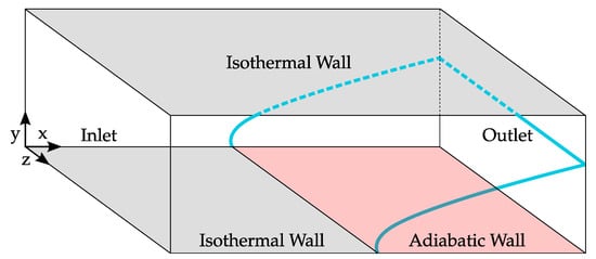
Figure 1.
Computational domain and stable flame shape for reactive LES.
The approach for obtaining flashback limits is similar to the atmospheric calculations in Reference [15]. A constant velocity is assumed in the channel at the beginning of the calculations. The species mass fractions of hydrogen, oxygen and nitrogen are set to an equivalence ratio at which no flashback is expected. The flame front is initialized by setting the temperature and species mass fractions in a rectangular box with a height of 1 to the burnt gas values. As soon as the velocity fluctuations prescribed at the inlet reach the flame front, the flame front is wrinkled and stabilizes at the leading edge of the adiabatic wall. When the flame wrinkling is fully developed, the equivalence ratio at the inlet is increased by a small step of 0.02 to 0.05. This is repeated until the flame front propagates upstream along the isothermal wall without being completely washed out. This equivalence ratio is defined as the flashback equivalence ratio .
2.3. Les Regimes for Hydrogen Combustion
The requirement for the applicability of the ILES approach is that the SGS flame either has a laminar structure, or that the reaction and mixing processes are not influenced by SGS fluctuations. The LES combustion regimes developed by Pitsch and Duchamp de Lageneste [32] can be used to point out the laminar character of the SGS flame structure in the presented simulations. In the derivation of the original LES combustion regime diagram, Pitsch and Duchamp de Lageneste assume that the diffusivity D of the gas mixture equals the kinematic viscosity . This assumption is however invalid for hydrogen combustion. In the following, the LES combustion regimes are therefore analyzed for the general case, where .
The combustion regimes are defined by the Karlovitz number and the ratio of the LES filter width to the laminar flame length scale [40], where is the laminar flame speed. The Karlovitz number is defined as the ratio of the flame time scale to the time scale of the Kolmogorov eddies. The Kolmogorov length scale can be approximated by the kinematic viscosity and the dissipation rate . Here, is the SGS turbulent kinetic energy and is a model constant. This results in the diffusivity and viscosity dependent Karlovitz number calculated from LES quantities,
The wrinkled flamelet regime and the corrugated flamelet regime are separated by the Gibson length scale. The Gibson length scale is defined by the equality of the laminar flame speed and the SGS velocity fluctuation . In the wrinkled flamelet regime, the SGS velocity fluctuation is smaller or equal to the laminar flame speed. According to Peters [40], fluctuations with a velocity smaller than the laminar flame speed do not wrinkle the flame front. The SGS flame therefore has a laminar character in the wrinkled flamelet regime while it has a non-laminar character in the corrugated flamelet regime. With the assumption that , the condition for the Gibson length scale leads to a mixture independent relation between the Karlovitz number and . For hydrogen however, and the condition for the Gibson length scale lead to
when assuming . This takes the viscosity and diffusivity of the gas mixture into account when evaluating the SGS combustion regime. This results in the different lines between the wrinkled flamelet and corrugated flamelet regime in Figure 2 and Figure 3.

Figure 2.
LES combustion regimes for .
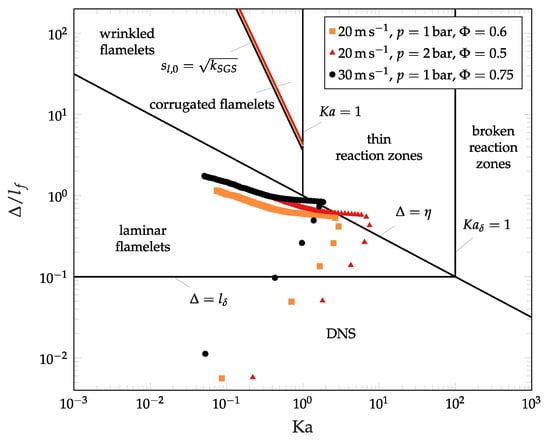
Figure 3.
LES combustion regimes for and .
Figure 2 and Figure 3 show the SGS combustion regimes at different pressure levels for the highest corresponding equivalence ratios investigated in the current work. Each data point represents one cell along the y-axis of the unrefined mesh. The velocity fluctuations are obtained from the inert calculations and the laminar flame speed is calculated from the correlation developed by Böck [41] for atmospheric flames. The influence of pressure on the laminar flame speed is taken into account by the proportionality . The pressure exponent m is obtained from the results of Bradley et al. [42]. Following Bechtold and Matalon [43], the Lewis number of gas mixtures can be obtained from the species diffusivities and a mixture and flame temperature dependent weight function.
For this calculation, the species diffusivities and and species thermal diffusivities are assumed to be mixture independent. The Zeldovich number
is calculated from the adiabatic flame temperature , the unburnt gas temperature the constant activation energy kcal mol and the universal gas constant R. With the resulting Lewis numbers and the actual mixture thermal diffusivities obtained from Cantera, the mixture diffusivities D can be computed using the Lewis number definition . The input and resulting parameters for the diffusivity calculation for all cases are listed in Table A1 in Appendix A.
It is evident from Figure 2 that all cases at lie within the laminar flamelet and the DNS regimes. In the laminar flamelet regime the filter width is smaller than the Kolmogorov length scale . The SGS flow is therefore approximately laminar and no SGS turbulence fluctuations will have an influence on the combustion process [32]. At and bar, all cells also lie within the laminar flamelet and DNS regimes. At and bar as well as at and bar, some cells lie within the thin reaction zones regime. In this regime, the SGS turbulent eddies are small enough to penetrate the flame preheat zone and affect the mixing processes in the preheat zone [32]. The cells in the thin reaction zone regime should therefore not be modeled with the ILES combustion model. This has to be taken into account when analyzing the results of the two cases. Especially for and , the majority of the cells however lie within the laminar flamelet and DNS regimes and show a laminar SGS flame structure. In order to also investigate the pressure influence for different bulk velocities, the case at and the case at are included here nevertheless. For all other cases the ILES approach is valid and the results are expected to deliver accurate results.
3. Results
The presented approach leads to flashback limits at different pressure levels with the unaltered inert base flow. In the following, the pressure influence on the flashback limits is investigated. This is followed by an analysis of the macroscopic flame structure and the flame resolution resulting from the macroscopic flame structure. Finally, the influence of pressure on the combustion and flow separation characteristics is investigated on the basis of average pressure and velocity fields and on the basis of local flame quenching and boundary layer separation.
3.1. Pressure Influence on Confined Flashback Limits
At atmospheric pressure, confined boundary layer flashback is modeled at bulk velocitites of , and . It was shown by Endres and Sattelmayer [15] that one cell split is sufficient to resolve the flame front at and . Applying two cell splits by the adaptive mesh refinement algorithm at and is furthermore prohibitive due to the associated computational costs. The adaptive mesh refinement is therefore set to a maximum of one cell split for the atmospheric simulations. With this refinement strategy, the flame is stable up to equivalence ratios of , and for bulk velocities of , and , respectively. Although flame tongues already form and propagate at these equivalence ratios, they are generally flushed out by high speed flow structures after a few millimeters of propagation. When further increasing the equivalence ratios to , and for bulk velocities of , and , flame propagation can no longer be prevented by the approaching flow and the flame is not fully flushed out of the isothermal channel section. It is noted that the flashback limit for and atmospheric pressure has increased from to compared to the results presented in Reference [15]. This is due to the changed definition of the flashback limit. Flame propagation was previously declared flashback if the flame was capable of propagating for more than 5 [15]. For and it is however observed that the flame may still be flushed out after a propagation of more than 5 . Flame propagation is therefore now only declared flashback if the flame is not fully flushed out of the isothermal channel section.
In Figure 4, the numerically obtained stable equivalence ratios and the equivalence ratios at flashback are compared with experimental flashback limits obtained by Eichler et al. [16] with a similar channel configuration. In the experiments, flashback was first observed approximately at , and . It is evident that despite a slight underestimation of the flashback tendency for bulk velocities of and , the numerical simulations are capable of reproducing the experimental flashback limits with reasonable accuracy. The simulations are therefore capable of representing the flashback process not only qualitatively but also quantitatively. This is in accordance with the findings in Reference [15], where no low Mach number approximation was applied.
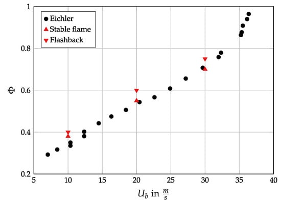
Figure 4.
Atmospheric flashback limits obtained from the reactive LES compared to experimental flashback limits of Eichler et al. [16].
In addition to the atmospheric simulations, flashback simulations are performed at a subatmospheric pressure of and at slightly elevated pressures of and . At , bulk velocities of and are numerically investigated. As the flame thickness is expected to be larger at lower pressure levels, no additional mesh refinement is necessary compared to the atmospheric simulations. Only one cell split is thus applied to the base mesh by the adaptive mesh refinement algorithm. The flame thickness is however reduced at higher pressure levels. Two cell splits are therefore applied at and a bulk velocity of . As already mentioned for the atmospheric simulations, two cell splits can not be applied to simulations with due to limited computational resources. A maximum of only one cell split is therefore applied at and . As one cell split is not expected to be sufficient for and , the investigation of the highest pressure level is limited to . Here, the initial inert mesh is refined in x-direction by increasing the cell count in x-direction by a factor of . The adaptive mesh refinement additionally refines the mesh by applying a maximum of two cell splits.
The flashback limits at different pressure levels resulting from this refinement strategy are depicted in Figure 5. Here, the flashback limit is defined as the first equivalence ratio, where the flame is not flushed out of the isothermal section of the channel. The error bars illustrate the fact that flashback might already occur at any equivalence ratio between the last stable simulation and the first simulation in which flashback occurs. For and , no flashback was observed up . The laminar flame speed obtained from Cantera simulations reaches its maximum below this equivalence ratio. Increasing the equivalence ratio beyond does therefore not increase flashback propensity and flashback is not expected to occur for and . From Figure 5 it is evident that increasing the pressure leads to lower flashback limits. Only the case at and shows an identical flashback limit compared to the lower pressure case at . At , the pressure exponent of the dependency is , , at pressures of , and compared to the flashback limit at . At , the pressure exponent is at compared to the flashback limit at . In literature, pressure exponents of unconfined flashback have been found to lie between and for H-CO-air flames and between and for H-air flames [5,6]. The numerically obtained pressure exponents for confined flames are thus similar to experimentally obtained pressure exponents for unconfined flames. In the confined simulations, there is however no unique pressure exponent for one bulk velocity. Instead, the pressure exponent for decreases with increasing pressure.
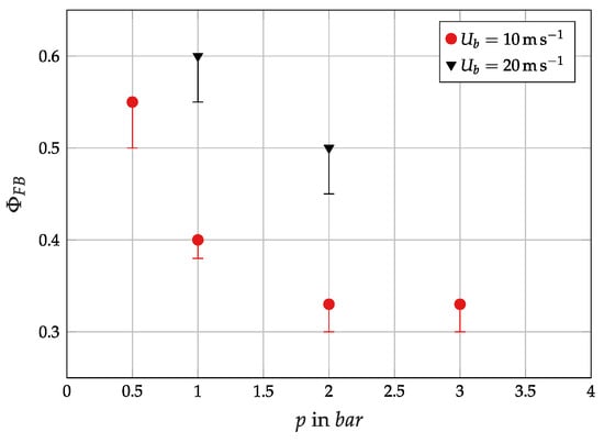
Figure 5.
Pressure influence on numerical flashback limits.
3.2. Macroscopic Flame Structure and Turbulent Flame Speed
The propagating flame fronts at all four pressure levels can be compared in Figure 6. It is evident that flame front wrinkling increases with pressure. Furthermore, the radius of the propagating flame tongue decreases with increasing pressure. This is caused by the decrease of flame thickness with higher pressure. The smaller flame thickness makes the flame more susceptible to flame wrinkling and allows for smaller flame structures. The flame thickness is defined by
where is the temperature gradient. The turbulent flame thickness is obtained by sampling the magnitude of the temperature gradient of one time step on isosurfaces of the progress variable c. The progress variable for lean mixtures is defined by the unburnt hydrogen mass fraction and the local hydrogen mass fraction :
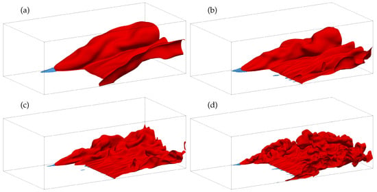
Figure 6.
Instantaneous flame fronts and separation zones during flashback at the pressure levels (a) bar, (b) 1 bar, (c) 2 bar and (d) 3 bar for . The flame front is represented by the red isosurface. The separation zone is represented by the blue isosurface.
19 isosurfaces of c between 0.05 and 0.95 from at least 27 time steps during flame flashback are considered for sampling the temperature gradient. Wall normal turbulent flame thickness profiles are obtained for each of the 19 isosurfaces by calculating the flame thickness from the streamwise, spanwise and time average of the sampled temperature gradient. A minimum average flame thickness of all flame thickness profiles is computed for each wall normal distance. This approach results in the minimum flame thickness profiles in Figure 7. It is evident that although the equivalence ratio is reduced with increasing pressure, the flame thickness significantly reduces with increasing pressure.
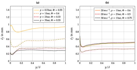
Figure 7.
Flame thickness profiles at flashback conditions for (a) and for (b) and .
The flame thickness profiles in Figure 7 can be used to obtain a minimum resolution of the simulations. The flame thickness is therefore divided by the cube root of the cell volume. This results in minimum resolutions of 3.0 cells per flame thickness for and at up to 5.5 cells per flame thickness for and at . The minimum resolution requirement of 3 cells per flame thickness [25] is thus fulfilled for all cases.
Increasing the pressure from 2 bar to 3 bar at and does not decrease the average flame thickness as strongly as at lower pressures. This is confirmed by the laminar flame thicknesses in Figure 8 obtained from freely propagating flame simulations with Cantera [38]. It is evident that at low pressures, flame thickness decreases with increasing pressure. At higher pressures, the flame thickness however increases with increasing pressure. At very high pressure levels, the flame thickness of all equivalence ratios decreases again with increasing pressure. It is therefore expected that the flame thickness is increased and the susceptibility to flame front wrinkling is decreased at low equivalence ratios and higher pressures. In addition, the laminar flame speed decreases with increasing pressure [38]. The turbulent flame speed at flashback conditions does therefore not necessarily increase with pressure.
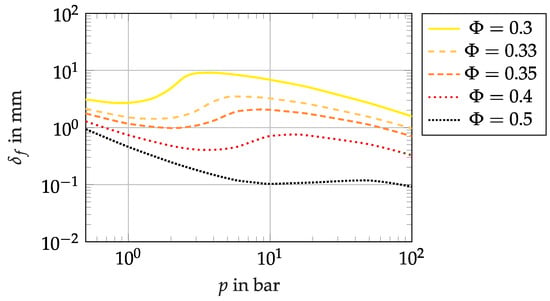
Figure 8.
Pressure dependence of the laminar flame thickness obtained from one-dimensional freely propagating flame simulations.
The turbulent flame speed in the simulations can be estimated from Figure 9, where the average stable flame shapes are shown for all operating conditions. The flame shapes are represented by isolines of the averaged progress variable, which are obtained by spatially averaging the temporal average of the hydrogen mass fraction field. The decreasing laminar flame speed at higher pressures can not be compensated by the increased flame front wrinkling due to smaller flame thicknesses. This leads to smaller average flame angles at higher pressure. The average flame shape is however only an inaccurate measure for the turbulent flame thickness. Figure 10 therefore shows the turbulent flame speed profiles of all stable cases at and . Here, the turbulent flame speed is defined as the average gas velocity component normal to the flame front [40]. This gas velocity is measured at the isoline of the average flame front. The measured gas velocity is corrected by the factor in order to account for the temperature rise to the flame temperature T at . The actual turbulent flame speeds depend on the chosen value of for the flame speed evaluation. The turbulent flame speed profiles in Figure 10 are therefore normalized by the maximum turbulent flame speed at the corresponding bulk velocity. The turbulent flame speed profiles demonstrate that the maximum turbulent flame speed at conditions close to flashback varies strongly with pressure. The maximum turbulent flame speed at and is only 73% of the maximum turbulent flame speed at and . From Equation (4), this difference in turbulent flame speed would result in a deviation of 40% in flashback channel centerline velocity. This shows that the average flame shape, the turbulent flame speed and Equation (4) are poor indicators for the susceptibility of boundary layer flashback.
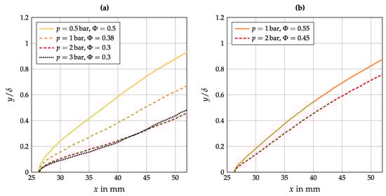
Figure 9.
Comparison of average stable flame shapes at different pressure levels evaluated at . (a) for and (b) for .
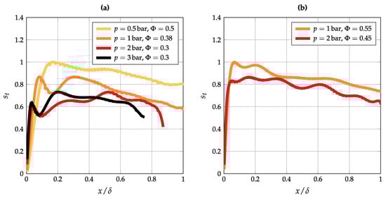
Figure 10.
Comparison of turbulent flame speeds at different pressure levels for (a) and for (b) .
3.3. Average Pressure and Velocity Fields
Eichler et al. [16] showed that confined flames induce a pressure rise ahead of the flame which leads to flow deflection away from the wall. This can also be observed in Figure 11a, where the streamlines of the time and spanwise averaged velocity field are depicted together with the average flame shape and pressure field for the stable case at and . Ahead of the flame the streamlines are deflected away from the wall. The turbulent flame brush redirects the streamlines back towards the wall. The flow redirection is caused by the fact that the tangential gas velocity is not changed by the flame front, while the velocity component normal to the flame front increases due to the density decrease across the flame. Ahead of the flame the flow is deflected away from the wall and the axial gas velocity decreases. The two-dimensional flow pattern is linked to a two-dimensional pressure field with a pressure maximum just ahead of the leading flame tip. This confirms the two-dimensional nature of the velocity field and of the pressure rise ahead of the flame observed by Eichler [11].
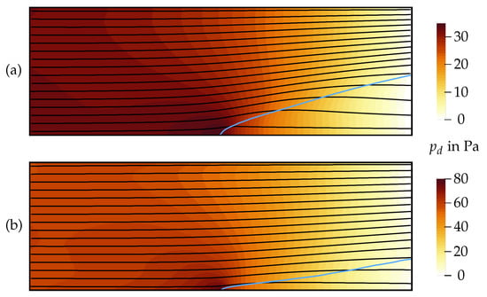
Figure 11.
Average streamlines, average flame shape and average pressure field of the stable cases at at (a) bar and at (b) bar. The average flame shape is represented by the blue isoline.
The flashback equivalence ratio decreases with increasing pressure. The expansion ratio of unburnt gas density to burnt gas density therefore also decreases with increasing pressure. This leads to weaker flow deflection at higher pressures, which can be seen when comparing the streamlines in Figure 11b for the stable case at with the streamlines in Figure 11a at . The different streamline patterns in Figure 11 show that average boundary layer separation is not an indicator for flame flashback. The boundary layer at shows stronger flow deflection and is much closer to average boundary layer separation than the boundary layer at . At elevated pressures, flashback thus occurs at reduced turbulent flame speeds, reduced expansion ratios and at reduced average flow deflection ahead of the flame. These average quantities alone can therefore not describe the flashback propensity of a flame. Instead, local processes at the flame tip, such as flame quenching and local flow separation have to be taken into account.
3.4. Quenching Distance and Local Flow Separation
In addition to the average quantities previously presented, the local quantities at the propagating flame front also show significant differences depending on the operating conditions. By tracking the flame front during flashback, the separation zone size and quenching distance during flashback are obtained. Figure 12 exemplarily shows the hydrogen reaction rate and flow separation zone on a cutting plane through the foremost flame tip during flashback at and . From this cutting plane, a wall-normal profile of the maximum hydrogen reaction rate can be obtained. The quenching distance is then defined as the wall distance of the first local maximum of this maximum hydrogen reaction rate profile. The separation zone size is the wall-normal size of the region, where the streamwise velocity .
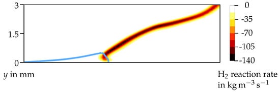
Figure 12.
Hydrogen reaction rate and flame separation during flashback. Blue line represents the isosurface.
Endres and Sattelmayer [15] showed that upstream flame propagation takes place when the separation zone size is significantly larger than the average quenching distance. This is also evident for and in Figure 13, where the x position of the foremost flame tip is compared to the separation zone size and the quenching distance during flashback. This is however not necessarily always the case. During flashback at and , upstream flame propagation also occurs in time periods where the separation zone size is considerably smaller than the quenching distance. This implies that the flame speed for this operating condition is high enough for the flame to propagate upstream at wall distances above the separation zone and not only in the backflow region of the separation zone.
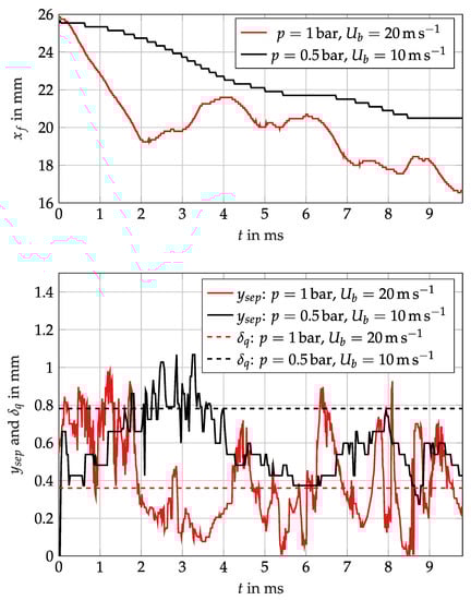
Figure 13.
Flame front position, separation zone size and quenching distance during flame flashback. Flame front position is given by the foremost cell with .
The average quenching distances and separation zone sizes during upstream propagation of all cases under investigation are listed in Table 2. The quenching distance decreases with increasing pressure. This is in accordance with the trend of the flame thickness, which also decreases with pressure. Dividing the quenching distance by the average flame thickness at the quenching wall distance from the profiles in Figure 7 results in the quenching Peclet numbers in Table 2. For head-on quenching of laminar hydrogen-oxygen and hydrogen-air flames, Dabireau et al. [44] and Gruber et al. [45] found quenching Peclet numbers of and . Except for and , where a few cells lie in the thin reaction zones regime, the current quenching Peclet numbers are of the same order of magnitude as the Peclet numbers from literature. The difference in quenching Peclet numbers are likely to arise due to the difference in quenching configuration. The Peclet numbers given here are for turbulent sidewall quenching while the cited literature values are for laminar head-on quenching.
Table 2.
Quenching and separation parameters at flashback conditions.
The average separation zone size also decreases with increasing pressure. With increasing pressure, the flame thickness and the flame tip radius decrease while the fresh gas density increases with increasing pressure. This leads to weaker flow deflection ahead of the flame, as already seen from the average streamlines in Figure 11. From Table 2 it is however evident that the ratio of separation zone size to quenching distance is not constant. For for example, it increases from 0.84 at to 2.23 at . The decrease of quenching thickness with pressure is thus stronger than the decrease of separation zone size. There is hence no unique ratio between separation zone size and quenching distance which could be used as a criterion for the onset of flame flashback.
From to , the ratio of separation zone size to quenching distance is reduced from 2.23 to 2.16. This indicates that here, the separation zone size decreases more strongly than the quenching distance. In addition to the turbulent flame speed, this is another reason why the simulation at and does not show a higher flashback equivalence ratio than at . It was shown in Section 3.2 that the laminar flame thickness increases with pressure at very lean gas mixtures and higher pressures than investigated in the present study. It is possible that the quenching distance and the separation zone size show a similar trend and increase with increasing pressure. Depending on the ratio of separation zone size to quenching distance, this may increase or decrease the flashback propensity of the confined flames at higher pressures.
3.5. Implications for Analytical Flashback Prediction
The comparison of the pressure rise estimated by the analytical model of Hoferichter et al. [9] with the pressure rise obtained from LES shows that the analytical model does not accurately predict the quantitative values of the pressure rise. According to the analytical model the pressure rise for the stable atmospheric case at and is , while in the simulations only are observed. This pressure rise is similar to the pressure rise observed with the compressible solver from Reference [15]. The low Mach number assumption thus does not have a strong effect on the average pressure rise ahead of the flame front. At and and at and the pressure rise ahead of the flame is and in the simulations. The analytical model however predicts a pressure rise of and for the same operating conditions. The pressure rise ahead of the flames of all cases is thus overestimated by the one-dimensional pressure calculation of the analytical model. At the same time, the Stratford separation criterion underestimates the separation propensity at BLF. The Stratford criterion is based on the boundary layer theory. The application of the boundary layer theory requires a uniform wall-normal pressure. Figure 14 shows the average wall-normal pressure profile just upstream of the stable atmospheric flame at . It is evident that the pressure is not constant over the channel height. Such a non-uniform pressure profile does not only cause flow deceleration but also flow deflection. This increases the tendency for boundary layer separation. The boundary layer theory and the Stratford criterion cannot be applied in this case.
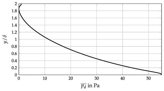
Figure 14.
Wall-normal average dynamic pressure profile ahead of the stable flame front at atmospheric pressure and .
4. Conclusions
The influence of pressure on the combustion and flow characteristics was investigated by comparing LES results of confined BLF at different pressure levels and bulk velocities. At elevated pressure the flame thickness decreases and the flame is corrugated more strongly by turbulence and thermal-diffusive instabilities. The turbulent flame speed and the flame angle at conditions close to flashback however decreased with increasing pressure. The average flow deflection ahead of the flame also decreased with increasing pressure. Lower turbulent flame speeds and weaker flow deflection ahead of the flame at higher pressure levels would imply a reduced flashback propensity at higher pressure levels. It was however shown that the flashback propensity increased with increasing pressure. The turbulent flame speed, the average flame shape and flow deflection alone are thus poor indicators for the onset of BLF.
Instead, additional quantities such as the quenching distance and the local separation zone size have to be accounted for. The quenching thickness decreases with increasing pressure. At the same time, the local separation zone size ahead of the propagating flame tip decreases with increasing pressure. The reduced flame thickness and quenching distance lead to a smaller flame tip diameter, which reduces the deflection of the approaching flow by the flame. Although these two local effects are counteracting, they do not cancel out and their influence on the flashback limits cannot be neglected. Confined BLF is instead a complex process, which is influenced by the local flame speed, the flame thickness, the quenching distance and the separation tendency of the approaching flow. The low separation zone sizes and high quenching distances at low pressure increase the flashback resistance of the flame, thus allowing for higher stable equivalence ratios. As the flame speed increases with increasing equivalence ratio at low pressures, the susceptibility of the flame to flashback increases. Usually flame propagation occurs inside the recirculating flow of the separation zone. The high flame speeds at low pressures however also allows for flame propagation in regions without recirculating flow.
Finally it was noted that the underlying assumptions of the boundary layer theory and of one-dimensional pressure approximations are not satisfied in confined BLF. The application of one-dimensional pressure approximations leads to an overestimation of the pressure rise ahead of the flame. The application of the boundary layer theory leads to an underestimation of the separation probability. These two errors are counteracting and might possibly compensate each other. Due to this inconsistency, the analytical flashback prediction model [9] should however rather be regarded as a correlation on the experimental flashback data, which is capable of accurately accounting for flashback influences such as preheat temperature or fuel composition.
Author Contributions
Conceptualization: A.E. and T.S.; methodology, software, validation, formal analysis, investigation, writing—original draft preparation, visualization: A.E.; writing—review and editing, supervision: T.S.
Funding
This research was funded by the German research foundation DFG, project No. SA 781/19-1.
Acknowledgments
The authors gratefully acknowledge the compute and data resources provided by the Leibniz Supercomputing Centre (www.lrz.de).
Conflicts of Interest
The authors declare no conflict of interest. The funders had no role in the design of the study; in the collection, analyses, or interpretation of data; in the writing of the manuscript, or in the decision to publish the results.
Abbreviations
The following abbreviations are used in this manuscript:
| BLF | Boundary Layer Flashback |
| LES | Large Eddy Simulation |
| ILES | Implicit LEL |
| ODE | Ordinary Differential Equations |
| SGS | Subgrid Scale |
Appendix A
Table A1.
Parameters for the mixture diffusivity calculation.
Table A1.
Parameters for the mixture diffusivity calculation.
| p | m | D | ||||||
|---|---|---|---|---|---|---|---|---|
| in bar | in K | in m s | in m s | in m s | in m s | |||
| 0.5 | 0.55 | 1741.4 | 0.76 | −0.26 | 7.275 | 3.722 | 0.458 | 1.587 |
| 1 | 0.4 | 1422.3 | 0.35 | −0.35 | 3.248 | 1.754 | 0.394 | 8.246 |
| 1 | 0.6 | 1838.6 | 0.92 | −0.24 | 3.698 | 1.864 | 0.484 | 7.640 |
| 1 | 0.75 | 2096.8 | 1.40 | −0.18 | 4.003 | 1.944 | 0.572 | 7.000 |
| 2 | 0.33 | 1257.2 | 0.20 | −0.40 | 1.559 | 8.689 | 0.370 | 4.212 |
| 2 | 0.5 | 1640.7 | 0.61 | −0.29 | 1.763 | 9.166 | 0.435 | 4.053 |
| 3 | 0.33 | 1257.2 | 0.20 | −0.40 | 1.039 | 5.793 | 0.370 | 2.808 |
References
- Bolland, O.; Undrum, H. A novel methodology for comparing CO2 capture options for natural gas-fired combined cycle plants. Adv. Environ. Res. 2003, 7, 901–911. [Google Scholar] [CrossRef]
- Voldsund, M.; Jordal, K.; Anantharaman, R. Hydrogen production with CO2 capture. Int. J. Hydrogen Energy 2016, 41, 4969–4992. [Google Scholar] [CrossRef]
- Schorr, M.M.; Chalfin, J. Gas Turbine NOx Emissions Approaching Zero — Is It Worth the Price? General Electric Power Generation, Report No. GER 4172; General Electric Power: Schenectady, NY, USA, 1999. [Google Scholar]
- Gruber, A.; Chen, J.H.; Valiev, D.; Law, C.K. Direct numerical simulation of premixed flame boundary layer flashback in turbulent channel flow. J. Fluid Mech. 2012, 709, 516–542. [Google Scholar] [CrossRef]
- Daniele, S.; Jansohn, P.; Boulouchos, K. Flashback Propensity of Syngas Flames at High Pressure: Diagnostic and Control. In Combustion, Fuels and Emissions, Parts A and B; ASME: Glasgow, UK, 2010; Volume 2, pp. 1169–1175. [Google Scholar] [CrossRef]
- Kalantari, A.; Sullivan-Lewis, E.; McDonell, V. Flashback Propensity of Turbulent Hydrogen–Air Jet Flames at Gas Turbine Premixer Conditions. J. Eng. Gas Turbines Power 2016, 138, 061506. [Google Scholar] [CrossRef]
- Eichler, C.; Sattelmayer, T. Experiments on flame flashback in a quasi-2D turbulent wall boundary layer for premixed methane-hydrogen-air mixtures. J. Eng. Gas Turbines Power 2011, 133, 011503. [Google Scholar] [CrossRef]
- Hoferichter, V.; Sattelmayer, T. Boundary Layer Flashback in Premixed Hydrogen–Air Flames with Acoustic Excitation. J. Eng. Gas Turbines Power 2018, 140, 051502. [Google Scholar] [CrossRef]
- Hoferichter, V.; Hirsch, C.; Sattelmayer, T. Prediction of Confined Flame Flashback Limits Using Boundary Layer Separation Theory. J. Eng. Gas Turbines Power 2017, 139, 021505. [Google Scholar] [CrossRef]
- Stratford, B.S. The prediction of separation of the turbulent boundary layer. J. Fluid Mech. 1959, 5, 1–16. [Google Scholar] [CrossRef]
- Eichler, C.T. Flame Flashback in Wall Boundary Layers of Premixed Combustion Systems; Verlag Dr. Hut: München, Germany, 2011. [Google Scholar]
- Gruber, A.; Richardson, E.S.; Aditya, K.; Chen, J.H. Direct numerical simulations of premixed and stratified flame propagation in turbulent channel flow. Phys. Rev. Fluids 2018, 3. [Google Scholar] [CrossRef]
- Clemens, N. Large Eddy Simulation Modeling of Flashback and Flame Stabilization in Hydrogen-Rich Gas Turbines Using a Hierarchical Validation Approach; University of Texas: Austin, TX, USA, 2015. [Google Scholar] [CrossRef]
- Lietz, C.; Hassanaly, M.; Raman, V.; Kolla, H.; Chen, J.; Gruber, A. LES of Premixed Flame Flashback in a Turbulent Channel. In Proceedings of the 52nd Aerospace Sciences Meeting, National Harbor, MD, USA, 13–17 January 2014; American Institute of Aeronautics and Astronautics: Reston, VA, USA, 2014. [Google Scholar] [CrossRef]
- Endres, A.; Sattelmayer, T. Large Eddy simulation of confined turbulent boundary layer flashback of premixed hydrogen-air flames. Int. J. Heat Fluid Flow 2018, 72, 151–160. [Google Scholar] [CrossRef]
- Eichler, C.; Baumgartner, G.; Sattelmayer, T. Experimental Investigation of Turbulent Boundary Layer Flashback Limits for Premixed Hydrogen-Air Flames Confined in Ducts. J. Eng. Gas Turb. Power 2012, 134, 011502. [Google Scholar] [CrossRef]
- Weller, H.G.; Tabor, G.; Jasak, H.; Fureby, C. A tensorial approach to computational continuum mechanics using object-oriented techniques. Comput. Phys. 1998, 12, 620. [Google Scholar] [CrossRef]
- Jasak, H. Error Analysis and Estimation for Finite Volume Method with Applications to Fluid Flow. Ph.D. Thesis, University of London, London, UK, June 1996. [Google Scholar]
- Nozaki, F. Smagorinsky SGS Model in OpenFOAM. Available online: https://caefn.com/openfoam/smagorinsky-sgs-model (accessed on 1 June 2019).
- Smagorinsky, J. General circulation experiments with the primitive equations: I. The basic experiment. Mon. Weather Rev. 1963, 91, 99–164. [Google Scholar] [CrossRef]
- Lilly, D.K. The representation of small scale turbulence in numerical simulation experiments. In Proceedings of the IBM Scientific Computing Symposium on Environmental Sciences, Yorktown Heights, NY, USA, 14–16 November 1966; pp. 195–210. [Google Scholar]
- van Driest, E.R. On turbulent flow near a wall. J. Aerosp. Sci. 1956, 23, 1007–1011. [Google Scholar] [CrossRef]
- Mukha, T.; Liefvendahl, M. Large-Eddy Simulation of Turbulent Channel Flow; Technical Report Number 2015-014; Uppsala University: Uppsala, Sweden, 2015. [Google Scholar]
- Pope, S.B. Turbulent Flows; Cambridge University Press: Cambridge, MA, USA, 2000. [Google Scholar]
- Duwig, C.; Nogenmyr, K.J.; Chan, C.k.; Dunn, M.J. Large Eddy Simulations of a piloted lean premix jet flame using finite-rate chemistry. Combust. Theory Model. 2011, 15, 537–568. [Google Scholar] [CrossRef]
- Hairer, E.; Wanner, G. Solving Ordinary Differential Equations II; Springer Series in Computational Mathematics; Springer: Berlin/Heidelberg, Germany, 1996; Volume 14. [Google Scholar] [CrossRef]
- Burke, M.P.; Chaos, M.; Ju, Y.; Dryer, F.L.; Klippenstein, S.J. Comprehensive H2/O2 kinetic model for high-pressure combustion. Int. J. Chem. Kinet. 2012, 44, 444–474. [Google Scholar] [CrossRef]
- Contino, F.; Jeanmart, H.; Lucchini, T.; D’Errico, G. Coupling of in situ adaptive tabulation and dynamic adaptive chemistry: An effective method for solving combustion in engine simulations. Proc. Combust. Inst. 2011, 33, 3057–3064. [Google Scholar] [CrossRef]
- Pope, S. Computationally efficient implementation of combustion chemistry using in situ adaptive tabulation. Combust. Theory Model. 1997, 1, 41–63. [Google Scholar] [CrossRef]
- Krüger, O.; Duwig, C.; Terhaar, S.; Paschereit, C.O. Ultra-Wet Operation of a Hydrogen Fueled GT Combustor: Large Eddy Simulation Employing Detailed Chemistry. In Proceedings of the Seventh International Conference on Computational Fluid Dynamics (ICCFD7), ICCFD7-3403, Big Island, HI, USA, 9–13 July 2012. [Google Scholar]
- Fureby, C. Comparison of flamelet and finite rate chemistry LES for premixed turbulent combustion. In Proceedings of the 45th AIAA Aerospace Sciences Meeting and Exhibit, Reno, Nevada, 8–11 January 2007; p. 1413. [Google Scholar]
- Pitsch, H.; Duchamp de Lageneste, L. Large-eddy simulation of premixed turbulent combustion using a level-set approach. Proc. Combust. Inst. 2002, 29, 2001–2008. [Google Scholar] [CrossRef]
- Heimerl, J.M.; Coffee, T.P. Transport Algorithms for Methane Flames. Combust. Sci. Technol. 1983, 34, 31–43. [Google Scholar] [CrossRef]
- Kee, R.J.; Rupley, F.M.; Meeks, E.; Miller, J.A. CHEMKIN-III: A FORTRAN Chemical Kinetics Package for the Analysis of Gas-Phase Chemical and Plasma Kinetics; Sandia National Laboratories Report SAND96-8216; Sandia National Laboratories: Albuquerque, NW, USA, 1996. [Google Scholar]
- Hirschfelder, J.O.; Bird, R.B.; Spotz, E.L. The Transport Properties of Gases and Gaseous Mixtures. II. Chem. Rev. 1949, 44, 205–231. [Google Scholar] [CrossRef] [PubMed]
- Welty, J.R. Fundamentals of Momentum, Heat, and Mass Transfer, 5th ed.; Wiley: Hoboken, NJ, USA, 2008. [Google Scholar]
- Kuo, K.K.; Acharya, R. Applications of Turbulent and Multiphase Combustion; Wiley: Hoboken, NJ, USA, 2012. [Google Scholar]
- Goodwin, D.G.; Moffat, H.K.; Speth, R.L. Cantera: An Object-oriented Software Toolkit for Chemical Kinetics, Thermodynamics, and Transport Processes. 2017. Available online: http://www.cantera.org/ (accessed on 1 June 2019). [CrossRef]
- Sutherland, W. LII. The viscosity of gases and molecular force. Philos. Mag. Ser. 5 1893, 36, 507–531. [Google Scholar] [CrossRef]
- Peters, N. Turbulent Combustion; Cambridge Monographs on Mechanics, Cambridge University Press: Cambridge, UK; New York, NY, USA, 2000. [Google Scholar]
- Böck, L.R. Deflagration-to-Detonation Transition and Detonation Propagation in H2-Air Mixtures with Transverse Concentration Gradients. Ph.D. Thesis, Technische Universität München, München, Germany, 2015. [Google Scholar]
- Bradley, D.; Lawes, M.; Liu, K.; Verhelst, S.; Woolley, R. Laminar burning velocities of lean hydrogen–air mixtures at pressures up to 1.0 MPa. Combust. Flame 2007, 149, 162–172. [Google Scholar] [CrossRef]
- Bechtold, J.K.; Matalon, M. The dependence of the Markstein length on stoichiometry. Combust. Flame 2001, 127, 1906–1913. [Google Scholar] [CrossRef]
- Dabireau, F.; Cuenot, B.; Vermorel, O.; Poinsot, T. Interaction of flames of H2 + O2 with inert walls. Combust. Flame 2003, 135, 123–133. [Google Scholar] [CrossRef]
- Gruber, A.; Sankaran, R.; Hawkes, E.R.; Chen, J.H. Turbulent flame–wall interaction: A direct numerical simulation study. J. Fluid Mech. 2010, 658, 5–32. [Google Scholar] [CrossRef]


© 2019 by the authors. Licensee MDPI, Basel, Switzerland. This article is an open access article distributed under the terms and conditions of the Creative Commons Attribution (CC BY) license (http://creativecommons.org/licenses/by/4.0/).