Conjugate Heat Transfer and Fluid Flow Modeling for Liquid Microjet Impingement Cooling with Alternating Feeding and Draining Channels


Abstract
:1. Introduction
2. Conjugate Heat Transfer and Fluid Flow Model
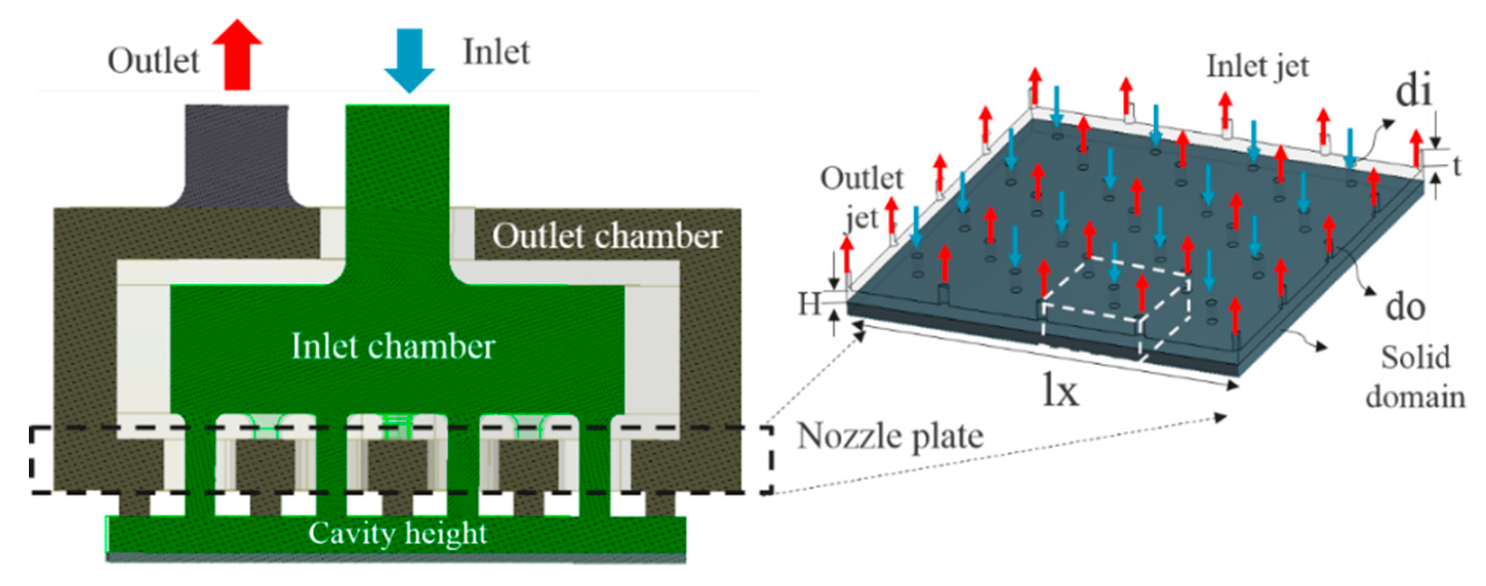
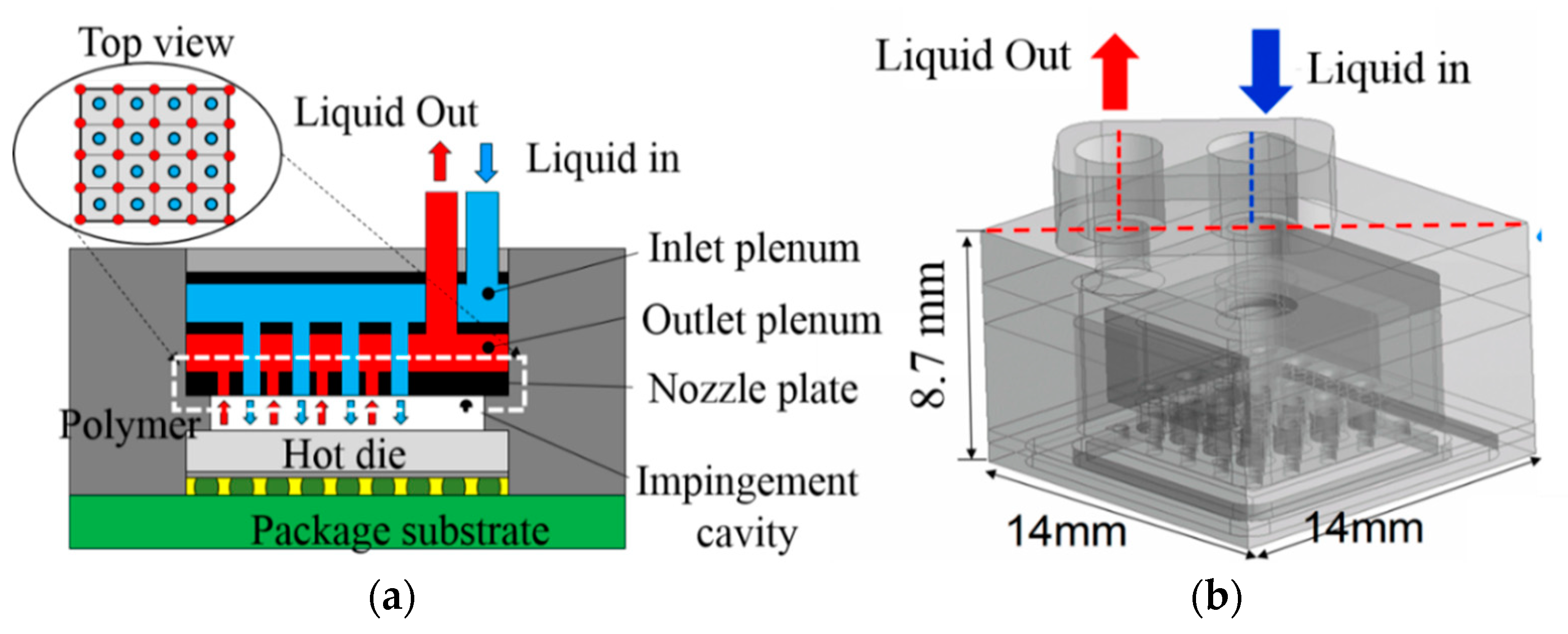
2.1. Miroject Cooling Test Case
2.2. CFD Model Introduction
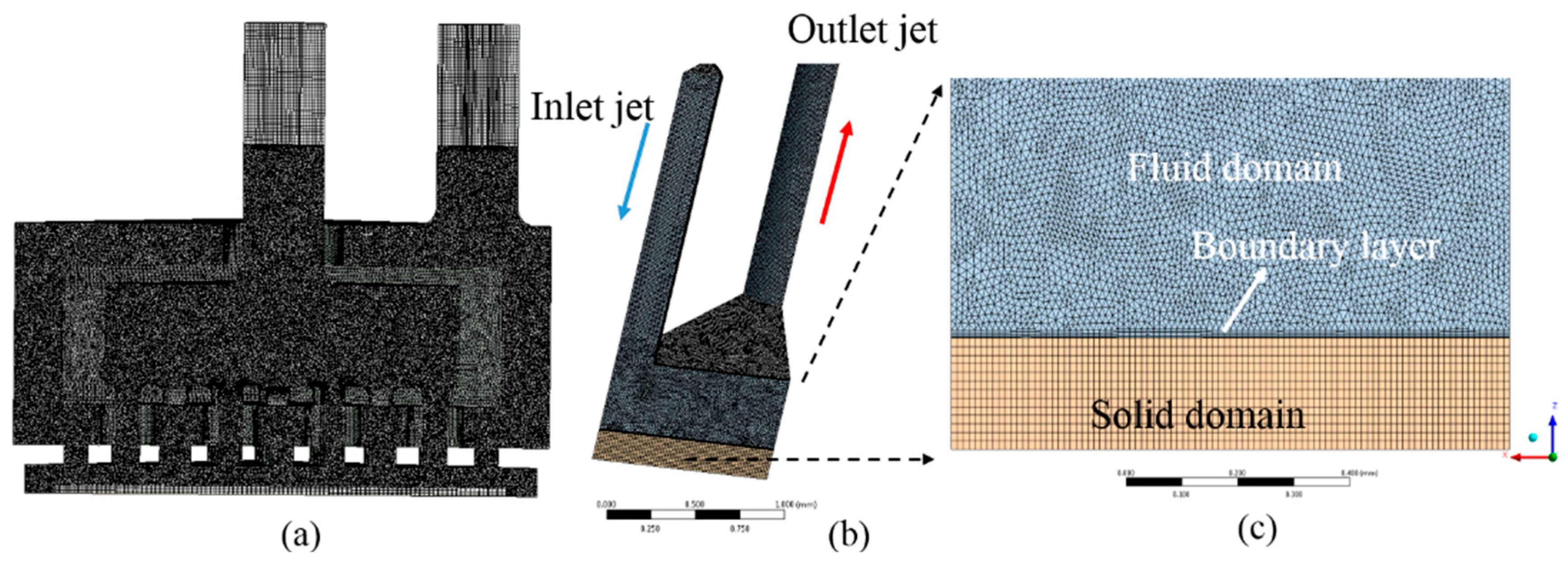
2.3. Grid Sensitivity Study
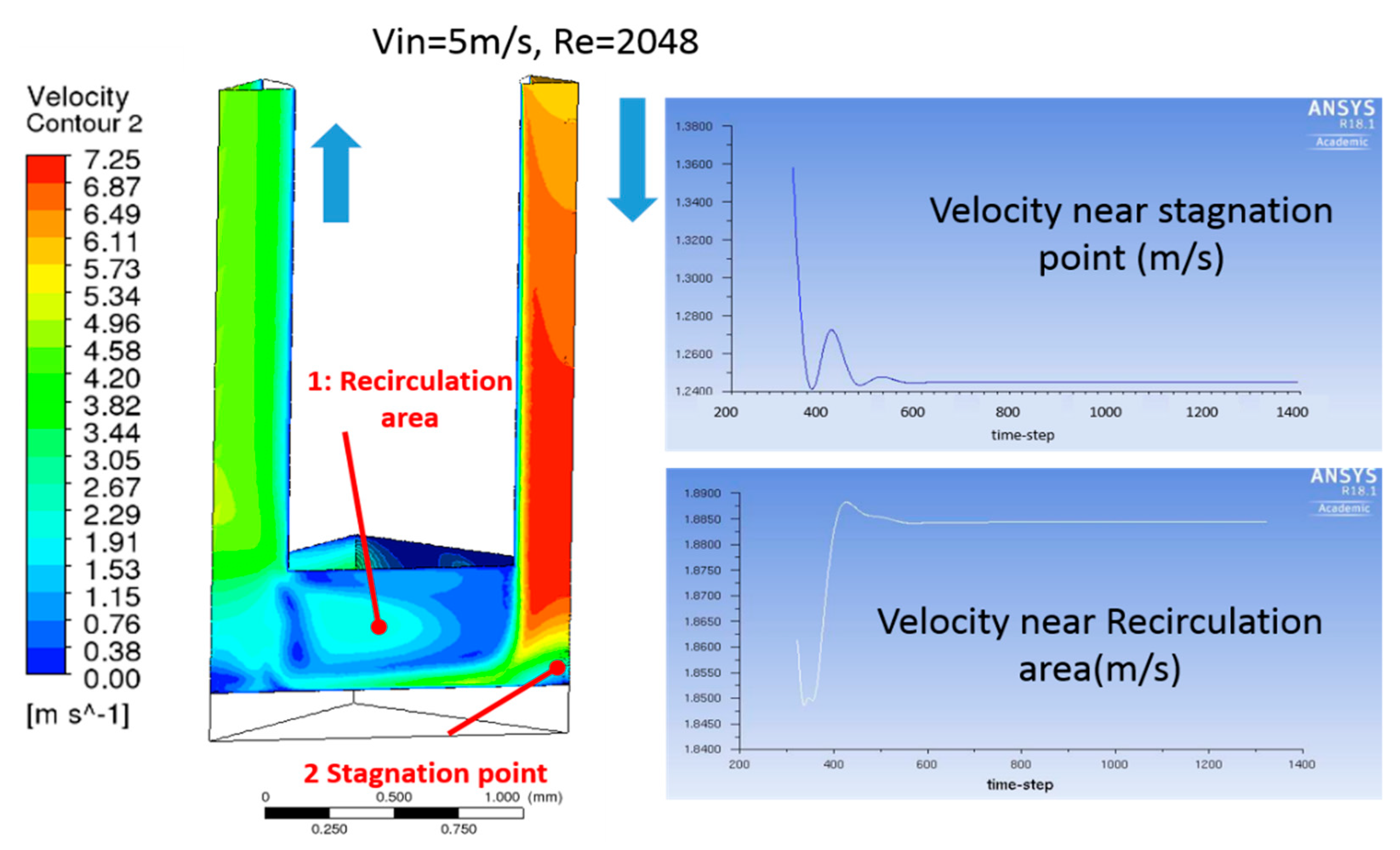
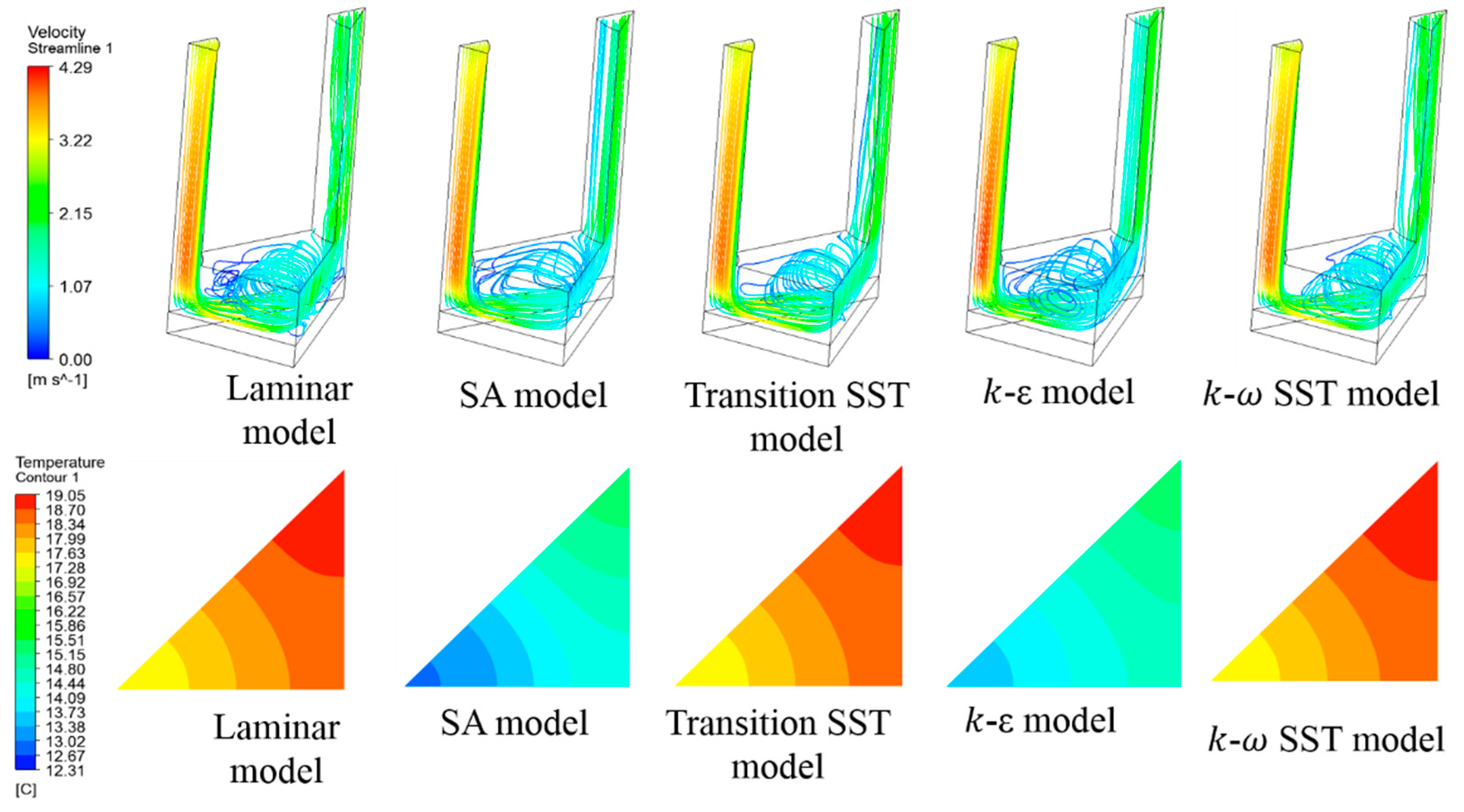
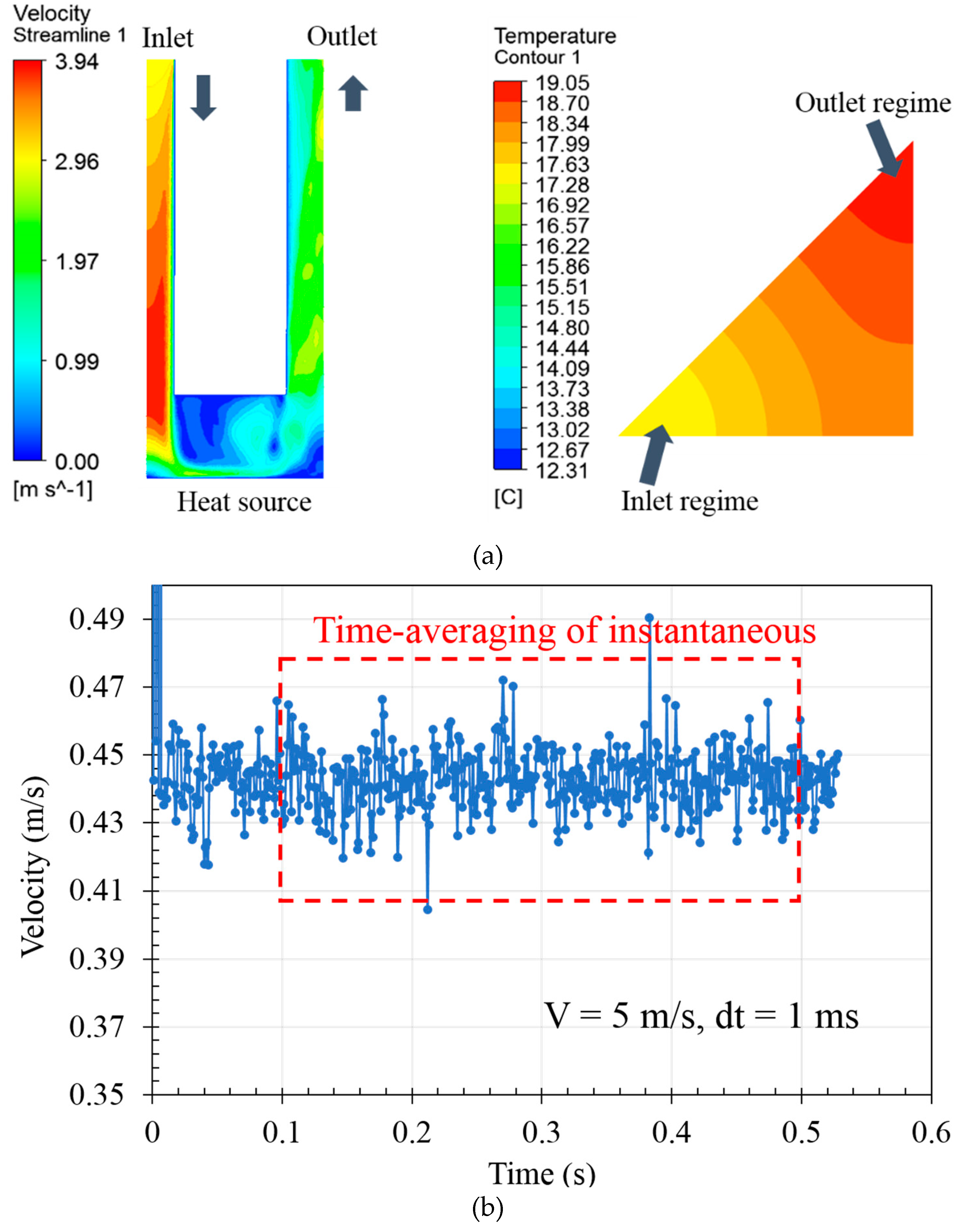
2.4. Modeling Methodology
3. Numerical Modeling Analysis
3.1. Unit Cell Modeling Analysis
3.2. Full Cooler Level Modeling Analysis
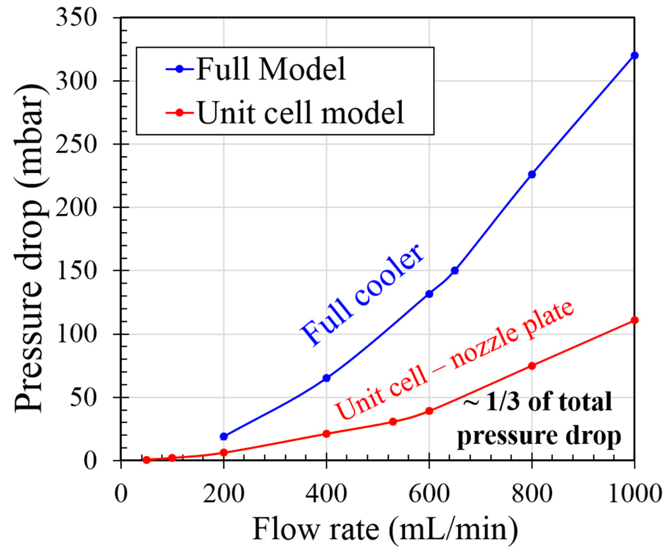
3.3. Unit Cell versus Full Level Model
4. Experimental Validation
4.1. Test Case Demonstration
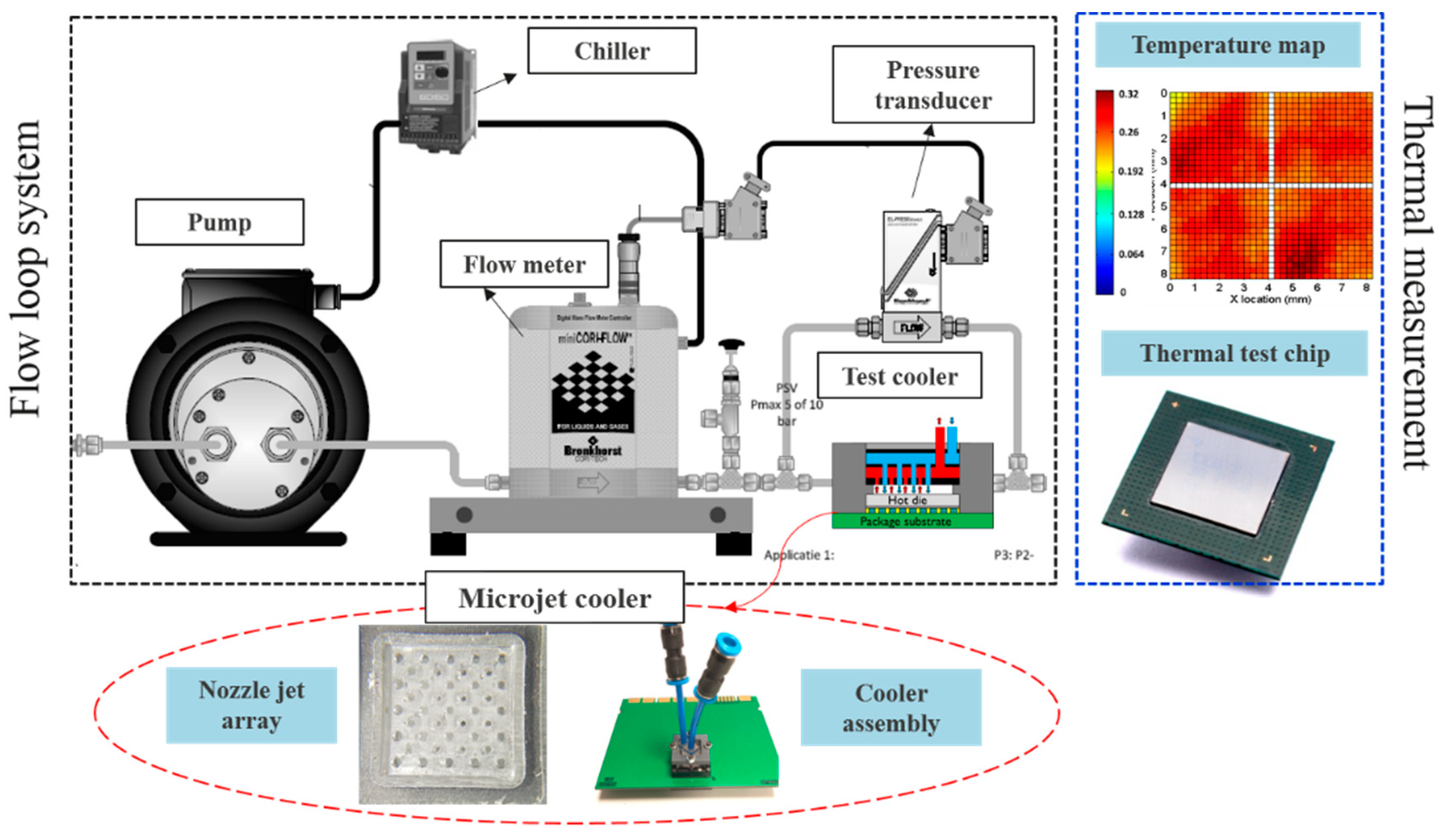
4.2. Experimental Set-Up
4.3. Results and Discussions
5. Conclusions
Author Contributions
Funding
Acknowledgments
Conflicts of Interest
References
- Jörg, J.; Taraborrelli, S.; Sarriegui, G.; De Doncker, R.W.; Kneer, R.; Rohlfs, W. Direct Single Impinging Jet Cooling of a mosfet Power Electronic Module. IEEE Trans. Power Electron. 2018, 33, 4224–4237. [Google Scholar] [CrossRef]
- Wei, T.-W.; Oprins, H.; Cherman, V.; Van der Plas, G.; De Wolf, I.; Beyne, E.; Baelmans, M. High efficiency direct liquid jet impingement cooling of high power devices using a 3D-shaped polymer cooler. In Proceedings of the 2017 IEEE International Electron Devices Meeting (IEDM), San Francisco, CA, USA, 2–6 December 2017. [Google Scholar]
- Bhunia, A.; Chen, C.L. On the scalability of liquid microjet array impingement cooling for large area systems. J. Heat Transf. 2011, 133, 064501. [Google Scholar] [CrossRef]
- Bhunia, A.; Chandrasekaran, S.; Chen, C.L. Performance improvement of a power conversion module by liquid micro-jet impingement cooling. IEEE Trans. Compon. Packag. Technol. 2007, 30, 309–316. [Google Scholar] [CrossRef]
- Robinson, A.J.; Schnitzler, E. An experimental investigation of free and submerged miniature liquid jet array impingement heat transfer. Exp. Therm. Fluid Sci. 2007, 32, 1–13. [Google Scholar] [CrossRef]
- Molana, M.H.; Banooni, S. Investigation of heat transfer processes involved liquid impingement jets: A review. Braz. J. Chem. Eng. 2013, 30, 413–435. [Google Scholar] [CrossRef]
- Han, Y.; Lau, B.L.; Zhang, H.; Zhang, X. Package-level Si-based micro-jet impingement cooling solution with multiple drainage micro-trenches. In Proceedings of the 2014 IEEE 16th Electronics Packaging Technology Conference (EPTC), Singapore, 3–5 December 2014; pp. 330–334. [Google Scholar]
- Brunschwiler, T.; Rothuizen, H.; Fabbri, M.; Kloter, U.; Michel, B.; Bezama, R.J.; Natarajan, G. Direct Liquid Jet-Impringement Cooling with Micron-Sized Nozzle Array and Distributed Return Architecture. In Proceedings of the Thermal and Thermomechanical Proceedings 10th Intersociety Conference on Phenomena in Electronics Systems, San Diego, CA, USA, 30 May–2 June 2006; pp. 193–203. [Google Scholar]
- Natarajan, G.; Bezama, R.J. Microjet cooler with distributed returns. Heat Transf. Eng. 2007, 28, 779–787. [Google Scholar] [CrossRef]
- Boldman, D.R.; Brinich, P.F. Mean Velocity, Turbulence Intensity, and Scale in a Subsonic Turbulent Jet Impinging Normal to a Large Flat Plate; NASA Lweis Center: Cleveland, OH, USA, 1977. [Google Scholar]
- Pope, S.B. Turbulent flows. Meas. Sci. Technol. 2001, 12, 11. [Google Scholar] [CrossRef]
- Zuckerman, N. Jet Impingement Heat Transfer: Physics, Correlations, and Numerical Modeling. Adv. Heat Transf. 2006, 39, 565–631. [Google Scholar]
- Viskanta, R. Heat transfer to impinging isothermal gas and flame jets. Exp. Therm. Fluid Sci. 1993, 6, 111–134. [Google Scholar] [CrossRef]
- Bernhard, W. Multiple Jet Impingement—A Review. Heat Transf. Res. 2011, 42, 101–142. [Google Scholar] [CrossRef]
- Narumanchi, S.V.J.; Hassani, V.; Bharathan, D. Modeling Single-Phase and Boiling Liquid Jet Impingement Cooling in Power Electronics; National Renewable Energy Laboratory (NREL): Golden, CO, USA, 2005. [Google Scholar]
- Womac, D.J.; Ramadhyani, S.S.; Incropera, F.P. Correlating Equations for Impingement Cooling of Small Heat Sources With Single Circular Liquid Jets. ASME J. Heat Transf. 1993, 115, 106–115. [Google Scholar] [CrossRef]
- Garimella, S.V.; Rice, R.A. Confined and submerged liquid jet impingement heat transfer. ASME J. Heat Transf. 1995, 117, 871–877. [Google Scholar] [CrossRef]
- Isman, M.K.; Pulat, E.; Etemoglu, A.B.; Can, M. Numerical Investigation of Turbulent Impinging Jet Cooling of a Constant Heat Flux Surface. Numer. Heat Transf. Part A Appl. 2008, 53, 1109–1132. [Google Scholar] [CrossRef]
- Esch, T.; Menter, F. Heat transfer predictions based on two-equation turbulence models with advanced wall treatment. Turbul. Heat Mass Transf. 2003, 4, 633–640. [Google Scholar]
- Maddox, J.F. Liquid Jet Impingement with Spent Flow Management for Power Electronics Cooling. Ph.D. Thesis, Auburn University, Auburn, AL, USA, 2015. [Google Scholar]
- Prabhakar, S.; Arun, K. Micro-Scale Nozzled Jet Heat Transfer Distributions and Flow Field Entrainment Effects Directly on Die. In Proceedings of the 18th IEEE ITHERM Conference, Las Vegas, NV, USA, 28–31 May 2019; pp. 1082–1097. [Google Scholar]
- Sung, M.K.; Mudadar, I. Effects of jet pattern on single-phase cooling performance of hybrid micro-channel/micro-circular-jet-impingement thermal management scheme. Int. J. Heat Mass Transf. 2008, 51, 4614–4627. [Google Scholar] [CrossRef]
- Polat, S.; Huang, B.; Majumdar, A.S.; Douglas, W.J.M. Numerical Flow and Heat Transfer under Impinging Jets: A Review. Annu. Rev. Heat Transf. 1989, 2, 157–197. [Google Scholar] [CrossRef]
- Behnia, M.; Parneix, S.; Dur, P. Accurate modeling of impinging jet heat transfer. In Center for Turbulence Research, Annual Research Briefs 1997; Stanford University: Stanford, CA, USA, 1997; pp. 149–164. [Google Scholar]
- Gao, S.; Voke, P.R. Large-eddy simulation of turbulent heat transport in enclosed impinging jets. Int. J. Heat Fluid Flow 1995, 16, 349–356. [Google Scholar] [CrossRef]
- Beaubert, F.; Viazzo, S. Large Eddy Simulation of a plane impinging jet. Comptes Rendus Mécanique 2002, 330, 803–810. [Google Scholar] [CrossRef]
- Hällqvist, T. Large Eddy Simulation of Impinging Jets with Heat Transfer Licentiate Thesis. Ph.D. Thesis, Royal Institute of Technology, Stockholm, Sweden, 2006. [Google Scholar]
- Olsson, M.; Fuchs, L. Large eddy simulations of a forced semiconfined circular impinging jet. Phys. Fluids 1998, 10, 476–486. [Google Scholar] [CrossRef]
- Anupam, D.; Rabijit, D.; Balaji, S. Recent Trends in Computation of Turbulent Jet Impingement Heat Transfer. Heat Transf. Eng. 2012, 33, 447–460. [Google Scholar]
- Cziesla, T.; Biswas, G.; Chattopadhyay, H.; Mitra, N.K. Large-eddy simulation of flow and heat transfer in an impinging slot jet. Int. J. Heat Fluid Flow 2001, 22, 500–508. [Google Scholar] [CrossRef]
- Draksler, M.; Končar, B.; Cizelj, L.; Ničeno, B. Large Eddy Simulation of Multiple Impinging Jets in Hexagonal Configuration—Flow Dynamics and Heat Transfer Characteristics. Int. J. Heat Mass Transf. 2017, 109, 16–27. [Google Scholar] [CrossRef]
- Acikalin, T.; Schroeder, C. Direct liquid cooling of bare die packages using a microchannel cold plate. In Proceedings of the Fourteenth Intersociety Conference on Thermal and Thermomechanical Phenomena in Electronic Systems (ITherm), Orlando, FL, USA, 27–30 May 2014; pp. 673–679. [Google Scholar]
- Wei, T.-W.; Oprins, H.; Cherman, V.; Qian, J.; De Wolf, I.; Beyne, E.; Baelmans, M. High efficiency polymer based direct multi-jet impingement cooling solution for high power devices. IEEE Trans. Power Electron. 2018, 34, 6601–6612. [Google Scholar] [CrossRef]
- Wei, T.-W.; Oprins, H.; Cherman, V.; Shoufeng, Y.; De Wolf, I.; Beyne, E.; Baelmans, M. Experimental Characterization of a Chip Level 3D Printed Microjet Liquid Impingement Cooler for High Performance Systems. IEEE Trans. Compon. Packag. Manuf. Technol. 2019. [Google Scholar] [CrossRef]
- Penumadu, P.S. Numerical investigations of heat transfer and pressure drop characteristics in multiple jet impingement system. Appl. Therm. Eng. 2017, 110, 1511–1524. [Google Scholar] [CrossRef]
- Menter, F.R.; Langtry, R.B.; Likki, S.R.; Suzen, Y.B.; Huang, P.G.; Völker, S. A correlation-based transition model using local variable—part I: Model formulation. J. Turbomach. 2006, 128, 413–422. [Google Scholar] [CrossRef]
- Mishra, A.A.; Iaccarino, G. Uncertainty estimation for reynolds-averaged navier–stokes predictions of high-speed aircraft nozzle jets. AIAA J. 2017, 55, 3999–4004. [Google Scholar] [CrossRef]
- Granados-Ortiz, F.J.; Arroyo, C.P.; Puigt, G.; Lai, C.H.; Airiau, C. On the influence of uncertainty in computational simulations of a high-speed jet flow from an aircraft exhaust. Comput. Fluids 2019, 180, 139–158. [Google Scholar] [CrossRef]
- Mishra, A.A.; Mukhopadhaya, J.; Iaccarino, G.; Alonso, J. Uncertainty Estimation Module for Turbulence Model Predictions in SU2. AIAA J. 2018, 57, 1066–1077. [Google Scholar] [CrossRef]


| Temperature | GCI12 | Asymptotic Range of Convergence |
|---|---|---|
| Stagnation Temp | 0.002 | 0.99 |
| Averaged chip Temp | 0.004 | 1.01 |
| Model | Full Model | Unit Cell Model Reynolds-Averaged Navier–Stokes (RANS) | Unit Cell Model Large Eddy Simulations (LES) |
|---|---|---|---|
| Elements | 8.5 M | 0.4 M | 3 M |
| Minimal Grid size | 80 µm | 20 µm | 1 µm |
| Computation time | 24 h | 2 h | 12 h |
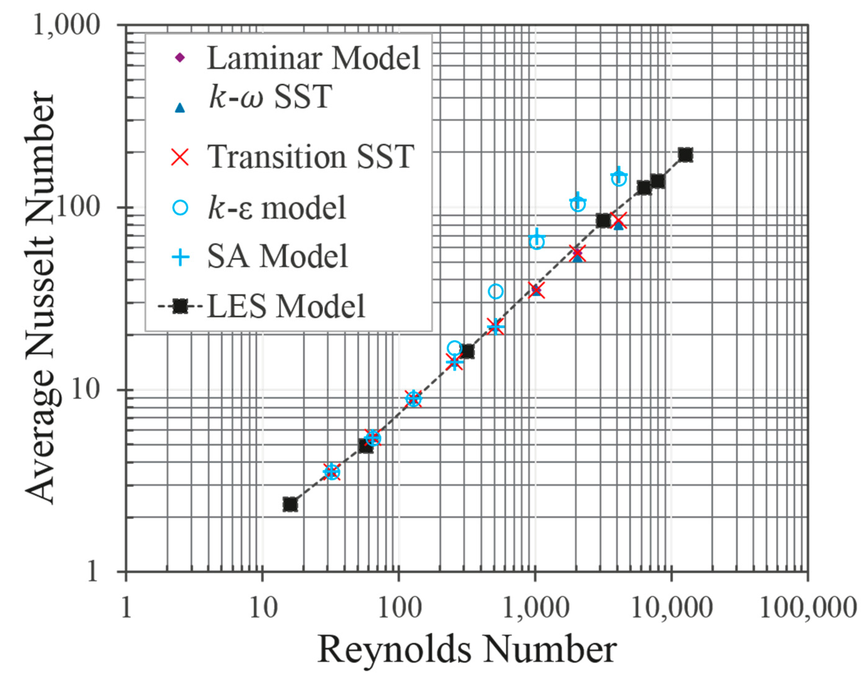
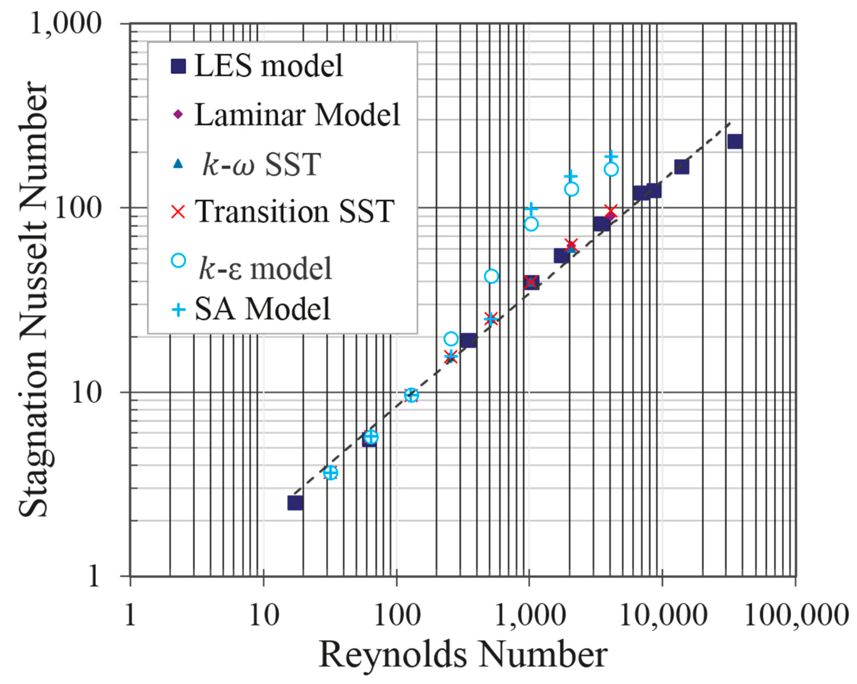
| Turbulent Model | Re | Nuavg | Nuavg Difference | Nu0 | Nu0 Difference |
|---|---|---|---|---|---|
| LES model | 1024 | 35.14 | 0 | 39.42 | 0 |
| Laminar model | 1024 | 34.92 | 0.6% | 39.42 | 0.1% |
| - SST | 1024 | 34.84 | 0.9% | 39.37 | 0.1% |
| Transition SST | 1024 | 35.05 | 0.3% | 39.53 | 0.3% |
| k-ε model | 1024 | 64.94 | 84.8% | 81.95 | 107.9% |
| SA model | 1024 | 69.27 | 97.1% | 98.28 | 149.3% |
© 2019 by the authors. Licensee MDPI, Basel, Switzerland. This article is an open access article distributed under the terms and conditions of the Creative Commons Attribution (CC BY) license (http://creativecommons.org/licenses/by/4.0/).
Share and Cite
Wei, T.; Oprins, H.; Cherman, V.; Beyne, E.; Baelmans, M. Conjugate Heat Transfer and Fluid Flow Modeling for Liquid Microjet Impingement Cooling with Alternating Feeding and Draining Channels. Fluids 2019, 4, 145. https://doi.org/10.3390/fluids4030145
Wei T, Oprins H, Cherman V, Beyne E, Baelmans M. Conjugate Heat Transfer and Fluid Flow Modeling for Liquid Microjet Impingement Cooling with Alternating Feeding and Draining Channels. Fluids. 2019; 4(3):145. https://doi.org/10.3390/fluids4030145
Chicago/Turabian StyleWei, Tiwei, Herman Oprins, Vladimir Cherman, Eric Beyne, and Martine Baelmans. 2019. "Conjugate Heat Transfer and Fluid Flow Modeling for Liquid Microjet Impingement Cooling with Alternating Feeding and Draining Channels" Fluids 4, no. 3: 145. https://doi.org/10.3390/fluids4030145
APA StyleWei, T., Oprins, H., Cherman, V., Beyne, E., & Baelmans, M. (2019). Conjugate Heat Transfer and Fluid Flow Modeling for Liquid Microjet Impingement Cooling with Alternating Feeding and Draining Channels. Fluids, 4(3), 145. https://doi.org/10.3390/fluids4030145