Stability Analysis on Nonequilibrium Supersonic Boundary Layer Flow with Velocity-Slip Boundary Conditions

Abstract

This paper presents our recent work on investigating velocity slip boundary conditions’ effects on supersonic flat plate boundary layer flow stability. The velocity-slip boundary conditions are adopted and the flow properties are obtained by solving boundary layer equations. Stability analysis of two such boundary layer flows is performed by using the Linear stability theory. A global method is first utilized to obtain approximate discrete mode values. A local method is then utilized to refine these mode values. All the modes in these two scenarios have been tracked upstream-wisely towards the leading edge and also downstream-wisely. The mode values for the no-slip flows agree well with the corresponding past results in the literature. For flows with slip boundary conditions, a stable and an unstable modes are detected. Mode tracking work is performed and the results illustrate that the resonance phenomenon between the stable and unstable modes is delayed with slip boundary conditions. The enforcement of the slip boundary conditions also shortens the unstable mode region. As to the conventional second mode, flows with slip boundary conditions can be more stable streamwisely when compared with the results for corresponding nonslip flows.

1. Introduction

Boundary layer (B.L.) flow transitions are important in many engineering fields. One example is the prediction of drag and heat transfer rates in the aircraft preliminary design stages [1]. The thickness of a thermal protection layer over a hypersonic re-entry spacecraft is estimated with the surface heat transfer rate which can be several times larger in the turbulent B.L. than a laminar one [2,3,4]. Slip boundary condition (B.C.) effects on flow stability have received much attention with new developments and applications in: (1) Micro-Electro-Mechanical System (MEMS) [5,6]; (2) slip flows in porous medium [7,8]; and (3) high speed flights with low air density [9,10]. Slip flow models can predict more accurate none-equilibrium regions near interfaces [11]. Therefore, a more accurate laminar to turbulent transition prediction with considerations of slip B.C.s is desired.

Velocity slips in the unconventional porous medium happen due to the narrow flow conduits comparable to the fluid local mean free path, $\lambda$, where the Knudsen number ($Kn$) is higher in this type of flows. The Maxwell’s surface velocity-slip model is widely adopted with the Navier-Stokes Equation (NSEs) to solve for the base flows [8]. For highly rarefied gas flows with relatively large Kn numbers, the Bhatnagar-Gross-Krook (BGK) model is usually applied to replace the NSEs. The BGK model automatically considers the gas slip effects [12]. Investigations on flows in an unconventional porous medium utilize the same procedure, and the Velocity slips are considered only at object surfaces [11,13,14,15].

Different slip models may be adopted, depending on the types of slips and fluid flows. With considerably large flow rates, slips in pipes or conventional porous medium present between fluids mixtures. Velocity slips in the unconventional porous medium happen due to the narrow flow conduits comparable to the fluid local mean free path, $\lambda$, where the Knudsen number ($Kn$) is higher in this type of flows. The Maxwell’s surface slip model is widely adopted with the Navier-Stokes Equation (NSEs) to solve for the base flows [8]. For highly rarefied gas flows with relatively large Kn numbers, the Bhatnagar-Gross-Krook (BGK) model is usually applied to replace the NSEs. The BGK model automatically considers the gas slip effects [12]. Investigations on flows in unconventional porous medium utilize the same procedure in applying the slip B.C.s. In general, slips are considered only at object surfaces [11,13,14,15].

Flow transitions are complex phenomena and it is well known that there are several stages for small disturbances in laminar B.L. flows to fully develop to turbulent flows. Usually there are three typical stages: (1) receptivity process; (2) disturbance transient growth or bypass; and (3) flows breakdowns to turbulent states [16]. The receptivity process initiates different types of intruding forced disturbances which can originate from thermal disturbances (hot wire) [17,18], vibrations (noise and sound waves) [19], surface roughness, etc. The second stage includes two unique processes when the disturbances pass through the B.L. When their amplitudes are small, the disturbance waves in the laminar B.L. consist of linear eigenmodes. The development of these eigenmodes can be described by the Linear Stability Theory (LST). A stable or an unstable mode can be detected, and the unstable mode eventually amplifies to a downstream point where transitions happen. On the other hand, when the disturbances are initially large, they can bypass the linear growth process and directly enter the last stage: breakdown to turbulent flows [1]. The crucial second stage has been extensively studied both numerically and experimentally. Due to the disturbances’ linear characteristics, LST is one of the most widely adopted transient growth analysis techniques. The receptivity of a compressible no-slip B.L. flow with $M_{\infty }$ = 4.5 has been analyzed based on LST [20]. That work introduced an elegant method to categorize stability modes. By using LST, pressure disturbances in a flow over a cone are obtained, the Mach number is 6.0, and a significant change of the wave amplification in the second mode has been observed [21]. LST is also widely used in analyzing the stability of a wedge flow [22], and catching the vertices in a high speed flow [23].

During the past two decades, slip B.C. effects on flow stability have been explored well in low speed flows [24,25,26,27,28]. The interesting aggregations reported in the literature are in conflicts, regarding whether the applied slip B.C.s help stabilize or destabilize flows. By comparing the neutral curves to flows with and without slips, Chu [27,28] concluded that, with slip B.C.s, flows can be more unstable. However, it has been found that, with increased rarefaction, stabilizing effects appear on the Blasius B.L. flows [25]. The slip B.C.s’ stabilizing effects are also reported by other researchers [23,26]. Their findings suggest that in the slip flow regime, the laminar to turbulent flow transitions can be delayed.

The Orr-Sommerfeld equation is widely adopted to investigate low speed flow stability. However, when considering rarefied or high speed B.L. flows with slip B.C.s, that equation can fail due to its strict requirement $dV/dy=0$ at the plate surface. The slip B.C.s’ effects on high speed flat plate B.L. flow stability have not been carefully investigated. This work aims to study this problem by using LST. The detected stable and unstable flow modes with or without slip B.C.s are compared. Mode tracking technique is adopted to study mode development from the plate leading edge to downstream locations. Analysis results indicate that the unstable mode growth rate in the slip flow scenario is smaller than the corresponding no-slip flow scenario. Meanwhile, the unstable mode region shortens with the slip B.C.s. The phase velocities corresponding to the stable and unstable modes with slip B.C.s synchronize as they do in the no-slip flow. However, the synchronization location is at a further downstream location than the no-slip B.C. scenario. With those delays, the regions with the conventional first mode may extend. Overall, the existence of slip B.C. delays the onsets of conventional second mode streamwisely. However, it can extend the streamwise region for the conventional first mode, which can be dangerous when oblique perturbation waves present.

The rest of this paper is organized as follows. Section 2 presents the base flow computations with slip B.C.s. Section 3 includes the governing equations (G.E.s) for perturbations. Section 4 includes stability analysis and mode tracking. Section 5 includes major results, including base flow profiles, eigenvalue spectrum and corresponding eigenvectors, and mode tracking. Finally, Section 6 summarizes this work with several conclusions.

2. Flat Plate Boundary Layer Solutions with or without Velocity-Slip Boundary Conditions

2.1. Boundary Layer Flows with No-Slip Boundary Conditions

The announced Blasius B.L. flow solutions adopt the no slip and constant temperature B.C.s. The G.E.s for velocity and temperature are:

$$f^{‴}({\eta }_1)+f({\eta }_1)f^{″}({\eta }_1)=0,{\Theta }^{″}+Prf({\eta }_1){\Theta }^{\prime }=0,$$

(1)

where $Pr$ is the Prandtl number, and

$$\begin{array}{c}\hfill {\eta }_1=y\sqrt{U_e/2\nu x},f^{\prime }({\eta }_1)=u/U_e,\Theta ({\eta }_1)=(T-T_e)/(T_w-T_e).\end{array}$$

(2)

The corresponding B.C.s are:

$$f^{\prime }(0)=f(0)=0,f^{\prime }(\infty )=1;\Theta (0)=1,\Theta (\infty )=0.$$

(3)

Usually, the shooting method is used to solve for the velocity profile $f(\eta )$, and the temperature profile can be directly integrated out as [29]:

$$\Theta ({\eta }_1)={\int }_{{\eta }_1}^{\infty }d{\eta }_{1}exp\left(-Pr{\int }_0^{{\eta }_1}f(s)ds\right)/{\int }_0^{\infty }d{\eta }_1\exp \left(-Pr{\int }_0^{{\eta }_1}f(s)ds\right).$$

(4)

It is well known that for a compressible gas flow over a flat plate, the B.L. momentum equation can also be simplified from a Partial Differential Equation (PDE) to an Ordinary Differential Equation (ODE) [30], by using the Illingworth transformation [31]. The new similarity variables $\eta$ and $\xi$ in a compressible flow are defined as:

$$\eta =\frac{U_e}{\sqrt{2\xi }}{\int }_0^y\rho (y)dy,\xi (x)={\int }_0^x{\rho }_e(x)U_e(x){\mu }_e(x)dx.$$

(5)

Across a compressible B.L. flow, the density varies, and, as shown above, this fact is already considered in the new variable $\eta$.

The corresponding equations for the compressible B.L. flow over a flat plate are [30]:

$$\begin{array}{cc}{(C{f}^{″})}^{\prime }+f{f}^{″}=0,\hfill & {(C{g}^{\prime })}^{\prime }+Prf{g}^{\prime }=-BC{f}^{″2};\hfill \\ g\equiv (T-T_w)/(T_e-T_w),\hfill & B\equiv Pr(\gamma -1)M{a}_e^2.\hfill \end{array}$$

(6)

where the subscript “${}_e$” represents the properties at the B.L. edge, and “C” is a factor to be modeled to differentiate a strongly or a weakly coupled flow. A weakly coupled flow presents with the condition C = 1. By comparing the G.E. for incompressible flows (Equation (1)), it is evident that there are feedbacks from the velocity solutions into the temperature G.E., i.e., the $f^{″}$ term at the right hand side of Equation (6). The corresponding velocity and temperature equations degenerate as:

$$f^{‴}+f{f}^{″}=0;g^{″}+Prf{g}^{\prime }=-B{f}^{\prime 2}.$$

(7)

The momentum equation can be solved by using the same shooting method. Pohlhausen [29] obtained the following analytical solution for the energy equation:

$$g(\eta )=g_w+A{\int }_0^{\eta }G(\xi )d\xi +B{\int }_0^{\eta }G(ϵ)\left[{\int }_0^{ϵ}\frac{f^{\prime 2}(\lambda )d\lambda }{G(\lambda )}\right]dϵ,G(\eta )=e^{-Pr{\int }_0^{\eta }f(ϵ)dϵ},$$

(8)

where coefficient A is determined by B.C.s. With the nonslip and constant temperature (or constant heat flux) B.C.s, there are exact solutions to the strongly or weakly coupled compressible B.L. flows.

2.2. Boundary Layer Flows with Slip Boundary Conditions

For a near continuum, compressible, B.L. flow over a flat plate, the velocity slip and temperature jump B.C.s at the plate surface are:

$$u_{slip}=\lambda \frac{2-{\sigma }_M}{{\sigma }_M}\frac{\partial u}{\partial n}{{|}_{wall},T_{jump}=\lambda \frac{2-{\sigma }_T}{{\sigma }_T}\frac{\partial T}{\partial n}|}_{wall},$$

(9)

where ${\sigma }_M$ and ${\sigma }_T$ are the surface momentum and thermal accommodation coefficients, and $\lambda$ is the local mean free path at the plate surface. The above first order slip B.C. has been widely used [11,13,32]. It can be transformed into a none dimensional format:

$$\begin{array}{cc}{f}^{\prime }(0)=K_1{f}^{″}(0);\hfill & K_1\equiv \frac{2-{\sigma }_M}{{\sigma }_M}\lambda \frac{{\rho }_e(x)U_e(x)}{\sqrt{2\xi }}\hfill \end{array}$$

(10)

The derivations for the above relation use the following relation between the old Cartesian coordinate system $(x,y)$ and the new coordinate system $(\eta ,\xi )$:

$$\frac{\partial }{\partial y}=\frac{\partial }{\partial \eta }\frac{\partial \eta }{\partial y}+\frac{\partial }{\partial \xi }\frac{\partial \xi (x)}{\partial y}=\frac{{\rho }_e{U}_e(x)}{\sqrt{2\xi }}\frac{d}{d\eta }$$

(11)

The first step to solve the weakly coupled compressible B.L. flow stability problem is to obtain the velocity profile by solving for f in Equation (6) with the slip B.C.s, Equation (10). A standard shooting method can be adopted [32]. Once the f and g related properties are evaluated, the final expressions for physical properties and gradients are listed as:

$$\begin{array}{ccc}U=U_e{f}^{\prime },\hfill & U_x=-\frac{U_e{f}^{″}\eta }{2x},\hfill & U_{xx}=\frac{U_e}{4x^2}(f^{‴}{\eta }^2+3\eta f^{″}),\hfill \\ U_y=\sqrt[]{\frac{U_e^3}{2\nu x}}{f}^{″},\hfill & U_{yy}=\frac{U_e^2{f}^{‴}}{2\nu x},\hfill & U_{xy}=-\sqrt{\frac{U_e^3}{8x^3\nu }}(f^{‴}\eta +f^{″}),\hfill \end{array}$$

(12)

$$\begin{array}{cc}V=\sqrt[]{\frac{\nu U_e}{2x}}(\eta f^{\prime }-f)=\frac{U_e}{2\sqrt[]{R{e}_x}}(\eta f^{\prime }-f),\hfill & V_x=-\sqrt[]{\frac{\nu U_e}{8x^3}}(\eta f^{\prime }-f+{\eta }^2{f}^{″}),\hfill \\ V_{xx}=\sqrt[]{\frac{\nu U_e}{32x^5}}\left[-3f+3\eta f^{\prime }+6{\eta }^2{f}^{″}+{\eta }^3{f}^{‴}\right],\hfill & V_y=\frac{U_e\eta f^{″}}{2x},\hfill \\ V_{yy}=\sqrt[]{\frac{U_e^3}{8x^3\nu }}(f^{″}+\eta f^{‴}),\hfill & V_{xy}=-\frac{U_e}{4x^2}({\eta }^2{f}^{‴}+3\eta f^{″})\hfill \end{array}$$

(13)

The U velocity component related base flow properties are listed in Equation (12), and V velocity component related properties are listed in Equation (13). The corresponding temperature and its derivatives are based on the solution to the base flow energy equation, and they are:

$$\begin{array}{ccc}T=T_w+\Theta (T_e-T_w),\hfill & T_x=-(T_e-T_w)\left(\frac{\eta {\Theta }^{\prime }}{2x}\right),\hfill & T_{xx}=(T_e-T_w)\frac{\eta (3{\Theta }^{\prime }+{\Theta }^{″})}{4x^2},\hfill \\ T_y=(T_e-T_w){\Theta }^{\prime }\sqrt[]{\frac{U_e}{2\nu x}},\hfill & T_{yy}=(T_e-T_w)\frac{U_e{\Theta }^{″}}{2\nu x},\hfill & T_{xy}=-(T_e-T_w)\sqrt[]{\frac{U_e}{8\nu x^3}}({\Theta }^{\prime }+\eta {\Theta }^{″}).\hfill \end{array}$$

(14)

We emphasize that the velocity and temperature properties, and their derivatives are related with $\eta$, which is a function of local density $\rho (y)$.

3. Linearized G.E.s for Small Perturbations

Once the base flow solutions are obtained, the next step of stability analysis is to analyze the disturbances mathematically. The solutions to the base flow over a flat plate have components $\overline{U}(x,y)$, $\overline{V}(x,y)$, $\overline{W}(x,y)$, $\overline{P}(x,y)$ and $\overline{T}(x,y)$. In this study, for simplicity, $\overline{W}=0$ is assumed. Different from most past work, the local parallel flow assumption is dropped here, i.e., U and V are not only functions of y, but they also vary at different stations along the stream direction x. Both the base and perturbed flows satisfy the NSEs for compressible flows: $u=\overline{U}+\tilde{u}$, $v=\overline{V}+\tilde{v}$, $w=\overline{W}+\tilde{w}$, $\rho =\overline{\rho }+\tilde{\rho }$, $T=\overline{T}+\tilde{T}$, $p=\overline{P}+\tilde{p}$, $\mu =\overline{\mu }+\tilde{\mu }$, $k=\overline{k}+\tilde{k}$, where u, v, w, ρ, T, p, μ, and k represent the perturbed properties corresponding to the base flow velocity components, density, temperature, pressure, dynamic viscosity, and thermal conductivity, respectively. By subtracting the base flow solutions, the remaining terms in the NSEs form the G.E.s for the perturbations. The G.E.s are further simplified as a set of ODEs through a linearization process by dropping the higher order nonlinear terms. It is possible to recognize the superposed perturbations’ stability characters by analyzing the characteristic eigen values and eigen functions of the eigenvalue problem (EVP). The final linearized G.E.s for the perturbations are summarized as Appendix A.

The relation between pressure and fluid properties (Equation (A6) in Appendix A) is obtained from the equation of state. The linearized results are compared and extended from Malik’s past work [33]. The following small three dimensional perturbations are superposed on the base flow solutions:

$$\tilde{\Phi }(x,y,z)=\overline{\Phi }(y)e^{[i(\alpha x+\beta z-\omega t)]},$$

(15)

where $\overline{\Phi }(y)$ includes five eigenvector components, [$\widehat{u}$, $\widehat{v}$, $\widehat{P}$, $\widehat{T}$, and $\widehat{w}$]. $\omega$ is the perturbation angular frequency. $\alpha$ and $\beta$ are the wave numbers along the x and z directions. In the spatial stability study, both $\alpha$ and $\beta$ are complex numbers. To reduce the complexity, $\beta$ is set to zero in this work. The real part of $\alpha$ contributes to the phase speed of the perturbation waves, while its imaginary component indicates the perturbations either amplify (${\alpha }_{imag}<0$) or decay (${\alpha }_{imag}>0$) in space.

This work assumes that the base flow velocity components are general functions of $(X,Y)$. This assumption distinguishes the work from several past treatments. It results in many additional non-zero gradient terms, such as $\partial V/\partial x$. An exact solution for a non-constant temperature profile is obtained through the B.L. [30].

A supersonic base flow with a slip B.C. is studied in this work. The essential parameters and the values used for both slip and no-slip B.L. base flow calculations, and the stability analysis parameters are listed in

Table 1. Non-dimensional and dimensional parameters for the B.L. flow stability analysis.

Symbol	Value
Mach	$4.5$
$\gamma$	$1.4$
$\omega$	2.200 $\times {10}^{-4}$
${\sigma }_M$	0.8
${\sigma }_T$	0.8
$K{n}_x$	$5.955\times {10}^{-3}$
L	1.393 $\times {10}^{-4}$
$Pr$	$0.72$
R	$1.0001\times {10}^3$
$R{e}_x$	$1.0003\times {10}^6$
Symbol	Value	Unit
${\mu }_e^{*}$	$3.881\times {10}^{-6}$	kg/(m·s)
${\mu }_{wall}^{*}$	$1.078\times {10}^{-6}$	kg/(m·s)
${\rho }_e^{*}$	3.763 $\times {10}^{-2}$	kg/m3
$P_e^{*}$	$7.290\times {10}^2$	pa
${\mathbf{R}}^{*}$	2.969 $\times {10}^2$	J/(kg·K)
$R{e}^{*}$	$7.181\times {10}^6$	1/m
$T_e^{*}$	$65.15$	K
$T_{wall}^{*}$	$3.223\times {10}^2$	K
$U_e$	$7.406\times {10}^2$	m/s
$x^{*}$	0.139	m

* All the normalizations refer to [20]. In this Table, R = $\sqrt{R{e}_x}$, $R_{gas}$ (gas constant) = $296.9$ for $N_2$, L (characteristic length) = $\sqrt[]{\frac{{\mu }_{e}x}{{\rho }_{e{U}_e}}}$, and $\omega$ (frequency) = $\frac{\omega {\mu }_e}{{\rho }_e{U}_e}$. $U_e$ = Ma$\sqrt{\gamma R_{gas}{T}_e}$, ${\rho }_e$ = $\frac{P}{\mathbf{R}*Te}$.

. The choice of the non-dimensional circular frequency $\omega$ = 2.20 × 10⁻⁴ is referred to the literature [20].

4. Stability Analysis

By this step, the base flow solutions are obtained. Perturbations are superposed on the base flow solutions, and the new flow solutions satisfy NSEs as well. With the facts that the perturbations are small and they decay to zero rapidly towards the plate surface, smooth sinusoidal perturbation profiles are natural candidate profiles. As a consequence, the spectral method [34,35] stands out as an ideal computation method for linear stability analysis. An eigenvalue spectrum based on the EVP solutions can help determine the discrete modes from the continuous ones. The corresponding eigenvector profiles can illustrate the perturbation amplitudes for the corresponding mode.

The real part of $\alpha$ contributes to the sinusoidal characters of the perturbation profile, and the imaginary part is the crucial factor to determine whether the exponential term grows or decays. The G.E.s for the perturbations (in Equation (A1)) can be simplified as an ODE with three coefficient matrices $[A]$, $[B]$, and $[C]$ in Equation (16):

$$\begin{array}{c}[A]D^2\overline{\Phi }+[B]D\overline{\Phi }+[C]\overline{\Phi }=0,\hfill \end{array}$$

(16)

where D and $D^2$ are equivalent to $\frac{d}{dy}$ and $\frac{d^2}{d{y}^2}$. When Equation (15) is applied to the G.E.s for perturbations, nonlinear terms of $\alpha$ appear from the second order derivative term $\frac{{\partial }^2\tilde{u}}{\partial x^2}$.

Considering the fact that a high Mach number flow can be inviscid, for simplicity, the nonlinear term of ${\alpha }^2$ is neglected in the first step, i.e., the global method to arrest modes. The non-zero coefficients in matrices $[A]$, $[B]$, and $[C]$ are included in Appendix B. A perturbation eigenvector $\overline{\Phi }$ contains five components:

$$\overline{\Phi }(y)={[\widehat{u}(y),\widehat{v}(y),\widehat{p}(y),\widehat{T}(y),\widehat{w}(y)]}^{tr}$$

(17)

Collecting all the coefficient terms in Equation (16) without $\alpha$ in the three matrices forms a matrix $[M]$,

$$[M]=[A{D}^2]+{[BD]}_{\alpha free}+{[C_{real}]}_{\alpha free}+\omega {[C_{imag}]}_{\alpha free}.$$

(18)

A new matrix $[N]$ can be defined by using all terms related with $\alpha$:

$$[N]=-\left({[BD]}_{rest}+{[C_{real}]}_{rest}+{[C_{imag}]}_{rest}\right).$$

(19)

Equation (16) then can be further organized as Equation (20) as an EVP:

$$[M]\overline{\Phi }={\lambda }_{eig}[N]\overline{\Phi },$$

(20)

where the eigenvalue ${\lambda }_{eig}$ is equivalent to the wave number $\alpha$ to be solved. It is separated out from the coefficient matrices $[B]$ and $[C]$. At the outer boundaries, the perturbations approach to zero asymptotically. At the plate surface, $\widehat{p}(0)$ is not zero; $\widehat{w}(0)=\widehat{v}(0)=0$; this work assumes a constant temperature plate surface B.C., then $\widehat{T}(0)=0$. Without slips, $\widehat{u}(0)=0$, otherwise $\widehat{u}(0)\ne 0$.

To detect the discrete modes, first, all the eigenvalues are evaluated by applying a global method with a certain number of computation grid points, and those values form an eigenvalue spectrum. Then, the number of computational grid points are doubled and the global method is applied again. The discrete modes stay at the exact locations in the new eigenvalue spectrum, while the continuous modes shift slightly within the continuous mode region. Once the discrete modes are detected, a local method is adopted to refine their values. The details for the global and local methods are stated in Section 4.2 and Section 4.3.

4.1. Velocity Slip B.C. and the Spectral Method

One major difference between a spectral method and a finite difference method is the numerical discrete point distributions. For an efficient numerical simulation with fewer points but higher accuracy, a spectral method assisted with the Chebyshev collocation points is incorporated in the domain discretization.

Firstly, the standard implementation of the Chebyshev collocation points follows:

$$x_j=cos(\frac{\pi j}{N}),j=0,1,\dots ,N.$$

(21)

where $x_j$ ranges from [−1, 1]. Then, a polynomial is employed to describe the values of $\overline{\Phi }$ at the collocation points,

$$\Phi (x)=\sum _{k=0}^N{a}_{k}cos(k\theta ),$$

(22)

where

$$a_k=\frac{2}{N{\overline{c}}_k}\sum _{j=0}^N{\overline{c_j}}^{-1}\Phi (x_j)T_n(x_j),n=0,1,\dots ,N$$

(23)

The coefficient $c_n$ equals to

$$\begin{array}{c}{\overline{c}}_0={\overline{c}}_N=2,\hfill \\ {\overline{c}}_n=1.\hfill \end{array}$$

Secondly, according to the Chebyshev differentiation matrix theorem [35], the first order derivative of $\overline{\Phi }$ at a specific collocation point can be expressed as,

$$\begin{array}{c}\hfill \frac{d\Phi }{dx}{|}_j={\displaystyle \sum _{k=0}^N}{(D_N)}_{jk}{\Phi }_k,j=0,1,2,\dots ,N,\end{array}$$

(24)

and the derivative matrix ($D_N$) is given by

$$\begin{array}{cc}{(D_N)}_{00}=\frac{2N^2+1}{6},\hfill & {(D_N)}_{NN}=-\frac{2N^2+1}{6},\hfill \\ {(D_N)}_{jj}=-\frac{x_j}{2(1-x_j^2)},\hfill & {(D_N)}_{jk}=\frac{c_j}{c_k}\frac{(-1)(j+k)}{x_j-x_k}.\hfill \end{array}$$

The second order derivatives can be simply evaluated by the square of the first order derivatives [35]. To apply the collocation point distributions for the B.L. flow, within a range [0, 1] rather than [−1, 1], a mapping factor $R(t_j)$ is further applied, where

$$t_j=\frac{1}{2}\left(1-cos(\frac{\pi j}{N})\right),j=0,1,\dots ,N.$$

(25)

Finally, Equation (16) can be expressed as

$$A_j\sum _{k=0}^N{R}_j{(D_N)}_{jk}^2{\overline{\Phi }}_k+B_j\sum _{k=0}^N{R}_j{(D_N)}_{jk}{\overline{\Phi }}_k+C_j{\overline{\Phi }}_k=0.$$

(26)

To further improve the computational efficiency and accuracy, a multiple domain spectral collocation method is adopted in all the stability analysis cases in Section 4. The entire simulation domain is divided into three pieces based on the property profiles. By doing this, the point distributions automatically adjust within the regions with larger or smaller gradients.

4.2. The Global Method

An initial estimation on the eigenvalues is preferable to accurately detect the discrete mode(s). When an initial value is not available, the global method solves all the eigenvalues “globally”. Most of the eigenvalues on the global spectrum fall into the continuous mode regions. Continuous modes are all stable modes and their values are affected by the simulation point distributions. The value of a single continuous mode does not provide much physical meaning than its stable character, but the region of the continuous modes reflects the stable range of wave numbers. A few (or only one) discrete modes are of interest and need to be detected. As aforementioned, the discrete mode values are not affected by the number of computation grid points, they can be detected by doubling the number of computation grid points. Those modes do not change their locations on the spectrum with doubled computation grid points are the interested discrete modes.

To obtain the eigenvalue spectrum requires square matrices of $[M]$ and $[N]$. Special matrix operations are required to remove possible matrix singularities before solving the problem. Since the variables in NSEs, namely u, v, p, T, and w, are independent, theoretically $[M]$ and $[N]$ are square matrices with full ranks. Eigenvalues of a matrix contain the characters of the directions along which perturbations may grow or decay. All the eigenvalues are obtained once the EVP is solved globally. The discrete eigenvalues hidden in these solutions are the targets to be identified. A local method is then applied to refine and separate the interested discrete mode values.

Theoretically, by multiplying the inverse of $[N]$ on both sides of Equation (20), the eigenvalues can be solved with the determinant:

$$Det|{[N]}^{-1}[M]-{\lambda }_{eig}I|=0,$$

(27)

however, the inverse of $[N]$ is usually difficult to compute. Proper matrix operations must be adopted before calculating the eigenvalues. In this work, the $QZ$ algorithm is applied [36], which consists of a series of operations: (1) matrix balancing; (2) $QR$ factorization on matrix $[N]$; (3) multiplying Q by $[M]$; (4) reducing Matrix $[M]$ into the generalized Hessenberg form; and (5) computing the eigenvalues using the $QZ$ algorithm. To validate the eigenvalue calculation algorithm, benchmark test results are compared with those obtained with an open source $LAPACK$ package [37]. Due to the different coding environments for $LAPACK$ and $QZ$ algorithms in FORTRAN, there are minor differences among the results, however, in general, these two sets of results agree well.

4.3. The Local Method

After the eigenvalue spectrum is obtained and the discrete modes are detected, the mode values are refined with the local method. As mentioned above, the slip is small and only approximate eigenvalues are expected, thus, as the first step, no-slip B.C.s are adopted in the global method and all the ${\alpha }^2$ terms are neglected. All of these terms and conditions are activated in the code for the local method. To add the ${\alpha }^2$ terms, Equation (20) changes into:

$$\begin{array}{c}\hfill [M]\overline{\Phi }+{\lambda }_{eig}^2[Q]\overline{\Phi }={\lambda }_{eig}[N]\overline{\Phi },\end{array}$$

(28)

where $[Q]$ is a matrix contains the coefficients related with ${\alpha }^2$. ${\lambda }_{eig}$ again represents the $\alpha$. Equation (28) can further be organized as:

$$[M]\overline{\Phi }+{\lambda }_{eig}^2[Q]\overline{\Phi }-{\lambda }_{eig}[N]\overline{\Phi }=\overline{x},$$

from where we can form a new matrix $[A]$ that contains all the coefficients for $\overline{\Phi }$:

$$[A]=[M]+{\lambda }_{eig}^2[Q]-{\lambda }_{eig}[N].$$

(29)

Equation (28) then transforms as:

$$[A]\overline{\Phi }=\overline{x}.$$

(30)

A slip B.C. is incorporated into $[A]$, and $\overline{x}$ theoretically should be zero. Applying the discrete mode values obtained from the global method and setting $\overline{x}=0$ in Equation (30), a new eigenvector $\overline{\Phi }$ is computed. The farfield perturbation vector approaches zero asymptotically, and its last point value becomes a pivot indicator, indicating whether a shooting for the new $\alpha$ value is successful. The new $\alpha$ is brought into $[A]$, and a new $\Phi$ is generated correspondingly. These iterations continue until a more accurate $\alpha$ is computed.

4.4. Mode Tracking

The refined discrete modes obtained from the local method represent the modes at a fixed observation location x with a defined intruding perturbation frequency $\omega$. Once one discrete mode is detected and available, it provides a very good estimation of the mode value for the mode in the neighborhood $x^{\prime }$. By decreasing or increasing x to $x^{\prime }$, and applying a similar idea of the local method, the mode can be traced back to the plate leading edge, or to a downstream point with the same intruding perturbation frequency. On the other hand, at a fixed observing location, its location on the spectrum can be traced with a relatively smaller or larger perturbation frequency [20].

5. Results

The spatial eigenvalues are computed both globally and locally. An initial dimensionless perturbation frequency $\omega =2.2\times {10}^{-4}$ is adopted for the stability analysis. To validate the eigenvalue computation schemes, we first analyzed one no-slip B.L. scenario with the same setups and parameters in one past paper [20], for both base flows and stability analysis. The eigenvalue spectrum was evaluated at location $x^{*}$ = 0.1393 m, with $Re$ = 1.0003 $\times {10}^6$. 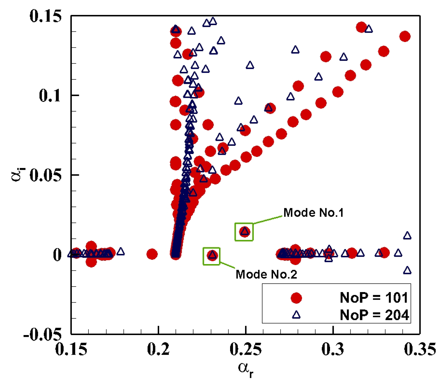The eigenvalue spectrum computed with the global method is illustrated in Figure 1.

By using two sets of computation grids with different grid spacing, two different discrete modes are identified and labeled as “Mode No. 1” and “Mode No. 2”, corresponding to the “Mode I” and “second mode” in one past publication [20]. The numbers and types of identified modes in general agree with the corresponding past results (Figure 6 in [20]). After globally arresting these two modes, a local computation scheme is applied to improve the eigenvalue accuracy. More accurate results for four modes were obtained, as listed in

Table 2. Discrete Modes of B.L. flow with and without Slip B.C.s, $Ma=4.5$, $R=1000.152$, $\Omega =2.2\times {10}^{-4}$, and x = 0.1393 m.

Case	Mode Names	${\mathit{\alpha }}_{\mathit{r}}$	${\mathit{\alpha }}_{\mathit{i}}$
No-slip	No. 1	0.2410054037	5.4910919074 $\times {10}^{-4}$
	No. 2	0.2307811189	−3.4244685299 $\times {10}^{-4}$
Slip	No. 1	0.2370296668	1.3886985577 $\times {10}^{-2}$
	No. 2	0.2324566444	−1.992537508 $\times {10}^{-5}$

. Mode No. 1 is stable with ${\alpha }_i>0$, and Mode No. 2 is unstable with ${\alpha }_i<0$.

Mode No. 2 is historically named the “Second Mack” mode. With the help of Plot Digitizer, the mode values of the past work [20] are read and presented in Figure 2 as comparison to the mode identification in the current work, for no-slip base flows. The differences in the final values are due to several reasons. First, the base flow computation schemes and results in the current and the past work are slightly different. This work adopts the self-similar solutions (evaluated with the shooting method) to the compressible flat plate B.L. flows; while Ma used Direct Numerical Simulation (DNS) [20] results. The exact solutions that we adopted are concise and elegant. By comparison, DNS can include more details and the results are more realistic, e.g., the temperature effects on viscosity and heat coefficients. However, limited information about their DNS treatments is available. Second, different G.E.s. for perturbations were adopted. The derived G.E.s in this work (available in Appendix B) are more comprehensive and accurate. As such, it is not surprising to see differences in the predicted mode values from the past results (Figure 6 in [20]). The modes presented in Figure 2 were computed with no-slip B.C.s. Mode No. 2 is the unstable mode and the corresponding fluctuations are expected to be stronger than those for Mode No. 1.

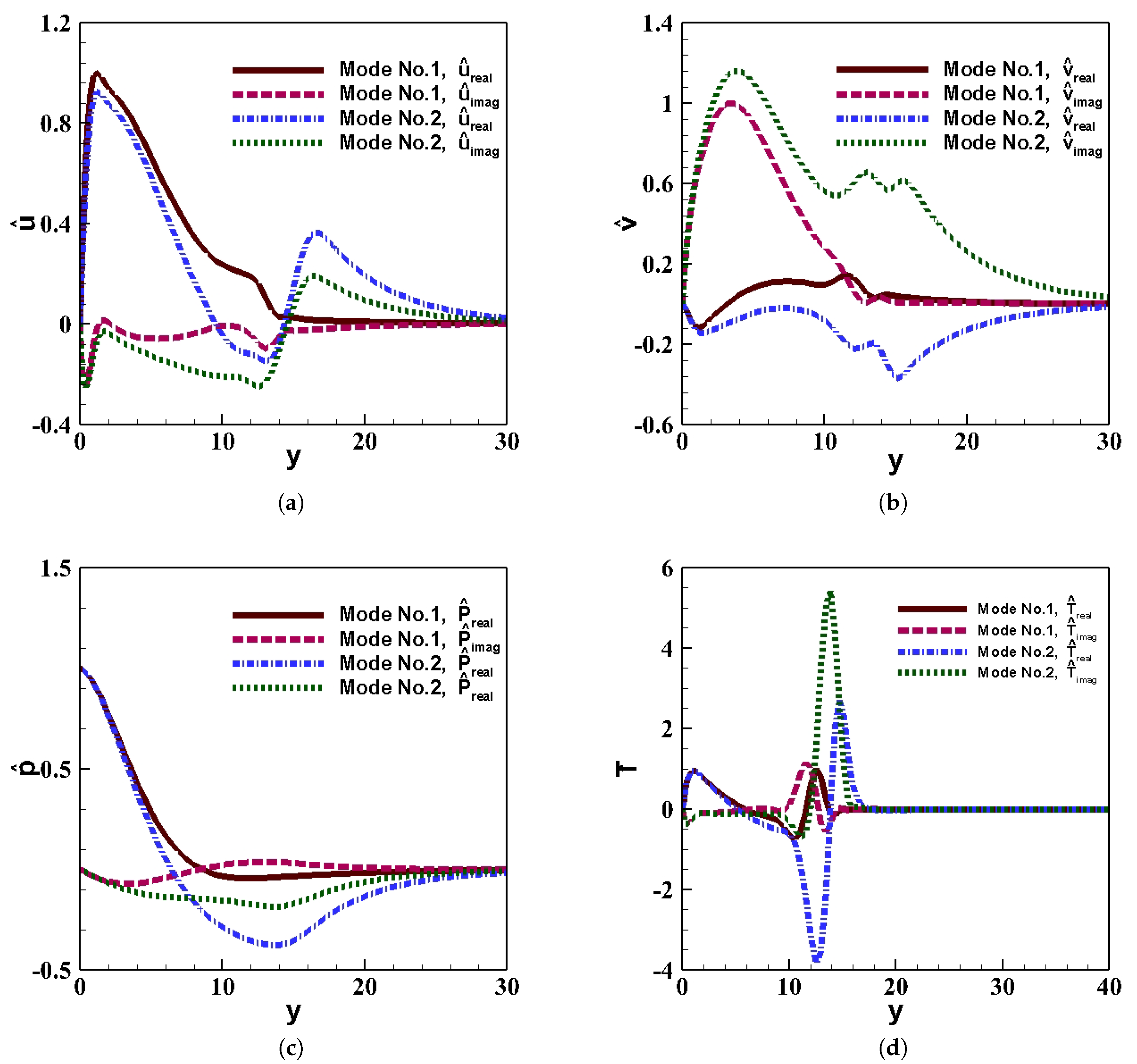
The eigenvectors at location $x^{*}=0.1393$ m are typical and shown in Figure 3. The plate surface B.C.s are not slip with a constant temperature.

The Y-axis in the above figure is normalized by the characteristic length $L^{*}=1.393\times {10}^{-4}$. The eigenvector $\widehat{u}$ is normalized by the no-slip ${\widehat{u}}_{real}$, $\widehat{v}$ by the no-slip ${\widehat{v}}_{imag}$, $\widehat{p}$ by the no-slip ${\widehat{p}}_{real}$, and $\widehat{T}$ by ${\widehat{T}}_{real}$. The B.L. edge has a thickness of $12.9L^{*}$. Figure 3a,b illustrates the imaginary and real parts of the eigenvectors $\widehat{u}$ and $\widehat{v}$ in Modes No. 1 and No. 2. Both imaginary and real parts of the eigenvectors in Mode No. 1 vanish within the B.L. However, Mode No. 2 has eigenvectors fluctuating outside the B.L. Because both show the characters of the unstable modes, they are expected to eventually break the base flow from laminar to turbulent as the perturbations propagate downstream. Figure 3c,d illustrates the pressure and temperature eigenvectors, $\widehat{p},\widehat{T}$, with similar behaviors to the velocity perturbations. The pressure perturbation is unnecessary to vanish at the B.L. edge; instead, for this situation, the largest pressure perturbation happens at the flat plate surface. The sub-figure at the right side is the temperature perturbation profile with the largest disturbances.

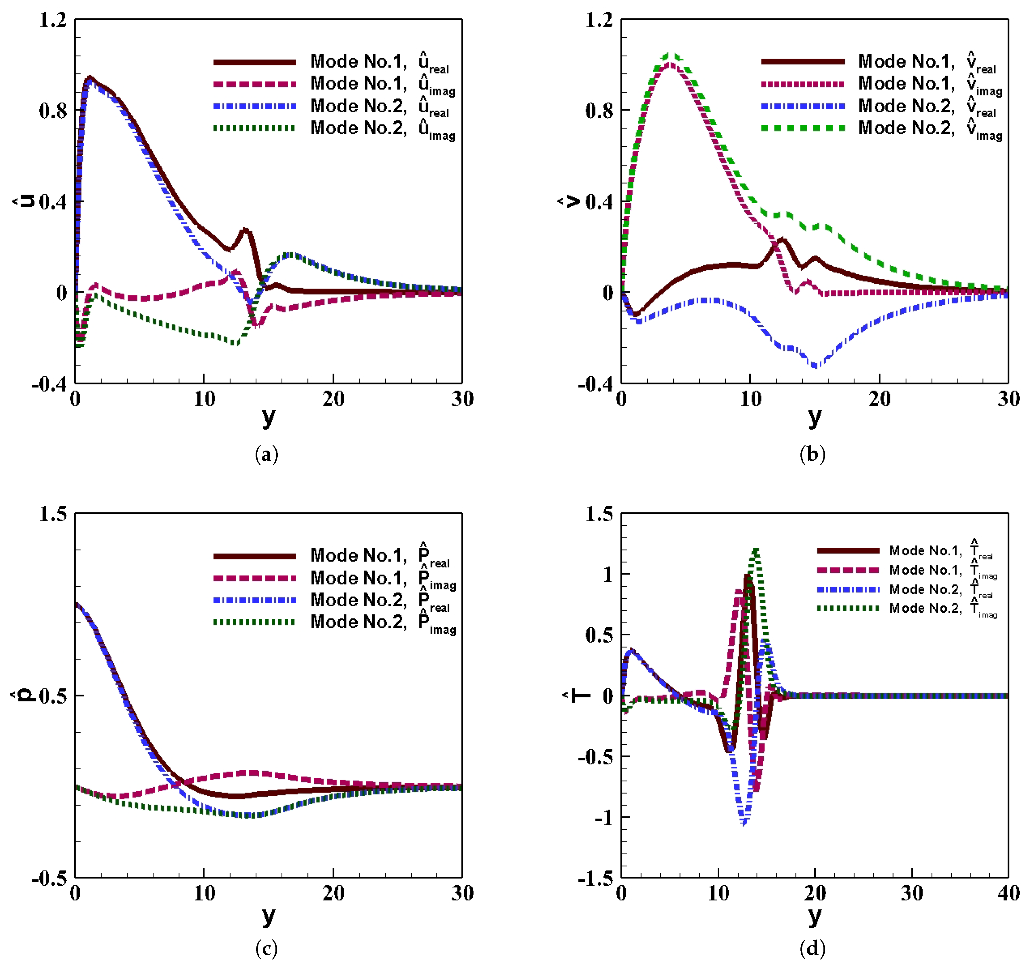
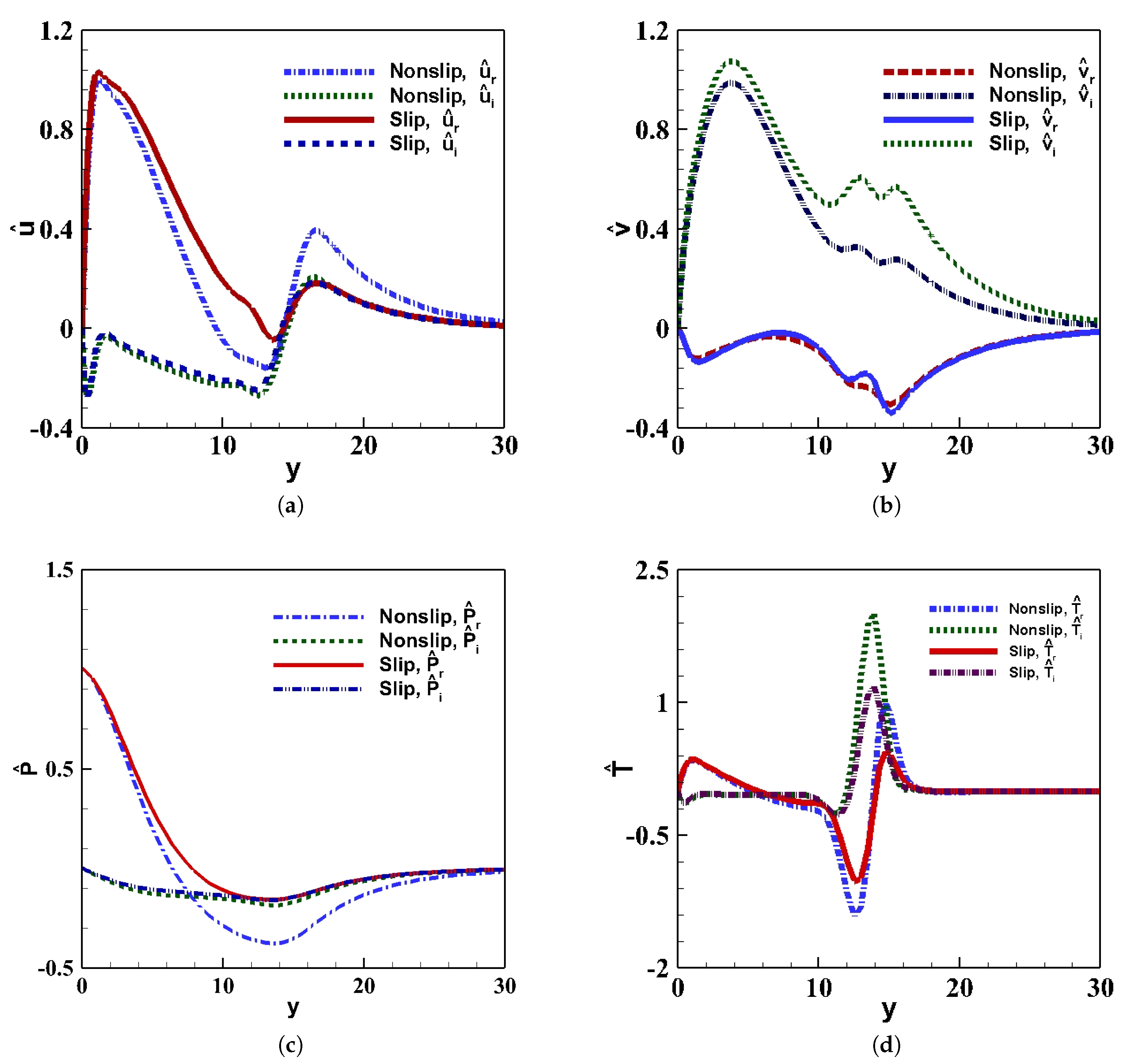
With the slip B.C.s, there are also two identifiable modes. One is stable and the other unstable. Figure 4 shows the corresponding eigenvectors of $\widehat{u}$, $\widehat{v}$, $\widehat{p}$, and $\widehat{T}$ for the slip flow. The slip B.C.s do not affect the number of identifiable modes in the no-slip B.L. flow. Meanwhile, the types of identified modes in the slip B.L. flows are consistent with the modes for no-slip B.L. flow as well. The corresponding eigenvectors (the two modes, and with both slip and non slip B.C.s., i.e. a total of four combinations) have similar profiles. They correspond to the unstable mode (Mode No. 2 has larger fluctuations than those for the stable modes).

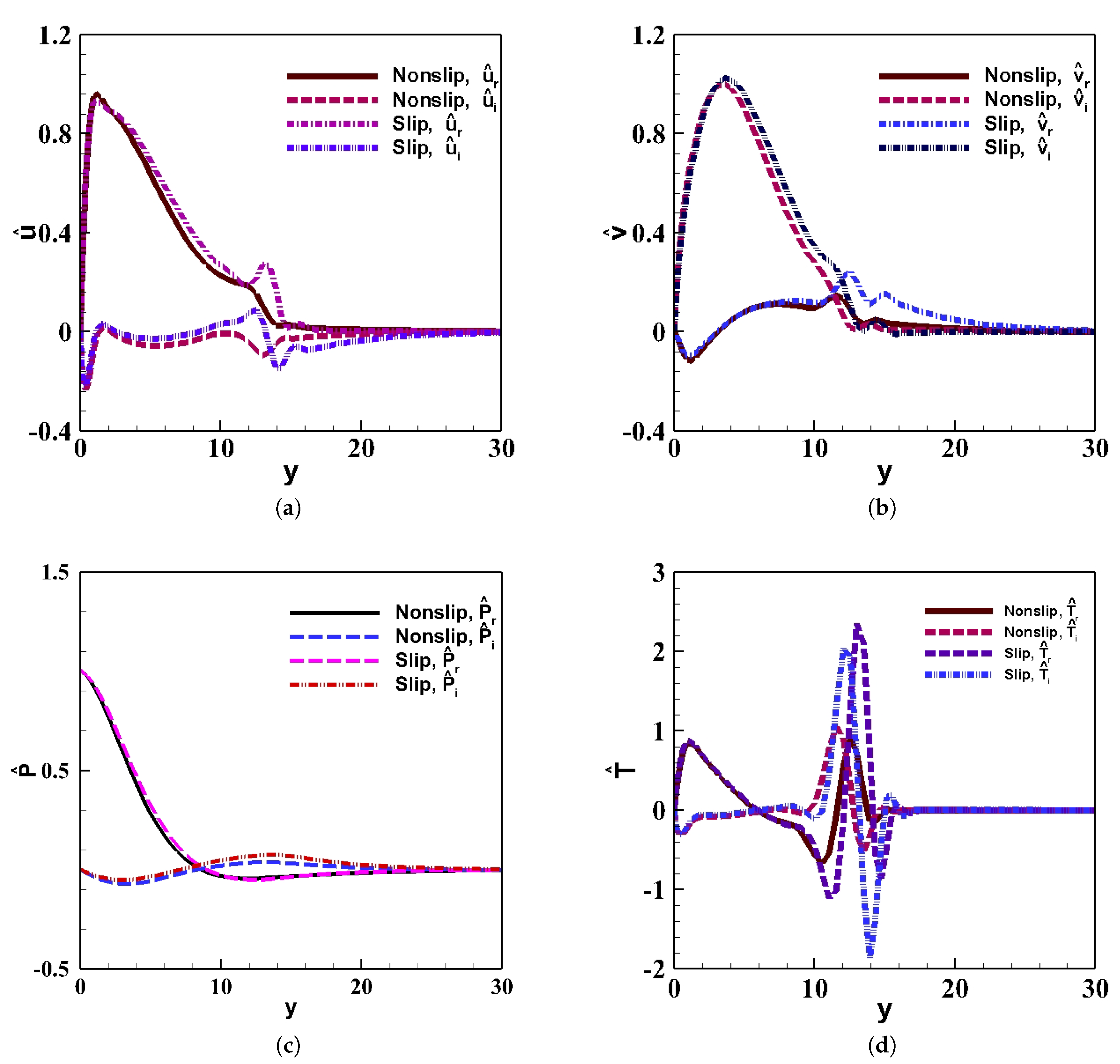
To visualize the slip B.C.s’ influence on the stable mode, Figure 5 presents Mode 1 related eigenvectors. The eigenvectors of the unstable mode (Mode No. 2) with slip and no-slip B.C.s are shown in Figure 6. When comparing the Mode 1 eigenvectors in Figure 5 and Figure 6, we can observe that the eigenvector fluctuations vanish within the B.L., and the fluctuations of $\widehat{u}$, $\widehat{v}$, and $\widehat{T}$ for both scenarios are similar. More smaller fluctuations near the B.L. edge of all eigenvectors are shown in the slip flow scenario.

However, considerable eigenvector changes are found in the slip flow scenario comparing to the no-slip scenario. The fluctuations of $\widehat{u}$, $\widehat{v}$, $\widehat{p}$, and $\widehat{T}$ with the slip B.C. scenario are smaller than their counterparts in the no-slip scenario. Slip B.C. enforcement intends to reduce the influence from the unstable mode on the base flow at the same flow station. This phenomenon indicates that, with the enforcement of slip B.C.s, the stable and unstable modes can be categorized differently. To further understand how the modes in the slip B.L. flow propagate upstream and downstream, mode tracking work was performed and the results are reported in the next section.

Mode Tracking Results

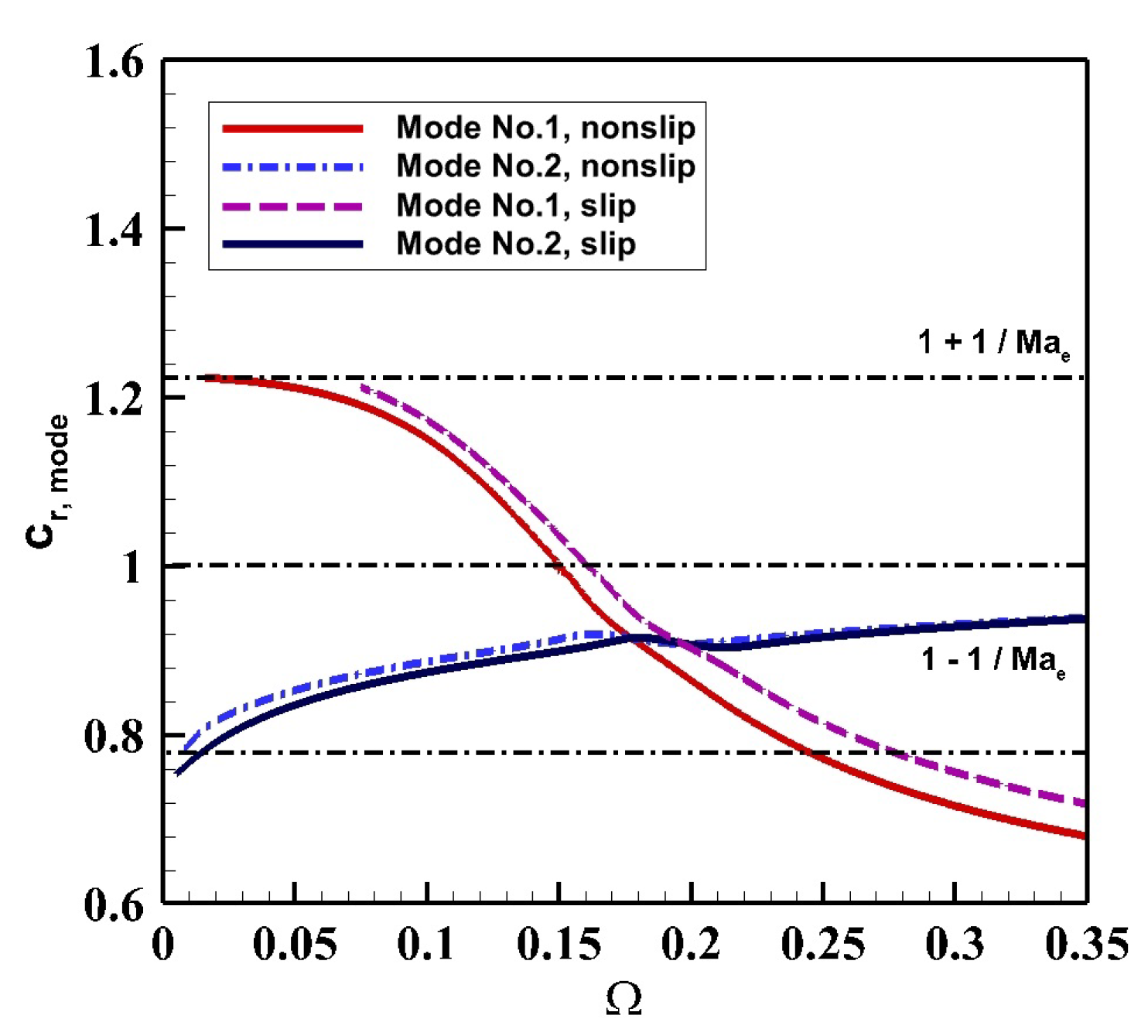
In both test cases, Modes No. 1 and No. 2 are tracked both upstream and downstream using $\omega =2.2\times {10}^{-5}$ at $R=1000.152$ as the starting point. Figure 7 illustrates the tracking results, based on the dimensionless mode phase velocity which is defined as:

$$c_{r,mode}=\frac{\Omega }{{\alpha }_r{U}_e}$$

(31)

where $\Omega =R\omega$. The changes of $\Omega$ can be achieved by increasing or decreasing the $R{e}_x$ with unchanged $\omega$ values, where again R = $\sqrt{R{e}_x}$. The simulations adopted a local $R{e}_x$ which means a smaller $R{e}_x$ represents an observing location closer to the leading edge. A larger $Re$ represents an observation station at further downstream. All the modes for slip and no-slip B.C.s are tracked upstream and downstream, the intruding wave frequency $\omega$ remains the same while R reduces to as small as $7.556\times {10}^{-4}$, and as large as $2.74\times {10}^6$. The mode is traced back to the upstream at an observing location $x=7.952\times {10}^{-13}$, which means the observing location range from 7.952 $\times {10}^{-13}$ m to 0.382 m. The fast acoustic wave line ($c_{r,mode}=1+\frac{1}{M{a}_e}$) and the slow acoustic wave line ($c_{r,mode}=1-\frac{1}{M{a}_e}$) are shown in Figure 7 as references and this figure indicates the dimensionless phase velocity behaves as a function of $\Omega$.

The no-slip B.L. flow mode tracking results are first analyzed. The intruding disturbance frequency is fixed at $\omega =2.2\times {10}^{-4}$. Mode No. 1 in the no-slip scenario is traced back to the starting point, the related wave is the fast acoustic wave with the phase velocity of $1+\frac{1}{M{a}_e}$ at the leading edge. The phase velocity continues to decrease when it propagates downstream. These characteristics distinguish this wave mode from Mode No. 2, whose phase velocity at the leading edge starts from the slow acoustic wave ($1+\frac{1}{M{a}_e}$). Resonance intersections of these two modes are shown at $\Omega =0.176$, which means they meet at a specific location where $R=802$ and $\omega =2.2\times {10}^{-4}$. At this intersection, Modes No. 1 and No. 2 share the same phase velocity. These results are very similar with the past results (Figure 7 in Ma’s work [20]). Due to different base flow conditions and G.E.s for perturbations, differences in the model values are expected but the results and mode tracking trends are very similar.

Compared with the no-slip flows, the mode tracking results of the slip B.L. flows share similar trends as they propagate downstream. The differences are evident. Neither Mode No. 1 nor Mode No. 2 is limited within the range of the fast and slow acoustic waves. Mode No. 1 has a higher phase velocity than $1+\frac{1}{M{a}_e}$ at the leading edge, and Mode No. 2 starts at the leading edge with a phase velocity slower than $1-\frac{1}{M{a}_e}$. The resonance interaction, in this case, happens at further downstream, compared to the no-slip B.L. flow scenario. Modes No. 1 and No. 2 intersect at $\Omega =0.193$ ($R=877$ at $\omega =2.2\times {10}^{-4}$). The intersection of these two modes is the “landmark” to distinguish the traditionally defined the first mode (T-S wave) and the second mode (Mack’s second mode) [2,20].

The first mode has been proven as the most dangerous mode for supersonic flows with specific oblique angles [38]. The delayed interaction between these two modes in the slip B.L. flow indicates an extension region for the existence of the T-S wave. It means with the same intruding disturbance frequency, the slip B.L. supersonic flow can be more unstable if the flow has specific oblique angles. The interaction delay also postpones the starting point of the Mack’s second Mode. The adoption of slip B.C.s delays the second mode’s instability until further downstream, compared to the no-slip B.L. flow.

Compared to a no-slip flow, Mode No. 1 of a slip flow always has a larger phase velocity when the waves propagate downstream. Especially after the resonance interaction, Mode No. 1 in the slip flow tends to propagate even faster. The phase velocity of Mode No. 2, on the other hand, behaves differently. It has a smaller phase velocity, compared to the no-slip scenario, while after the resonance interaction, the phase velocities of Mode No. 2 in slip and no-slip B.L. flow are almost indistinguishable. They propagate downstream with almost the same phase velocities.

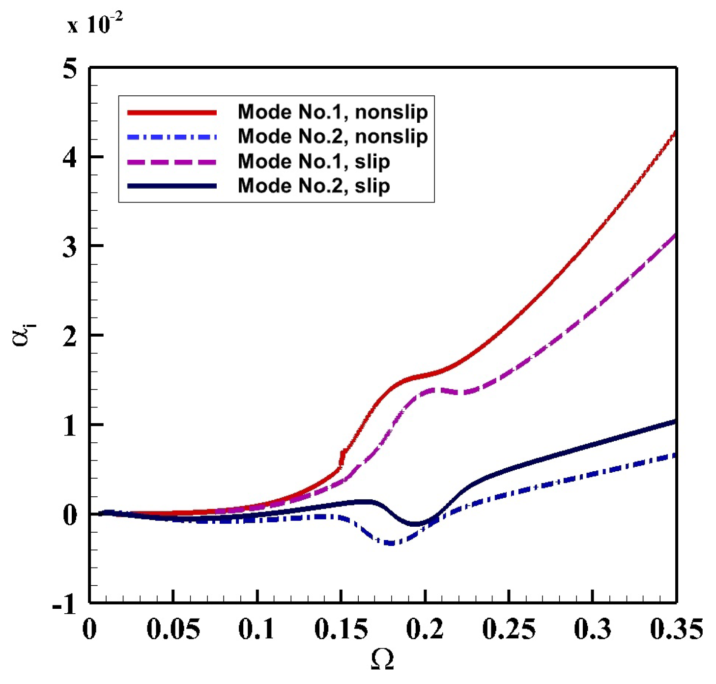
To further assist categorizing the modes, the distribution of the wave growth rates (${\alpha }_i$) as a function of $\Omega$ is shown in Figure 8. Modes No. 1 and No. 2 in both slip and no-slip B.L. flows are immediately categorized into the safe and dangerous modes. All four modes start with a zero growth rate at the leading edge. Mode No. 1 of the slip flow develops with a lower growth rate as it propagates downstream, compared to the same mode in the no-slip scenario. Modes No. 2 of both scenarios need to be discussed section by section. The dangerous wave region for the no-slip flow is $\Omega$ = [1.50, 2.18], and $\Omega$ = [1.75, 2.12] for the slip flow. Slip flows not only delay the onset of an unstable wave to further downstream, but also shorten the unstable wave range with respect to R at a fixed disturbance frequency.

Overall, comparing to the no-slip flow, incorporating the slip B.C. to the flat plate B.L. flow reduces the affected range with respect to R on the Mack’s second Mode instability. However, this B.C. can be more dangerous for supersonic flows with the T-S waves at specific oblique angles.

6. Conclusions

Velocity slip B.C. condition effects on flat plate B.L. flow stability were studied. First, a double-shooting method was introduced to obtain the base flow profiles with slip and a constant temperature boundary conditions at the plate surface. A relatively complete set of perturbation coefficients were derived. By utilizing LST over a supersonic B.L. flow with and without the slip B.C.s., we detected different discrete eigenmodes. For the case with no-slip B.C.s, two modes were detected and their values were compared with the past results in the literature. In general, the agreement was satisfactory with acceptable differences for several reasons. For B.L. flows with slip B.C.s, there are two modes detected as well. One is a stable mode and the other is unstable (Mack’s second mode). The eigenvectors of the stable modes in both slip and no-slip flows behave similarly. However, in the slip flow scenario, the eigenvector fluctuations corresponding to the unstable modes are appreciably smaller than the corresponding ones in the no-slip flow scenario.

The mode tracking results show that both the fast acoustic speed range for the no-slip stable mode at the leading edge, and the slow acoustic speed range for the no-slip unstable mode, the phase velocity are limited. As the stable mode develops downstream, the phase velocity slows down. On the other hand, the phase velocity increases for the unstable mode. The resonance phenomenon was observed for these two modes when their phase velocities reach the same value. After they synchronize, the stable mode becomes more stable and the unstable mode becomes more unstable. These results agree well with those in the literature for the scenario without slip B.C.s. For the slip flow scenario, the resonance location is delayed. The synchronization was not observed till a station further downstream. The Mack’s second mode’s instability is delayed in this case. Both the stable and unstable modes are not limited within the fast and slow acoustic wave phase velocity range, and this means these modes can be categorized differently. The delays of the resonance phenomenon also indicate that the slip B.C. in the flat plate B.L. flow can enlarge the T-S wave region. It further indicates that, with a changing oblique angle, the slip flow can be more unstable. The unstable mode for the slip flow has a region smaller than the corresponding one for the no-slip flow scenario, which means that the unstable mode onset is not only delayed by the slip B.C. enforcement but also shortened along the flow direction. The existence of the slip B.C. can delay the onsets of the conventional second mode (unstable mode) streamwisely. At the same observing location with a fixed intruding frequency, the slip flow scenario can be more stable than the no-slip flow scenario.