Cross-Correlation of POD Spatial Modes for the Separation of Stochastic Turbulence and Coherent Structures

Abstract

This article describes a proper-orthogonal-decomposition (POD) based methodology proposed for the identification and separation of coherent and turbulent velocity fluctuations. Typically, POD filtering requires assumptions to be made on the cumulative energy content of coherent modes and can therefore exclude smaller, but important contributions from lower energy modes. This work introduces a suggested new metric to consider in the selection of POD modes to be included in a reconstruction of coherent and turbulent features. Cross-correlation of POD spatial modes derived from independent samples is used to identify modes descriptive of either coherent (high-correlation) or incoherent (low-correlation) features. The technique is demonstrated through application to a cylinder in cross-flow allowing appropriate analysis to be carried out on the coherent and turbulent velocity fields separately. This approach allows identification of coherent motions associated with cross-flow transport and vortex shedding, such as integral length scales. Turbulent flow characteristics may be analysed independently from the coherent motions, allowing for the extraction of properties such as turbulent length scale.

1. Introduction

In the field of fluid mechanics, it is possible to obtain detailed, highly-resolved time-space velocity information from both experimental and computational approaches. Contained within these datasets are coherent structures and stochastic turbulence, often indistinguishable in raw velocity vector fields, the understanding of which is crucial in research and development. Coherent structures, often considered as vortices, are responsible for many flow phenomena, across many applications—lift, drag, mixing and heat transfer, for example. Similarly, an understanding of the turbulent characteristics of an aerodynamic system is vital in the study of many processes such as turbulent combustion. It is therefore important that these distinct structure classes be effectively identified and separated before further analysis may be carried out on each.

There have been multiple approaches suggested in literature to achieve velocity field decomposition. Ölçmen et al. [1] present a comparative analysis of suggested approaches—Reynolds decomposition (referred to as ensemble averaging in that study), proper orthogonal decomposition (POD) and frequency filtering amongst others.

Of these, Reynolds decomposition is the least computationally expensive to calculate and is often a useful first step in the analysis of a flow field. However, cyclic or oscillatory structures would be considered together with the turbulent field and therefore for many applications further decomposition is required. This is demonstrated by Stone [2] and Butcher [3] in the field of internal combustion engines, where there is a cyclic variation and a relatively increased frequency turbulent fluctuation both included within the fluctuating term which should be separated as in Equation (1):

$$U_i=\overline{U}+U_i^{\ast }+U{\prime }_i \left(= U_{true}+\epsilon \right)$$

(1)

where $U_i$ is velocity measurement, $\overline{U}$ is ensemble mean velocity and $U^{\ast }$ and $U\prime$ are coherent and turbulent fluctuations, respectively.

Frequency filtering, such as LES decomposition [4], applies a homogeneous filter to identify all structures above or below a cut-off scale allowing this separation. Using a priori knowledge of the flow field and expected structure sizes, the cut-off may be set such that coherent fluctuations, $U^{\ast },$ be filtering in (or out) as required.

POD is a commonly used technique in the fluid mechanics field for this purpose and will be the focus of this paper. The following subsection provides a background to the technique.

Proper Orthogonal Decomposition

Since its introduction to fluid mechanics by Lumley [5], the proper orthogonal decomposition (POD) technique has been widely adopted to identify coherent structures in flow fields. In the context of fluid mechanics, POD decomposes a velocity field into spatiotemporal modes according to Equation (2):

$$\left(x,t_i\right)={\displaystyle \sum }_{k=1}^M{a}_k\left(t_i\right){\phi }_k\left(x\right)$$

(2)

where $u$ is the velocity, $M$ is the number of modes, $a_k$ is the temporal coefficient and ${\phi }_k$ is the eigenmode (or spatial mode). In the determination of spatial modes, ${\phi }_k,$ it is commonly accepted that the classical method [6,7] is inefficient for typical PIV datasets—where the number of spatial locations is significantly greater than the temporal steps—and therefore the ‘snap-shot’ method is used [8]. The modes are then typically arranged according to their energy content, i.e., the associated eigenvalue.

For the reconstruction of velocity fields, it is possible to consider a reduced order representation of velocity if the number of POD modes; $M$ is less than the total number of snapshots. This is a commonly employed technique for filtering velocity field data. If the number of POD modes for the reconstruction is equal to the number of snapshots in the original dataset, then the reconstructions would be exactly equal to the original snap-shots. Therefore, the methodology for the selection of $M$ is integral to the analysis process—as it defines how much information is represented.

The most commonly used criteria for determining a cut-off value, $M$, are based on the cumulative energy threshold [9], E, defined in Equation (3):

$$\frac{{{\displaystyle \sum }}_{k=1}^M{\lambda }_k}{{{\displaystyle \sum }}_{k=1}^T{\lambda }_k}>E$$

(3)

where T is the total number of snap-shots in the original data and $\lambda$ is the mode eigenvalue.

Defining the cut-off mode in this manner allows a total fraction of the energy desired in the reconstructions to be considered—meaning that only the most energetic structures and fluctuations are considered. Typically, 90% is used for the cumulative energy threshold [8,9], but the subjective user-defined, arbitrary nature of the criterion has led to a range of values being defined in literature between 75 and 90%. Physically, by limiting the amount of energy included in the reconstructions, desired information may be inadvertently excluded, particularly in cases with high levels of turbulence and/or when that energy is similar to periodic or cyclic fluctuations as is the case, for example, in internal combustion engines in-cylinder flow [3,10]. In addition, defining the cut-off based on energy may increase the susceptibility to corruption by erroneous velocity vectors with large magnitude and therefore large energy value, if these have not been successfully removed prior [11].

The corruption of higher energy modes by erroneous vectors is highlighted by Epps and Techet [11] who suggest the consideration of the root mean square (RMS) stating that only those modes whose RMS velocity exceeds that of the underlying PIV measurement RMS should be considered. Raiola et al. [12] propose that the POD spectrum instead be optimised based on the comparison between the POD eigenvalue decay rate and the turbulent spectrum in Fourier space, defining the cut-off mode, $M$ according to Equation (4):

$$M= {\left(\frac{Tq}{{\sigma }^2\xi \left(5/3\right)}\right)}^{\frac{3}{5}}$$

(4)

where q is the average turbulent kinetic energy (TKE) over all spatiotemporal data and $\xi \left(s\right)$ is the Euler–Riemann zeta function. Brindise and Vlachos [9] propose the combination of discrete cosine transform (DCT) and Shannon entropy to define which modes should be considered. A significant difference in this approach is that the modes are re-ordered by entropy before a cut-off is defined. This allows for some low order modes which may be corrupted by erroneous vectors to be disregarded, irrespective of their surrounding energy-ordered POD modes.

A novel approach to defining the cut-off is employed by Doosttalab et al. [13]. In the study of a bio-inspired coating on an airfoil, the cut-off is determined by considering the streamwise auto-correlation. An iterative approach is used, increasing the cut-off and comparing the zero-crossing point of the streamwise auto-correlation from the pre-cutoff estimation and the original data. When this occurs at the same location, this mode number is used. It is worth noting that, using this approach, the authors observed a cutoff of 532 from a possible 4000 modes. This is significantly larger than the cutoff values typically referenced elsewhere in literature.

2. Methodology

The literature presented thus far highlights the criteria commonly used for the selection of POD modes. The methodology presented in this paper provides an alternative approach to defining which POD spatial modes are associated with the coherent motions, and which represent flow features representative of turbulence.

The methodology is underpinned by considering a pair of repeated experiments under similar conditions. In this situation, it would be expected that when considering flow statistical measures, the two sets of results would be highly similar, albeit with some stochastic variation evident in the comparison of instantaneous flow fields. Further, performing decomposition, POD, independently on each set of results would result in similar spatial modes representing the coherent motions; with a similar number of POD modes comprising the turbulent energy content of the flow for each experiment. Therefore, by the comparison of these independently calculated POD spatial modes from each result set, it may be deduced that those spatial modes that appear in both sets contain coherent flow information. In addition, the stochastic nature of turbulence suggests that there should be no similarity in the spatial modes, other than the number of modes and the total flow energy proportion that they represent.

Building on this concept, the presented identification technique allows a new definition of coherent and stochastic turbulent parts of a single set of velocity vector field to be separated for further analysis as required. This is achieved by generating two sets of POD modes each based on half of the original set of velocity fields. The process will be described in detail by application to an experimentally obtained dataset. The details of the experimental setup are given in Section 2.1, and the identification technique is described in Section 2.2.

2.1. Experimental Setup

The dataset to be used for demonstration of the identification methodology is an example of the cross-flow behind a cylinder—a case which is well studied in literature [14,15]. For this study, flow fields are experimentally obtained using planar image velocimetry (PIV) in the Loughborough University (LU) horizontal water flow tunnel facility, depicted in Figure 1. The test piece is a single 1” (25.4 mm) diameter, D, brass cylinder which is placed within the 0.3 m × 0.37 m working section, spanning the full height. The blockage co-efficient (diameter width) was 0.069. Further design details of the tunnel may be found in literature [16]. Upstream velocity, $U_0=0.302$. m/s, giving a Reynolds number based on cylinder diameter, $Re=8600,$ i.e., turbulent flow.

Water PIV measurements were made in the mid-height plane, 0.15 m, (as indicated in Figure 1) immediately downstream of the test piece in a region covering 0.12 m × 0.12 m using well-mixed 20 µm polyamide seeding particles. A new Wave Pegasus 527 nm laser provided illumination of 10 mJ/pulse at 1 kHz. A single Photron APX 1MP camera, operating at 1 kHz, was used to capture PIV images. All timing, synchronisation and vector field processing was controlled and carried out using LaVision hardware, PTU8 and software, DaVis v7. A Multi-pass, reducing size interrogation window strategy was used on the image pairs to produce 2-component, 2-dimentional (2C2D) vector fields. Interrogation windows for initial passes were 64 × 64 with 50% overlap, with two subsequent passes at 32 × 32, 50% overlap. The resulting temporal and spatial resolutions were 1 kHz and 1.905 mm × 1.905 mm respectively. Flow was set according to an upstream, streamwise velocity of 0.3 m/s. Measurements show that the average velocity was 0.302 m/s in the streamwise direction. Upstream RMS velocity was also assessed for both streamwise and cross components and was 0.004 m/s and 0.003 m/s respectively.

It should be noted that in the experimental testing, an optical aberration was present around the center line, in the region of X = 45–60 mm. This was a result of an imperfection on the tunnel wall which caused a lens/blurring effect over a small, localized area. This is not visible in ensemble average (Figure 2b), instantaneous or decomposed figures. However, it is considered that the data in this area would not be reliable in the calculation of higher-order statistics and frequency content. Therefore, this has been masked from all subsequent presented figures, and the region has not been included for any of the presented analysis.

2.2. Flow Characteristics

An example of instantaneous flow and the ensemble average is presented in Figure 2a,b respectively, with the cylinder placed at (0,0). Throughout the paper, distance is non-dimensionalised by the cylinder diameter.

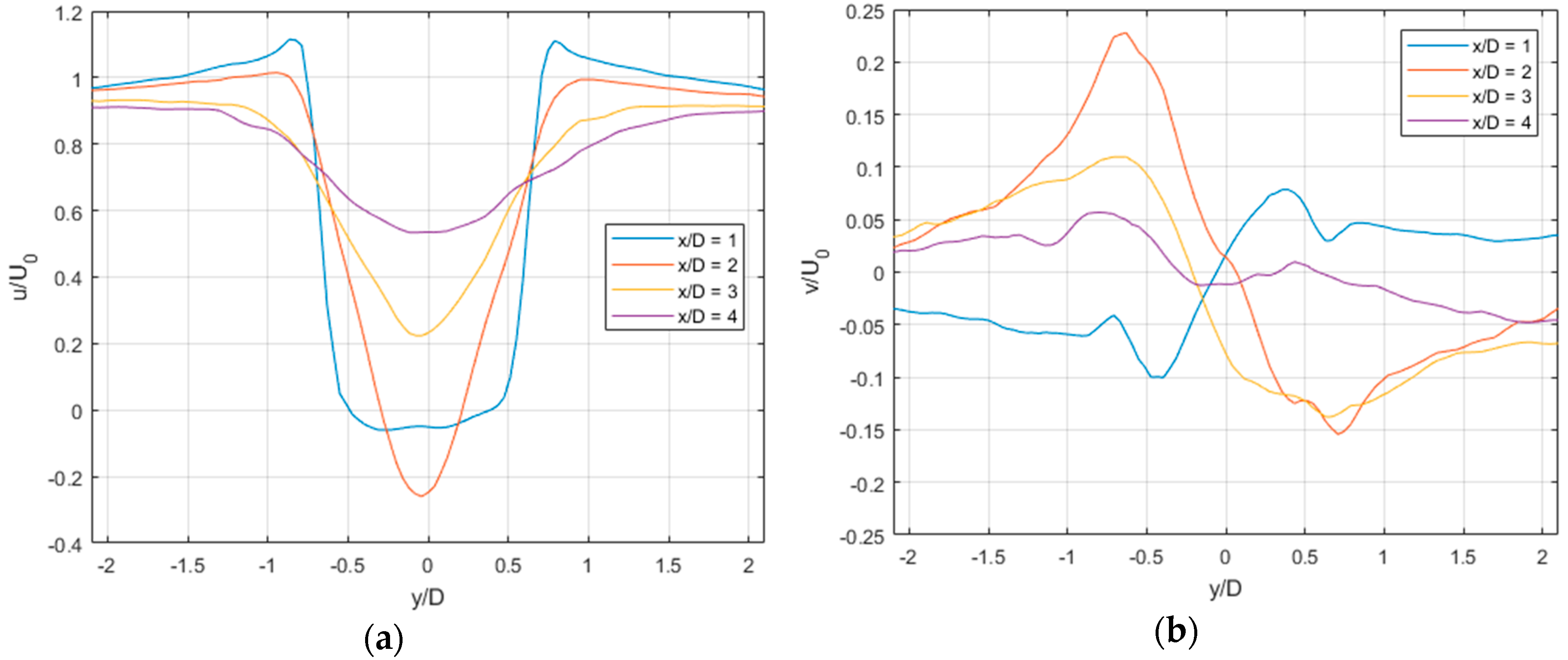
The flow exhibits a counter-rotating vortex pair immediately behind the cylinder, visible in the ensemble average. Free-stream regions exist either side of a central turbulent region, with a slight bias in the negative y-direction, as further evident in the profiles presented in Figure 3.

There is little fluctuation in the free-stream area, as evident in the velocity RMS presented in Figure 4, indicating low turbulence in this region. As the ensemble average is removed prior to POD analysis as is convention, it is expected that many of the POD modes will contain information relating to the central region.

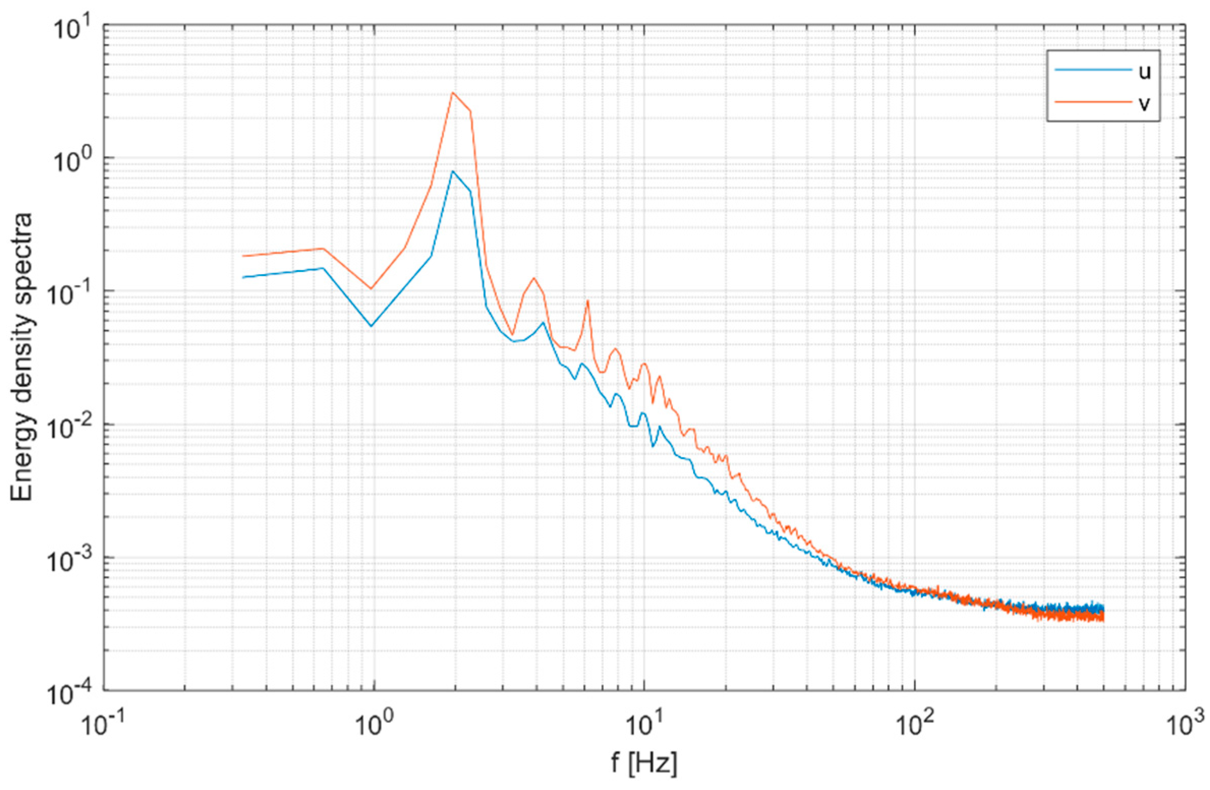
Analysis of the velocity frequency content, presented in Figure 5, reveals a peak at between 1.953 Hz and 2.279 Hz. The true peak appears to be located between these values, with the resolution limited by the duration of the measurement.

The frequencies correspond to a non-dimensional Strouhal number in the range 0.164–0.192 calculated according to Equation (5). This is related to the vortex shedding that occurs in this flow case, agreeing with reported studies in literature, for example, Perrin et al. [17,18]. In that work, flow past a cylinder in a wind tunnel is studied, with a peak frequency of 22.5 Hz observed (in air flow), corresponding to a similar Strouhal number of 0.21.

$$St=\frac{fD}{U}$$

(5)

2.3. Identification Methodology

Firstly, it should be determined that the dataset is of sufficient size (N) to adequately represent the flow features using half of the time instances captured (N/2), ordered randomly. This may be effectively assessed by considering the convergence of statistics between the two half-datasets (set A and set B) and the full dataset such as a comparison of the rms velocity component distributions. Figure 6 demonstrates parameters that may be used to assess the suitability of the number of snapshots considered. Here, the order has been randomised and the mean velocity distribution for a given number of snapshots is compared with the population mean and the velocity error, $\epsilon$, the difference between population mean velocity at each point and the mean velocity at each point for a given number of snapshots, is evaluated by a PDF. Figure 6a presents the PDF for 1536 (i.e., half of the dataset) snapshots error from which the standard deviation may be extracted.

Further, if this process is repeated from 1 up to the number of available snapshots, the trend may be plotted as in Figure 6b. It can be seen that after a modest number of snapshots, the error is less than 0.01 magnitude, and by 1536 it is approximately of magnitude 0.001 which in this case is deemed to be acceptable. In addition to this check, the velocity RMS Figure 6c for a given number of snapshots can be seen to converge after approximately 1000 snapshots. Therefore, it is deemed that using half of the dataset, 1536 snapshots may sufficiently represent the full dataset.

Whilst here it has been determined that N/2 vector fields are sufficient, this may not always be the case; this would depend on many factors including the frequency of both the large-scale flow structures and the measurement.

Once it is determined that both set A and set B are statistically similar to each other, and to the full dataset, POD analysis may be performed on each set independently. Following decomposition according to Equation (2), two sets of POD spatial modes should exist, allowing a comparison between them.

Following conventional POD processes, the energy contained within each mode may be calculated according to Equation (3) and examined. This is calculated for set A and B and presented in Figure 7. Both sets provide a similar distribution of energy with the first two modes for each containing the majority of flow information. This indicates that much of the large-scale, dominant flow structures are captured by these modes.

It should be noted that during the application of the POD approach, the ensemble average is first subtracted. This is because it would otherwise appear as the first, most energetic mode, sometimes referred to as mode 0 in cases where it is not removed prior to POD analysis. Therefore, the decomposition is only carried out on the fluctuating velocity component. The mean is later recombined in the reconstruction.

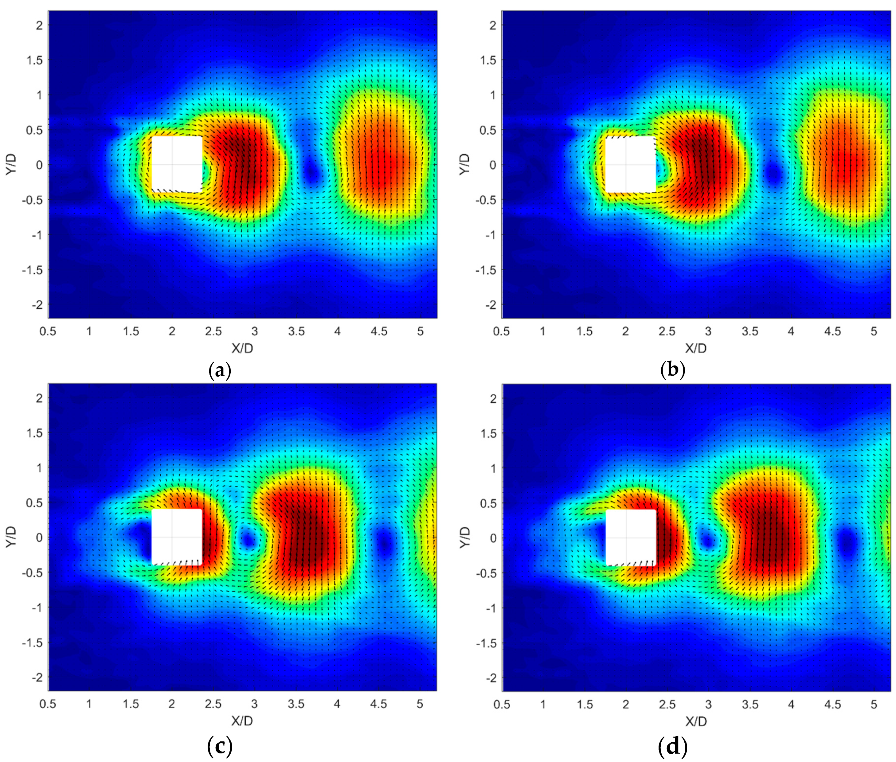
As previously discussed, one method for determining the cut-off mode between coherent and turbulent motions is to consider the energy knee-point, which using Figure 7 would suggest mode 3. However, there may be subsequent modes which still contain coherent motions, but at lower energy. Considering the first three modes only, Figure 8 presents the associated spatial modes obtained from each of the two sets. Firstly, there is clear evidence from Figure 8e,f that visually similar spatial modes are obtained for the third mode in both sets, which would indicate the likelihood of good correlation and therefore imply that these modes are representative of coherent motions and therefore should be considered as such.

Examination of both the energy content, Figure 7, and the spatial mode distributions, Figure 8, for modes 1 and 2 suggests that there is a pairing between them. Pairs of modes often exhibit very similar energy as is the case here, when their pairing is descriptive of oscillatory behaviour. By exploring the temporal coefficient information, this pairing can be further characterised. Firstly, Figure 9a presents the first two modes plotted against each other, revealing the pairing dependence of these two modes. Considering the frequency content of the temporal coefficients in Figure 9b reveals strong evidence that the oscillatory pairing is actually that which is responsible for the same frequency peak at approximately 2 Hz identified earlier. For comparison, the frequency content of mode 3, a₃ is also plotted, exhibiting similar frequency energy distribution across the frequency range, outside of the 2 Hz peak.

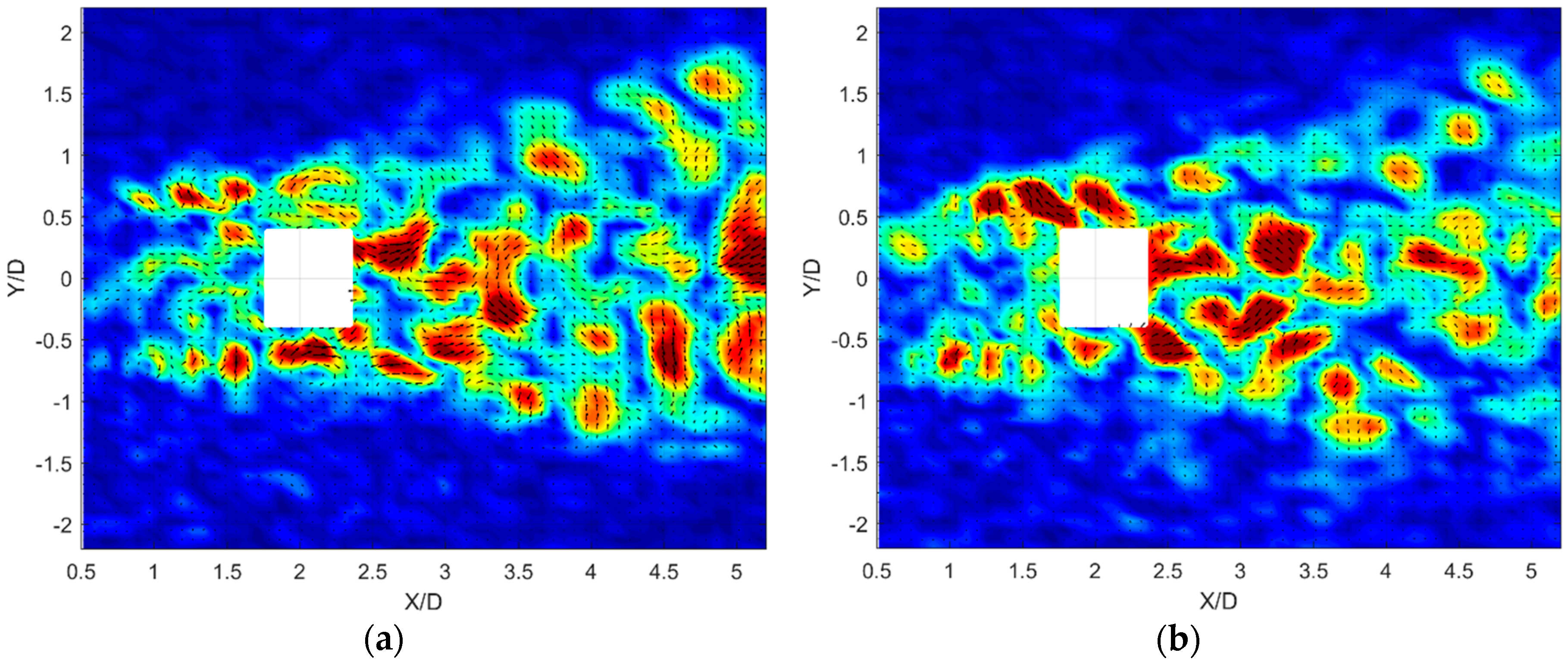
Now, considering higher order modes, which are not expected to be representative of coherent motions, Figure 10 presents POD spatial mode 30 for each set. In contrast to those modes presented in Figure 8, there is no clear visual similarity between the two POD spatial modes. This indicates that the two presented modes are not representative of coherent motions. However, if the size of the structures represented in each mode is considered, these are of similar character and of an expected magnitude for turbulent length scales in this flow. Further, the region in which the POD spatial mode structures are contained is within the central, turbulence containing region, with insignificant contributions in the free-stream area.

Similarity between two flow fields—or in this case spatial modes represented as velocity vectors—may be achieved by considering two-point statistics, specifically the cross-correlation function.

The generalized equation for the cross-correlation function between any two-points separated by the vector, r and time τ may be defined as:

$$R_{ij}\left(x,\mathit{r},\tau \right)=\frac{\langle u_i\left(x,t\right)u_j\left(x+\mathit{r},t+\tau \right)\rangle }{\sqrt{\langle u_i^2\left(x,t\right)\rangle }\sqrt{\langle u_j^2\left(x+\mathit{r},t\right)\rangle }}$$

(6)

where u_i and u_j are the velocity components for correlation. It is common to use a simplified form of Equation (6) for correlations at the same point in time, spatial velocity correlation (SVC, τ = 0) or correlations performed at the same point in space, autocorrelation function (ACF, r = 0). For the application presented, it is the cross-correlation of POD spatial modes that is to be considered, thus no true time association exists. However, for the purposes of the comparison, it is convenient to consider the two desired POD modes for comparison as two time-steps at the same spatial location, leading to the following equation:

$$R_{ii,AB}=\left|\frac{\langle u_i{\left(x\right)}_A{u}_i{\left(x\right)}_B\rangle }{\sqrt{\langle u_i^2{\left(x\right)}_A\rangle }\sqrt{\langle u_i^2{\left(x\right)}_B\rangle }}\right|$$

(7)

where subscripts A and B define the POD mode from set A and its corresponding (or other as appropriate) POD mode from set B respectively.

Each mode number is considered in turn from mode 1 through to the total number of spatial modes available in each of the two datasets. For each spatial mode, the surrounding +/−5 modes may also be compared. For example, S_A = 10 will be compared using Equation (7) to modes S_B = 5:15. This is to account for any minor re-ordering of POD modes which can occur when two or more consecutive POD modes have similar energy and therefore may be slightly re-ordered during the calculation of eigenvalues. This leads to a set of (11) correlation values for each mode considered, as represented in Figure 11. It should be noted that the absolute correlation should be considered as it is possible for two POD analyses of nominally the same velocity fields to produce an equal but opposite velocity spatial mode, with the corresponding reversed temporal co-efficient.

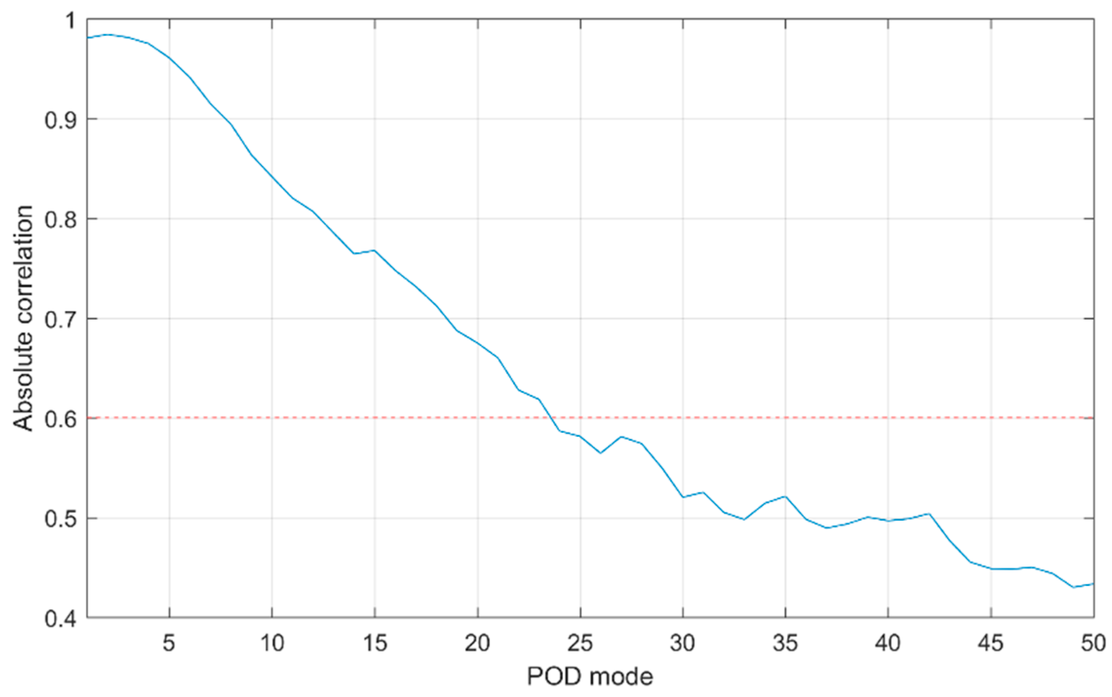
It can be seen in Figure 11 that for the majority of modes in set A, the strongest correlation occurs with the corresponding mode in set B as one would expect. However, there is evidence of some mode re-ordering, for example, for the modes 18 and 22 where the strongest correlation occurs with a mode +2 and −2 respectively, showing evidence of a pair with similar energy whose order has been swapped. Following this approach, the most significant correlation value is extracted for each mode in set A to obtain Figure 12. For the purposes of selecting a cut-off mode, it has been deemed appropriate to smooth the trend to easier identify the point at which POD spatial modes have poor self-correlation. The reasoning is that in turbulent fields, with similar sized features, spikes of increased correlation may be observed for a single spatial mode. In addition, in consideration of correlation in Figure 12, it is necessary to define a value below which it is considered poor correlation. The introduction of this new parameter, R, allows tuning of the coherent structures to be included in the low order model. In this case, 0.6 is selected as the threshold to poor correlation.

From Figure 12, it is apparent that poor correlation (defined here as less than 60%) occurs at greater than 23 POD modes for the datasets presented. Therefore, it follows that the first 23 modes contain high levels of coherent information and should therefore be considered when POD filtering is applied to these velocity fields. Subsequent analysis of coherent structures and their characteristics may be carried out on a reconstruction using the first 23 POD modes. Analysis on stochastic turbulence characteristics of the flow should be carried out on a reconstruction using the remaining 24-1536 POD modes (otherwise known as the residual fields). At this point, it would be possible to instead only consider the modes which have a significant correlation.

The final step of the technique is to recombine the POD spatial and respective temporal co-efficients to obtain coherent and turbulent velocity fields. The cut-off POD mode should be used (in this case 23) for the reconstruction of coherent fields of each dataset, S_A and S_B. The two datasets may then be recombined, taking note of the randomization carried out earlier in the presented methodology. This is particularly important if subsequent frequency analysis of coherent structures is to be carried out.

The resulting decomposed flow field provides a coherent and incoherent part of each instantaneous velocity field as presented in Figure 13a,b respectively. The original, raw velocity field is also presented in Figure 13c. The effect of reconstructing the velocity field using only the POD modes associated with coherence is a smoothed velocity distribution which still contains the larger, bulk features without the small-scale structures—this is visually evident in a direct comparison between Figure 13a,c.

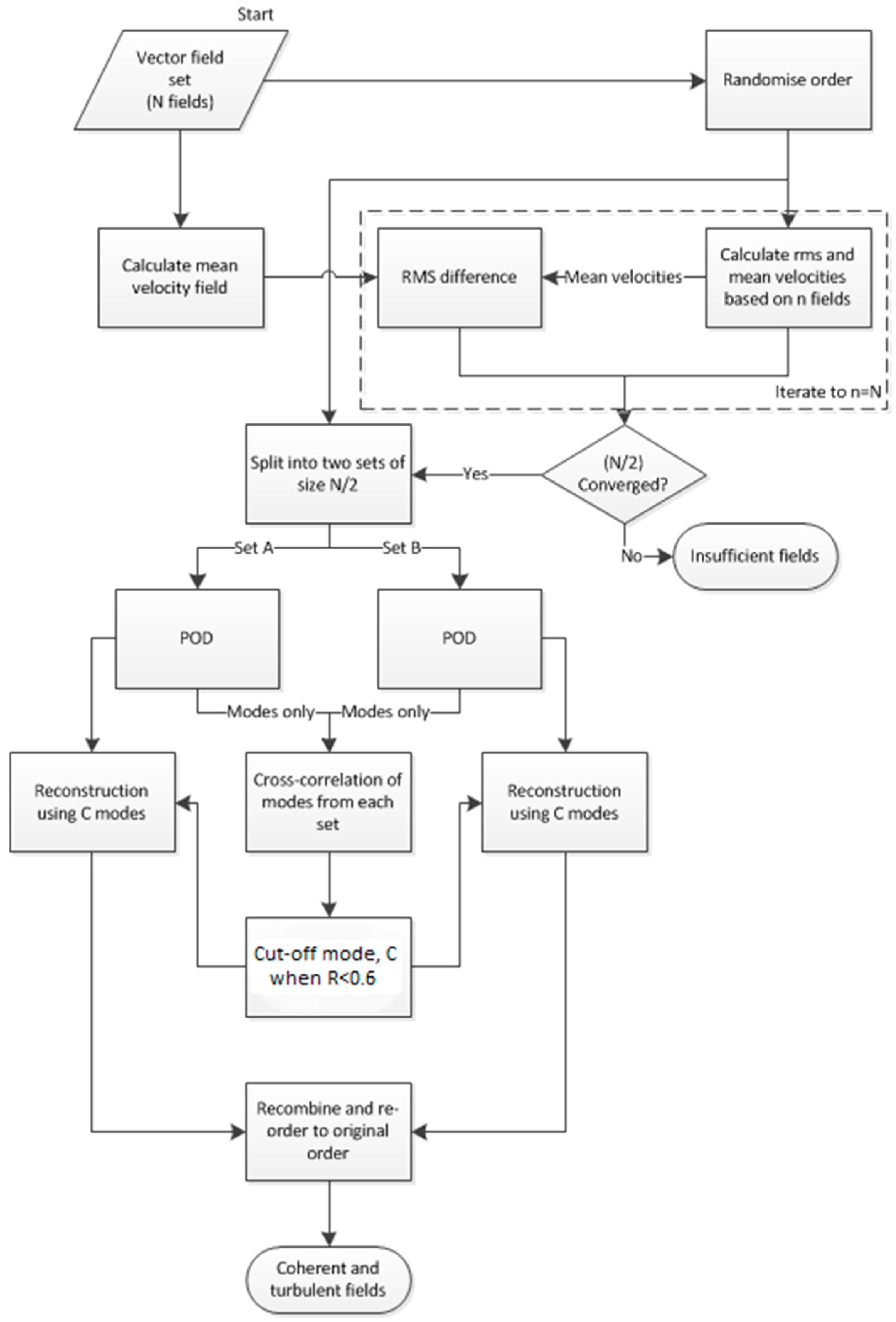
The entire process is summarised as a flowchart in Figure 14 which should be followed for implementation with any new dataset. It is possible to omit some stages such as the check for convergence, if desired.

3. Analysis of Separated Velocity Fields

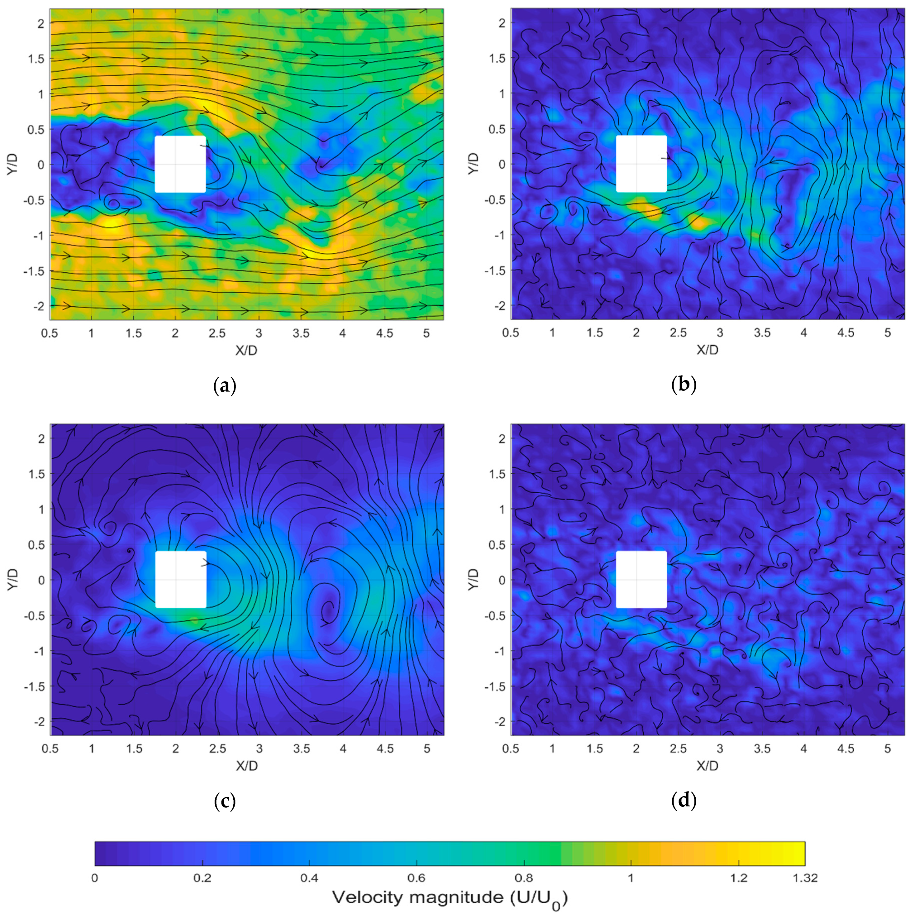
Once the velocity vector distributions have been reconstructed and re-ordered in the original order, analysis of coherent structures and turbulent parts may be carried out separately, as appropriate. Figure 15 presents an example instantaneous flow field, with each of the possible decomposed velocity fields. Figure 15c,d are the results of the presented methodology, representing coherent and turbulent parts respectively.

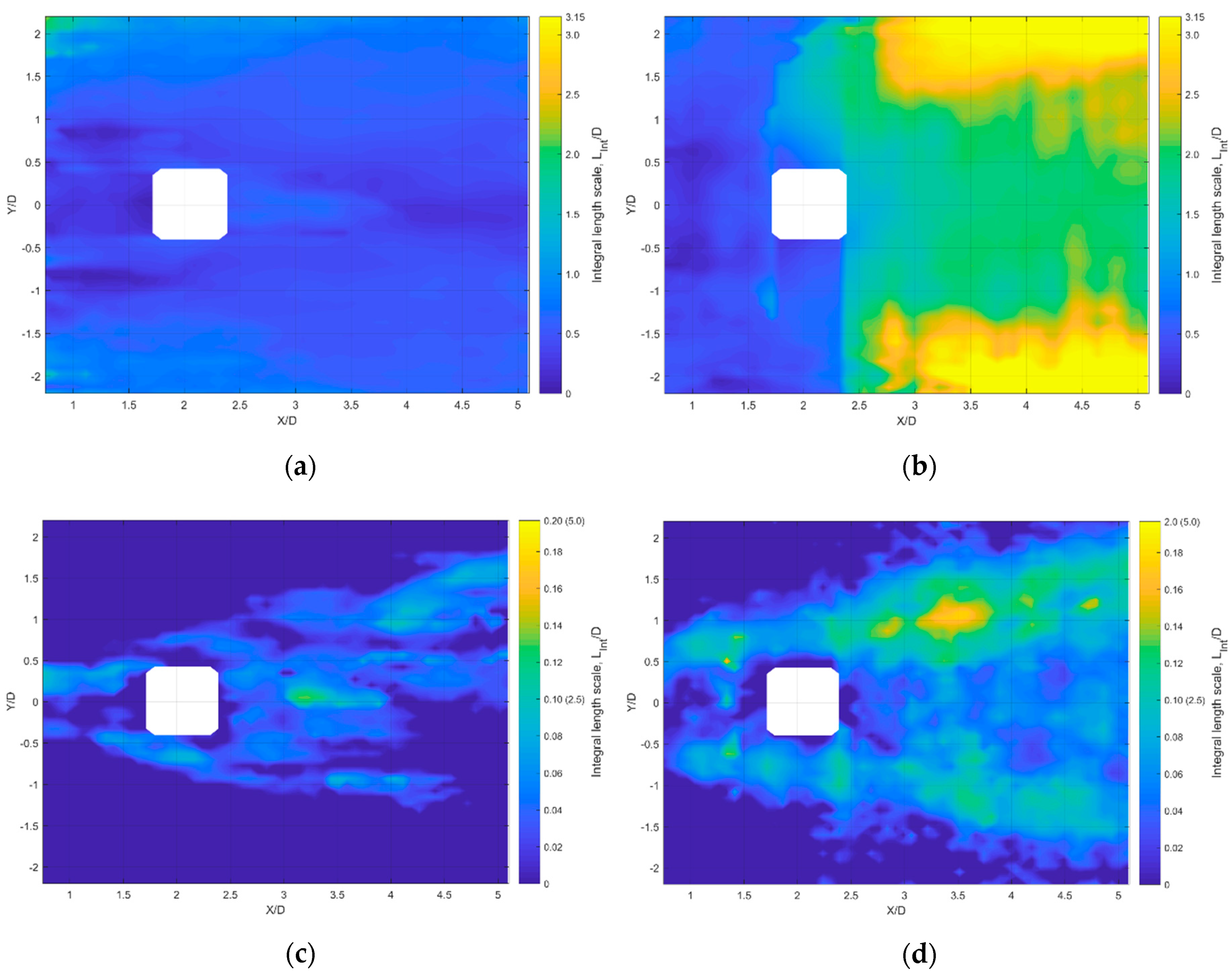
For reference, Figure 15b presents the Reynolds decomposed fluctuations, which are equal to the sum of the fields in (c) and (d). However, the purpose of presenting the Reynolds decomposed field is to illustrate that visibly, the large-scale motions are evident, but it is difficult to make quantitative evaluation due to the inclusion of turbulence. Considering the coherent fluctuating motions only, Figure 15c, these may be characterised by large vortices responsible for the bulk transport in the y-axis direction. The structures lead to relatively large integral length scales associated with the coherent part, as is evident in Figure 16a,b. The inhomogeneous distribution of length scales is influenced by the presence of these structures with values in the region of ¹L₁₁ = 22 mm and ²L₂₂ = 50 mm in the surrounding region (approximately 1–2 D), compared to a field average length scales of 15 mm and 42 mm respectively. Further, there is a clear link between these structures, and the first two POD modes presented in Figure 8a,c (or Figure 8b,d), underlining the dominance of these modes as expected from the significant energy contained within, as demonstrated in Figure 7. It should be noted that having a masked region within the flow has an impact on the calculated length scales, particularly where these are particularly large. This is most evident in Figure 16b; here, it is not possible to calculate the length scale immediately below the masked region as it is expected to be larger than the distance between the masked region and the edge of the domain. This strip of data should not be regarded any further in analysis. However, in the case where the integral length scale is much smaller, for example in the turbulent field, Figure 16d, there is no evidence of this artifact.

Similar analysis of integral length scales of the turbulent field, presented in Figure 16c,d reveals a distribution with substantially smaller associated length scales of 1.5–3.5 mm (approximately 0.1 D). The length scale distributions show how only the wake region contains significant turbulence, as one may expect, with little evident in the freestream area.

It is commonly acknowledged that the velocity and velocity gradient distributions should conform to a Gaussian distribution in the case of stochastic turbulence. It is therefore expected that a study of these parameters in the incoherent decomposed velocity fields presented will exhibit the characteristics of turbulent flow. Figure 17 presents the bivariate distributions for u and v velocity components for each of the considered velocity sets.

Firstly, if the original velocity data is considered in Figure 17a, there is evidence of a strong bias as would be expected in the direction of the freestream velocity (i.e., positive u), peaking at close to u/U₀ = 1, the mean upstream velocity. Performing Reynolds decomposition effectively removes this bias, as demonstrated in Figure 17b. While the peak is now centered close to (0,0), the spread is much greater in the cross-flow direction, v, compared to streamwise due to the shape of the large (coherent) structures that can be seen to dominate, for example, in Figure 15b. This is further evidenced when considering the distribution associated with the decomposed coherent velocity data in Figure 17c which has a similar distribution, showing the domination of these motions in the Reynolds decomposed flow fields.

In contrast, Figure 17d presents the distribution associated only with the incoherent decomposed velocity fields. In this case, the velocities appear to adhere to a Gaussian distribution in both u and v components, centered on (0,0). However, in both the u and v components, calculation of the fourth standardized moment, kurtosis, shows a slight leptokurtic tendency, i.e., the distribution exhibits a more asymptotic tail than would be expected from a true Gaussian distribution. This may be attributed to experimental error noise inherent in the incoherent velocity data.

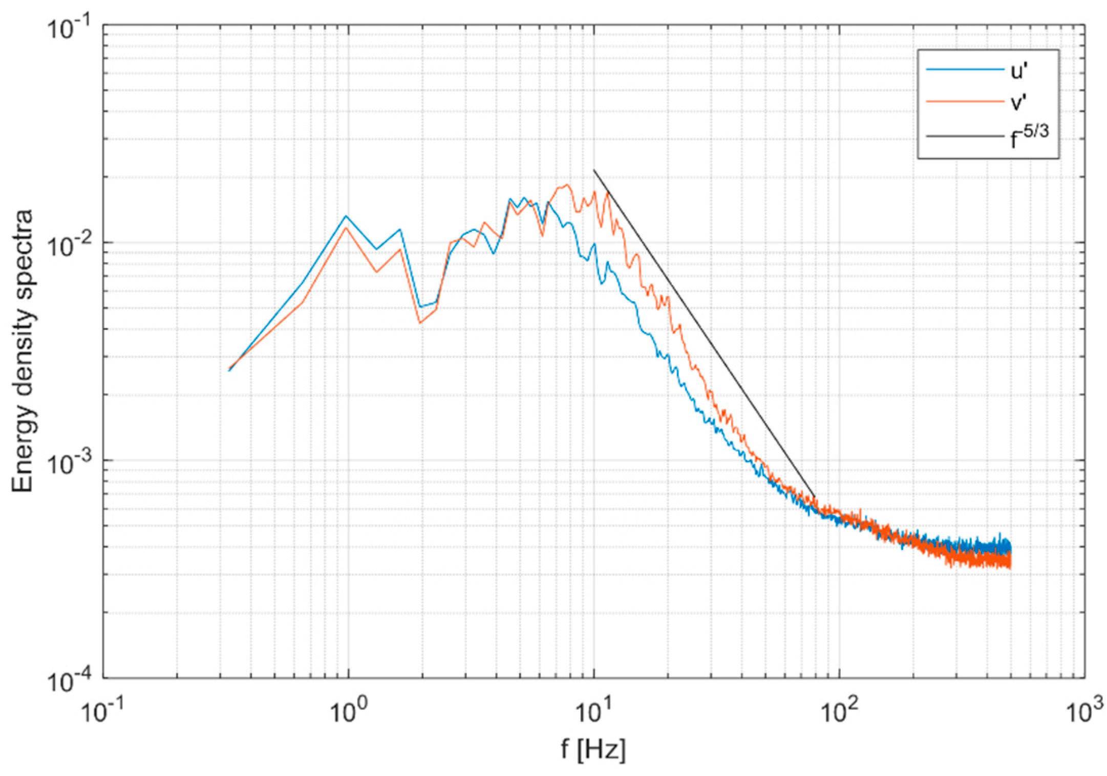
Further turbulent characteristics may be identified in the incoherent velocity data by consideration of the spectral energy content. Figure 18 presents the density energy spectra for both u and v components of the decomposed incoherent velocity dataset. In the figure, a line representing the −5/3 law is plotted, showing that the inertial range exhibits expected behavior up to 100 Hz, with the higher frequency content expected to be attributed to experimental error and noise.

This may be directly compared to the spectra obtained from the coherent velocity fields, presented in Figure 19. The behavior of this velocity data does not fit with the spectra expected for turbulent content. Furthermore, the peak at approximately 2 Hz is maintained from the original dataset, presented earlier in Figure 5. To aid interpretation of the presented spectra, the five-thirds law is plotted as a dashed line to contextualise the gradient.

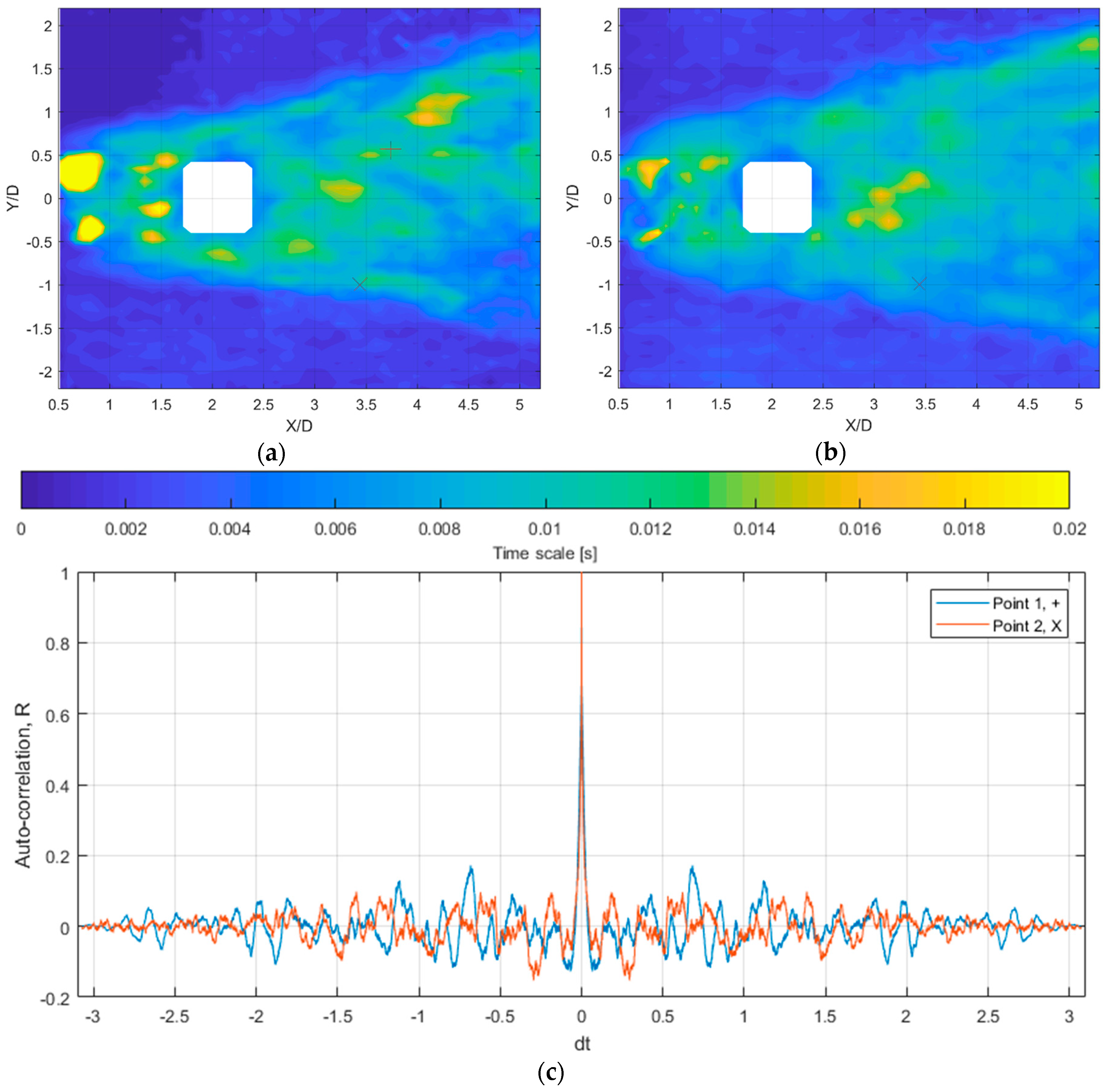
In a similar fashion to the length scales discussed, it is possible to use the time resolved point-based information to calculate the integral time scales associated with the flow. Figure 20a,b present the integral time scales associated with the decomposed turbulent fields for u-component and v-component respectively. It can be seen that the calculated values within the wake region are comparable for both components, indicating significant isotropy.

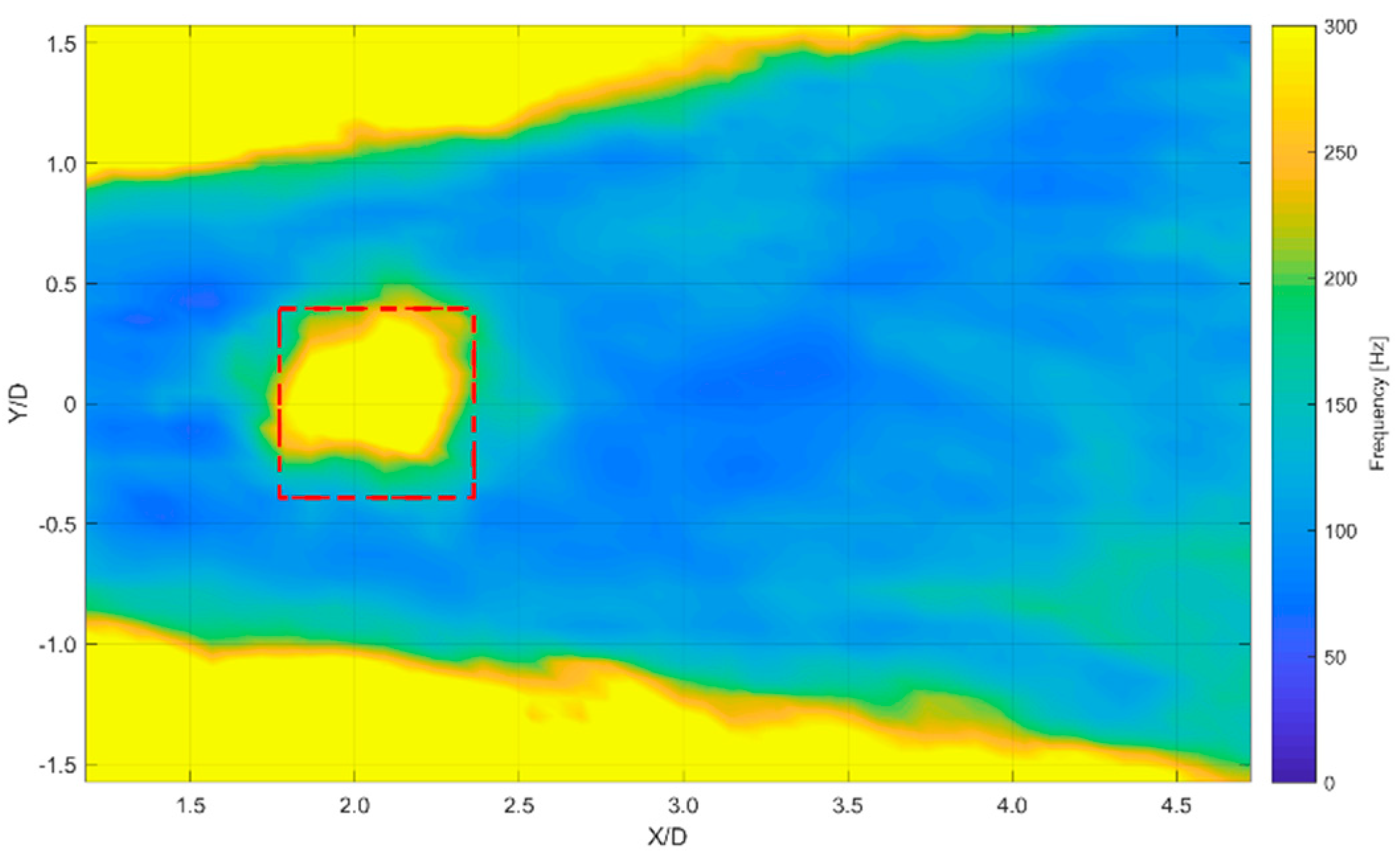
Outside of the wake area, much lower values are calculated, of the order 0.001 and below; this appears to be a consequence of the flow in this area having negligible turbulence, as shown in Figure 4. Therefore, once the coherent content is removed, the calculation is not reliable in this area due to low auto-correlation. The average time scale may be obtained from the two distributions in Figure 20, allowing the equivalent frequencies to be calculated, presented in Figure 21. The upper limit for colour scale is chosen to cover the range of frequencies within the wake region (high RMS). It is evident that the majority of the content in the wake region is below 150 Hz, suggesting that the tail in Figure 18 and Figure 19 is associated with experimental noise, evident when considering the freestream region. This noise may be filtered by an appropriate method such as low-pass frequency filter, as required.

Evident in the wake region is an anomalous area which has been omitted from analysis throughout the paper and masked in all figures except Figure 2a. An optical aberration, as mentioned in the method section was responsible for this. In all but the time and length scale analysis, the data in this region has looked contiguous and credible within the rest of the field (up to and including Figure 15). However, the frequency and lengthscale analysis identified that there is a strong noise content to the velocity signal in this region, hence it has not been included within the analysis. This is highlighted here to show how only considering first and second order statistical analysis of data may not always indicate when there could be underlying quality issues with the measured data.

4. Conclusions

In this paper, a methodology for the separation of coherent motions and turbulent fluctuations from spatially distributed experimentally obtained datasets is suggested and described. The methodology uses the well-established proper orthogonal decomposition (POD) technique to derive spatial eigenmodes associated with the flow which are then cross-correlated between two independent datasets, introducing a new metric, R. This value presents the correlation matrix between spatial modes of the independent datasets, allowing definition of those which relate to coherent motions, through high correlation, and those related to incoherent motions, through low correlation.

The methodology has been demonstrated on the commonly studied condition, a cylinder in cross-flow, revealing reported phenomena in addition to information that would otherwise not be possible to extract. Distributions of turbulent length and time scales reveal the characterisation of the structures within the wake region that would overwise be distorted by including coherent fluctuations within the analysis, for example, considerably overestimating the integral lengthscale.

References

1. Ölçmen, S.; Ashford, M.; Schinestsky, P.; Drabo, M. Comparative Analysis of Velocity Decomposition Methods for Internal Combustion Engines. Open J. Fluid Dyn. 2012, 2, 70–90. [Google Scholar] [CrossRef] [Green Version]
2. Stone, R. Introduction to Internal Combustion Engines, 4th ed.; Palgrave Mscmillan: Basingstoke, UK, 2012; ISBN1 9780230576636 (hbk.). ISBN2 023057663X. [Google Scholar]
3. Butcher, D.S.A. Influence of Asymmetric Valve Timing Strategy on In-Cylinder Flow of the Internal Combustion Engine; Loughborough University: Loughborough, UK, 2016. [Google Scholar]
4. Adrian, R.J.; Christensen, K.T.; Liu, Z.-C. Analysis and interpretation of instantaneous turbulent velocity fields. Exp. Fluids 2000, 29, 275–290. [Google Scholar] [CrossRef]
5. Lumley, J.L. The Structure of Inhomogeneous Turbulent Flows. In Atmospheric Turbulence and Wave Propagation; Publishing House Nauka: Moscow, Russia, 1967; pp. 166–178. [Google Scholar]
6. Chatterjee, A. An introduction to the proper orthogonal decomposition. Curr. Sci. 2000, 78, 808–817. [Google Scholar] [CrossRef]
7. Holmes, P.; Lumley, J.L.; Berkooz, G. Turbulence, Coherent Structures, Dynamical Systems and Symmetry; Cambridge University Press: Cambridge, UK, 1996. [Google Scholar]
8. Sirovich, L. Turbulence and Dynamics of Coherent Structues. Part I: Coherent Structures. Q. Appl. Math. 1987, 45, 561–571. [Google Scholar] [CrossRef]
9. Brindise, M.C.; Vlachos, P.P. Proper orthogonal decomposition truncation method for data denoising and order reduction. Exp. Fluids 2017, 58, 28. [Google Scholar] [CrossRef]
10. Butcher, D.; Spencer, A.; Chen, R. Influence of asymmetric valve strategy on large-scale and turbulent in-cylinder flows. Int. J. Engine Res. 2018, 19, 631–642. [Google Scholar] [CrossRef]
11. Epps, B.P.; Techet, A.H. An error threshold criterion for singular value decomposition modes extracted from PIV data. Exp. Fluids 2010, 48, 355–367. [Google Scholar] [CrossRef]
12. Raiola, M.; Discetti, S.; Ianiro, A. On PIV random error minimization with optimal POD-based low-order reconstruction. Exp. Fluids 2015, 56. [Google Scholar] [CrossRef]
13. Doosttalab, A.; Dharmarathne, S.; Bocanegra Evans, H.; Hamed, A.M.; Gorumlu, S.; Aksak, B.; Chamorro, L.P.; Tutkun, M.; Castillo, L. Flow modulation by a mushroom-like coating around the separation region of a wind-turbine airfoil section. J. Renew. Sustain. Energy 2018, 10. [Google Scholar] [CrossRef]
14. Norberg, C.; Sunden, B. Turbulence and reynolds number effects on the flow and fluid forces on a single cylinder in cross flow. J. Fluids Struct. 1987, 1, 337–357. [Google Scholar] [CrossRef]
15. Park, J.; Choi, H. Numerical solutions of flow past a circular cylinder at reynolds numbers up to 160. KSME Int. J. 1998, 12, 1200–1205. [Google Scholar] [CrossRef]
16. Behrouzi, P.; McGuirk, J. Experimental data for CFD validation of impinging jets in cross-flow with application to ASTOVL flow problems. In Proceedings of the AGARD Conference Proceedings 534, Computational and Experimental Assessment of Jets in Cross-Flow, Winchester, UK, 19–22 April 1993. [Google Scholar]
17. Perrin, R.; Cid, E.; Cazin, S.; Sevrain, A.; Braza, M.; Moradei, F.; Harran, G. Phase-averaged measurements of the turbulence properties in the near wake of a circular cylinder at high Reynolds number by 2C-PIV and 3C-PIV. Exp. Fluids 2007, 42, 93–109. [Google Scholar] [CrossRef]
18. Perrin, R.; Braza, M.; Cid, E.; Cazin, S.; Barthet, A.; Sevrain, A.; Mockett, C.; Thiele, F. Obtaining phase averaged turbulence properties in the near wake of a circular cylinder at high Reynolds number using POD. Exp. Fluids 2007, 43, 341–355. [Google Scholar] [CrossRef]
Figure 1. Schematic of LU horizontal water flow tunnel. Indicative measurement plane represented with horizontal green line, downstream of test piece.
Fluids 04 00134 g001
Figure 2. Experimentally obtained flow fields. (a) Instantaneous vector field, (b) Ensemble average stream lines. Colour represents velocity magnitude, normalized by free-stream velocity, U0.
Fluids 04 00134 g002
Figure 3. Velocity profiles (y-direction) at selected points downstream. (a) x-component, (b) y-component.
Fluids 04 00134 g003
Figure 4. Velocity RMS distribution for full dataset.
Fluids 04 00134 g004
Figure 5. Field averaged spectral energy density for measured velocity components.
Fluids 04 00134 g005
Figure 6. Demonstration of velocity convergence with number of samples. (a) PDF of error in u velocity, ε u for 1536 snapshots; (b) Trend of standard deviation of error, σ with increasing samples calculated from PDFs; (c) Field average velocity RMS convergence.
Fluids 04 00134 g006
Figure 7. Comparison of energy fraction for each proper-orthogonal-decomposition (POD) mode of Set A and B. Curtailed at mode 25 for clarity.
Fluids 04 00134 g007
Figure 8. POD spatial modes: (a) SA = 1, (b) SB = 1, (c) SA = 2, (d) SB = 2, (e) SA = 3, (f) SB = 3. Color scale represents magnitude and is normalized to a common factor across all subfigures.
Fluids 04 00134 g008aFluids 04 00134 g008b
Figure 9. POD temporal coefficient analysis for early modes. (a) First, a1 and second, a2 temporal coefficients; (b) Spectral energy content for the first three sets of temporal modes.
Fluids 04 00134 g009
Figure 10. POD spatial modes for higher order: (a) SA = 30, (b) SB = 30. Color scale represents magnitude and is normalized to a common factor.
Fluids 04 00134 g010
Figure 11. Absolute cross-correlation of POD spatial modes from set A and B. Curtailed at 31 for clarity.
Fluids 04 00134 g011
Figure 12. Maximum absolute correlation for each POD spatial mode (curtailed at mode 50). Smoothed data is used to produce trend. A cut-off at 60% correlation is indicated.
Fluids 04 00134 g012
Figure 13. Example of a decomposed instantaneous vector field. (a) Coherent part; (b) incoherent part (vectors shown white for clarity); (c) raw velocity field. Colour scale represents velocity magnitude normalized with free-stream velocity, U0.
Fluids 04 00134 g013
Figure 14. Diagrammatic overview of methodology.
Fluids 04 00134 g014
Figure 15. Comparison of fluctuating flow fields for an example flow field. (a) Original flow field; (b) All fluctuations (Reynolds decomposition); (c) Coherent part; (d) incoherent part. Colour scale represents velocity magnitude (common scale).
Fluids 04 00134 g015
Figure 16. Integral length scales associated with (a,b) coherent fields, 1L11 and 2L22 respectively; (c,d) turbulent fields, 1L11 and 2L22 respectively. Note colour scale changes between subfigures. Parentheses values in (c) and (d) are mm.
Fluids 04 00134 g016
Figure 17. Probability density functions (pdf) of velocity components. (a) Original data; (b) all fluctuations—Reynolds decomposed; (c) coherent part; (d) turbulent part.
Fluids 04 00134 g017
Figure 18. Spectral energy density for turbulent fluctuations, u’. Five-thirds law plotted for reference.
Fluids 04 00134 g018
Figure 19. Spectral energy density for coherent fluctuation velocities, u*. Five-thirds law plotted for reference.
Fluids 04 00134 g019
Figure 20. Integral time scale distributions associated with turbulent parts. (a) uu; (b) vv; (c) Auto-correlation function, uu about two example points, locations indicated in (a) and (b).
Fluids 04 00134 g020
Figure 21. Spatial distribution of frequency content associated with integral time scales in turbulent field ( 1 / τ ) , scaled appropriately to the wake region only.
Fluids 04 00134 g021