1. Introduction
Oceanic rogue waves have attracted significant attention in recent years, becoming a well established subject of studies in the last two decades after a long period in which they were rather regarded as part of the maritime folklore and sailors’ legends. Reminiscence of their legendary past is evident in the many names they have: rogue waves are also called freak, giant, anomalous, extreme, killing or monster waves. These are exceptionally high waves, substantially higher and steeper than those expected for a given sea state. Their existence has been now confirmed by a variety of observations. Their appearance in scientific literature probably dates back to 1964 when Draper presented a first description of the phenomenon in [
1]. While in [
2] one finds an initial discussion of rogues waves off the southeast African coast, in the Agulhas current, it is essentially in the last decades, thanks also to more reliable wave recordings as wave measurements from oil platforms, that they received wider attention from the scientific community as well as from the shipping and offshore industry [
3,
4,
5,
6]. Probably the best known reliable recording of a rogue wave is the so-called New Year wave, or Draupner wave [
7,
8], recorded at the Draupner platform in the North Sea off the coast of Norway on 1 January 1995. The Draupner wave was confirmed by damage to equipment on the platform deck, so it could not be classed as a measurement error, as it happened often with previous recordings. Even though the existence of rogue waves has been confirmed by various observations, their origin remains a debated subject (see, e.g., [
8,
9,
10]). In this respect, contributions came also from lab experiments as rogue waves have been observed in tank to test the NLS equation as model of rogue wave generation by modulation instability of a long regular wave train [
11,
12,
13,
14]. Rogue waves have also been observed in tanks under controlled wind generation [
15,
16]. It should also be mentioned that it has been recently recognised that, in the near future, the significance of severe sea state conditions may even grow in some ocean regions because of the expected increase in the frequency and severity of extreme weather events associated with global warming [
17].
The initial stage of instability of a quasi-monochromatic plane wave is characterised by the exponential growth of a small localised bump of the monochromatic envelope. The short time evolution of this initial perturbation depends on the eigenmodes of the linearised NLS equation around this monochromatic wave. Our purpose here is to infer from these eigenmodes the instability bands and the corresponding rate of growth of a small perturbation. The important question of the long time nonlinear stage of the evolution is out of the scope of the present work (see, e.g., [
18,
19]). In the past decades, the main focus has been directed on the generation of rogue waves and on the conditions under which such waves are more likely to occur. This work has revealed the existence of similar extreme phenomena in other physical contexts, such as nonlinear optics and lasers [
20], atmosphere [
21], plasma physics [
22], and matter waves (Bose–Einstein condensate) [
23,
24]. These investigations have given further impulse, and the interest in rogue waves is today a well motivated multidisciplinary research area on its own (see also [
25,
26]).
Because of the common acceptance of the crucial role that nonlinearity plays in ocean wave dynamics, especially so in rogue wave formation, and because of the computational burden of solving the full nonlinear equations describing the sea state numerically, much of the work done on rogue waves has been carried out using approximate models. An important class of such models, which has been widely used in rogue wave research, is that of Nonlinear Schrödinger (NLS) equations. In oceanography, NLS-type equations can be derived from the full Euler equations by assuming that waves are weakly nonlinear, with small wave steepness, and narrow banded. The simplest NLS equation
accounts for quadratic dispersion and cubic nonlinearity of the slowly varying amplitude of just one quasi-monochromatic wave (for a simple derivation by multi-scale perturbation method, see, for instance, [
27]). Indeed, this equation plays the role of a universal model [
28] as it emerges by wisely approximating almost any conservative wave dynamics. This accounts for its ubiquity in physical applications, wherever the conditions of weak dispersion and nonlinearity, and of narrow band, are met. By the same token, the way the NLS equation is derived also explains its integrable character since it also approximates known wave equations such as the Korteweg–de Vries equation for shallow water waves, which is well-known to be integrable [
29]. Thus, whenever the wave motion can be considered in a one-dimensional space, the NLS equation is a universal
and integrable model with powerful implications for both its physical relevance and mathematical properties. In this respect, the NLS equation has deserved further special interest as it proves to yield, for focusing interaction, a simple description of the instability of a regular wave train, a phenomenon first observed by Talanov [
30] in optics and by Benjamin and Feir [
31] in a water tank. Such instability is responsible for breaking a plane wave into irregular motion and eventually for generation of novel wave patterns such as rogue waves [
19,
25] (see also, e.g., [
32]). Today, for the scalar NLS equation, the focusing nonlinear regime is well recognised to be a prerequisite for the emergence of rogue waves. On the contrary, the defocusing regime of the NLS equation does not allow for rogue wave solutions, even of dark nature. In fact, the linear stability analysis of the background continuous wave solution in focusing and defocusing regimes is sufficient to make such distinction [
33]. In addition to its proven validity, laboratory observations show that the accuracy of the NLS equation is even higher than expected [
11,
34].
The research area on rogue waves goes well beyond water waves dynamics and extends itself to quite a number of different fields. We deem it worth mentioning that some of them, although not quite ocean physics, have recently received a new impulse from the novel extension of soliton theory to nonlocal equations, namely to models with parity-time symmetry, and time symmetry. In particular, these extended models are, among many others, the nonlocal NLS, coupled NLS and Davey–Stewartson equations [
35,
36,
37].
Since numerous physical phenomena require modelling waves with two or more components to account for different modes, frequencies, or polarisations, coupled-wave systems have recently attracted the interest of the research community. In such systems, however, the situation is much richer, and it has been shown in [
38,
39] that rogue wave solutions can exist also in the defocussing and mixed regimes [
38]. Again, by applying the perturbation method of multiple scale, as in the derivation of the NLS equation, to the envelopes of two quasi-monochromatic waves, and by adding an appropriate weak resonance condition, one arrives at a system of two coupled NLS equations (for such derivation in the description of crossing sea waves, see [
40,
41,
42]). The difference with respect to the single NLS equation is that such system, although it still features quadratic dispersion and cubic nonlinearity, is less universal as it has a larger number of coupling constants, and it is generically non-integrable, although with few important exceptions. In this paper, we take advantage of the existence of integrable versions [
43] of a system of two coupled NLS equations to explore the connection between the instability properties of the plane wave solution and the existence and features of rogue wave solutions. Thus, in
Section 2, we first introduce the definition of the
stability spectrum via the construction of the eigenmodes of the linearised wave equations, and then we give a complete classification of such spectra in the parameter space, namely for different values of coupling constants and amplitudes. Relating then the geometrical properties of the spectrum to rogue waves, in
Section 3, we classify also the set of rogue wave solutions, and give their expression via the standard Darboux–Dressing technique [
38,
44,
45]. By numerical computations, we look into few properties of these wave solutions, such as their amplitude height for the sake of comparing them with the analogue Peregrine solution of the NLS equation. According to their relation to spectra, examples of each type of rogue wave solutions are graphically shown.
Section 4 is devoted to conclusions.
2. CNLS: Spectra and Stability
Since a main ingredient in the occurrence of rogue waves has been recognised [
38,
39] to be the instability of their background state, our main focus here is on the linear stability of continuous waves (CW). Moreover, it has been also realised [
46] that the stability of two CWs, which are weakly at resonance, features a richer phenomenology with respect to that associated to just one plane wave [
47]. Thus, we devote this section to collect and emphasise such novel features by discussing the stability of CW solutions of the following two coupled nonlinear Schrödinger (CNLS) equations
Here, and in the following, a subscripted continuous variable, such as
x and
t, which are the slow space-time coordinates, stands for partial differentiation with respect to that variable. The two dependent variables
,
, are the (rescaled) complex envelope amplitudes of two quasi-monochromatic waves that are weakly resonant and propagate with self- and cross-interactions. The interactions are modelled by cubic terms with real coupling constants
and
. Coupled equations of this kind, perhaps with different interaction terms and dispersion coefficients, may be derived by multi-scale analysis in several contexts, mainly in optical fibres [
48] but also in multi-component Bose–Einstein condensates [
23], and in few instances of surface gravity waves in deep water [
41]. A limitation to their applicability to water wave propagation comes from the weak resonance condition which requires that the two carrier waves have nearly the same group velocity, which, in turn, is a condition on the carrier waves linear dispersion relation. Our preference for the system in Equation (
1) is motivated by its peculiar, and exceptional, property of being integrable for any choice of
and
[
43]. In fact, as shown below, the integrability property does allow one to use powerful, and rather direct, both analytical and numerical, methods to investigate the linear stability of a given solution
,
of the CNLS equations in Equation (
1). Moreover, even if the model in Equation (
1) is not exactly the one of interest, it is sufficiently close to it that we believe investigating this integrable model is worth doing as the resulting dynamics may serve as reference guide to deal with similar, but non-integrable, equations.
With no loss of generality, we give the coupling constants the rescaled values
,
. Thus, the system in Equation (
1) describes three different physical settings: the defocusing Manakov model for
, the focusing Manakov model for
and the mixed case
. This system is therefore a natural integrable vector generalisation of the NLS scalar equation which is obtained from Equation (
1) by merely setting
. In our present setting, its integrality stems from the existence of its associated Lax pair of matrix linear ordinary differential equations
which are compatible with each other if the following equation
is satisfied. Both matrix coefficients
and
are
, and have the simple polynomial dependence on the complex
spectral variable
where
and
Hereafter, the upper scripted asterisk means complex conjugation and the squared bracket
is the usual commutator
. The choice in Equation (
4) of the matrices
and
implies that the compatibility condition in Equation (
3) is equivalent to the CNLS system in Equation (
1). As is well known (see, e.g., [
49]), the
-dependence of the Lax pair in Equation (
2), together with the assumption that the wave fields
and
vanish sufficiently fast as
, is the departure point of the spectral (alias inverse scattering) transform method, which is the nonlinear analogue of the Fourier transform (see [
50] and the introductory lecture [
51]). The mathematical setting required by the application of the spectral transform is rather cumbersome, and becomes even more so if the boundary values of the solution
,
do not vanish as
, as ideally happens when dealing with CW solutions. However, since our aim here is confined to establishing only the linear stability of a given solution of the CNLS system, we take a simpler route. As is standard, the investigation of the linear stability of any known solution
,
of the CNLS equations in Equation (
1) starts with the linear equations
for the unknown functions
and
. This system originates from the assumption that
,
is an approximate solution of the CNLS system in Equation (
1), provided
,
is a sufficiently small solution of Equation (
7). Hereafter, we consider only perturbations
,
whose initial data are assumed to be
localised (and bounded) in
x. Proving that the solution
,
be linearly stable requires showing that the initially small data
,
remain small at any time
t. A standard way to face this problem is to construct a (complete) set of solutions
,
of the linear Equation (
7),
These solutions, the eigenmodes, depend on the spectral parameter
with the implication that the solution of Equation (
7) can be formally represented as the linear combination
As shown below in the case of CWs, the expression of these eigenfunctions is sufficient to prove stability while there is no need to actually compute the integral in Equation (
9). Indeed, the knowledge of such set of solutions, i.e., the eigenmodes, allows one to compute: (i) the
stability spectrum , which is the appropriate subset of the complex
-plane over which the integral (
9) runs; (ii) the dispersion relation associated to the linearised Equation (
7); and, quite importantly, (iii) the gain, namely the function of
that characterises the temporal growth of each unstable eigenmode (see below).
The construction of eigenmodes is made rather simple and direct by the following procedure. Suppose
,
is a known given solution of the CNLS equations, then the first step is to compute a corresponding fundamental
matrix solution
,
, of the Lax pair in Equation (
2). The second step merely requires computing the matrix
. A solution
,
of the linearised Equation (
8) takes the explicit expression of the
and
entries of the following matrix
FHere, the matrix
, apart from some algebraic condition, is arbitrary and
x- and
t-independent. We omit detailing its explicit expression since it is not relevant to our present purposes. We note however that this computational way to construct eigenmodes is quite general, as it remains valid for a very large class of integrable systems. It has been used in several contexts and in different formulations, in particular in soliton perturbation theory, where these eigenmodes have been termed
squared eigenfunctions [
52,
53]. A general derivation of Equation (
10) from the Lax pair is given in [
46], with no need to cope with the burden of the direct and inverse spectral problem techniques.
We now follow the way outlined above to investigate the linear stability of the continuous wave solution
of the CNLS equations in Equation (
1). Here, the real parameter
p,
is given in terms of the coupling constants and of the amplitudes
and
that, with no loss of generality, are real and non-negative. The parameter
q, which has a relevant role in the following analysis, measures the half-difference of the wave numbers of the two continuous wave components in Equation (
11). In this respect, one should keep this parameter in mind, as it makes the stability properties of the continuous wave solution in Equation (
11) of the CNLS system considerably different from those due to Benjamin–Feir instability described by the single NLS equation. With no loss of generality, we have chosen to consider here the two CW components in Equation (
11) as counter-propagating. According to the general scheme, the first step requires constructing the matrix solution
of the Lax pair in Equation (
2). This is given by the expression
where the
x- and
t-independent matrices
W and
Z are found to be
with the property that they commute,
, consistently with the compatibility condition in Equation (
3). We consider here the eigenvalues
and
,
, of
and
, respectively, as simple, as indeed they are for generic values of
. Next, we construct the matrix
via its definition in Equation (
10), which, because of the explicit expression in Equation (13), reads
After some algebraic manipulation of this matrix expression in Equation (
16), and by taking into account Equation (
10), one ends up with the following equivalent way to express the eigenmode components
,
where we have introduced the
x- and
t-independent coefficients
and
that depend only on
. In addition, the coefficients
are
x- and
t-independent and are related to the matrix
which appears in Equation (
16). The advantage of Equation (
17) is to explicitly show the
x- and
t-dependence of the eigenfunctions
and
, see Equation (
10), through the six exponentials
. Moreover,
and
are solutions of linearised Equation (
8) for any choice of the functions
of the spectral variable. On the other hand, the requirement that the solution of Equation (
9) be localised in the variable
x implies few necessary conditions on the functions
. The further condition that the solution
be bounded in
x at any fixed time
t imposes integrating with respect to the variable
, see Equation (
9), over the spectrum
, that is an appropriate piece-wise continuous curve of the complex
-plane:
To define this spectrum
, we have to first introduce the three “wave-numbers”, see Equation (
17),
through the eigenvalues
of the matrix in Equation (
14) as complex functions of the spectral variable
. These are the differences of the three eigenvalues of the matrix
in Equation (
14). They appear in the eigenmodes in Equation (
17) with both signs and evidently satisfy the condition
. It should be also noted that the labelling by the index
j of the eigenvalues
, and therefore of the
s, is arbitrary and it does not imply any order. Then,
, namely the spectrum which is relevant to our present analysis, can be defined as follows:
Definition 1. The stability spectrum is the subset of values of the spectral variable λ such that at least one of the three wave-numbers , , see Equation (19), be real. The computation of the spectrum, as a piecewise algebraic curve in the complex
-plane, starts with this definition and requires a lengthy analysis which is detailed in [
54]. Two general features of
are the following: (1) The real axis of the
-plane always belongs to
, possibly with gaps, namely with finite forbidden intervals. This is the real part of the spectrum where the eigenmodes are stable. (2) A non-real component of the spectrum, which is symmetric with respect to the real axis, may occur for
. When
belongs to this part, the corresponding eigenmodes are unstable.
These features are present also in the well known spectrum associated to the scalar NLS equation to which our present formulation reduces as one of the two waves is not present, e.g.,
. In this case, the spectrum is extremely simple and can be calculated explicitly. In our present notation, with
,
, one finds [
47] two types of spectra. One for
(defocusing case): the spectrum has only the real part,
, which is the real axis with one gap,
, where the wave numbers are
,
,
. As for the second type for
(focusing case), the real part of the spectrum is the entire real axis,
, while its complex part, with
, presents itself as a branch, i.e., the finite interval
on the imaginary axis. Importantly, on this complex component of the spectrum, only the wave number
is real, and the other two wave numbers
,
are not real. On this part of the spectrum, eigenmodes are unstable since their amplitude grows exponentially with time. Although the modulational stability/instability, as modelled by the NLS equation in the defocusing/focusing regime, is very much known, our sketch of it given above is meant to emphasise the many differences between the NLS case and the stability/instability properties of the CNLS. In particular, we compare their spectra together with their physical implications.
Let us discuss now the spectra associated to the coupled CW solutions in Equation (
11). Now, it obviously happens that, with respect to the scalar NLS equation, more parameters come into play. In addition to the wavenumber mismatch
q between the two background waves in Equation (
11), the two parameters
in Equation (
12), and
are conveniently replacing the coupling constants
and
and the amplitudes
and
. As for the parameter
q, it is worth observing that the case
can be explicitly treated [
46], and it leads to defocusing and focusing effects, which are similar to those associated to the NLS equation. Thus, we consider
only non-vanishing values of
q, say
, which could also be rescaled to the value
. We also observe that one may consider, with no loss of generality (see [
46]), only non-negative values of
r and positive values of
q. Thus, the parameter space we explore in the following analysis is the half
plane with
. To each point of this parameter space there corresponds a spectrum
, and our goal is to classify all types of spectra in this space.
We start with few observations of general validity, whose proof is given in [
54]. In addition to the two reality properties of the stability spectrum mentioned above, we note that the three wave numbers
can all be real if and only if
is real. If
is not real,
only one of the wave numbers
,
, or
can be real. Moreover, our analysis shows that spectra are specifically classified according to whether they possess the following geometrical features:
gaps on the real axis, and, in the non-real part, algebraic curves which may be open, termed
branches, or closed, termed
loops. Regarding gaps and branches, the following result holds true [
46]: if
G is the number of gaps and
B is the number of branches, then, for any generic value of the parameters
the spectrum satisfies the condition
As for loops
L, we note that for any generic value of the parameters
the spectrum
may have either one loop or none. Our geometric classification of spectra can be summarised by the following statement: if all spectra are characterised by their number of gaps, branches and loops, then, for any generic value of the parameters
, the spectrum can be only one out of the following five different types of spectra:
where the notation
stands for
n components of type
X, with
X being
G,
B, or
L [
46].
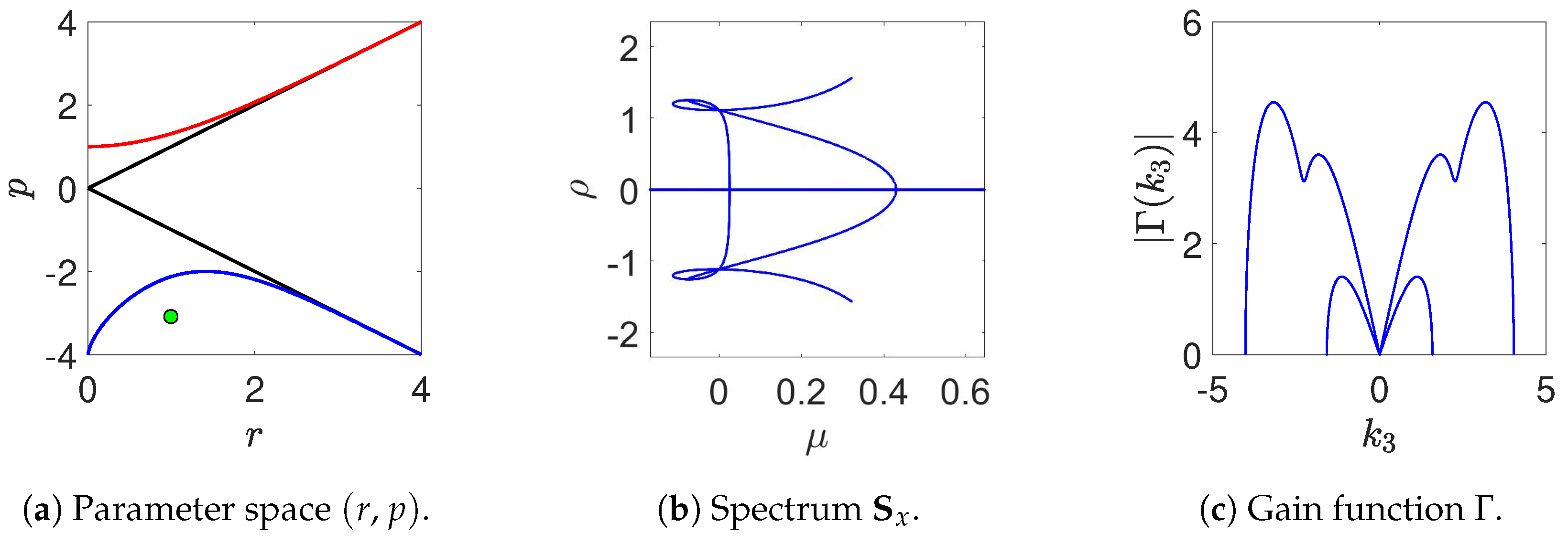
The parameter space is thus divided into regions, in each of which the spectrum remains of the same type by varying the parameters
. The spectrum changes by crossing the region boundary curves. These boundaries are explicitly known threshold curves (details can be found in [
46,
54]). This classification, viewed as regions of the
half-plane, together with their boundary curves, is shown in
Figure 1. In this figure, the defocusing case
corresponds to
, the focusing one
to
and the mixed case
to
.
In
Figure 2, we plot examples of the five types of spectra
as in Equation (
22). These are shown in the plane
where the real variables
and
are the real and imaginary parts, respectively, of the complex spectral variable
.
The limit case
is discussed and displayed in [
54].
As already noticed, to the purpose of establishing the stability properties of the continuous wave solution of Equation (
11), we do not need to compute the integral representation in Equation (
18) of the solutions
of Equation (
7). Indeed, it is sufficient to compute the “eigenfrequecies”, whose definition
is suggested by the exponentials which appear in Equation (
17). They are real on the real part of the spectrum, e.g., for any
. On the contrary, if
belongs to the non-real component of the spectrum, only one wavenumber, e.g.,
, is real while its corresponding frequency is complex
This happens if
lies on a branch or on a loop. The imaginary part
of
is the
gain (or growth) function, which is different from zero only on branches and loops, namely on a finite instability band of wave numbers. In this respect, we note that the instability band that is associated to a branch differs from that associated to a loop. This difference is of practical interest since in the first case (branch) the band is around
—this instability being commonly known as
baseband instability (see, e.g.,
Figure 3) as it involves very long wavelengths. This is similar to the Benjamin–Feir instability described by the (focussing) NLS equation. The one associated instead to a loop is known as
passband instability (see, e.g.,
Figure 4), which does not include vanishingly small wave numbers [
55,
56]. This kind of instability does not occur for one single plane wave. Indeed, as predicted by the NLS equation, loops are not present in the single CW instability spectrum. Moreover, for two resonating CWs, branches and loops may be both present in the spectrum (see Equation (
22)), and therefore two different instability bands may partially overlap and lead to a rather complicate overall gain function (see, e.g.,
Figure 5 and
Figure 6).
3. CNLS: Rogue Waves and Spectra
In the previous section, we construct and display the stability spectrum
of two weakly resonant plane waves. This is definitely more complicated than the one associated to just one plane wave. Moreover, the spectrum depends on parameters that cannot be got rid of by rescaling, such as the ratio
of the CW amplitudes, or which cannot be set to vanish by changing the frame of reference, such as the mismatch
q of the wave numbers of the background waves. This richness is evident in a number of predictions of new phenomena associated to the CNLS model. For instance, as already observed [
38,
39] and in contrast with the instability predicted by NLS equation, new kinds of instabilities occur in defocusing regimes. As pointed out in the extensive literature [
57], instabilities lead to generation of nonlinear wave patterns. Although the generation mechanism is out of the scope of the present work, we aim here to investigate the existence, construction and properties of rogue wave (RW) solutions by taking advantage of our spectral approach to linear stability. In particular, by taking into account the stability spectra described in the previous section, we provide an exhaustive classification of RW solutions of the CNLS equations in Equation (
1) together with their identification in the complex
-plane of the spectral variable.
Motivated by their well established relevance to several observations in oceans and in fibre optics, rogue waves have been investigated mainly as solutions of integrable models. The prototype wave profile pointed out by Peregrine [
58] attracted the attention of physicists since, among other reasons, it is not periodic and its amplitude is three times higher than that of the background. On their side, mathematicians found this bounded solution of interest for its rational, rather than exponential, dependence on the space-time variables [
38]. These special features of rogue wave profiles proved to be useful to searching for RWs in integrable model equations (see below and [
38]). Combining this requirement on the space-time dependence with the distribution over the spectrum
of wave numbers
of the eigenmodes of the linearised equation (see Equation (
7)), leads to a definite rule to find RW solutions. Indeed, the RW discrete eigenvalues, referred to hereafter as the
critical values in the complex plane of the spectral variable
, turn out to be the (strictly) complex solutions
of the equation
. This rule is the consequence of the following arguments. As follows from our analysis reported in the previous section, and better detailed in [
46,
54], only one of the three wave numbers
, e.g.,
, is real if
is complex (i.e., on branches and loops) or, if
is real, it lies at the end points of gaps. Moreover, the equation
has four solutions. They may come as pairs of real values that lie at the end points of gaps of the spectrum, or pairs of complex conjugate values at the extremes of branches. However, soliton solutions of the CNLS equations, whose corresponding discrete eigenvalue solve the equation
at the endpoints of a gap, are singular in
x; consequently, the acceptable solutions
have to be strictly off the real axis,
, and thus located at the complex conjugate extremes of branches of the spectrum. On the other hand, if
were non-vanishing, then the eigenmodes would be periodic (see Equations (
17) and (
19)) against the condition that the rogue wave solutions have rational (or semi-rational) dependence on
x. This establishes a one-to-one correspondence between branches and RWs. A very simple example of this rule is shown by the stability spectrum of the NLS equation: for this equation, there exist only two types of spectrum. If the interaction is defocusing, the spectrum is
type with no RW solution, while in the focusing case the spectrum is
type with the Peregrine soliton critical values
and
at the two extremes of the branch. Similarly, but in a far richer scenario, RW solutions of the coupled NLS equations correspond to eigenvalues
that lie at the two extreme points of each branch.
In the previous section, we point out that, for
, the spectrum
of the linearised equation around the CW solution of Equation (
11) changes in the plane of the parameters
in such a way that this plane gets divided in five regions (see
Figure 1). Within each region the spectrum is one of the five different types (Equation (
22)) with the consequence that also RW solutions can be divided into different types according to the fixed
point in the parameter space. The construction of the RW solution may go via the Darboux–Dressing technique [
38] which requires fixing the seed solution, namely the CW (Equation (
11)), and the particular
. The correspondence branch-RW discussed above readily implies that there cannot be any RW solution if the point
lie in the region where the spectrum is
. As shown in
Figure 1, this region is partly in the defocusing section
,
for
, and in the mixed section
,
if
. Note that all threshold curves have an explicit analytic expression; we refer the interested reader to [
46,
54] for details.
As for the remaining four type of spectra, two of them have one branch, while the other two have two branches. The computation of the critical value
, at a
generic point
in the appropriate spectral region (see
Figure 1) is obtained numerically as root of the following fourth-degree polynomial [
54]:
which has two real and two complex conjugated roots if the spectrum is of type
or
, and has two pairs of two complex conjugated roots if the spectrum is instead
or
. Non-generic limit values of
, which have an explicit expression, are mentioned below. Once the critical value
is known either numerically or analytically, the computation of the corresponding RW solution may proceed via the standard Darboux–Dressing method (or by other equivalent ways). Omitting details (which can be found in [
38]), the final expression of such solution takes the explicit form
The parameters
,
,
,
,
q, and
p, which appear in this expression, are defined in
Section 2. The functions
V,
, and
are the components of the vector
where the constants
c,
,
and
m are arbitrary complex parameters. Here, the
matrix
U is
x- and
t-independent and reads
while the velocity
g in Equation (
27) turns out to be
We note that the
x- and
t-dependence of the three-vector in Equation (
27) is both polynomial and exponential so that the RW profile turns out to be a mixture of rational and exponential functions for a generic choice of the free parameters. To complete the construction of the RW solution by Equation (
26), it remains to obtain the expression of the simple eigenvalue
and of the double eigenvalue
of the matrix in Equation (
14). However, since they are linked to each other by the trace relation
, we need to give only the expression
Moreover, the wave number
and frequency
, which appear in the expression of the vector in Equation (
27), are defined by Equations (
19) and (
23) and read
where we have made use of the matrix relation in Equation (
15).
Once all free parameters have been fixed and a critical value of the spectral variable has been computed, Equation (
26), obtained from the Darboux (or Darboux–Dressing) method, is the basic tool to plot rogue wave profiles and to explore their properties.
Figure 7,
Figure 8,
Figure 9,
Figure 10,
Figure 11,
Figure 12 and
Figure 13 show examples of RW solutions that are generic and each one attached to one of the four different types of spectra (see captions). It is worth pointing out that solutions are purely rational for the choice
and
; and are generally rational-exponential otherwise. We also note that in each of these figures we choose to fix the numerical values of the parameters
r and
p and to consequently obtain the values of the wave amplitudes
and
through the definitions in Equations (
20) and (
12); this is why the values of the amplitudes may look rather odd. For each solution, one could ask for which choice of the arbitrary constants
c,
and
one would obtain maximal amplitudes. This question can be answered using a Nelder–Mead Simplex Method [
59], as implemented in the
fminsearch MATLAB_R2018a routine, and an example is given in
Figure 11. The corresponding purely rational solution for the same choice of
r,
p and
as in
Figure 11 is shown in
Figure 10.
For the last case, namely
, we consider two RW solutions, corresponding to the two branches (see
Figure 12 and
Figure 13); numerical evidence suggests that the RW corresponding to the brach associated to
with the larger imaginary part has a larger amplitude, as one would expect by inspecting the gain function.
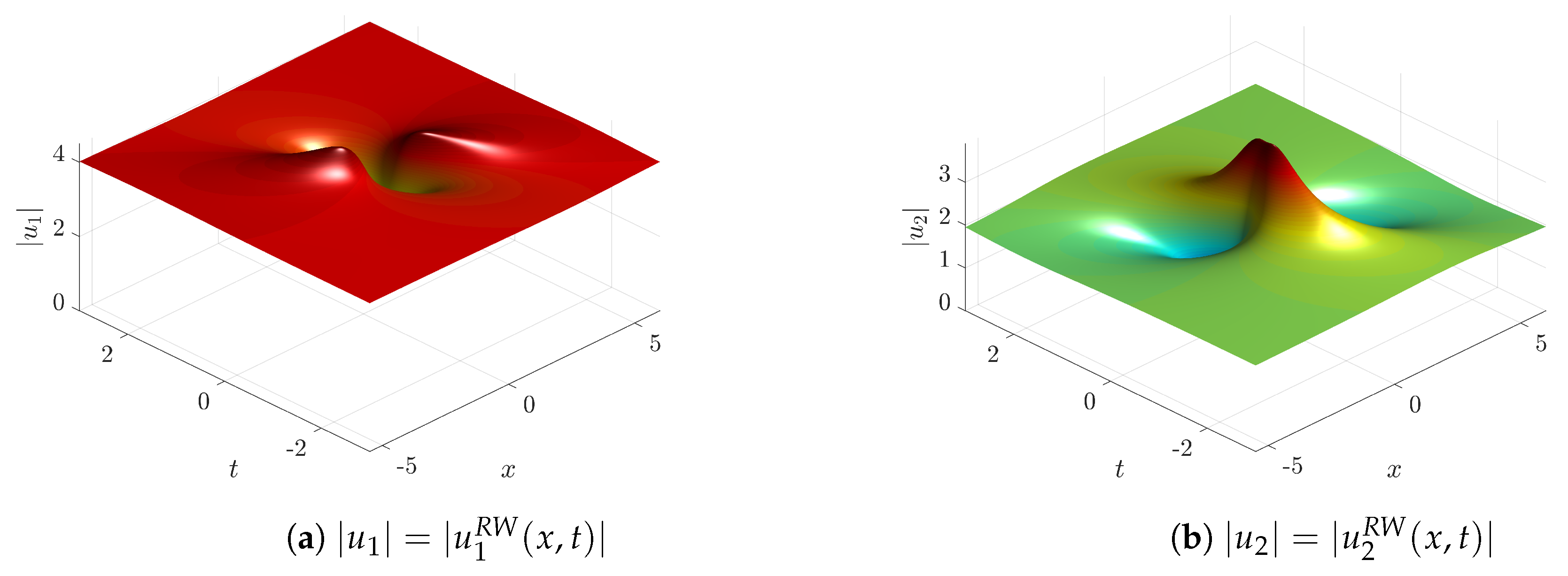
As for non-generic choices of the parameters and q such as or , we briefly mention below RW solutions that enjoy an explicit analytical expression together with new physical features, such as amplitude bumps (depressions), which are higher (lower) than that of the Peregrine soliton.
The first example of non-generic solutions is that of RWs over two co-propagating coupled background waves, e.g., the plane–wave solution of Equation (
11) with
(see
Figure 14). The following solution is the analogue of the Peregrine rogue wave in the present case of two coupled NLS equations [
38,
60]. Indeed, as for the NLS equation, the parameters for this solution are
and, as for the focusing interaction,
. Thus,
p has to be strictly non-vanishing and negative
. The critical value is imaginary,
, and
,
,
. The parameter
m is set to be
and
g is found to be
. The expression of this (vector Peregrine) RW, with no loss of generality because of translation symmetry, finally reads
where
The effect of coupling here is in the presence of an exponential term, which shows itself in
Figure 14 in the generation of a dark component in addition to the expected bright peak. Obviously, if
, Equation (
32) reduces to the known Peregrine soliton.
Our second example of RW solution (see
Figure 15) is more than non-generic as it is just unique. It corresponds to the only case of a triple eigenvalue of the matrix
in Equation (
14)
where the critical value is
. Because of scale invariance, the mismatch wave number
is arbitrary but strictly non-zero. Since the amplitudes are equal
and in the focusing region
, the parameters
belong to the border of the spectral region
(see
Figure 1). The RW solution in this case takes the following expression
which is fully algebraic as specified by the following expressions
with
and
.


