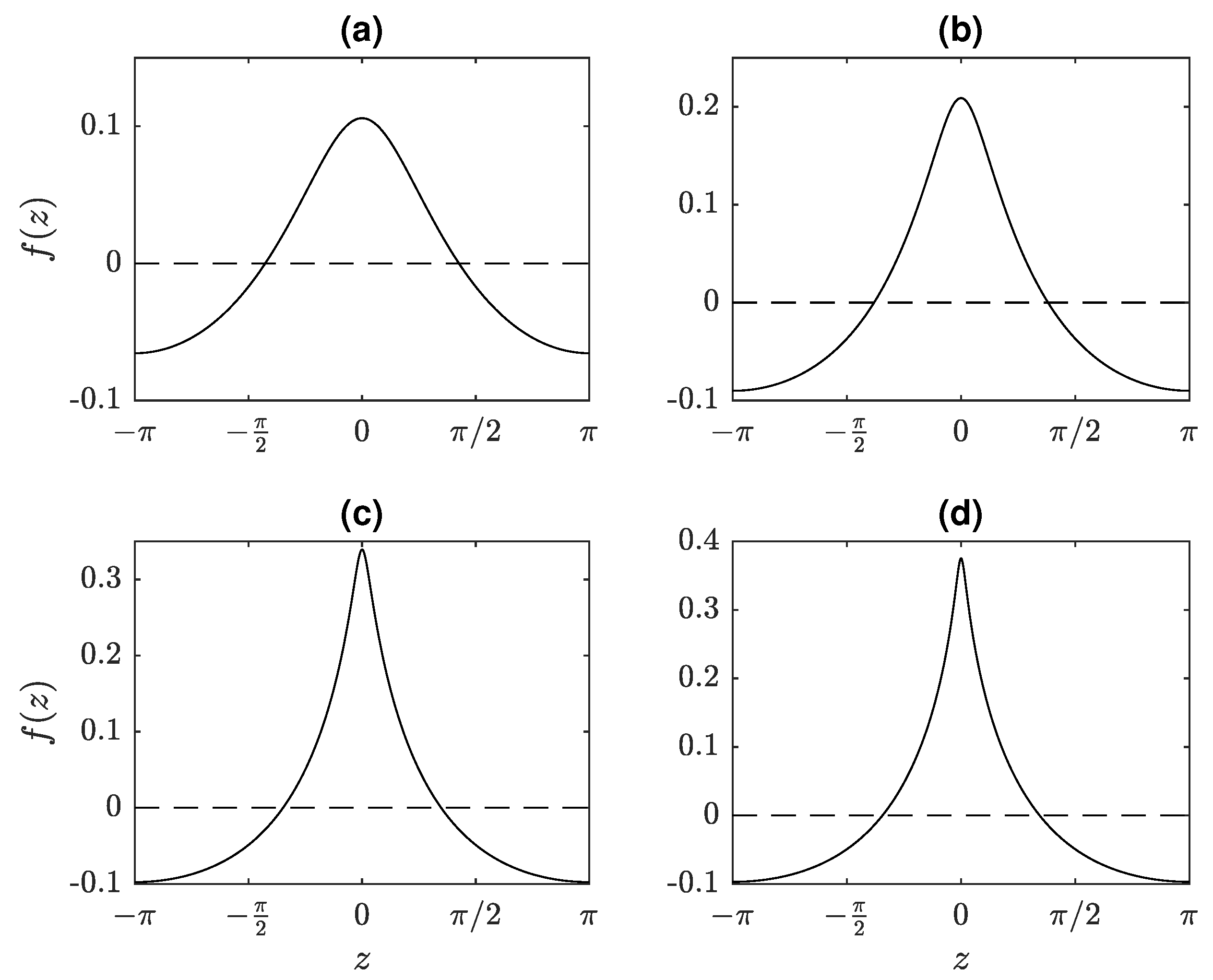
Figure 1.
Plots of four moderate wave height, -periodic, zero-mean solutions of the Whitham equation. The wave speeds and wave heights of these solutions are (a) , ; (b) , ; (c) , ; and (d) , . Note that the vertical scale is different in each of the plots.
Figure 1.
Plots of four moderate wave height, -periodic, zero-mean solutions of the Whitham equation. The wave speeds and wave heights of these solutions are (a) , ; (b) , ; (c) , ; and (d) , . Note that the vertical scale is different in each of the plots.
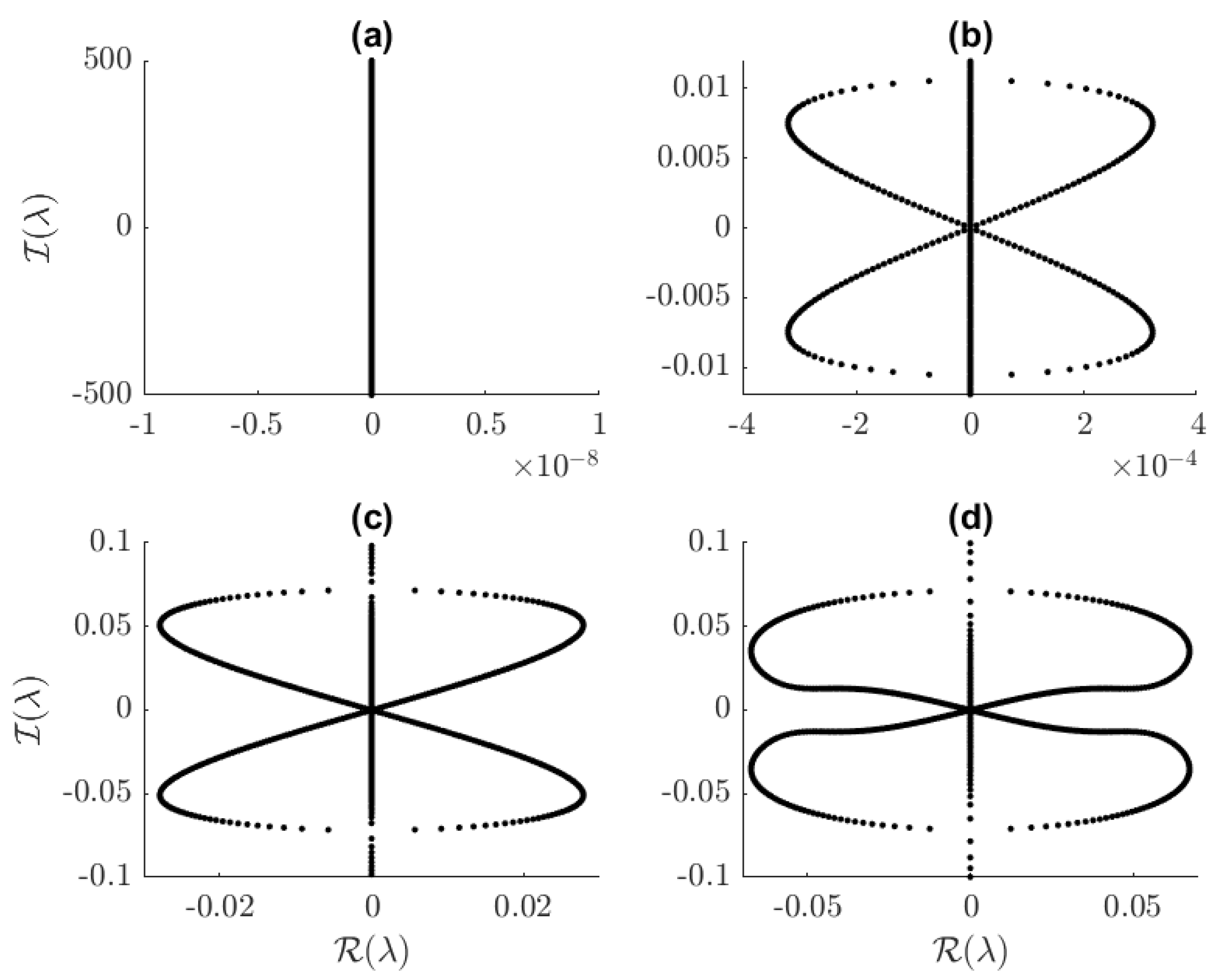
Figure 2.
Spectra of the solutions shown in
Figure 1. Note that both the horizontal and vertical scales vary from plot to plot.
Figure 2.
Spectra of the solutions shown in
Figure 1. Note that both the horizontal and vertical scales vary from plot to plot.
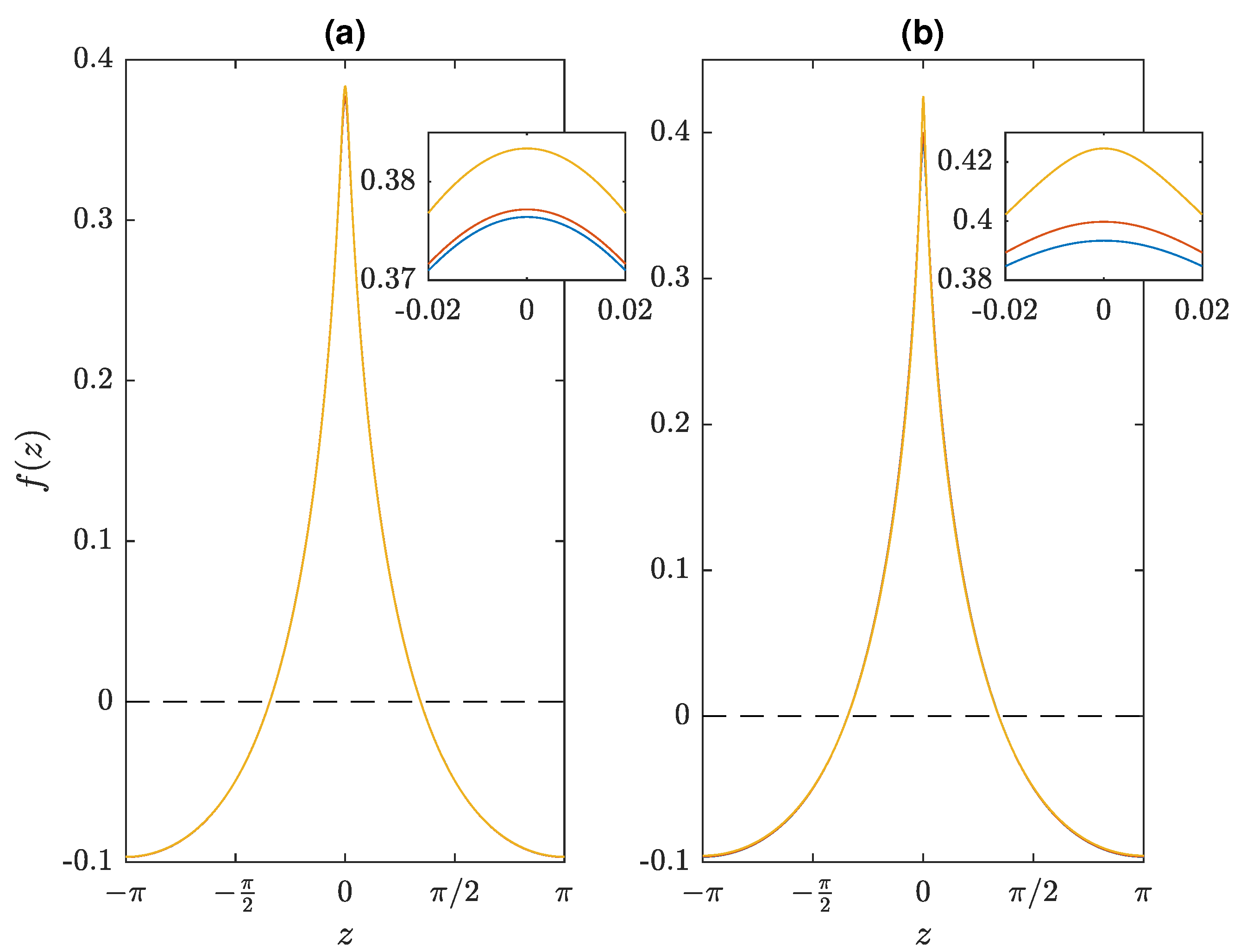
Figure 3.
(a) and (b) each contain three plots of large wave height, -periodic, zero-mean solutions of the Whitham equation. The solutions are very similar and nearly lie on top of one another. The inset plots are zooms of the intervals surrounding the crests of the solutions. The wave speeds and heights of these solutions, in order of increasing speed, are (a) and (blue); and (orange); and and (yellow); and (b) and (blue); and (orange); and and (yellow).
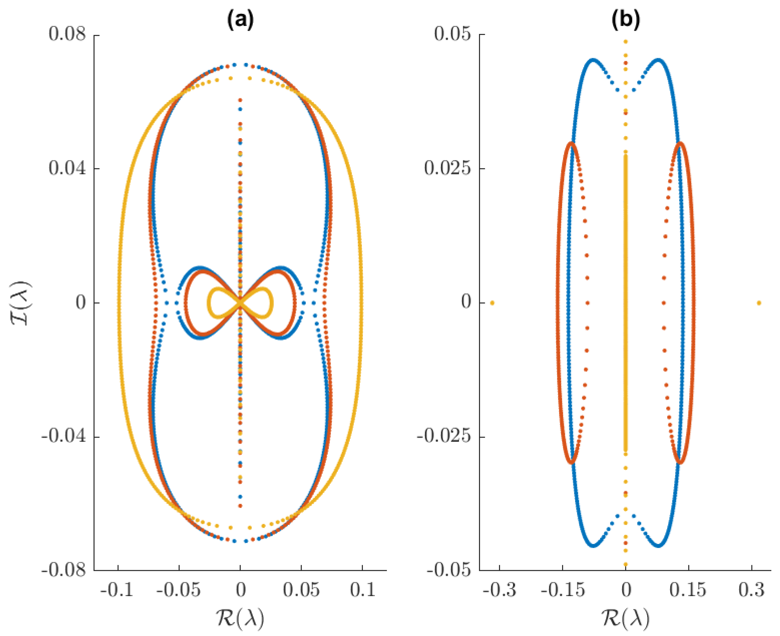
Figure 4.
Spectra of the solutions shown in
Figure 3.
Figure 4.
Spectra of the solutions shown in
Figure 3.
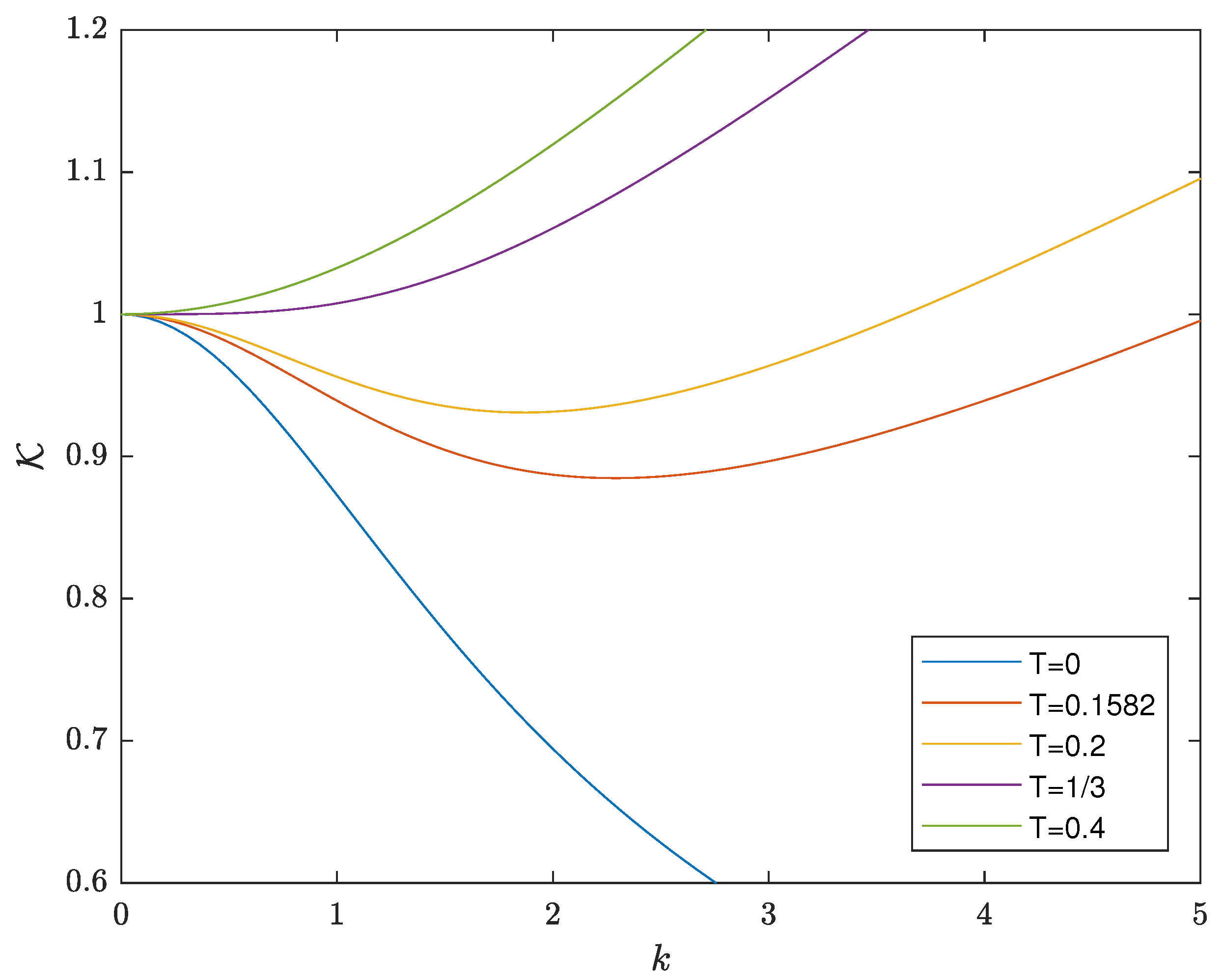
Figure 5.
Plots of versus k for each of the five values of T examined herein.
Figure 5.
Plots of versus k for each of the five values of T examined herein.
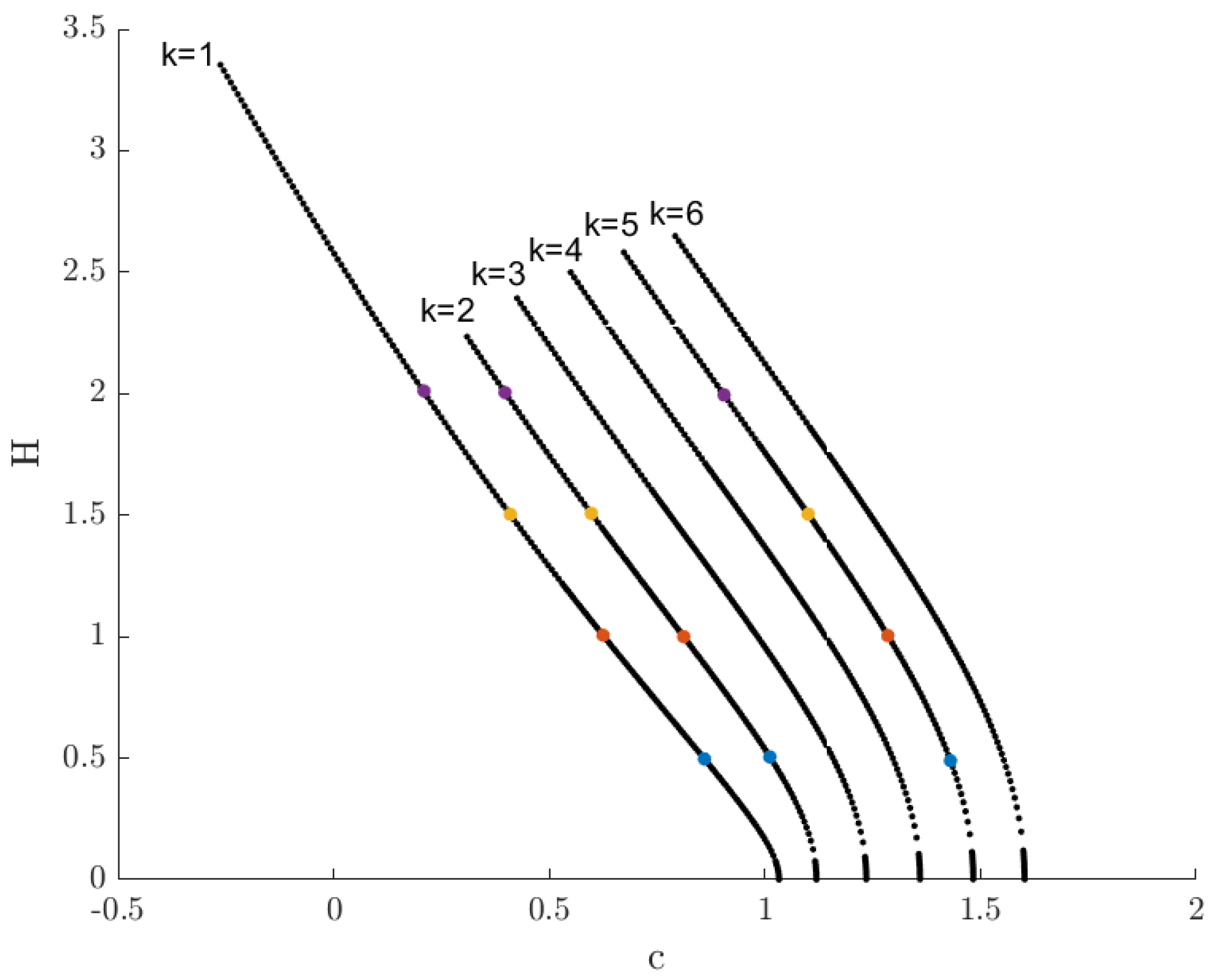
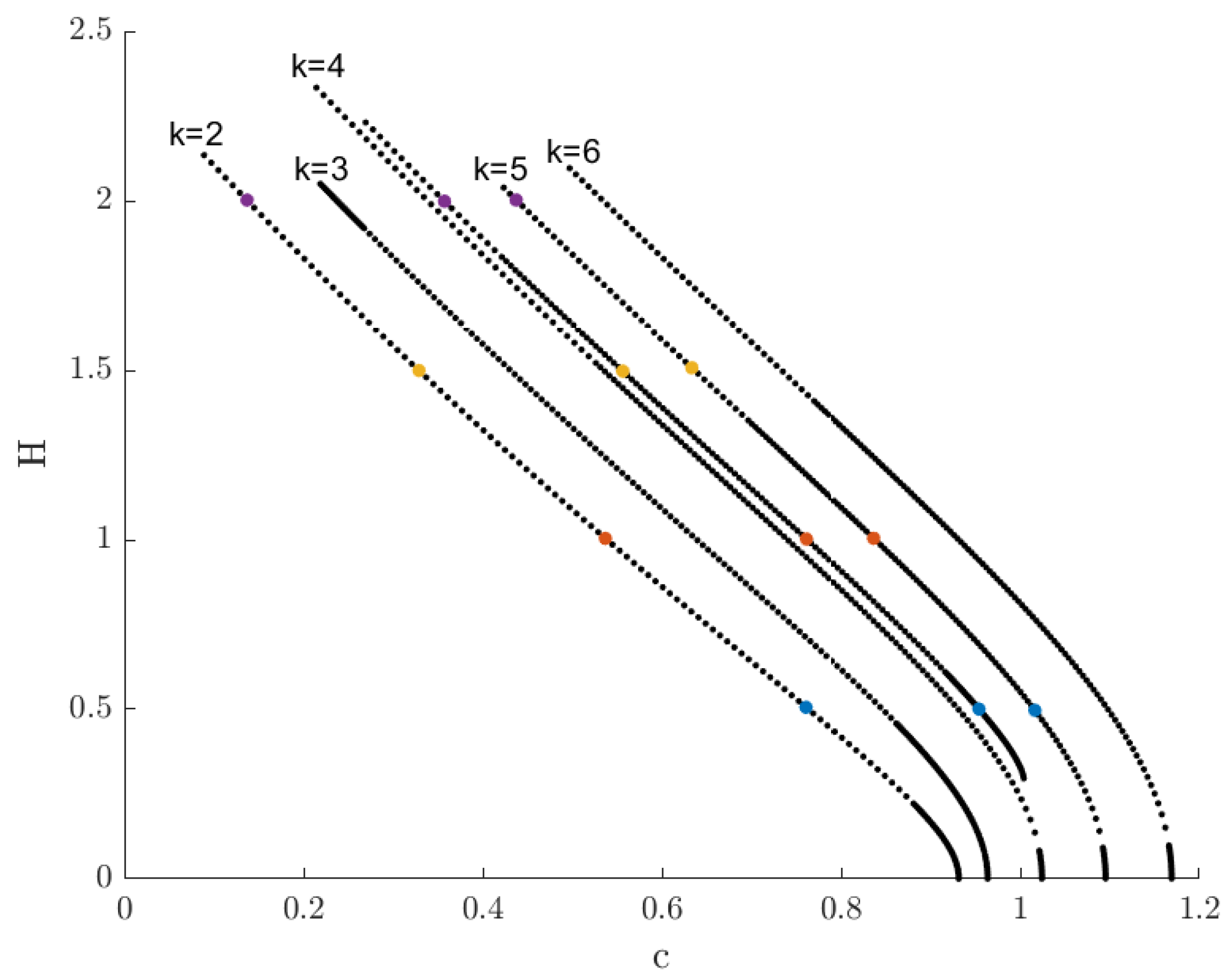
Figure 6.
A portion of the wave height versus wave speed bifurcation diagram for the capillary Whitham (cW) equation with
. The colored dots correspond to solutions that are examined in more detail in
Figure 7,
Figure 8 and
Figure 9.
Figure 6.
A portion of the wave height versus wave speed bifurcation diagram for the capillary Whitham (cW) equation with
. The colored dots correspond to solutions that are examined in more detail in
Figure 7,
Figure 8 and
Figure 9.
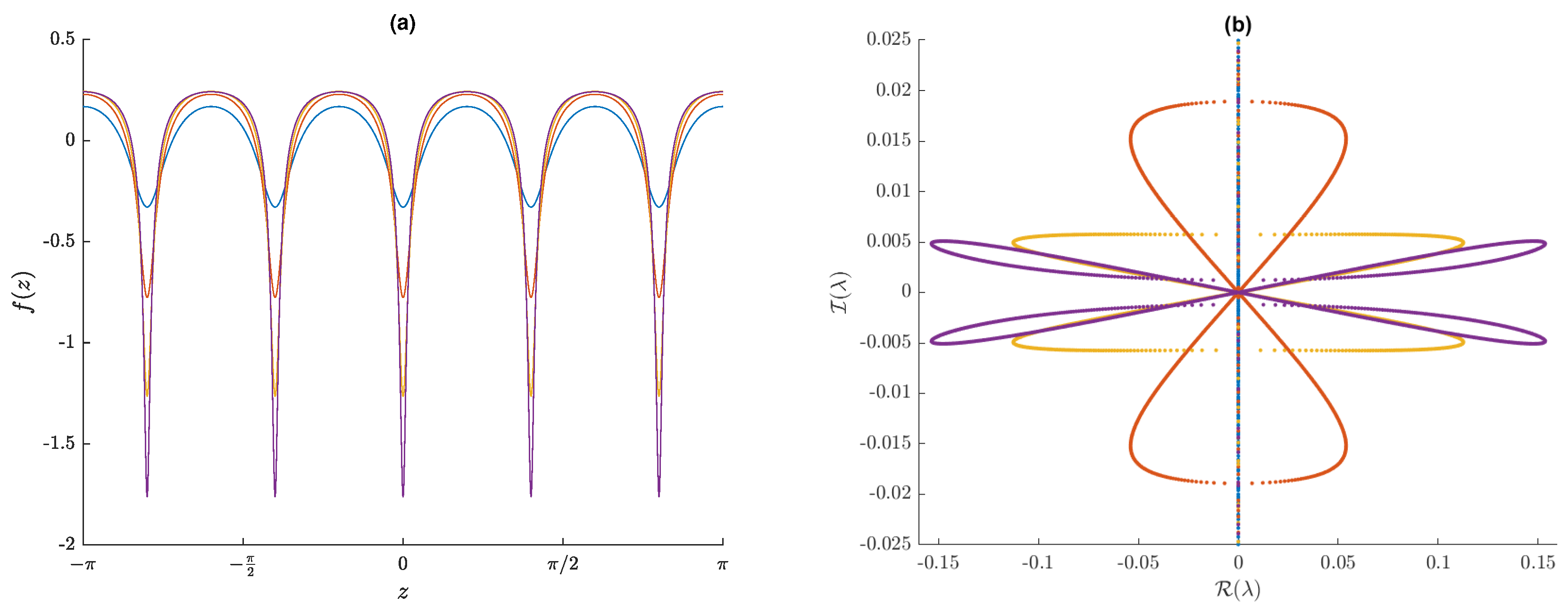
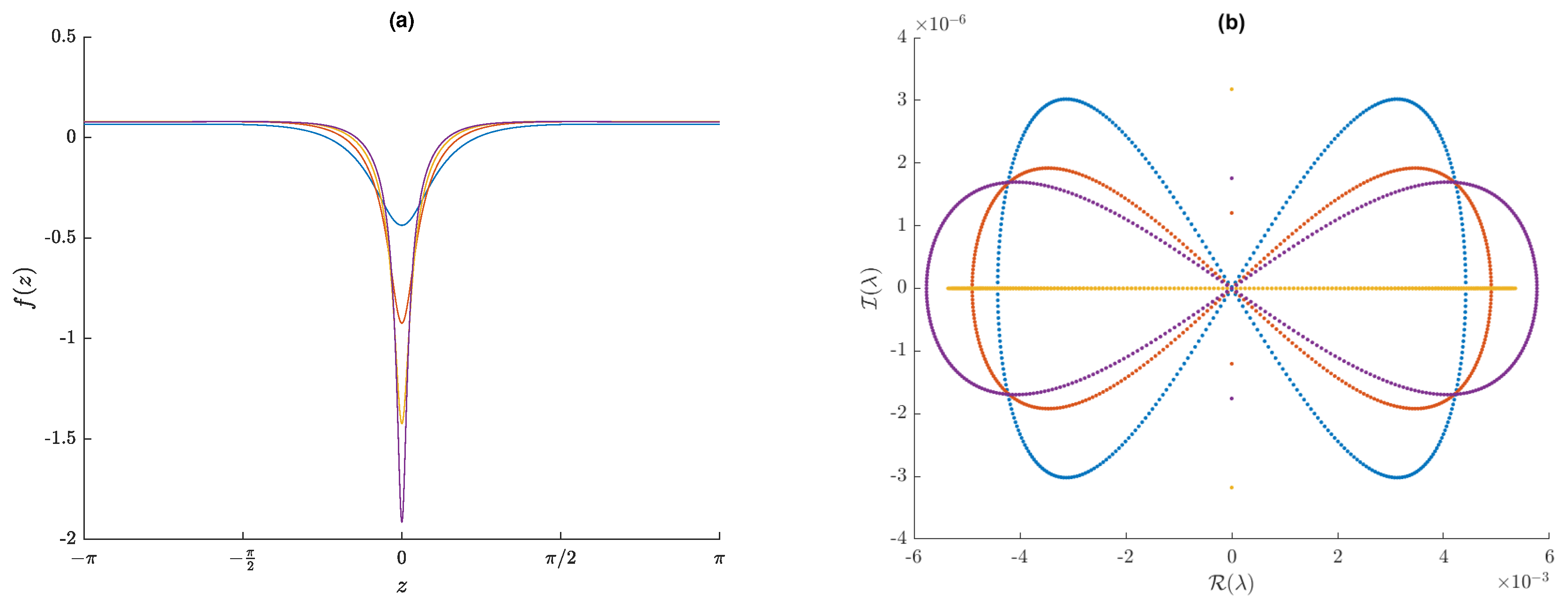
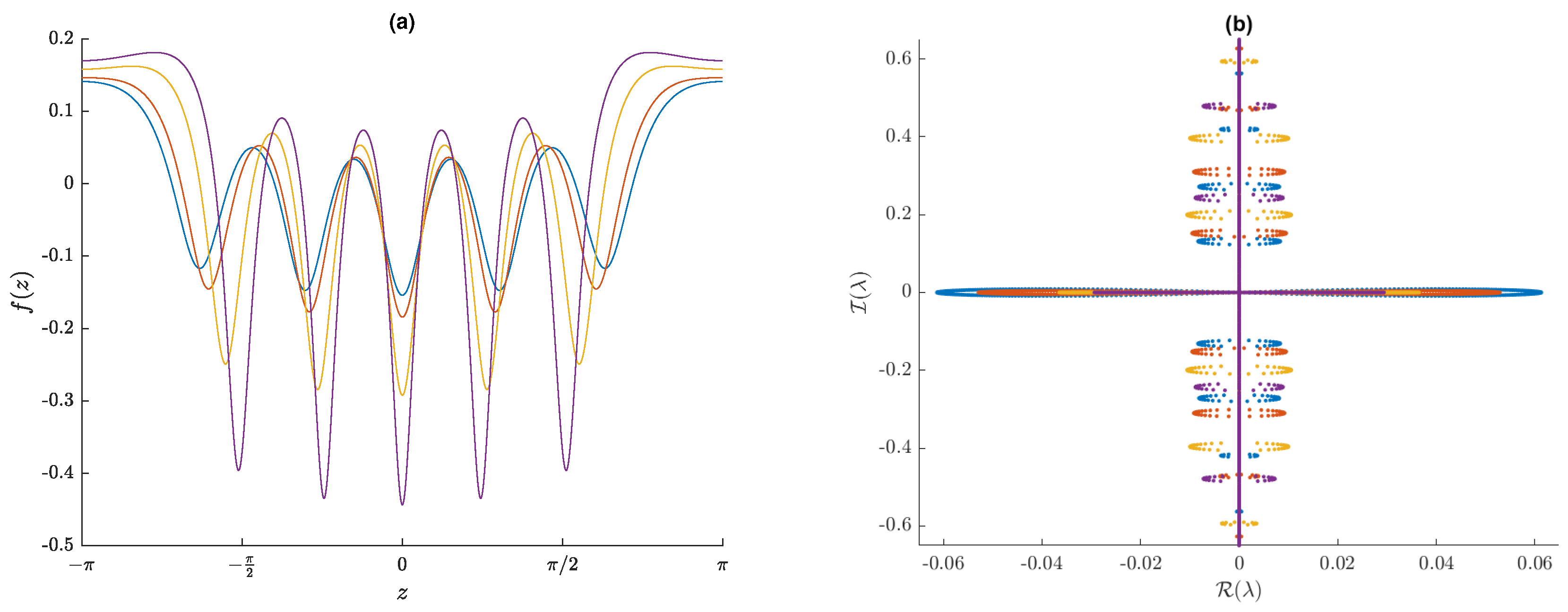
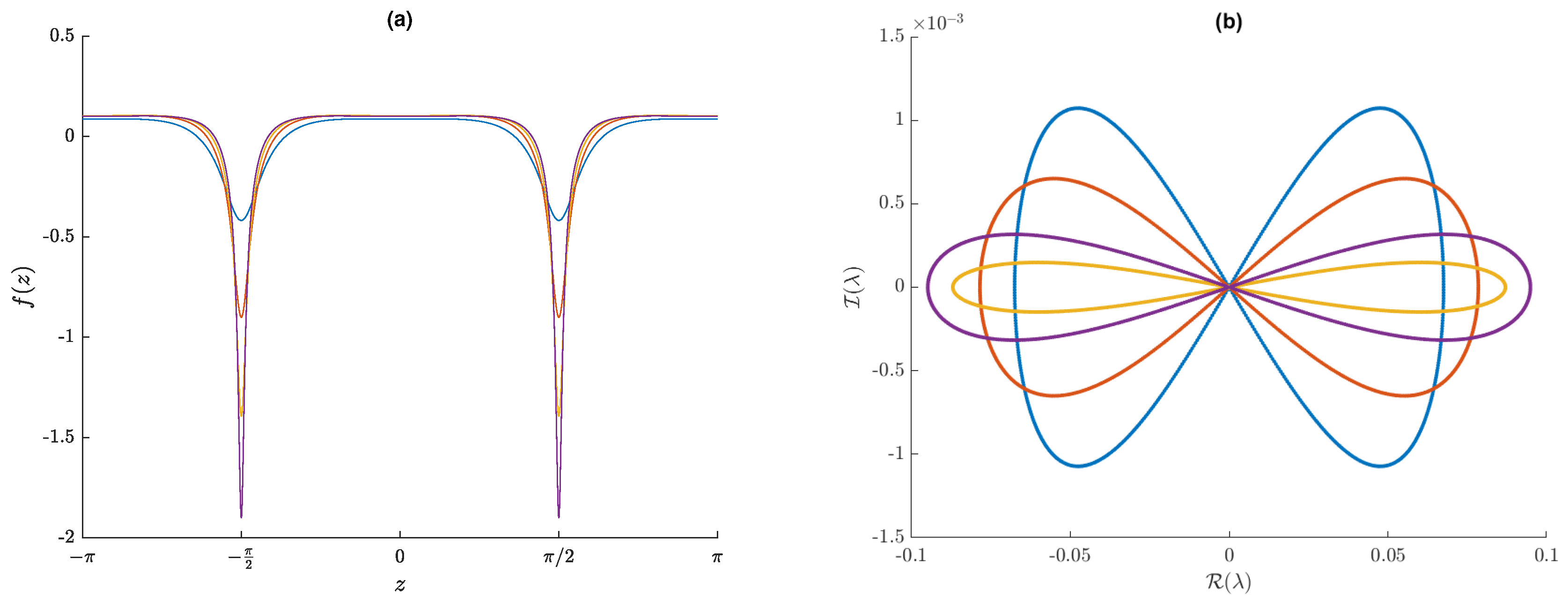
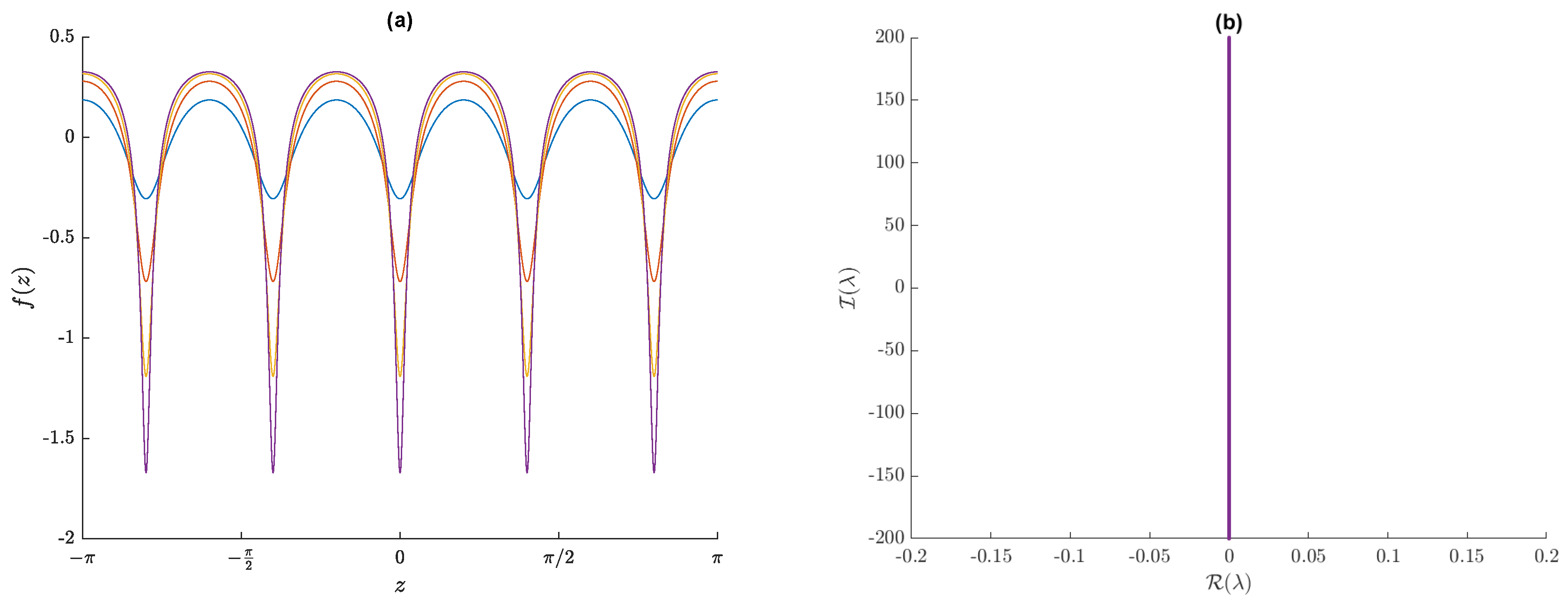
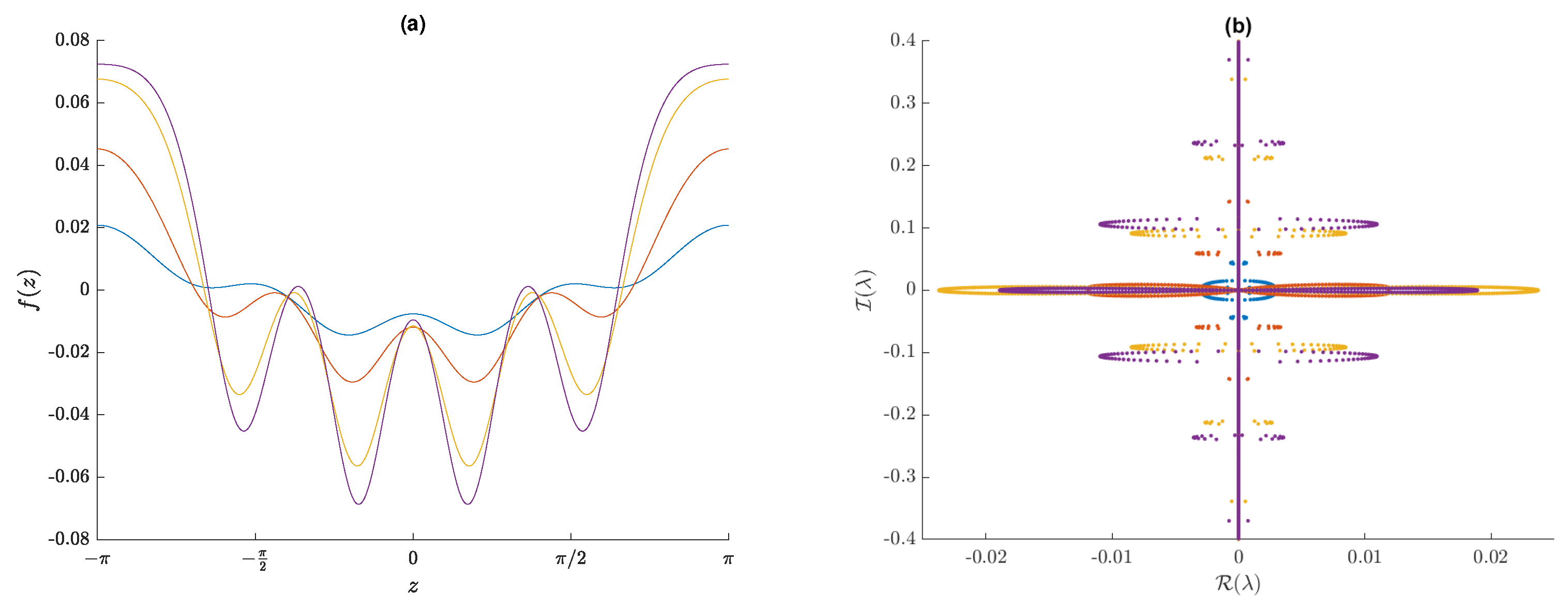
Figure 7.
Plots of (a) four representative solutions of the cW equation with and and (b) their stability spectra. The wave speeds and heights of these solutions are and (blue), and (orange), and (yellow), and and (purple).
Figure 7.
Plots of (a) four representative solutions of the cW equation with and and (b) their stability spectra. The wave speeds and heights of these solutions are and (blue), and (orange), and (yellow), and and (purple).
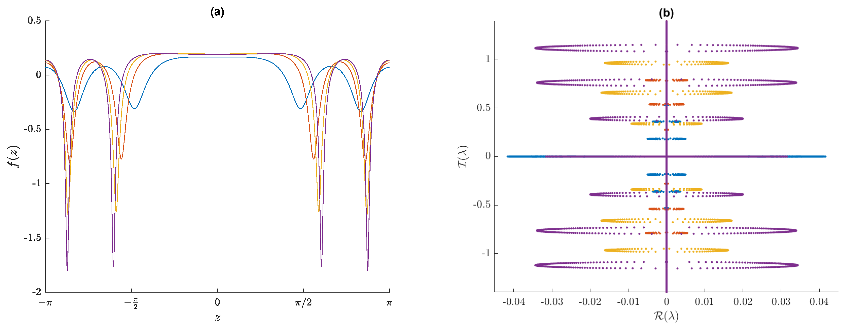
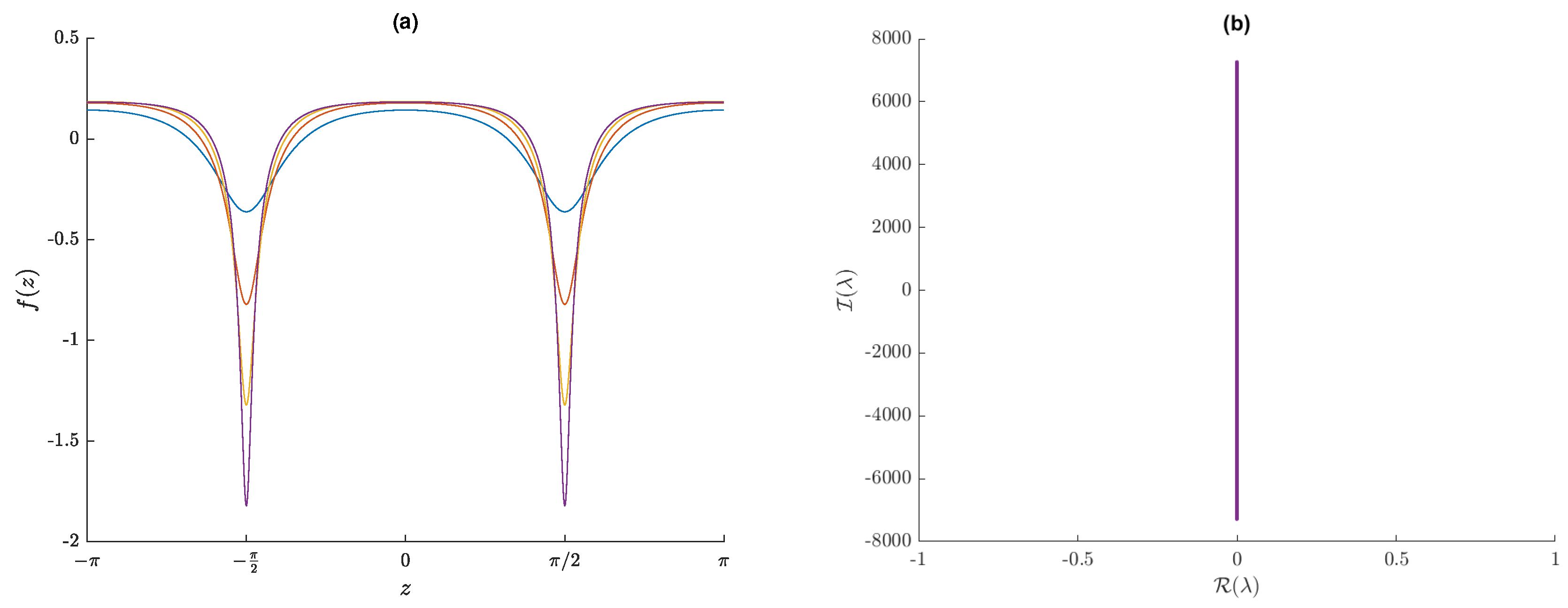
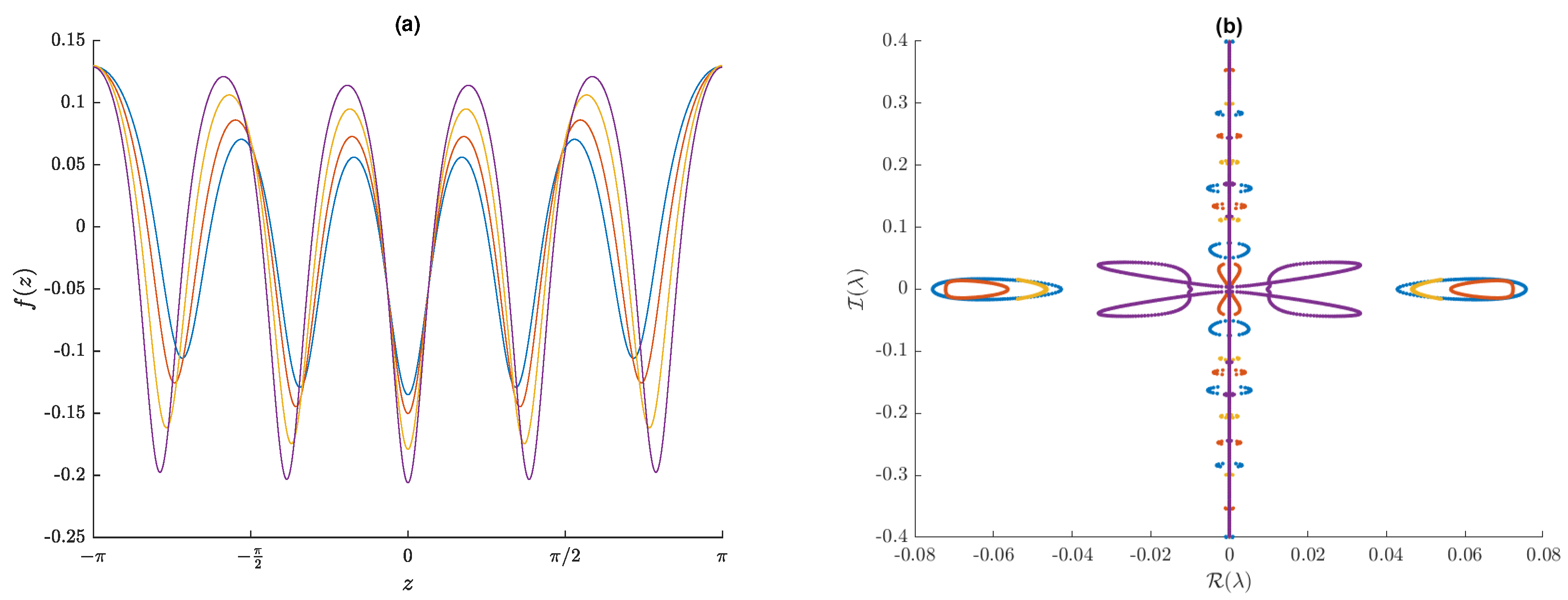
Figure 8.
Plots of (a) four representative solutions of the cW equation with and and (b) their stability spectra. The wave speeds and heights of these solutions are and (blue), and (orange), and (yellow), and and (purple).
Figure 8.
Plots of (a) four representative solutions of the cW equation with and and (b) their stability spectra. The wave speeds and heights of these solutions are and (blue), and (orange), and (yellow), and and (purple).
Figure 9.
Plots of (
a) four representative solutions of the cW equation with
from the solution branch that does not touch the horizontal axis in
Figure 6 and (
b) their stability spectra. The wave speeds and heights of these solutions are
and
(blue),
and
(orange),
and
(yellow), and
and
(purple).
Figure 9.
Plots of (
a) four representative solutions of the cW equation with
from the solution branch that does not touch the horizontal axis in
Figure 6 and (
b) their stability spectra. The wave speeds and heights of these solutions are
and
(blue),
and
(orange),
and
(yellow), and
and
(purple).
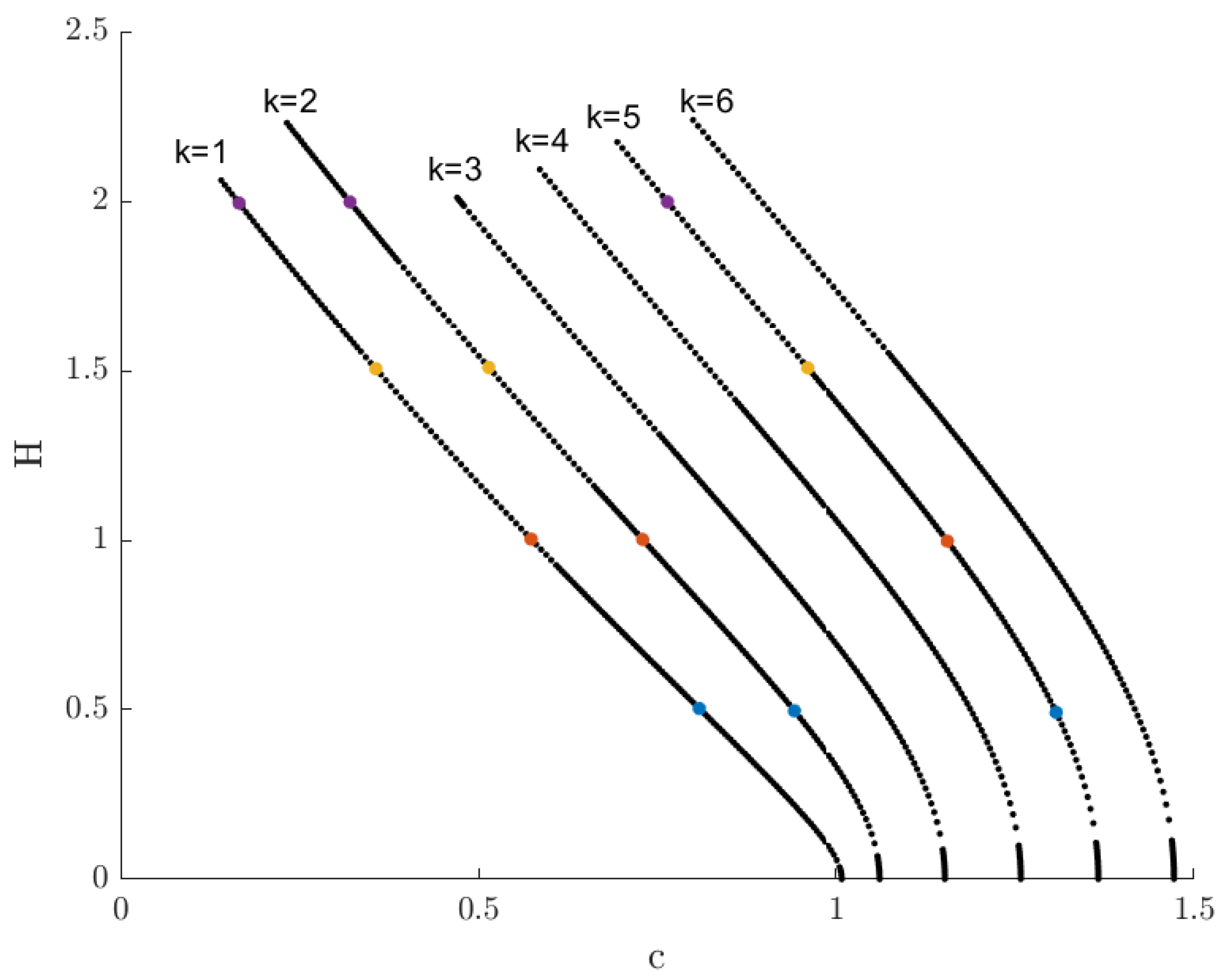
Figure 10.
A portion of the bifurcation diagram for the capillary Whitham equation with
. The colored dots correspond to solutions that are examined in more detail in
Figure 11,
Figure 12 and
Figure 13.
Figure 10.
A portion of the bifurcation diagram for the capillary Whitham equation with
. The colored dots correspond to solutions that are examined in more detail in
Figure 11,
Figure 12 and
Figure 13.
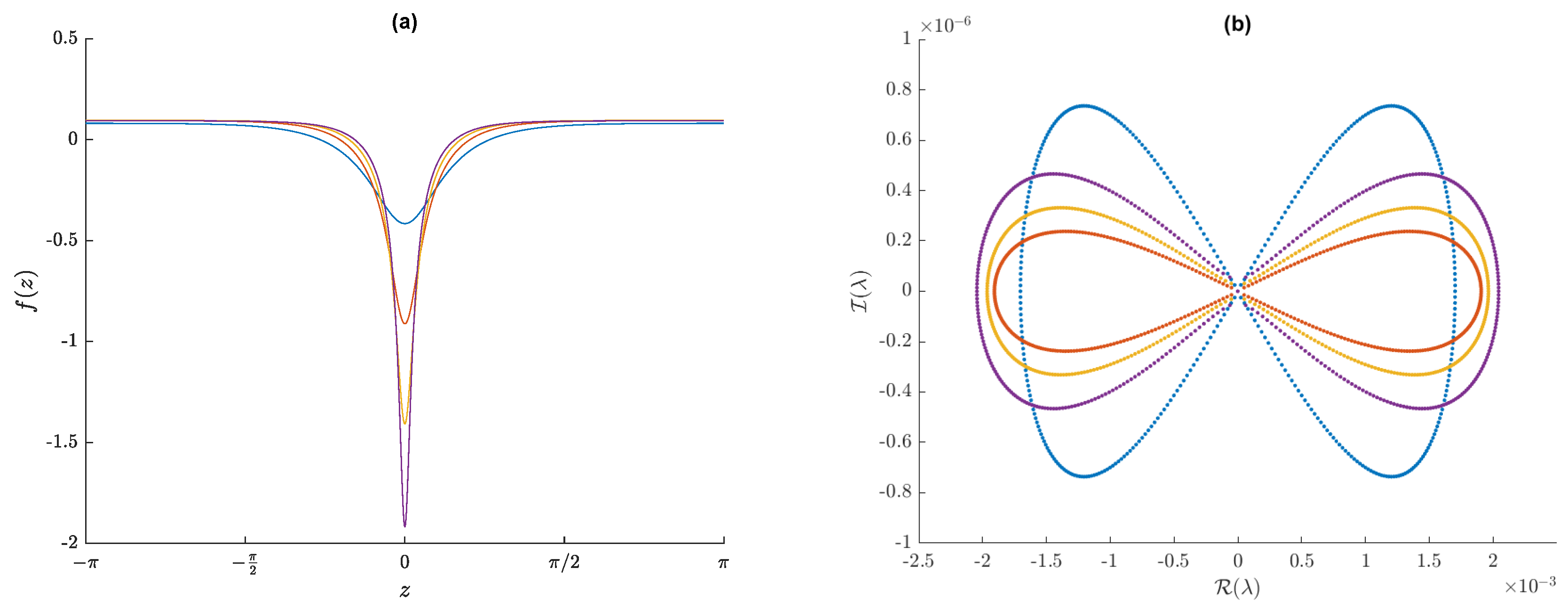
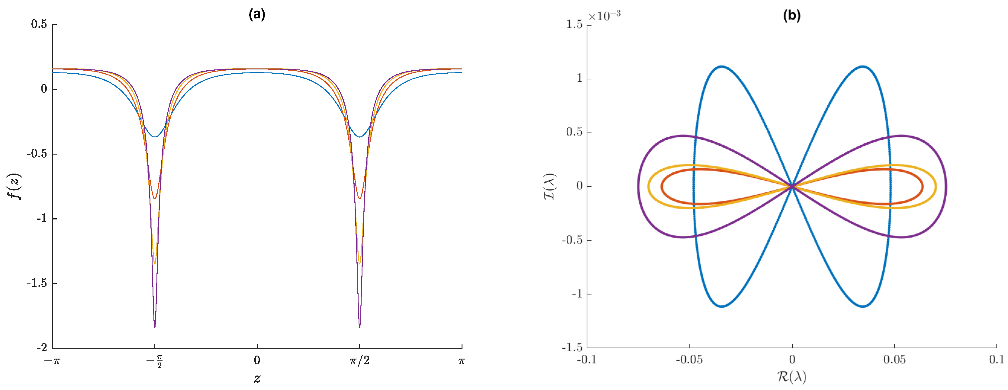
Figure 11.
Plots of (a) four representative solutions of the cW equation with and and (b) their stability spectra. The wave speeds and heights of these solutions are and (blue), and (orange), and (yellow), and and (purple).
Figure 11.
Plots of (a) four representative solutions of the cW equation with and and (b) their stability spectra. The wave speeds and heights of these solutions are and (blue), and (orange), and (yellow), and and (purple).
Figure 12.
Plots of (a) four representative solutions of the cW equation with and and (b) their stability spectra. The wave speeds and heights of these solutions are and (blue), and (orange), and (yellow), and and (purple).
Figure 12.
Plots of (a) four representative solutions of the cW equation with and and (b) their stability spectra. The wave speeds and heights of these solutions are and (blue), and (orange), and (yellow), and and (purple).
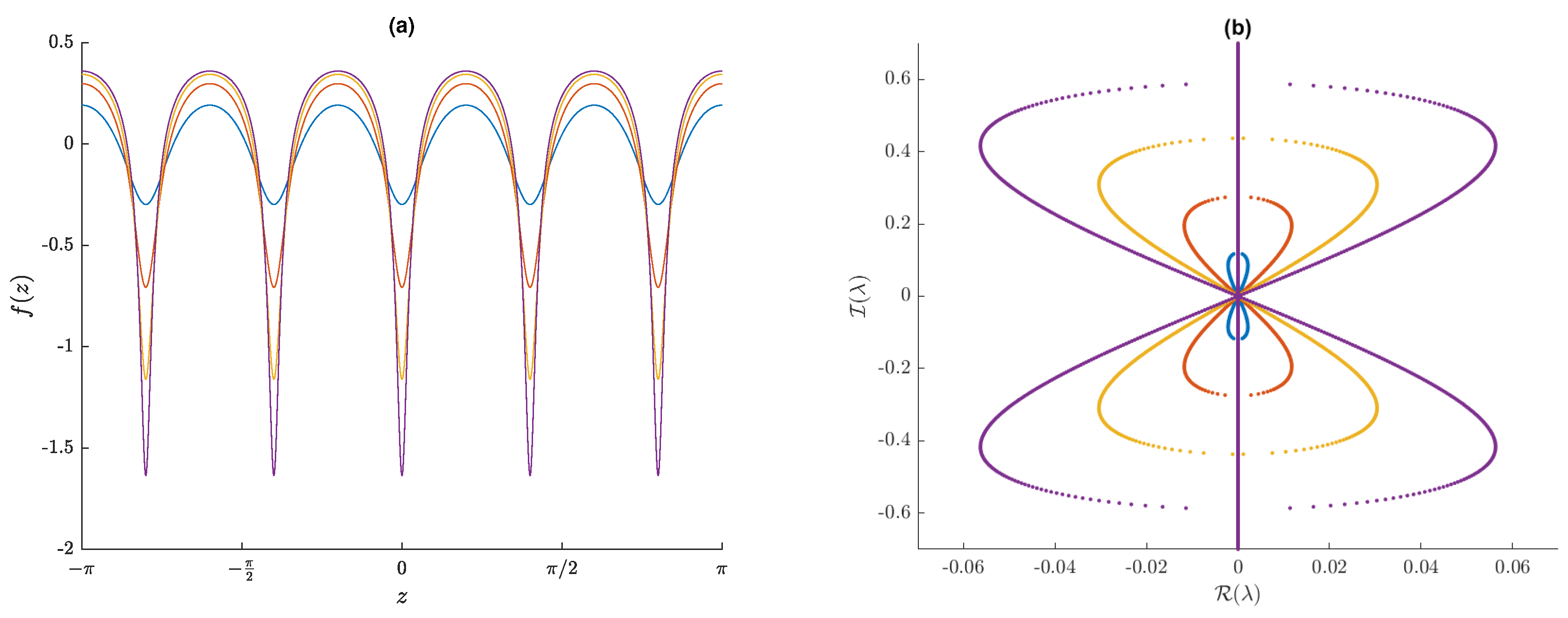
Figure 13.
Plots of (a) four representative solutions of the cW equation with and and (b) their stability spectra. The wave speeds and heights of these solutions are and (blue), and (orange), and (yellow), and and (purple).
Figure 13.
Plots of (a) four representative solutions of the cW equation with and and (b) their stability spectra. The wave speeds and heights of these solutions are and (blue), and (orange), and (yellow), and and (purple).
Figure 14.
A portion of the bifurcation diagram for the cW equation with
. The colored dots correspond to solutions that are examined in more detail in
Figure 15,
Figure 16 and
Figure 17.
Figure 14.
A portion of the bifurcation diagram for the cW equation with
. The colored dots correspond to solutions that are examined in more detail in
Figure 15,
Figure 16 and
Figure 17.
Figure 15.
Plots of (a) four representative solutions of the cW equation with and and (b) their stability spectra. The wave speeds and heights of these solutions are and (blue), and (orange), and (yellow), and and (purple).
Figure 15.
Plots of (a) four representative solutions of the cW equation with and and (b) their stability spectra. The wave speeds and heights of these solutions are and (blue), and (orange), and (yellow), and and (purple).
Figure 16.
Plots of (a) four representative solutions of the cW equation with and and (b) their stability spectra. The wave speeds and heights of these solutions are and (blue), and (orange), and (yellow), and and (purple).
Figure 16.
Plots of (a) four representative solutions of the cW equation with and and (b) their stability spectra. The wave speeds and heights of these solutions are and (blue), and (orange), and (yellow), and and (purple).
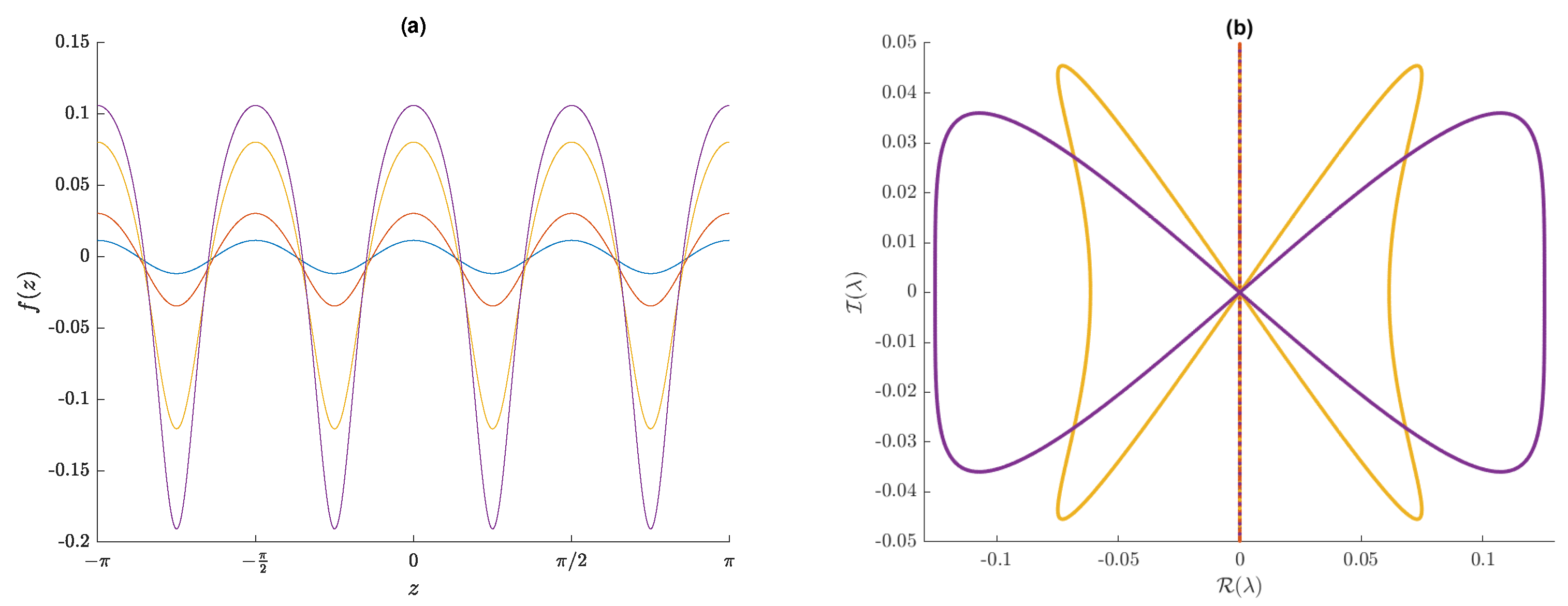
Figure 17.
Plots of (a) four representative solutions of the cW equation with and and (b) their stability spectra. The wave speeds and heights of these solutions are and (blue), and (orange), and (yellow), and and (purple).
Figure 17.
Plots of (a) four representative solutions of the cW equation with and and (b) their stability spectra. The wave speeds and heights of these solutions are and (blue), and (orange), and (yellow), and and (purple).
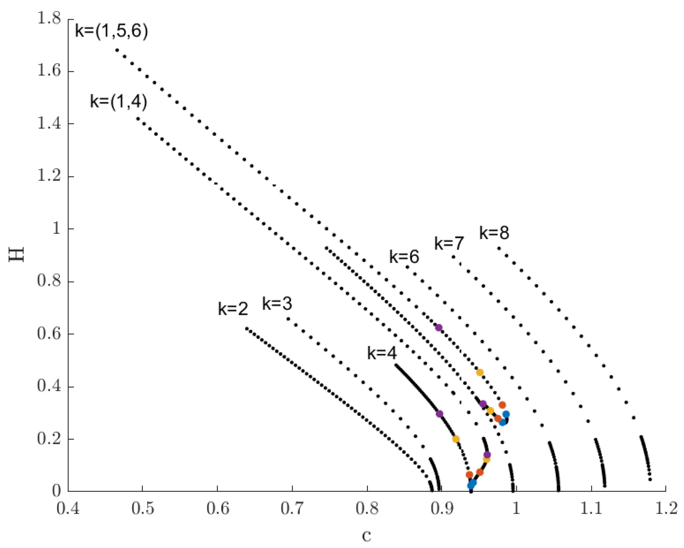
Figure 18.
A portion of the bifurcation diagram for the cW equation with
. The colored dots correspond to solutions that are examined in more detail in
Figure 19,
Figure 20,
Figure 21 and
Figure 22.
Figure 18.
A portion of the bifurcation diagram for the cW equation with
. The colored dots correspond to solutions that are examined in more detail in
Figure 19,
Figure 20,
Figure 21 and
Figure 22.
Figure 19.
Plots of (a) four representative solutions of the cW equation with and and (b) their stability spectra.
Figure 19.
Plots of (a) four representative solutions of the cW equation with and and (b) their stability spectra.
Figure 20.
Plots of (a) four representative solutions of the cW equation with and and (b) their stability spectra.
Figure 20.
Plots of (a) four representative solutions of the cW equation with and and (b) their stability spectra.
Figure 21.
Plots of (a) four representative solutions of the cW equation with and and (b) their stability spectra.
Figure 21.
Plots of (a) four representative solutions of the cW equation with and and (b) their stability spectra.
Figure 22.
Plots of (a) four representative solutions of the cW equation with and and (b) their stability spectra.
Figure 22.
Plots of (a) four representative solutions of the cW equation with and and (b) their stability spectra.
Table 1.
A summary of stability results for single-mode, periodic, traveling-wave solutions with period , wavenumber k, and surface tension parameter T. The first letter in each cell signifies if small-amplitude solutions are spectrally stable (s) or unstable (u). The second letter in each cell signifies if moderate- and large-amplitude solutions are spectrally stable or unstable. We were unable to compute the solutions corresponding to the cells that are left blank.
| | | | | | |
|---|
| su | uu | uu | uu | uu |
| | uu | uu | su | su |
| | uu | uu | uu | su |
| uu | uu | ss | ss | ss |
| uu | ss | ss | ss | uu |


