Article

A Model for Fuel Spray Formation with Atomizing Air

1
Department of Mechanical and Aeronautical Engineering, Clarkson University, Potsdam, NY 13699, USA
2
Scientific Computing, Research & Engineering IT, ExxonMobil Technical Computing Company, Annandale, NJ 08801, USA
3
NextEra energy, Juno Beach, FL 33408, USA
*
Author to whom correspondence should be addressed.
Fluids 2019, 4(1), 20; https://doi.org/10.3390/fluids4010020
Submission received: 28 November 2018 / Revised: 12 January 2019 / Accepted: 19 January 2019 / Published: 29 January 2019

Abstract

:
The formation of a liquid spray emanating from a nozzle in the presence of atomizing air was studied using a computational model approach that accounted for the deformation and break up of droplets. Particular attention was given to the formation of sprays under non-swirling flow conditions. The instantaneous fluctuating fluid velocity and velocity gradient components were evaluated with the use of a probability density function (PDF)-based Langevin equation. Motions of atomized fuel droplets were analyzed, and ensemble and time averaging were used for evaluating the statistical properties of the spray. Effects of shape change of droplets, and their breakup, as well as evaporation, were included in the model. The simulation results showed that the mean-square fluctuation velocities of the droplets vary significantly with their size and shape. Furthermore, the mean-square fluctuation velocities of the evaporating droplet differed somewhat from non-evaporating droplets. Droplet turbulence diffusivities, however, were found to be close to the diffusivity of fluid point particles. The droplet velocity, concentration, and size of the simulated spray were compared with the experimental data and reasonable agreement was found.

1. Introduction

Understanding the formation and subsequent dynamics of turbulent liquid sprays are of considerable interest to the design and operation of jet and rocket engines. However, the large range of length and time scales over which these liquid sprays form and evolve lead to considerable computational complexities. Therefore, there have been numerous studies in the literature on various aspects of spray processes.
Extensive reviews on turbulent spray combustion were reported by Faeth [1] and Law [2] and more recently by Jiang et al. [3] and Gutheil [4] and Jenny et al. [5]. Shang et al. [6] and Berlemont et al. [7] presented the procedure for Lagrangian simulation of droplet evaporation in turbulent flows. Kvasnak et al. [8] included the effect of droplet deformation and breakup to their models. Recent advances for using Eulerian-Lagrangian approach for spray modelling was reported by Kolakaluri et al. [9], Keller et al. [10], and Doisneau et al. [11], among others. Hoyas et al. [12] performed two-dimensional Eulerian-Lagrangian spray simulations in the near-nozzle region.
Large eddy simulations (LES) of atomizing spray were reported by Apte et al. [13], Jones and Lettieri [14], Irannejad et al. [15], Jones et al. [16], Khan et al. [17] and Noh et al. [18]. Li et al. [19] performed Large-Eddy simulations of ethanol spray combustion. Senoner et al. [20], Prasad et al. [21], and Li et al. [19] compared the Eulerian-Lagrangian simulation results using different LES solvers. Earlier, McDonell and Samuelsen [22] provided experimental data on droplet size and velocity distributions in a simplex atomizer.
Kvasnak et al. [8] examined the formation of liquid sprays in the absence of atomizing air. Their analysis included effects of primary breakup for liquid ellipsoidal droplets based on the Taylor Analogy Breakup (TAB) model developed by O’Rourke and Amsden [23], and later modified by Ibrahim [24], and Kvasnak and Ahmadi [25]. Recent reviews of the spray simulation and breakup methods were presented by Jenny et al. [5].
This work was concerned with understanding the effects of droplet deformation, breakup, and evaporation on the dispersion of deforming ellipsoidal spray droplets in turbulent fuel injector flow fields with atomizing air, with a focus towards practical applications. The other goal was to develop a computational tool for the simulation of practical liquid spray fuel injectors. Kvasnak et al. [8] described a detailed numerical procedure for generating ensembles of simultaneous sample particle trajectories for estimating particle velocity and dispersion statistics. The presented study showed that, in many cases of practical importance to fuel injectors with atomizing air, the deformation time scale of the fuel droplets was comparable with their evaporation time scale. The droplet nonsphericity was also found to be an important factor for modeling the fuel injector performance. The simulation results were compared with the experimental data of McDonell and Samuelsen [22] for a simplex atomizer with atomizing air, where qualitative agreement was found.

2. Governing Equations

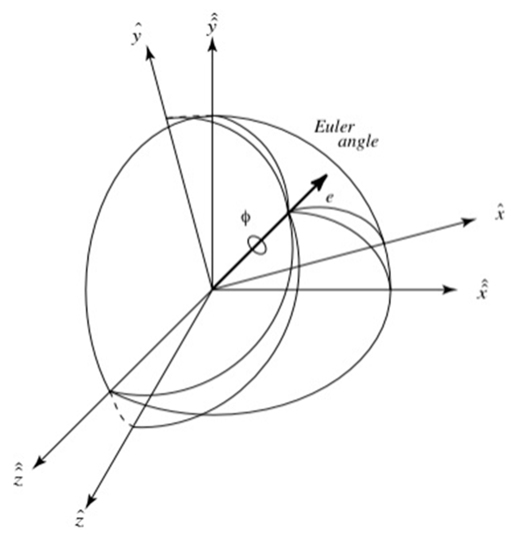
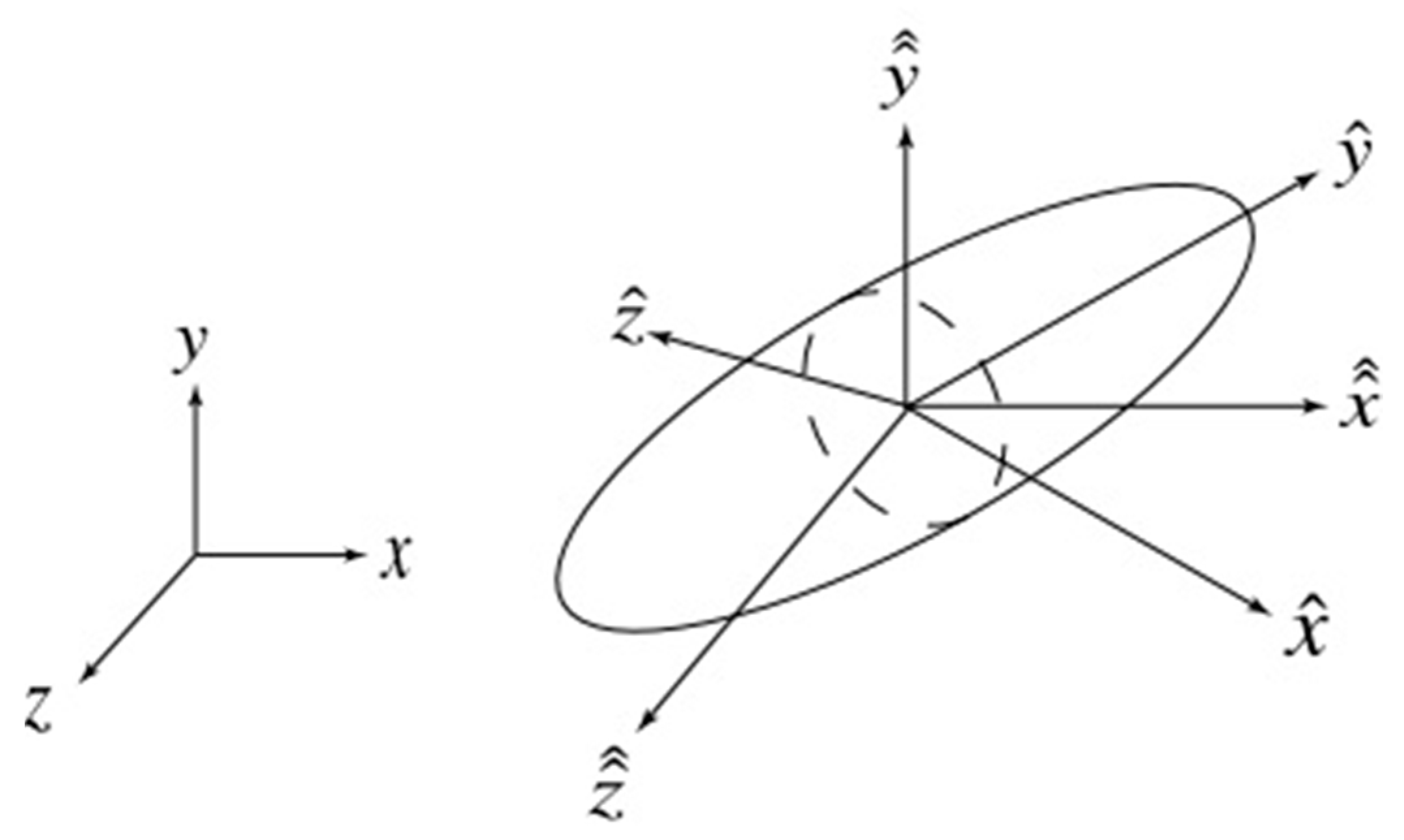
2.1. Equations of Motion for Ellipsoidal Particles

In this section, the equations of motion for an ellipsoid of revolution suspended in a turbulent velocity field as described by Fan and Ahmadi [26] and Zhang et al. [27] are outlined. Figure 1 shows the schematic of an ellipsoidal particle moving in a general flow field and the corresponding inertial ( x , y , z ) and particle ( x ^ , y ^ , z ^ ) coordinate systems. The co-motion frame, ( x ^ ^ , y ^ ^ , z ^ ^ ), with its origin being at the particle centroid and having axes parallel to the inertial frame, is also shown in this figure.
The equations of motion of a non-spherical rigid particle moving in an arbitrary flow field, in the presence of hydrodynamic and gravitational forces are given as Goldstein [28], and Gallily and Cohen [29].

2.1.1. Translational Motion

m p d v d t = f h + f L + m p g ,

2.1.2. Rotational Motion

I x ^ d ω x ^ d t ω y ^ ω z ^ ( I y ^ I z ^ ) = T x ^ h ,
I y ^ d ω y ^ d t ω z ^ ω x ^ ( I z ^ I x ^ ) = T y ^ h ,
I z ^ d ω z ^ d t ω x ^ ω y ^ ( I x ^ I y ^ ) = T z ^ h .
Here, m p is the mass of the particle, t is the time, v is the translational velocity vector acting at the particle center of gravity, f h is the hydrodynamic drag force acting on the particle, f L is the lift force, and g is the acceleration of body force (i.e., gravity). In Equations (2)–(4), I x ^ , I y ^ , I z ^ are the moments of inertia of the particle with respect to the particle principal axes, ω x ^ , ω y ^ , ω z ^ are the angular velocities of the particle with respect to the principal particle axes, and T x ^ h , T y ^ h , T z ^ h are the components of the hydrodynamic torque acting on the particle. Equation (1) expresses the translational motion in the inertial frame, ( x , y , z ) , while Equations (2)–(4) for the rotational motion are stated in the particle frame, ( x ^ , y ^ , z ^ ). It should be emphasized that Equations (2)–(4) are for rigid bodies. Here, it is assumed that these equations are approximately valid for droplets with high viscosity.
The particle position may be easily obtained by integrating
d x d t = v ,
where x = ( x , y , z ) is the position vector. Evaluation of the particle orientation, however, is more complicated. Recognizing that the rotational motion is written in particle coordinates, a change of frame is required. The transformation between the co-motion and the particle frame of reference was given by Goldstein [28] as
x ^ = A x ^ ^ ,
where x ^ = ( x ^ , y ^ , z ^ ) and x ^ ^ = ( x ^ ^ , y ^ ^ , z ^ ^ ) , and A is the transformation matrix.
Fan and Ahmadi [26] showed that the Euler four parameters or quaternions may be used to avoid the singularity produced by the use of Euler’s angles for full rotational motion of a rigid body. Here, the Euler four parameters, shown in Figure 2, are defined as
[ ε 1 , ε 2 , ε 3 ] T = e sin ( ϕ 2 ) ,
η = cos ( ϕ 2 ) ,
where e is the unit vector along the axis of rotation, ϕ is the angle of rotation, and the superscript T denotes a matrix transpose. Because the most general rotation of a rigid body has only three degrees of freedom, Euler’s four parameters are subject to a constraint given as
ε 1 2 + ε 2 2 + ε 3 3 + η 2 = 1 .
The transformation matrix A in Equation (6) may be stated in terms of quaternions as Hughes [30],
A = [ 1 2 ( ε 2 2 + ε 3 2 ) 2 ( ε 1 ε 2 + ε 3 η ) 2 ( ε 1 ε 3 ε 2 η ) 2 ( ε 2 ε 1 ε 3 η ) 1 2 ( ε 3 2 + ε 1 2 ) 2 ( ε 2 ε 3 + ε 1 η ) 2 ( ε 3 ε 1 + ε 2 η ) 2 ( ε 3 ε 2 ε 1 η ) 1 2 ( ε 1 2 + ε 2 2 ) ] .
The time rates of change of quaternions are given by
[ d ε 1 / d t d ε 2 / d t d ε 3 / d t d η / d t ] = 1 2 [ η ω x ^ ε 3 ω y ^ + ε 2 ω z ^ ε 3 ω x ^ + η ω y ^ ε 1 ω z ^ ε 2 ω x ^ + ε 1 ω y ^ + η ω z ^ ε 1 ω x ^ ε 2 ω y ^ ε 3 ω z ^ ] .
The initial conditions of the quaternions are obtained from the initial direction cosines, a i j , by the following relations: If η 0 ,
η = ± 1 2 ( 1 + a 11 + a 22 + a 33 ) 1 2 ,
[ ε 1 ε 2 ε 3 ] = 1 4 η [ a 23 a 32 a 31 a 13 a 12 a 21 ] .
The non-uniqueness given by Equations (12) and (13) does not introduce any difficulty because all solutions correspond to the same transformation matrix and result in identical particle trajectories.

2.2. Ellipsoids of Revolution

Ellipsoids of revolution cover a wide variety of particle shapes (e.g., spheres, prolate spheroids, and oblate spheroids). In fact, all quadratic surfaces of finite extent are, by definition, ellipsoids. A particle entrained in a viscous fluid is subject to various hydrodynamic forces and torques such as drag, lift, Faxen, Bassett history, etc. In this work, only the leading order hydrodynamic forces of drag and lift are included in the equations of motion for small ellipsoidal particles. Explicit expressions for the hydrodynamic forces and torques for an ellipsoid of revolution are described in this section. Throughout this paper, the y-axis is assumed to be along the particle major axis as shown in Figure 1.

2.3. Nonlinear Hydrodynamic Drag

The general hydrodynamic forces and torques acting on an ellipsoidal particle in an arbitrary creeping flow field were described by Happel and Brenner [31]. For larger particles moving outside of the creeping flow regime, certain Reynolds number corrections are needed. Here,
f h = π μ a 1 + B ( 1 + 0.24 R e a 0.687 ) K ^ ^ ( u v )
for evaporating ellipsoidal droplets is used. In this equation, μ is the viscosity of the fluid, B is the Spalding transfer number for evaporating droplets, and Rea is the particle Reynolds number based on the minimum radius of the particle and the flow/particle velocity difference. This equation is a simple generalization of the nonlinear drag for a sphere to ellipsoids. The Spalding transfer number correction to the coefficient of drag is also a simple extension from the spherical case. The particle Reynolds number is defined as
R e a = a | u v | ν ,
where u = (ux,uy,uz) is the flow velocity vector at the centroid of the particle in the absence of the particle, and ν is the kinematic viscosity of the fluid.
In Equation (14), a double hat denotes a quantity expressed in the co-motion frame. The transformation of the translation matrix is given by
K ^ ^ = A 1 K ^ A .
The particle-frame translation matrix K ^ for an ellipsoid of revolution is a diagonal matrix, i.e.,
K ^ = [ K x ^ x ^ 0 0 0 K y ^ y ^ 0 0 0 K z ^ z ^ ] ,
with
K x ^ x ^ = K z ^ z ^ = 16 π a ( β 2 1 ) ( λ + 2 / 3 λ + 1 ) [ ( 2 β 2 3 ) ln ( β + β 2 1 ) / β 2 1 ] + β
and
K y ^ y ^ = 8 π a ( β 2 1 ) ( λ + 2 / 3 λ + 1 ) [ ( 2 β 2 1 ) ln ( β + β 2 1 ) / β 2 1 ] β ,
where λ is the droplet to gas viscosity ratio, and β = b/a is the particle aspect ratio.
It should be noted that the correction factors for evaporation and nonlinear drag used in Equation (14) involving B and Rea, and the correction factors involving λ, introduced in Equations (18) and (19) to account for the internal circulation of the ellipsoidal droplets, are identical to those used for a spherical particles. In the absence of a rigorous analysis for nonlinear drag or liquid ellipsoids, the expressions given in Equations (14), (18) and (19) are expected to be reasonable approximations for high values of λ and/or slightly deformed spheres. The low aspect ratio asymptotes of Equations (18) and (19) reduce to the Stokes drag for a spherical droplet. The effective drag coefficient vector with components along the ellipsoid three principal directions are given as
C Deff = 1 5 ( λ + 2 / 3 λ + 1 ) C D [ 3 + 2 β β ( i ^ + k ^ ) + ( 4 + β ) j ^ ] ,
where CD is the coefficient of drag for a spherical particle. That is,
C D = 12 R e a ( 1 + 0.24 R e a 0.687 ) ,
Figure 3 shows the variation of the effective coefficient of drag in the x ^ , z ^ , and y ^ -directions as a function of Reynolds number and aspect ratio. Figure 3a shows the effective drag coefficient in x ^ and z ^ -directions. Figure 3b shows the drag coefficient in the y ^ -direction.

2.4. Shear Induced Lift

The inertial lift force acting on an arbitrary body of symmetry in a shear field as obtained by Harper and Chang [32] is given as
f L = π 2 μ a R e G 1 2 ( K ^ ^ L K ^ ^ ) ( u v ) .
Here, R e G = | G ^ ^ | a 2 ν is the Reynolds number based on the flow shear rate where | G ^ ^ | is the magnitude of the principal shear rates. The lift tensor L is given as
L = [ 0.0501 0 0.0329 0 0.0373 0.00 0.0182 0 0.0173 ] .
In the limit of spherical particle, β approaches 1 and the translational matrix becomes diagonal. That is, K ^ ^ = K ^ = 6 I and Equation (22) reduced to
f L = 36 π 2 μ a R e G 1 / 2 L ( u v ) ,
which is in agreement with the Saffman expression for the lift force for a small spherical particle in a shear field.

2.5. Hydrodynamic Torque

In the absence of a rigorous theoretical model for the torque acting on a deformable ellipsoid, the components of hydrodynamic torque acting on a solid ellipsoid of revolution as obtained by Jeffery [33] are used as a first approximation. These are given by
T x ^ h = 16 π μ a 3 β 3 ( γ 0 + β 2 β 0 ) [ ( 1 β 2 ) d z ^ y ^ + ( 1 + β 2 ) ( w z ^ y ^ ω x ^ ) ] ,
T y ^ h = 32 π μ a 3 β 3 ( α 0 + γ 0 ) ( w x ^ z ^ ω y ^ ) ,
T z ^ h = 16 π μ a 3 β 3 ( α 0 + β 2 β 0 ) [ ( β 2 1 ) d y ^ x ^ + ( 1 + β 2 ) ( w y ^ x ^ ω z ^ ) ] ,
where
d z ^ y ^ = 1 2 ( u z ^ y ^ + u y ^ z ^ ) d y ^ x ^ = 1 2 ( u y ^ x ^ + u x ^ y ^ ) ,
w z ^ y ^ = 1 2 ( u z ^ y ^ u y ^ z ^ ) ,   w x ^ z ^ = 1 2 ( u x ^ z ^ u z ^ x ^ ) ,   w y ^ x ^ = 1 2 ( u y ^ x ^ u x ^ y ^ )
are the elements of the deformation-rate and spin tensors. Here,
α 0 = γ 0 = β 2 β 2 1 + β 2 ( β 2 1 ) 3 / 2 ln [ β β 2 1 β + β 2 1 ] ,
β 0 = 2 β 2 1 β ( β 2 1 ) 3 / 2 ln [ β β 2 1 β + β 2 1 ] .
The instantaneous carrier-fluid velocity gradients (evaluated at the ellipsoidal droplet centroid) in the particle frame needed in Equations (22), (28) and (29) may be obtained by using the transformation,
G ^ = A G ^ ^ A 1 ,
where G ^ and G ^ ^ stand for a dyadic expressed in the particle and the co-motion frames, respectively.
Since the viscosity of the fuel droplets are more than several hundred times that of the atomizing gas, the use of Equations (25)–(27) for ellipsoidal droplets may be, in part, justified. In an earlier study, Stone [34] reported that droplets (with high liquid-to-gas viscosity ratio) undergo roughly rigid body rotation in shear flows.

2.6. Equations of Droplet Motion

The governing equations used for the liquid droplets and the surrounding turbulent airflow field were described by Kvasnak et al. [8]. Therefore, only a brief outline is given here. The equations of motion of an ellipsoid of revolution in an arbitrary fluid flow field may be written as
m p d v d t = μ 1 + B ) [ 1 + 0.24 R e a 0.687 ] K ^ ^ · ( u v ) + μ a R e G ^ 0.5 K ^ ^ · L · K ^ ^ ( u v ) + m p g ,
I x ^ d ω x ^ d t ω y ^ ω z ^ ( I y ^ I z ) = 16 π μ a 3 β 3 ( β 2 β o + γ o ) [ ( β 2 1 ) d z ^ y ^ + ( β 2 + 1 ) ( w z ^ y ^ ) ω x ^ ] ,
I y ^ d ω y ^ d t = 32 π μ a 3 β 3 ( γ o + α o ) ( w x ^ z ^ ω y ^ ) ,
I z ^ d ω z ^ d t ω x ^ ω y ^ ( I x ^ I y ^ ) = 16 π μ a 3 β 3 ( α o + β 2 β o ) [ ( 1 β 2 ) d y ^ x ^ + ( 1 + β 2 ) ( w y ^ x ^ ω z ^ ) ] ,
where the transformation matrix K ^ ^ was defined by Kvasnak et al. [8].
In these equations, the m p is the mass of an ellipsoid of revolution, which is given as
m p = 4 3 π a 3 β ρ p .
Here, ρ p denotes the density of the particle. The particle mass moments of inertia in the particle frame are given by
I x ^ = ( 1 + β 2 ) a 2 5 m p , I y ^ = 2 a 2 5 m p , I z ^ = ( 1 + b β ) a 2 5 m p .
For a given flow field, the equations of motion given by Equations (33)–(38) may be numerically integrated for determining the droplet position and orientation as functions of time.

2.7. Langevin Model for the Instantaneous Velocity and Velocity Gradient

The instantaneous velocity and velocity gradient fields are governed by the joint velocity–velocity gradient PDF described by Haworth and Pope [35,36], and Girimaji and Pope [37]. The corresponding associated Langevin equations are:
du i = p x i d t + L i j ( u j u j ) d t + ( C o ε ) 1 / 2 dW i ,
and
dh i j = M i j   d t + D ijkl   d W kl .
Here, ui is the instantaneous fluid velocity vector, hij = ∂ui/∂xj is the instantaneous velocity gradient, and Wi and Wij are the vector and tensor valued zero mean incremental Weiner processes with a variance of dt. Additional details of the Langevin equation models for simulating the velocity–velocity gradient of the turbulent flow field were described by Kvasnak et al. [8].
In the present study, the mean flow and root mean square properties of the flow were generated by the steady state solution of the Reynolds Averaged Navier–Stokes (RANS) equations using the Reynolds stress transport turbulence model. The ANSYS-FLUENT code was used for this purpose. The results were then implemented into the Langevin equation models given by Equations (39) and (40) to generate the instantaneous flow velocity and velocity gradient fields.

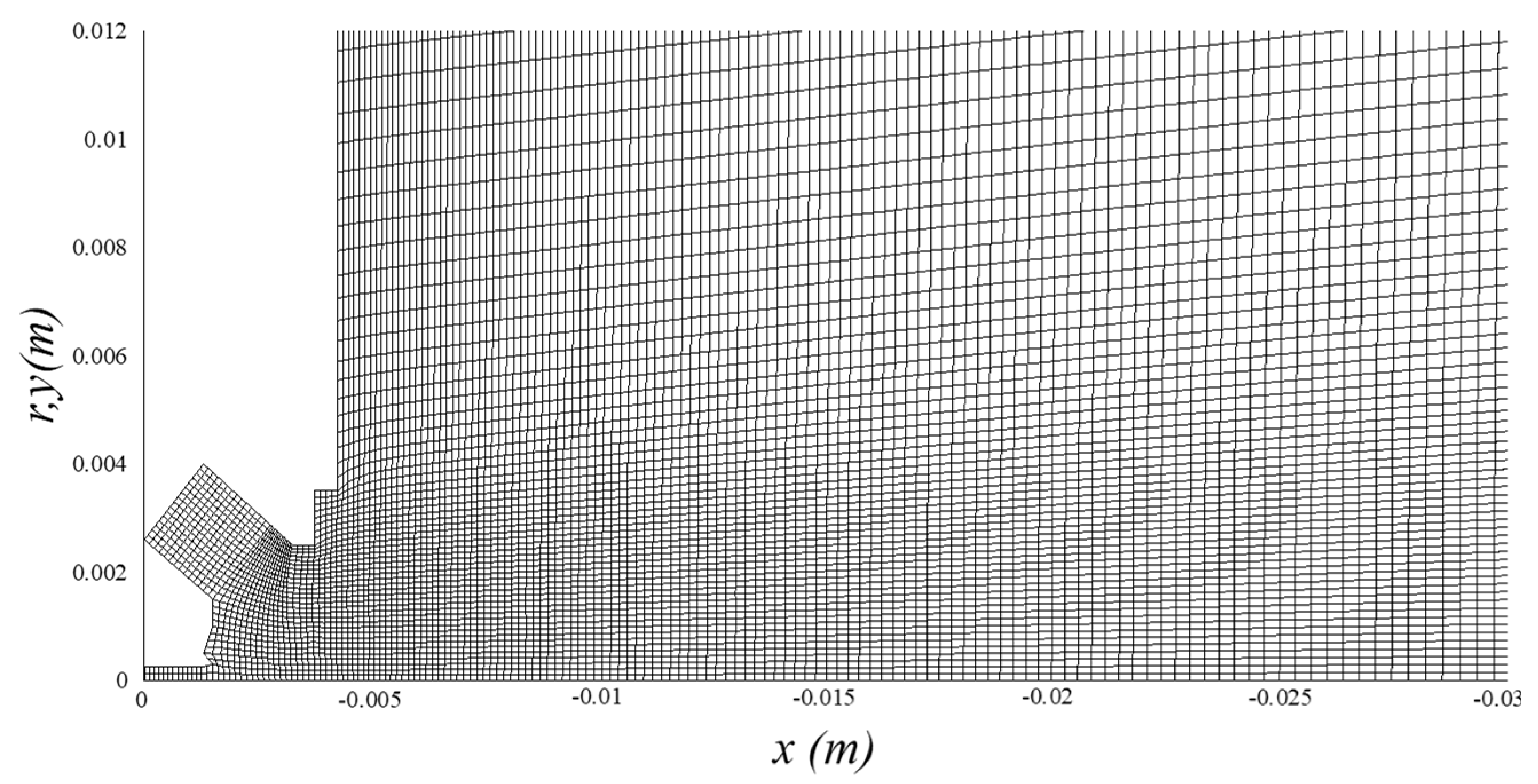
3. Computational Scheme

The full spray simulation program is a modified version of the program used by Kvasnak et al. [8] with the addition of the atomizing air and evaporation model. It is a standalone post-processor code for a given turbulent velocity field. The code uses a Lagrangian approach and solves the equations of motion for solid or liquid ellipsoidal particles undergoing translation, rotation, deformation, breakup and evaporation. The program can also handle the dispersion of a cloud of randomly sized and shaped particles. A semi-implicit backward Euler method is used for the integration of the translational, rotational, and deformation equations for the ellipsoid.
At each time-step, the instantaneous fluid velocity, its first derivative, and the fluid temperature at the location of the particle are evaluated via a Newton’s iteration scheme along with a trilinear interpolation in generalized coordinates in order to provide communication in their block structured mesh algorithm, allowing for the efficient evaluation of the fluid velocity and its derivatives at the centroid of the particle. First, the Newton iteration method is used to find the particle position in grid coordinates. Then, a trilinear interpolation is used to find the fluid velocity, temperature, and velocity gradients at the particle location. Additional details of the trilinear interpolation were discussed by Kvasnak and Ahmadi [25] and Kvasnak et al. [8].

4. Results

In this section, simulation results for a turbulent liquid spray assisted by non-swirling atomizing air are presented and discussed.

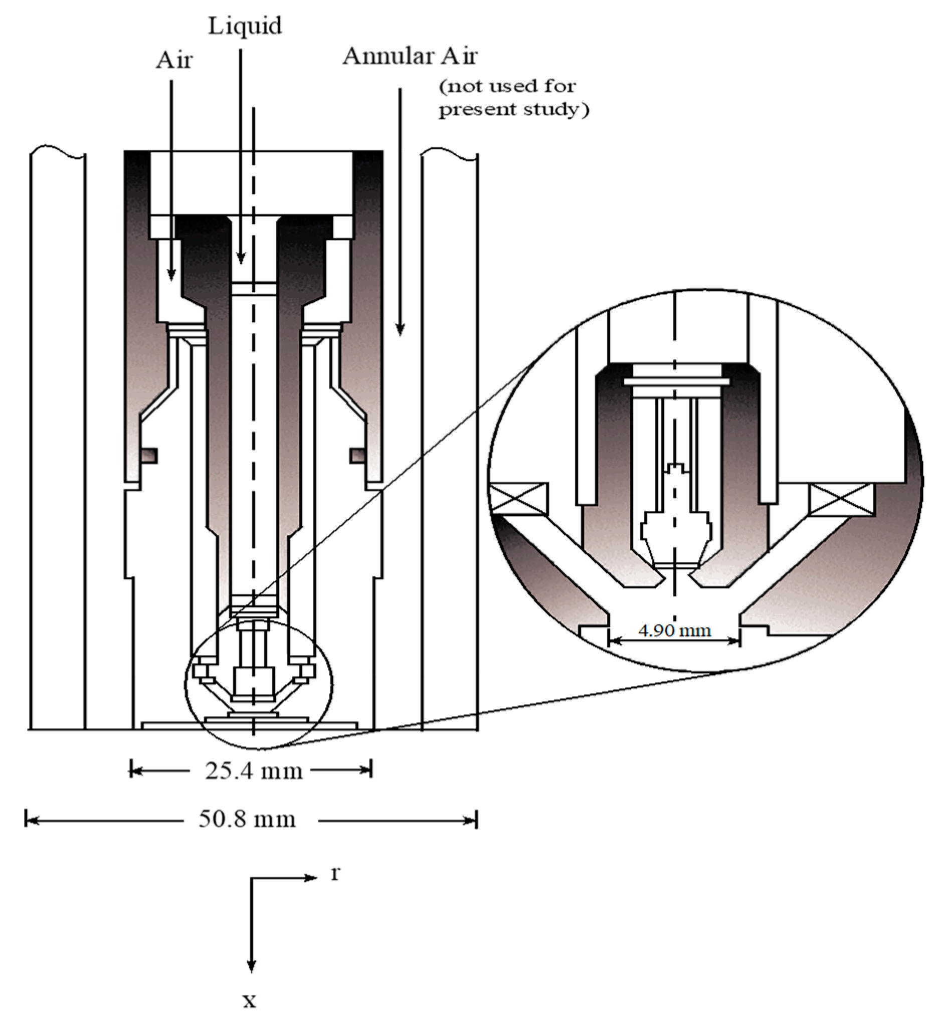
4.1. Simplex Atomizer

The fuel injector used in the present simulation is identical to the one used in the experimental study of McDonell and Samuelsen [22]. In the experiment, a simplex injector tip was mounted centrally within a passage allowing airflow. The geometry of the injector is shown in Figure 4. The simplex tip has a diameter of 0.5 mm and was angled at 41° to the primary direction of flow. In the experiment, the atomizing airflows through a cylindrical cone gap of varying thickness with the gap size of 2.5 mm at the orifice. The fuel spray flowed through a 4.9 mm diameter orifice before issuing into the ambient air. Methanol with a mass flow rate of 1.26 g/s was injected vertically downward as a cone annular sheet. The spray pressure drop was 420 kPa. The atomizing airflow rate was 1.32 g/s with a pressure drop of 3.73 kPa and 13.79 kPa for cases without and with swirling flows, respectively. The experiment was performed at room temperature.
In this study, the experimental conditions of McDonell and Samuelsen [22] with idealized geometry are used and the spray formation from the atomizer is simulated numerically. Liquid methanol is injected as a string of spheres with diameters of 100 μm. The spheres are oriented around the center of the nozzle tip. As they exit through the small orifice at the center of the injector, the particle radial velocity induces the formation of a conical annular sheet. Atomizing air is supplied through the ring surrounding the orifice as an inlet boundary condition.
The fuel injector is simulated using the following steps. The steady state airflow field is first generated using the Reynolds stress transport turbulence model of the ANSYS-FLUENT code. The aspect ratio of the droplet is set to 1.001 and the number of droplets injected is determined by the volume flow rate of liquid through the nozzle. After injection, the droplets are allowed to translate, rotate, deform, breakup, and evaporate in the turbulent gas flow field. Evolution of this process leads to an atomized spray of droplets. As the droplets leave the nozzle, they form a conical annular sheet similar to that observed in the experiment. One major feature of the present simulation is that all of the particles formed by the spray are tracked for their lifetime (i.e., either they evaporate or leave the computational space through an outer boundary surface).
Figure 5 shows a close up of the grid used in the simulation of the simplex atomizer near the injector orifice. The computational space is axisymmetric with a radius of 50 mm and a length of 200 mm. Body-fitted coordinates are used in the computation so that the detailed feature of the atomizer nozzle can be accounted for. A grid sensitivity study was performed using different size meshes. Finally, a grid of 201 by 51 cells that is uniformly expanding in both the streamwise and radial directions is selected and used for the present simulations. A computational grid near the tip of the nozzle is relatively dense to improve the resolution in this critical region. Nevertheless, since the nozzle is very small, only a couple of cells cover the interior of the nozzle. The boundary conditions in the radial direction are symmetry at r = 0 and continuous outflow at r = 50 mm. The boundary conditions in the streamwise direction is no slip wall at x = 0, except for the nozzle inlet which is at a constant velocity and continuous outflow at x = 200 mm. The inlet boundary conditions are uniform velocity equal to that specified in the experiment. For the injector tip here, the inflow boundary condition is 8.35 m/s.

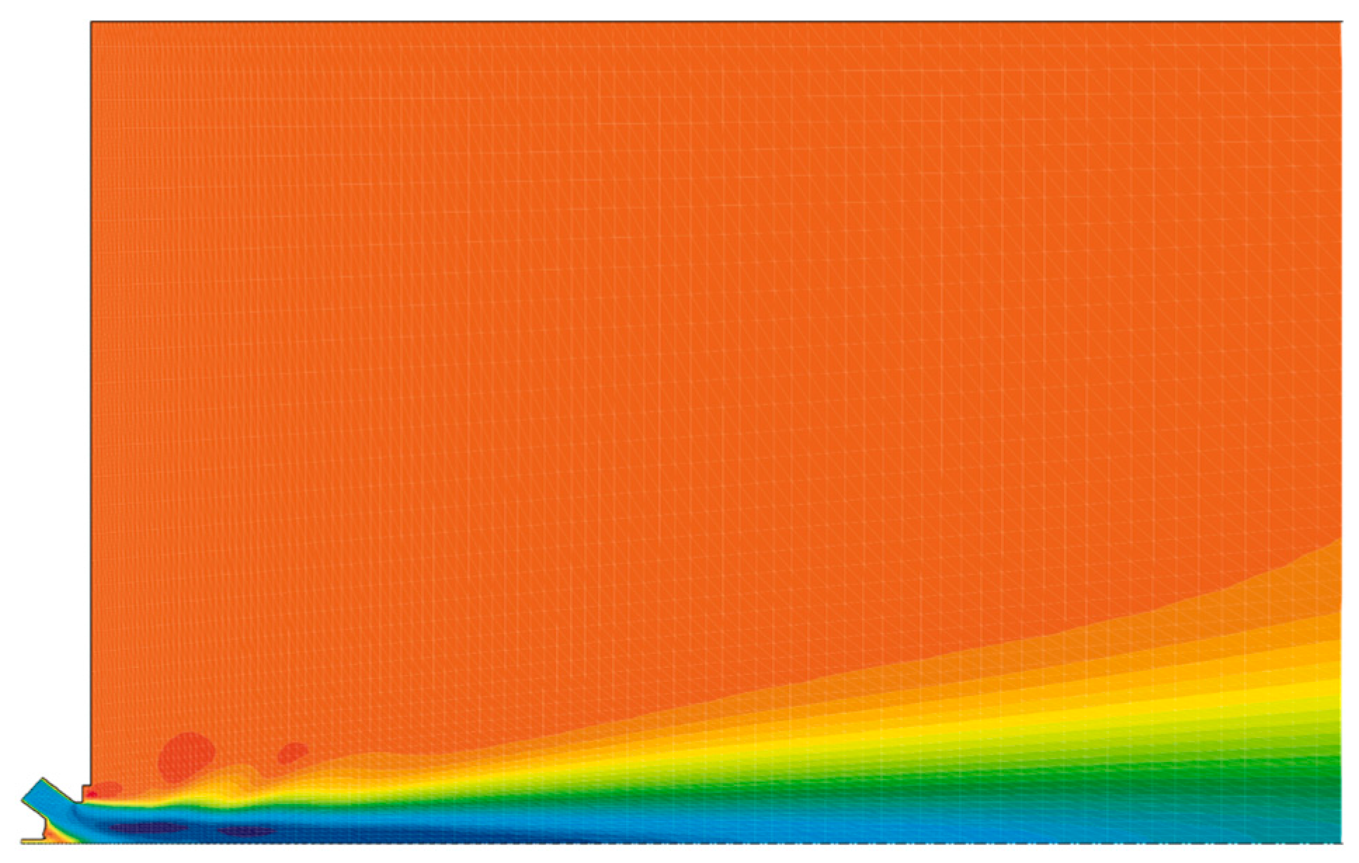
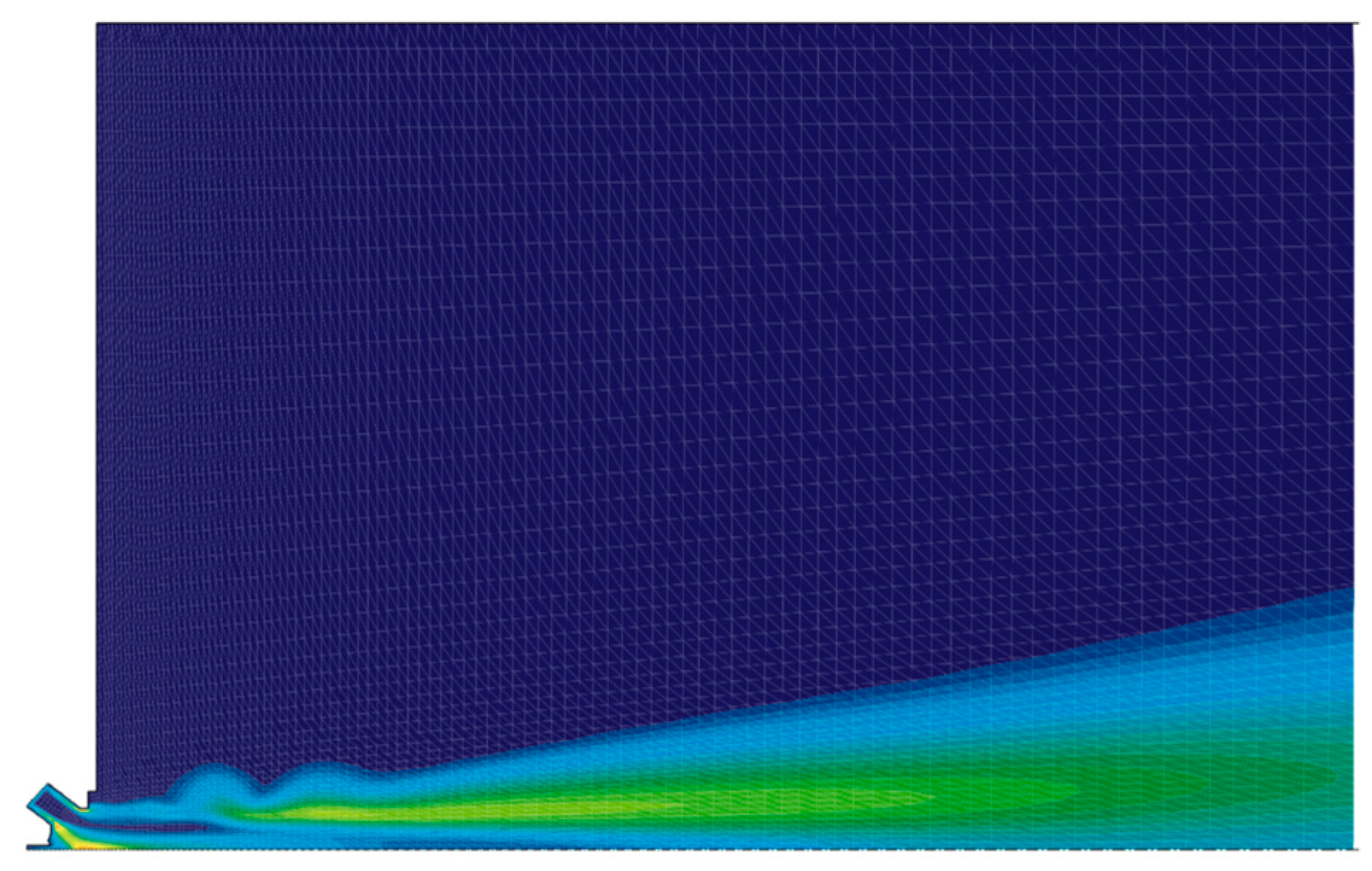
4.2. Non-Swirling Atomizing Air

This section describes the steady state flow field of the injector with non-swirling atomizing air as evaluated by the ANSYS-FLUENT code assuming an inlet velocity of 26.8 m/s.
Figure 6 shows the streamwise velocity contours downstream of the nozzle. This figure clearly shows the development of the shear layer at the edge of the atomizing air jet and the suppression of the shear layers generated by the nozzle flow. As the flow develops the velocity decays in amplitude and spreads radially. A small recirculation region created at the tip of the atomizing air orifice can also be seen in this figure.
Computed contours of turbulence kinetic energy that are shown in Figure 7 indicate the presence of two shear layers which are associated with the nozzle jet or atomizing air. The nozzle jet shear layer diminishes after short distances, while the atomizing air shear layer expands across the region. The peak in the turbulence kinetic energy occurs near the center of the shear layer; however, the kinetic energy is stronger at the point where the annular jet reaches the axis of the injector.
Figure 8 and Figure 9 show the computed contours of components of the Reynolds stress tensor u y 2 ¯ and u x u y ¯ . From Figure 8, it is seen that the peak value of the normal stress u y 2 ¯ occurs near the middle of the shear layer. Figure 9 shows the turbulence shear stress contours, and indicates that the shear stress u x u y ¯ has large values in the downstream vicinity of the nozzle and reaches its peak near the center of the shear layer. These fluctuation flow statistics are used in the Langevin equation model for generating the instantaneous fluid velocity at the location of droplets. The spray formation is described in the subsequent section.

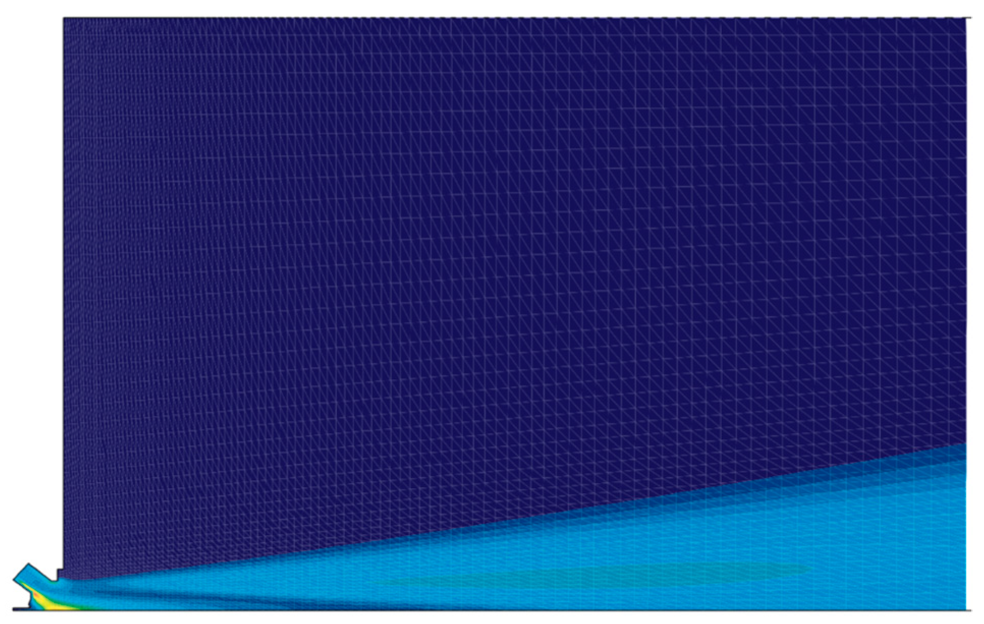
4.3. Spray Simulation

The qualitative comparison of the predicted spray angle in the presence of atomizing air with the experimental data reported by McDonell and Samuelsen [22] is presented in Figure 10. The left-hand side of the figure corresponds to the simulated spray while a picture of the experimental spray is shown on the right side. In this figure, the location and sizes of all droplets in the flow 0.02 s after the spray is turned on are shown. As was noted before, the computational domain is 50 mm wide and 200 mm long. The spray figure is truncated at an axial distance of 100 mm, which is far from the downstream boundary condition. Each initial droplet breaks on the average into four daughter droplets in this flow field through the primary breakup mechanisms. A total of 25,000 droplets are formed in this spray during the period of 0.02 s. Qualitative agreement is seen between the computational spray and the experimental spray with a difference in spray angles of a few percent.
In Figure 11, the radial distance of droplet position downstream of the nozzle exit at axial locations of 25, 50, and 75 mm are shown. At 25 mm downstream, the spray is an annular cone with a thickness of approximately 2 mm, and the radial distribution function is symmetric with a very small standard deviation. Further downstream at 50 mm, the spray is still an annular cone and has a thickness of approximately 5 mm with no droplets in the core region. The distribution function is also roughly symmetric across the spray region. Further downstream at 75 mm, the spray is still an annular cone with a thickness of approximately 15 mm. The distribution function is skewed with its peak moving toward the outer edge of the spray cone and a longer tail toward the inner cone.
Figure 12 shows the variation of the droplet minimum diameter at axial distances of 25, 50, and 75 mm downstream of the nozzle exit. At a downstream position of 25 mm, the droplet minimum diameter is in the range of 30 μm to 40 μm, with the central part of the spray cone containing slightly larger sizes compared to the edges. At 50 mm downstream, the droplet minimum diameter is scattered in range of 40 μm to 60 μm with the mean of about 50 μm. While at 75 mm downstream, the droplet minimum diameter varies more narrowly between 70 μm to 80 μm with a mean of about 75 μm.
Figure 13 shows the predicted droplet aspect ratio at downstream axial positions of 25, 50, and 75 mm. It is observed that the droplets at the distance of 25mm are highly elongated having aspect ratios observed between 11 and 13 with the highest values appearing on the edges of the spray. At a downstream position of 50 mm, the droplets are still quite elongated with aspect ratios ranging from 6 to 11. Further downstream at axial distance of 75 mm from the injector, the droplets become nearly spherical with some having aspect ratios about 1.5 to 2. It can be seen that the droplets deform significantly between the axial distances of 25 and 50 mm and particularly from 50 to 75 mm. The reason is that the velocity gradient decrease with distance from the spray nozzle and becomes quite small at the axial distance of about 75 mm. In the absence of shear induced deformation, the droplets tend to become spherical under the action of surface tension.
Figure 14 compares the predicted Sauter mean diameters at distances of 25, 50, and 75 mm downstream from the injector with the experimental data of McDonell and Samuelsen [22]. Here, for the model predictions, the Sauter mean diameter of the equivalent volume spherical droplet is used for non-spherical droplets. The simulated droplets have a roughly constant Sauter diameter of about 75 μm to 80 μm, while the experimental data show a Sauter diameter of about 50 μm to 65 μm at the axial distance of 25 mm, and a diameter in the range of 50 μm to 70 μm at a distance of 50 and 75 mm. The experimental data show a continuous decrease of diameter toward the centerline, and the presence of small droplets in the core region. The simulation, however, predicts no droplets in the core region. It is conjectured that the smaller droplet size in the experiment and the presence of very small droplets in the core is due to the secondary breakup mechanisms. In the present study, the secondary break was not included in the computational model as the bulk of the mass of the spray is accounted for by the primary breakup mechanism. The absence of the secondary breakup in the model is perhaps the main cause for the discrepancy seen in Figure 14 for smaller particles. In addition, it should be pointed out that the present model prediction suggests that the droplets are highly elongated at short distances from the nozzle and this could introduce error in the experimental Phase Doppler Anemometry (PDA) measurements.
Further downstream, the variations of the Sauter diameter are similar to that shown for 25 mm downstream except for the spreading of the spray to larger radial segment. As noted before, the simulated D32 overestimates the experimental data by approximately 15–20%. In addition, the simulation also did not capture the smaller droplets in the central region of the annular cone that are generated by the secondary breakup.
Figure 15 compares the predicted streamwise droplet velocity, ux, with the experimental data of McDonell and Samuelsen [22] at 25, 50, and 75 mm downstream of the nozzle. The flow velocity profiles as predicted by the ANSYS-FLUENT code are shown by solid lines in the figure for comparison. The predicted and experimental droplet velocities are larger than the flow velocities. The experimental data of McDonell and Samuelsen [22], however, show a sharp increase in velocity toward the centerline. As noted before, in this region, the droplets are smaller and are generated by the secondary breakup mechanism. The predicted particle velocities are shown only for the range of spray layer as there are no particles in the core region. As was mentioned before, the present computational model for spray formation lacks the secondary breakup mechanisms and, therefore, the formation small particles are missed.
Figure 15 also shows that the simulated droplet velocity across the spray in the region 10 r 15 mm at axial distance of 25 mm is in reasonable agreement with the experimental data. Similarly, the predicted velocity at distance of 50 and 75 mm are comparable with the experimental data for the range that the simulations results are available.

5. Conclusions

In this work, the formation of a spray in a fuel injector with atomizing airflow field is studied. The equations of motion for the translation and rotation of an ellipsoidal droplet are presented. The evaporation rate of a non-spherical droplet is included. Physical models for the deformation and breakup of liquid droplets in the presence of shear flow and pressure gradient fields are described. A Langevin equation for generating instantaneous air velocities that satisfy the Navier–Stokes approximately (via a closed PDF formulation) is used for evaluating the droplet trajectories. In addition, a novel application of the Newton iteration and trilinear interpolation in generalized coordinates is used as the basis for the spray simulation algorithm, in which every droplet is traced through the flow field. The general conclusions of the study are:
  • The presented engineering model for simulation of spray leads to results that are in qualitative agreement with the experimental data for the studied cases.
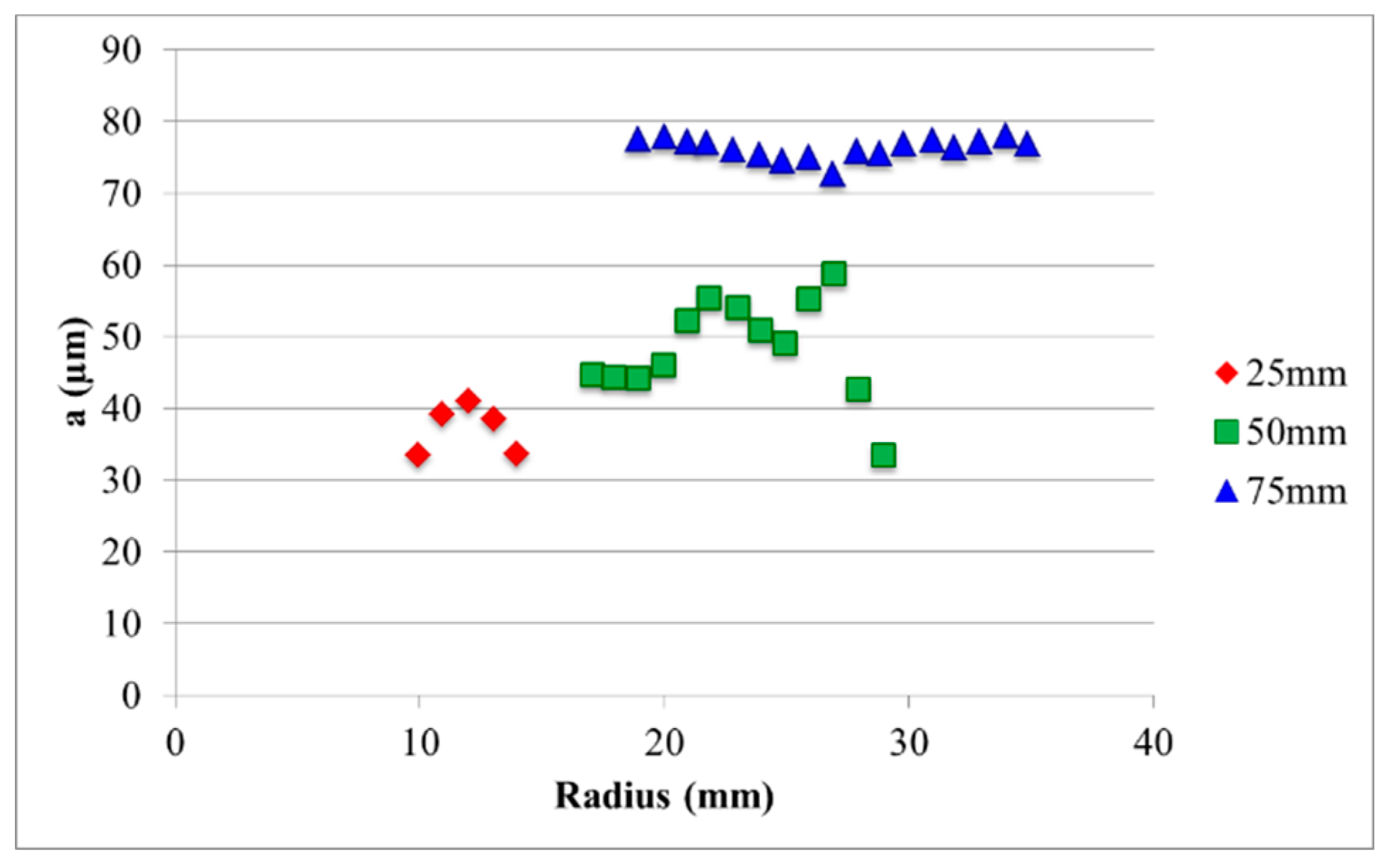
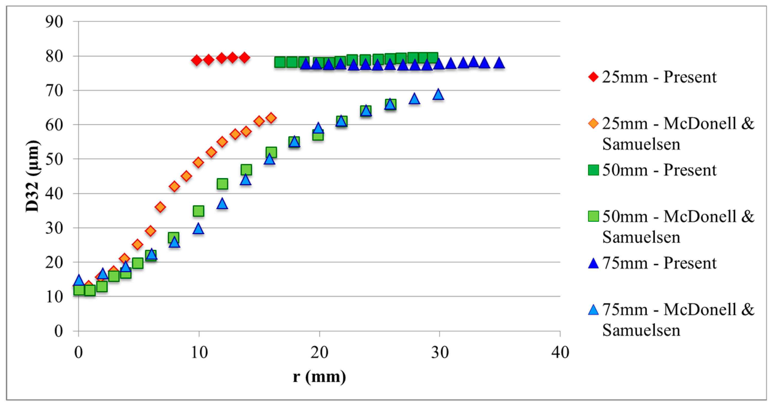
  • The average droplet size due to primary breakup mechanisms is in good agreement with the experimental data in regions of the flow where the droplets are nearly spherical.
  • In regions of the spray where the droplets are elongated, the predicted droplet diameter overestimates the experimental data.
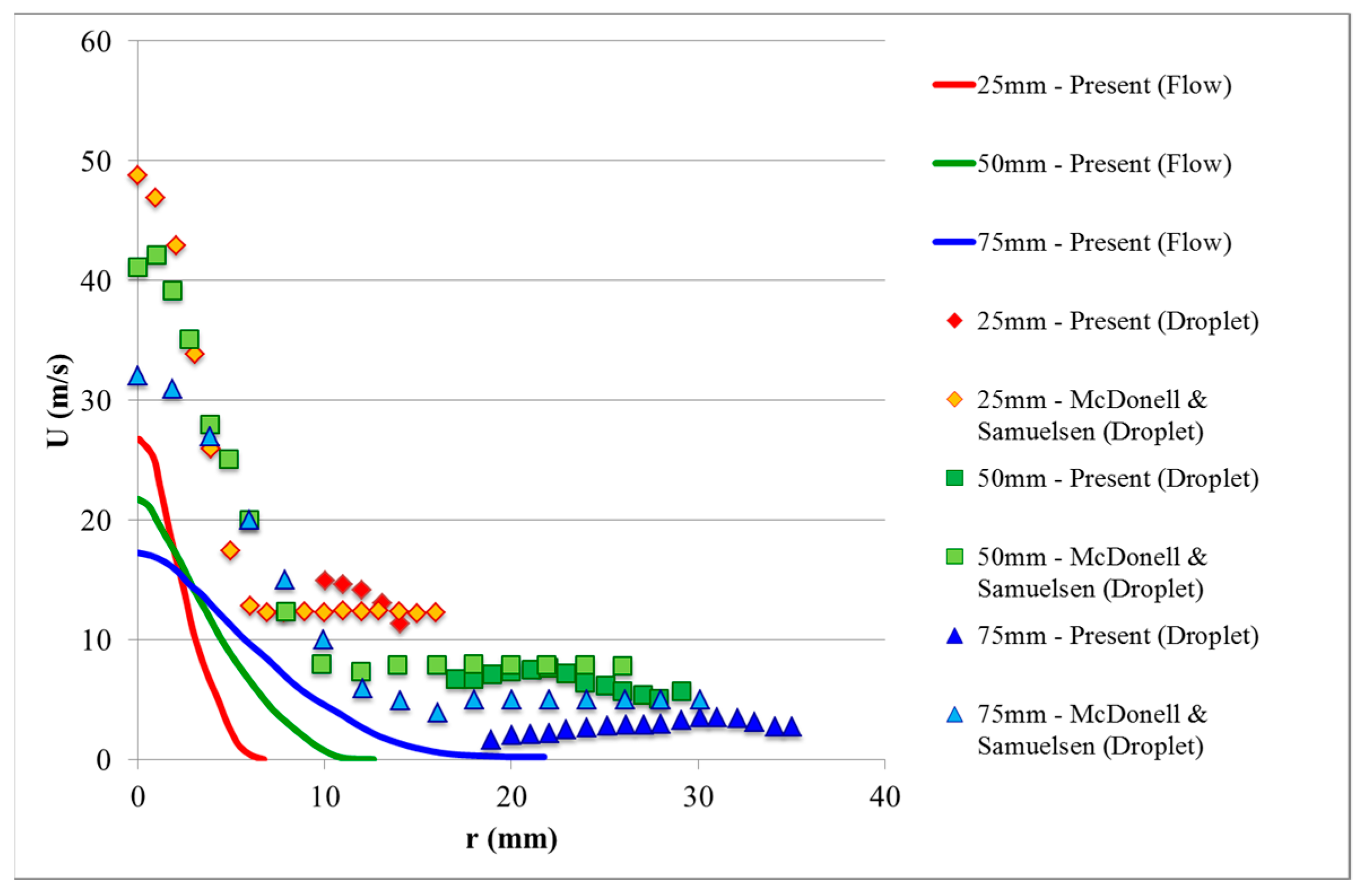
  • The droplet velocity is in reasonable agreement with the experimental data.
  • Droplet aspect ratio affects the evaporation rate of droplets.
  • Evaporation affects the fluctuation velocity of droplets, but it has little effect on the droplet diffusivity.
  • The presented model and simulation algorithm provides a viable tool for the computational prediction of spray simulations.
  • Secondary breakup mechanisms may play a major role in the atomization of sprays with complex atomizing airflow patterns and must be included in future studies.

Author Contributions

This study was a part of the PhD research works of D.J.S. and W.K. who was responsible for developing the computational model and for performing the simulations and data analysis. G.A. contributed to the interpretation of the results and to the critical revision of the article.

Funding

The earlier part of this research was funded by NASA-Marshall under Grant No. NGT-51130.

Acknowledgments

The authors would like to thank Charles Schafer and George Schmidt of NASA Marshall for many valuable discussions and constructive comments. Fa-gung Fan is also acknowledged for many helpful discussions. The financial support of NASA-Marshall Space Flight Center for the earlier part of this effort is gratefully acknowledged.

Conflicts of Interest

The authors declare no conflict of interest.

References

  1. Faeth, G. Evaporation and combustion of sprays. Prog. Energy Combust. Sci. 1983, 9, 1–76. [Google Scholar] [CrossRef]
  2. Law, C. Recent advances in droplet vaporization and combustion. Prog. Energy Combust. Sci. 1982, 8, 171–201. [Google Scholar] [CrossRef]
  3. Jiang, X.; Siamas, G.; Jagus, K.; Karyiannis, T. Physical modelling and advanced simulations of gas-liquid two-phase jet flows in atomization and sprays. Prog. Energy Combust. Sci. 2010, 36, 131–167. [Google Scholar] [CrossRef]
  4. Gutheil, E. Issues in computational studies of turbulent spray combustion. In Experiments and Numerical Simulations of Diluted Spray Turbulent Combustion; Merci, B., Roekaerts, D., Sadiki, A., Eds.; Springer: Berlin, Germany, 2011. [Google Scholar]
  5. Jenny, P.; Roekaerts, D.; Beishuizen, N. Modeling of turbulent dilute spray combustion. Prog. Energy Combust. Sci. 2012, 38, 846–887. [Google Scholar] [CrossRef]
  6. Shang, H.M.; Chen, C.P.; Jiang, Y. Turbulence Modulation Effect on Evaporating Spray Characterization. In Proceedings of the 26th Joint Propulsion Conference, Orlando, FL, USA, 16–18 July 1990. [Google Scholar]
  7. Berlemont, A.; Grancher, M.-S.; Gouesbet, G. On the Lagrangian Simulation of Turbulence Influence on Droplet Evaporation. Int. J. Heat Mass Transf. 1991, 34, 2805–2812. [Google Scholar] [CrossRef]
  8. Kvasnak, W.; Ahmadi, G.; Schmidt, D.J. An Engineering Model for the Fuel Spray Formation of Deforming Droplets. At. Sprays 2004, 14, 289–339. [Google Scholar] [CrossRef]
  9. Kolakaluri, R.; Li, Y.; Kong, S.-C. A unified spray model for engine spray simulation using dynamic mesh refinement. Int. J. Multiph. Flow 2010, 36, 858–869. [Google Scholar] [CrossRef]
  10. Keller, J.; Gebretsadik, M.; Habisreuther, P.; Turrini, F.; Zarzalis, N.; Trimis, D. Numerical and experimental investigation on droplet dynamics and dispersion of a jet engine injector. Int. J. Multiph. Flow 2015, 75, 144–162. [Google Scholar] [CrossRef]
  11. Doisneau, F.; Arienti, M.; Oefelein, J.C. A semi-Lagrangian transport method for kinetic problems with application to dense-to-dilute polydisperse reacting spray flows. J. Comput. Phys. 2017, 329, 48–72. [Google Scholar] [CrossRef]
  12. Hoyas, S.; Gil, A.; Margot, X.; Khuong-Anh, D.; Ravet, F. Evaluation of the Eulerian-Lagrangian Spray Atomization (ELSA) model in spray simulations: 2D cases. Math. Comput. Model. 2013, 57, 1686–1693. [Google Scholar] [CrossRef]
  13. Apte, S.V.; Gorokhovski, M.; Moin, P. LES of atomizing spray with stochastic modelling of secondary breakup. Int. J. Multiph. Flow 2003, 29, 1503–1522. [Google Scholar] [CrossRef]
  14. Jones, W.P.; Lettieri, C. Large eddy simulation of spray atomization with stochastic modelling of breakup. Phys. Fluids 2010, 22, 115106. [Google Scholar] [CrossRef]
  15. Irannejad, A.; Banaeizadeh, A.; Jaberi, F. Large eddy simulation of turbulent spray combustion. Combust. Flame 2015, 162, 431–450. [Google Scholar] [CrossRef]
  16. Jones, W.P.; Marquis, A.J.; Noh, D. An investigation of a turbulent spray flame using Large Eddy Simulation with a stochastic breakup model. Combust. Flame 2017, 186, 277–298. [Google Scholar] [CrossRef]
  17. Khan, M.M.; Hélie, J.; Gorokhovski, M. Computational methodology for non-evaporating spray in quiescent chamber using Large Eddy Simulation. Int. J. Multiph. Flow 2018, 102, 102–118. [Google Scholar] [CrossRef]
  18. Noh, D.; Gallot-Lavallée, S.; Jones, W.P.; Navarro-Martinez, S. Comparison of droplet evaporation models for a turbulent, non-swirling jet flame with a polydisperse droplet distribution. Combust. Flame 2018, 194, 135–151. [Google Scholar] [CrossRef]
  19. Li, K.; Zhou, L.X.; Chan, C.K.; Wang, H.G. Large-eddy simulation of ethanol spray combustion using a SOM combustion model and its experimental validation. Appl. Math. Model. 2015, 39, 36–49. [Google Scholar] [CrossRef]
  20. Senoner, J.M.; Sanjose, M.; Lederlin, T.; Faegle, F.; Garcia, M.; Riber, E.; Cuenot, B.; Gicquel, L.; Pitsch, H.; Poinsot, T. Eulerian and Lagrangian Large-Eddy Simulations of an Evaporating Two-phase Flow. C. R. Mecanique 2009, 337, 458–468. [Google Scholar] [CrossRef]
  21. Prasad, V.N.; Masri, A.R.; Navarro-Martinez, S.; Luo, K.H. Investigation of auto-ignition in turbulent methanol spray flames using Large Eddy Simulation. Combust. Flame 2013, 160, 2941–2954. [Google Scholar] [CrossRef]
  22. McDonell, V.G.; Samuelsen, G.S. An Experimental Data Base for the Computational Fluid Dynamics of Reacting and Nonreacting Methanol Sprays. J. Fluids Eng. 1995, 117, 145–153. [Google Scholar] [CrossRef]
  23. O’Rourke, P.J.; Amsden, A.A. The TAB Method for Numerical Computation of Spray Droplet Breakup. SAE Tech. Paper 872089. Available online: https://www.sae.org/publications/technical-papers/content/872089/ (accessed on 20 January 2019).
  24. Ibrahim, F.A.; Yang, H.Q.; Przekwas, A.J. Modeling of Spray Droplets Deformation and Breakup. AIAA J. Propuls. 1993, 9, 651–654. [Google Scholar] [CrossRef]
  25. Kvasnak, W.; Ahmadi, G. Computational Modeling of Dispersion of Deforming Fuel Droplets in a Spray Injector Flow Field. In Proceedings of the 1996 Joint Army-Navy-NASA-Air Force (JANNAF) Propulsion Meeting, JPM and JSM 96, Albuquerque, NM, USA, 9–13 December 1996. [Google Scholar]
  26. Fan, F.-G.; Ahmadi, G. Dispersion of Ellipsoidal Particles in an Isotropic Pseudo-Turbulent Field. ASME J. Fluids Eng. 1995, 117, 154–161. [Google Scholar] [CrossRef]
  27. Zhang, H.; Ahmadi, G.; Fan, F.-G.; Mclaughlin, J.B. Ellipsoidal particles transport and deposition in turbulent channel flows. Int. J. Multiph. Flow 2001, 27, 971–1009. [Google Scholar] [CrossRef]
  28. Goldstein, H. Classical Mechanics, 2nd ed.; Addison-Wesley: Boston, MA, USA, 1980. [Google Scholar]
  29. Gallily, I.; Cohen, A.H. On the Orderly Nature of the Motion of Nonspherical Large Droplet and Axially Symmetrical Elongated Particles. J. Colloid Interface Sci. 1979, 68, 338–356. [Google Scholar] [CrossRef]
  30. Hughes, P.C. Spacecraft Attitude Dynamics; John Wiley and Sons: New York, NY, USA, 1986. [Google Scholar]
  31. Happel, J.; Brenner, H. Low Reynolds Number Hydrodynamics; Springer Science and Business Media: Berlin, Germany, 1973. [Google Scholar]
  32. Harper, E.Y.; Chang, I.-D. Maximum dissipation resulting from lift in a slow viscous shear flow. J. Fluid Mech. 1968, 33, 209–225. [Google Scholar] [CrossRef]
  33. Jeffery, G.B. The Motion of Ellipsoidal Particles Immersed in a Viscous Fluid. Proc. R. Soc. Lond. A 1922, 102, 161–179. [Google Scholar] [CrossRef]
  34. Stone, H.A. Dynamics of Drop Deformation and Breakup in Viscous Fluids. Ann. Rev. Fluid Mech. 1994, 26, 65–102. [Google Scholar] [CrossRef]
  35. Haworth, D.C.; Pope, S.B. A generalized Langevin model for turbulent flows. Phys. Fluids 1986, 29, 387–405. [Google Scholar] [CrossRef]
  36. Haworth, D.C.; Pope, S.B. A pdf modeling study of self-similar turbulent free shear flows. Phys. Fluids 1987, 30, 1026–1044. [Google Scholar] [CrossRef]
  37. Girimaji, S.S.; Pope, S.B. A diffusion model for velocity gradients in turbulence. Phys. Fluids 1990, 2, 242–256. [Google Scholar] [CrossRef]
Figure 1. Coordinate system.
Fluids 04 00020 g001
Figure 2. Euler parameters.
Fluids 04 00020 g002
Figure 3. Drag coefficient correction (Equation (20)) in the (a) x ^ , z ^ directions; (b) y ^ -directon.
Fluids 04 00020 g003
Figure 4. Geometry of the Simplex atomizer.
Fluids 04 00020 g004
Figure 5. Close-up view of the computational grid of the Simplex atomizer.
Fluids 04 00020 g005
Figure 6. Streamwise velocity with non-swirling atomizing air.
Fluids 04 00020 g006
Figure 7. Turbulent kinetic energy of the flow with non-swirling atomizing air.
Fluids 04 00020 g007
Figure 8. u y 2 ¯ of the flow with non-swirling atomizing air.
Fluids 04 00020 g008
Figure 9. u x u y ¯ of the flow with non-swirling atomizing air.
Fluids 04 00020 g009
Figure 10. Qualitative comparison of spray angle with non-swirling atomizing air.
Fluids 04 00020 g010
Figure 11. Radial distribution of droplet position at 25, 50, and 75 mm with non-swirling atomizing air.
Fluids 04 00020 g011
Figure 12. Droplet minimum diameter at axial distances of 25, 50, and 75 mm with non-swirling atomizing air.
Fluids 04 00020 g012
Figure 13. Droplet aspect ratio at axial distances of 25, 50, and 75 mm with non-swirling atomizing air.
Fluids 04 00020 g013
Figure 14. Sauter mean diameter of droplets at axial distances of 25, 50, and 75 mm with non-swirling atomizing air.
Fluids 04 00020 g014
Figure 15. Axial velocity of droplets at axial distances of 25, 50, and 75 mm with non-swirling atomizing air.
Fluids 04 00020 g015

