Abstract
Analytic formulations of elementary flow field profiles in weakly anisotropic nematic fluid are determined, which can be attributed to biological or artificial micro-swimmers, including Stokeslet, stresslet, rotlet and source flows. Stokes equation for a nematic stress tensor is written with the Green function and solved in the k-space for anisotropic Leslie viscosity coefficients under the limit of leading isotropic viscosity coefficient. Analytical expressions for the Green function are obtained that are used to compute the flow of monopole or dipole swimmers at various alignments of the swimmers with respect to the homogeneous director field. Flow profile is also solved for the flow sources/sinks and source dipoles showing clear emergence of anisotropy in the magnitude of flow profile as the result of fluid anisotropic viscosity. The range of validity of the presented analytical solutions is explored, as compared to exact numerical solutions of the Stokes equation. This work is a contribution towards understanding elementary flow motifs and profiles in fluid environments that are distinctly affected by anisotropic viscosity, offering analytic insight, which could be of relevance to a range of systems from microswimmers, active matter to microfluidics.
1. Introduction
Microswimmers are biological or artificial entities that are characterized by locomotion at microscopic scales, such as bacteria, protozoa, spermatozoa, algae, or Janus colloids, self-propelling droplets, shape-shifting swimmers, and rotating colloids [1,2,3]. The locomotion of the swimmers is affected by their relatively small size (order of magnitude ) and relatively slow propulsion (up to few ) [1,3], which determines that their dynamics is described by the Stokes equation (rather than the full Navier–Stokes), as having very small Reynolds numbers (). As recognized by Purcell, the swimming mechanism of such microswimmers requires swimming strokes that are irreversible in time [4]. While swimming of biological microswimmers is an essential part of their survival and reproduction, artificial microswimmers not only help to understand the biomechanics behind swimming organisms [5], but could possibly be also utilized to drive gears (produce work) [6,7], enhance the diffusion of a solution [8], increase stirring by the process of particle entrainment [9] or produce frictionless fluids [10,11].
Microswimmers are often faced with non-Newtonian environment. For example, biological fluids, such as blood, mucus, and saliva show viscoelastic behavior [12], and cytoskeleton of animal cells shows orientational order [13]. Furthermore, many biomaterials can form a nematic phase [14]. To investigate the influence of anisotropic background on swimming bacteria, studies of bacterial solutions in lyotropic liquid crystals were conducted, investigating the behavior of single bacteria [15,16,17], their pairwise interaction [18] or their collective motion [19,20]. Bacterial suspensions in liquid crystals can be used for transport of microcargo [21]. While investigating swimming bacteria in liquid crystals is particularly challenging due to high toxicity of many nematics, this problem is avoided by studying artificial active particles in liquid crystals [22], or, for example, properties of a Taylor’s swimming sheet [23,24]. Even passive systems, such as sedimentation of spheres shows an intertwined behavior of fluid velocity and internal structure of nematics. Flow profiles in a nematic liquid crystal were discussed typically in the context of a moving sphere inside a nematic for a case of homogeneous [25,26] or inhomogeneous [27,28,29] director profile. In [30], the solution for the flow profile and the drag force on a moving sphere were determined in the weakly anisotropic limit. In [31], the problem of nematic flow around a sphere was investigated by the use of Green functions for the Stokes equation, which is a method that is applied also in this article. Biological and artificial swimmers in non-Newtonian fluids, possibly with a anisotropic structure, represent a further complexity in their underlying physics. Finally, understanding the effects of the internal structure of the complex fluids on the microswimmers is an open challenge in both living systems as well as designed devices.
The flow fields caused by the microswimmers can be characterized by the moments of force that microswimmers apply on a fluid [1,2,3]. If a microswimmer exerts an effective point force on a fluid, we speak of a Stokeslet flow. Such flows have been observed in the case of Volvox carteri [32] and externally driven colloids [5]. A microswimmer that exerts an effective force dipole on a fluid produces a stresslet or rotlet flow. Stresslet is a typical flow profile for swimming microorganisms, such as Escherichia coli [33] or self-driven colloids [5]. Although multipolar approach ignores the details of the flow field close to the swimmers, for example around the flagella, its particular advantage is that higher order multipoles decay faster with the distance from the swimmer. Therefore, it is especially efficient in semi-dilute suspensions, where multipolar expansion of the flow field was used to investigate problems such as fluid mixing by the microswimmers [34], interaction between microswimmers [35,36], and collective behaviour in microswimmer suspensions [37,38]. The swimmer flow field can be additionally affected by the confinement, as, for example, in thin films [39] or droplets [40], where the orientation and position of the swimmer with respect to the boundary determines the flow field and the behavior of microswimmers. In dense suspensions, the dominating interactions are steric, electrostatic, van der Waals and close-field hydrodynamic [3]. In such high-density suspensions, swimmers tend to move in swarms, or can even produce an active nematic phase [41].
In this paper, we determine the analytical formula for flow fields of micro-swimmers—represented as point forces, point torques, or stresslets—in anisotropic nematic fluids, under the assumption of uniform nematic alignment and within the first order expansion of the anisotropy of the viscosity tensor. Specifically, we first calculate analytical approximations of the Green function to the Stokes equation with anisotropic viscosity, included via the nematic-type stress formulation, and then use these solutions to construct the flow fields of point force, point torque, and stresslet in uniform nematic fluid. Using a similar approach, we also determine analytically the flow field of point sinks and sources in a uniform nematic. Distinctly, we show how the direction of the applied forces and torques with respect to the nematic director affects the calculated flow profiles. The two key assumptions of the demonstrated analytical solutions—uniformity of nematic field and anisotropy expansion in viscosity—are discussed. Anisotropy expansion in viscosity is tested against precise numerical solutions. More generally, the results of this paper give analytical insight into elementary flow field profiles applicable to micro-swimmers in anisotropic fluids and could be used to further explore more complicated flow profiles and swimming dynamics in various complex environments.
2. Results
2.1. Nematic Green Function for the Stokes Equation
A strong approach to the formulation of elementary flow profiles as generated by local stimuli—like micro-swimmers—is to first consider point-like forces acting on a fluid, which is known as the Method of Green’s functions [42]. Specifically, in a distinct point in space, a point force is taken to act on the fluid (in our case at ), and then one tries to solve the corresponding flow field from the dynamic equation of the fluid. For fluid flows relevant to micro-swimmers, we are interested in the solutions of the Stokes equation with a point force acting on a fluid:
where is a spatial derivative along the i-th direction, p is the fluid pressure, a point force, the stress tensor, and the three-dimensional Dirac delta function. We also assume incompressible flow . Equation (1) needs to be solved for both the pressure field and the velocity field . The solution of Equation (1) is called Stokeslet and is well known for isotropic fluids [42], where the stress tensor is proportional to the strain rate (Figure 1). Often, the interaction between a microswimmer and the surrounding fluid is not best described by a single point force, but by a distribution of forces. In this case, the main advantage of the Green function approach is that, once the solution for the point force is found, it can be easily expanded to other force distribution, such as a pair of opposite forces (stresslet flow), or a point torque (rotlet flow), solutions which are shown in Figure 1 for the isotropic stress tensor. Here, we are interested in the same elementary solutions, however in the systems with the nematic degree of order, i.e., with anisotropic viscosity and some preferred homogeneous orientation (director) field of the system. The anisotropy of the system is reflected in the nematic stress tensor, which we write in the Ericksen–Leslie formulation [43]:
where , , , is the director, the flow field velocity vector, and are six Leslie viscosity coefficients (five are independent due to constraint ). In an isotropic liquid, only viscosity coefficient is non-zero, giving the standard isotropic fluid stress tensor.
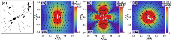
Figure 1.
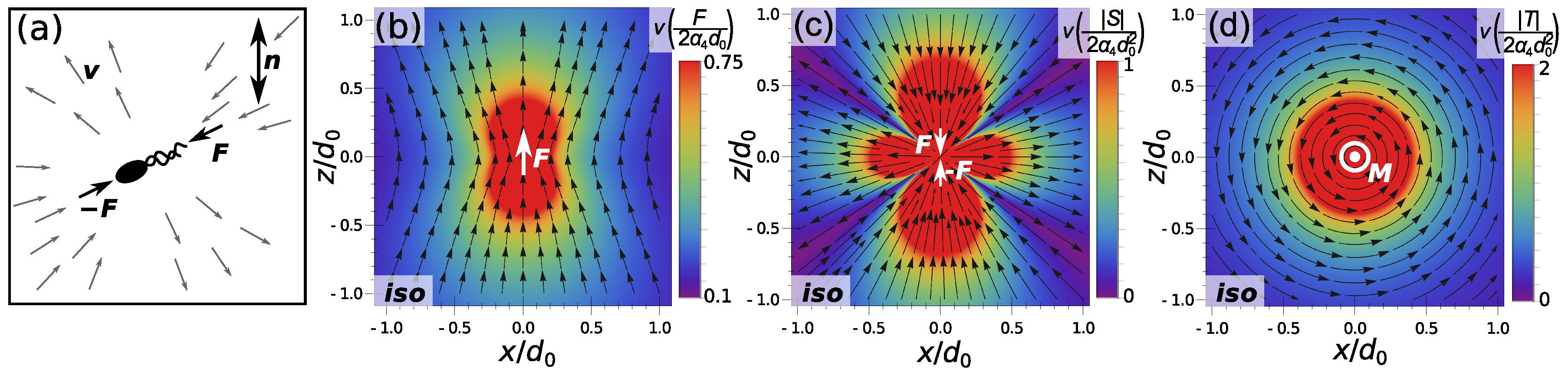
(a) an outline of the problem—a microswimmer exerts forces upon the surrounding nematic fluid with homogeneous director , driving a flow field . A set of elementary flow profile solutions for isotropic fluids is shown as reference for later comparison: (b) Stokeslet flow due to a point force; (c) stresslet flow due to a pair of opposite forces (a force dipole), and (d) rotlet flow due to a point torque. The magnitude of the flow field as noted in the colorbar is given in basic quantities (see text for more).
Flow fields may cause realignment in the nematic orientational profile. The dynamics of the director profile as coupled to the velocity field is given by the equation [43]
where f is a free energy density of the nematic due to elastic deformations of the director field and due to coupling to the external fields, and is a Lagrange multiplier preserving the unit length of . In principle, a solution to the proposed problem of microswimmer flow profiles in nematic fluids could be found by solving the Stokes equation together with the incompressibility condition, and molecular field equation as a set of coupled nonlinear differential equations. Indeed, such solutions could be found by using numerical simulations [44,45], but not analytically. However, a particular question we want to address in this paper is whether some analytic insight can be found, which is quite rare in complex fluid systems. We search for a solution by assuming a homogeneous director field, therefore excluding Equation (3) from our calculations. Such analytic solutions typically prove distinct relevance as they can be used in a variety of experimental or computer modelling setups either for analysis or as elementary building solutions in a much more complex system. For example, one idea would be to take these elementary analytic solutions of individual flow elements and incorporate them as simplest-order approximations in systems of multiple flow objects—like colonies of swimmers.
The posed problem of elementary solutions in Stokes fluid with anisotropic viscosity can be solved analytically—within approximation—if considering the regimes of the anisotropic viscosity coefficients . The large variety of nematic materials—for example from molecular to virus and colloidal, thermotropic or lyotropic, passive or active—exhibit a variety of regimes of the actual values of the viscosity coefficients . For example, in some lyotropic nematics, can be very large, whereas , , , and are smaller in size and , , and are negative [46,47,48]. Differently, in a standard thermotropic nematic like 5 4-cyano-4’-pentylbiphenyl (5CB) , , are of similar order of magnitude which is slightly larger than the magnitude of , whereas and are smaller [49]. However, a common trend in nematic systems is that if the nematic degree of order gets smaller (for example, as when approaching the nematic-isotropic phase transition), the (isotropic) viscosity coefficient typically can become the leading viscosity coefficient [50]. Stimulated by this behaviour of , we assume in this work that is the largest coefficient and calculate the solutions to the Stokes equation that are of first order in other viscosity coefficients. From a more theoretical perspective, such approach of taking isotropic viscosity coefficient as the leading term in the stress tensor can be seen also as searching for solutions that are close to the isotropic fluid solutions but adapted (within first order) for anisotropic viscosity. An example of how to give physical meaning to viscosity coefficients is to compare effective viscosity at different orientations of velocity, velocity gradient, and director field—in the context of Miesowicz geometry [43]. For the hierarchy of , , , and of lyotropic nematics discussed above, the lowest effective viscosity is in the case of a director being parallel to flow direction and perpendicular to flow gradient, whereas the highest viscosity is for a director parallel to flow gradient and perpendicular to flow direction. This regime of viscosity coefficients is used also for the graphic representation of the results throughout the paper, where we use values , , although the calculations are for general values , as long as is the leading viscosity coefficient.
We solve the Stokes equation (Equation (2)) with the assumption of homogeneous director pointing along the z-axis and write the Stokes equation and incompressibility condition in terms of x, y, and z components:
where is a second derivative over the i-th and j-th spatial coordinates. Due to linearity of the Stokes equation, we look for the solution in the form
where and are the Green functions for velocity and pressure, respectively. Following the standard approach of the method of Green’s functions, we insert Equations (8) and (9) into the Stokes and continuity equations and make the Fourier transform of the equations, using . Taking into account that and the fact that Green functions are independent on the force , we obtain the Green functions in the reciprocal space:
where the caret symbol above and indicates solutions in the reciprocal space. We have also used the notation and
to indicate which of the viscosity coefficients are present in the Green functions. While only rescales the velocity, , , and determine the actual shape of the velocity profile. is included only in the pressure field.
In order to be able to perform the inverse Fourier transform of Equations (10), (11) and (13) we first expand them in the series of , where :
The expressions for , , and can be deduced by simply switching the x-coordinate with y-coordinate in the above equations. To perform an inverse Fourier transform of the above Green functions, we employ a procedure, described in Ref. [51], based on the plane wave expansion of and integral properties of spherical Bessel functions. This method allows for the calculation of inverse Fourier transforms of expressions in the form , among others, for any value of N and indices i by performing the angular momentum decomposition. Following the approach in Ref. [51], we calculate the list of inverse Fourier transforms in Table 1. Finally, we obtain for the Green functions the following expressions:

Table 1.
A list of inverse Fourier transforms used in this article, obtained by the procedure, described in [51]. Note that the expressions form self-consistent pairs bound by the relation
Note that, if is much smaller than other viscosity coefficients, which is true for quite some nematic fluids (e.g., in nematic 5 4-cyano-4’-pentylbiphenyl (CB) at is ∼0.03 [49]), the nematic Green functions can be further simplified neglecting terms with . If only is non-zero, a solution reduces to the well known Green functions for an isotropic fluid [42].
Two notable conclusions about the properties of the flow fields of micro-swimmers can be drawn from the calculated Green functions in k-space (Equations (10)–(13)): (i) Green function for the velocity decays as and for the pressure as ; and (ii) Green functions are symmetrical. Furthermore, the calculated profiles exactly satisfy the incompressibility condition, despite being only an approximation to the exact solution of the Stokes equation. More generally, the calculated nematic Green functions now allow for the calculation of the flow and pressure fields at any force distribution and could possibly be also used in the presence of walls, where, in isotropic fluids, a set of mirror flow fields is constructed to accommodate the no-slip velocity condition at the wall [39,42].
2.2. Flow Fields of Point Force in Nematic Fluid
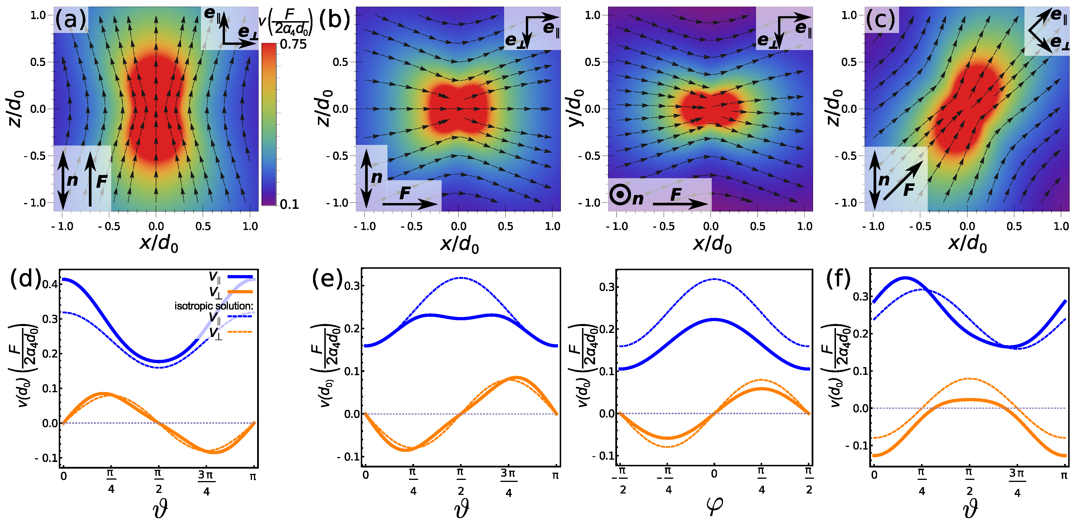
We use Green functions from Equations (24)–(32) to calculate the velocity profile in a weakly anisotropic homogeneous nematic due to a point force. In isotropic fluids, such Stokeslet profiles are associated with the dynamics of externally driven colloidal particles [3] or distinct microswimmers [32]. Differently as in the isotropic fluids, in the case of anisotropic nematic fluids, there are two principal solutions to the flow profile, corresponding to force being parallel or perpendicular to the director. For any other angle, the flow profile can be calculated as a linear combination of the two principal solutions due to the linearity of the Stokes equation. The nematic flow field generated by a point force can be written as:
where are Green functions given in Equations (24)–(28). The calculated flow profiles are shown in Figure 2. Figure 2a,e shows the flow profile of a point force that is aligned with the director. Similar as in the isotropic case (Figure 1), the flow profile retains the rotational symmetry around the force direction; however, the effective viscosity is lower along the director and more fluid is pumped in the direction of the force, meaning that less fluid is pumped from the perpendicular directions, thus reducing the curvature of the velocity field. If the force is aligned perpendicular to the director (Figure 2b,e), the flow profile shows only a mirror symmetry with respect to , , and planes. The spreading of the flow perpendicular to the force is more efficient along the director, showing larger magnitudes in the profile (Figure 2b,f opposed to profile in Figure 2b,e. At some angle between the force and the director ( in Figure 2c,f), the flow field retains only a symmetry with respect to the transformation. The flow magnitude is generally larger in the direction along the director. To generalise, our results demonstrate that for moderate anisotropy of the stress tensor that was chosen for graphical representation, flow profiles show obviously visible dependence on the direction of the applied force. We show three distinct cases, however, calculated results for the Green function allow for easy calculation of flow and pressure profiles at any angle between director and the driving force.
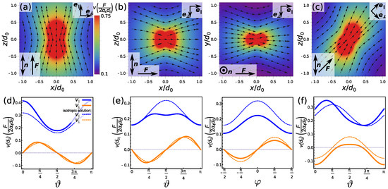
Figure 2.
Flow field of point force in nematic fluid oriented (a,d) parallel, (b,e) perpendicular, or (c,f) at angle to the director. The flow field decays as with the distance from the point force. In the bottom row, the velocity field component parallel to the force (along ) and perpendicular to the force (along ) at distance from the centre is shown as a function of azimuthal and polar angle. The value of can be chosen arbitrarily as long it is much larger than a swimmer size, since it only rescales the velocity magnitude. The values are compared to the isotropic case (dashed lines, see also Figure 1). Flow field is drawn for arbitrary values of the length and force F. Results show that for the given nematic anisotropy of the viscosity tensor, spreading of the momentum in the direction perpendicular to the director is suppressed, while the direction along the director offers much less resistance to the fluid flow. Note that graphs (d,e) are symmetrical with respect to case (or to case). In (f), which is no longer the case—the velocity field is tilted with respect to the direction of the applied force.
2.3. Flow Field of Force Dipole
Microswimmers with no external force applied have no Stokeslet contribution to the surrounding flow field. Instead, flow field is generated by higher moments of the distribution of forces exerted on the fluid, with force dipole being often the leading term. Indeed, typically the flow field of a force dipole exerted on the fluid falls as , where r is the distance from the swimmer. In addition, since higher moments of force distribution decay faster, dipolar flow field is the most pronounced in the far field of the velocity distribution, which was observed both in self-driven colloidal particles [5] and biological microswimmers [33].
More formally, the flow multipoles are introduced by using the linearity of the Stokes equation and writing the flow field of an arbitrary force distribution in the integral form as
Equation (34) is then Taylor expanded for distances much larger than the size of a microswimmers, which reveals separate contributions of force monopoles, dipoles, quadrupoles and other multipoles to the flow field of a swimmer, where the force dipole contribution equals [42]
and is the dipolar force moment. Typically, is decomposed into a traceless symmetrical tensor (stresslet) and an antisymmetrical tensor (rotlet):
The trace of was subtracted since the zero compressibility condition renders it ineffective to the fluid flow. The stresslet can be related to swimmer-imposed strain of the fluid and the rotlet to the net torque of the force distribution, with notably both mechanisms relevant in the complex swimming strokes of various micro-elements of micro-organisms.
2.3.1. Stresslet Flow Field in Nematics
To demonstrate stresslet flow field in a nematic, we plot the corresponding flow profiles of the far flow field due to two equal and opposite uniaxial point forces with size F acting on the fluid at a separation l (see scheme in Figure 1). Eigenvalues of the tensor are in that case , , and S, where . Negative S is associated with the pusher type of microswimmers, and positive values with puller type. In Figure 3, we plot flow fields of a puller microswimmer at different orientations of the axis of the applied forces with respect to the nematic director. Velocity field of a pusher has exactly the opposite direction of the flow. In order to calculate the appropriate flow field, one must first determine the components of the tensor. For example, Figure 3 shows a flow field due to two contractile forces along z-direction distance l apart. In that case, the components of the tensor equal: , and other components equal zero. The stresslet flow field is given by equation
where appropriate derivatives of the Green functions (Equations (24)–(28)) are easily calculated. Flow magnitude decays distinctly as ; therefore, all the main information about the flow field is contained in the angular dependence of the flow components, which we show in the bottom row of Figure 3 and compare them with the solution for the isotropic fluid, which has only a radial flow profile. If the force dipole is aligned along the director (Figure 3a,d), the flow field retains the radial-only flow profile and only the magnitude of the velocity field is changed:
here given in spherical coordinates , where the z-axis is defined by homogeneous director field. Radial-only flow profile in the aligned case is a necessary consequence of the symmetry imposed by the direction of the director and the force dipole, dependence of the flow, and flow incompressibility. However, in the case where the force dipole is perpendicular to the director (Figure 3b,c,f,g), flow field attains polar and azimuthal components. The profiles of the velocity magnitudes once again show rough correspondence with the regime of the lowest fluid resistance along the director. Upon tilting the force dipole at angle to the director (Figure 3d,h), the symmetry of the velocity profile is reduced and the difference to the radial profile is even more pronounced.
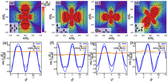
Figure 3.
Flow field of a force dipole at different orientations with respect to the director field. The bottom row shows radial and azimuthal (or polar) component of the velocity at distance from the centre as a function of azimuthal (or polar) angle compared to the result for isotropic fluids. (a,e) flow field of force dipole aligned with the director has only radial component. Note that radial flow field is characteristic for dipolar flow in isotropic fluids; however, in nematic fluids, there is still a difference between the magnitudes of the flow field between the isotropic case and a dipole aligned along the director due to anisotropic viscosity (see, e). In (a,e), the magnitude of the velocity field falls to zero at angle , whereas, in the isotropic case, the transition from inward to outward flow occurs at . At (b,c,f,g) or (d,h) , angles between force dipole and the director before radial flow configuration gains additional terms in the azimuthal and polar directions.
We have measured the volume around a dipolar swimmer, where the flow magnitude exceeds the value of (as some selected value). For a microswimmer aligned along the director, . If the force dipole is perpendicular to the director is reduced by . We expect similar behavior if one would consider the detection volume of a microswimmer [52]—a volume within which the gradients of the velocity field exceed a certain threshold. In nematic fluids, at the same force dipole, a microswimmer has lesser influence on the surrounding flow field if it is oriented at large angles with respect to the director.
2.3.2. Rotlet Flow
Motile parts of a microswimmer can in principle impose torques on the surrounding fluid, for example by rotating flagella [53]. However, for an isolated microswimmer, total torque applied on the fluid has to vanish [1]. To show the effect of torques in a nematic, we plot a flow field due to a point torque in Figure 4. A point torque in the y-direction was constructed by an antisymmetric force dipole tensor , where and other components equal zero. Flow field follows from Equation (35):
where derivatives of the Green functions (Equations (24)–(28)) need to be calculated. Compared to the isotropic fluid rotlet flows (Figure 1), Figure 4 shows concentric vortices around the origin deformed due to the anisotropy of the nematic fluid. The deformation occurs both in terms of magnitude of the velocity field, which is stretched along the director, and in terms of the shape of the velocity profile, which gains a radial component (compared to the isotropic case of only polar flow direction).
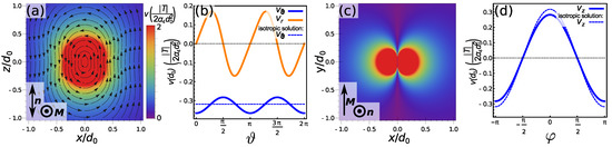
Figure 4.
Flow field of a point torque in nematic. (a,b) flow field due to torque that is perpendicular to the director. Compared to the isotropic case (b, see also Figure 1), the vortex stretches in the direction of the director; (c,d) same flow field in the cross-section. In (c), flow lines point in (out) of the plane.
2.4. Flow Fields of Sources and Sinks in Homogeneous Nematics
Flow sources and sinks represent another type of fundamental microfluidic elements that in various arrangements could also be associated with micro-organisms. More formally, point sources and sinks are another set of elementary solutions to the Stokes and compressibility equations [42]. They are characterized by zero force exerted on the fluid, but a non-zero velocity divergence at the position of the source or sink (in our case at ):
where A represents volumetric flow rate through a source (positive A) or a sink (negative A). Point-source dipoles or even more complex flow structures can be achieved using a linear combination of flow sources and sinks, as allowed by the linearity of the Stokes equation. We calculate the velocity and pressure profiles of a point source or sink in the homogeneous nematic and find the exact solutions in the reciprocal space and write the expressions in the real space in the limit of weak viscous anisotropy, using the same procedure as in Section 2.1. Notably, we obtain the velocity profile directly as analytic formulas. We write in terms of x-, y-, and z-components the compressibility condition (Equation (40)) and the Stokes equation for homogeneous director along the z-axis (Equations (4)–(6) for zero force) and perform the Fourier transform, similarly as was done in Equations (10)–(13). We obtain the solutions for velocity and pressure in the k-space:
We expand over and perform the inverse Fourier transform. The results for the velocity field in the spherical coordinates are:
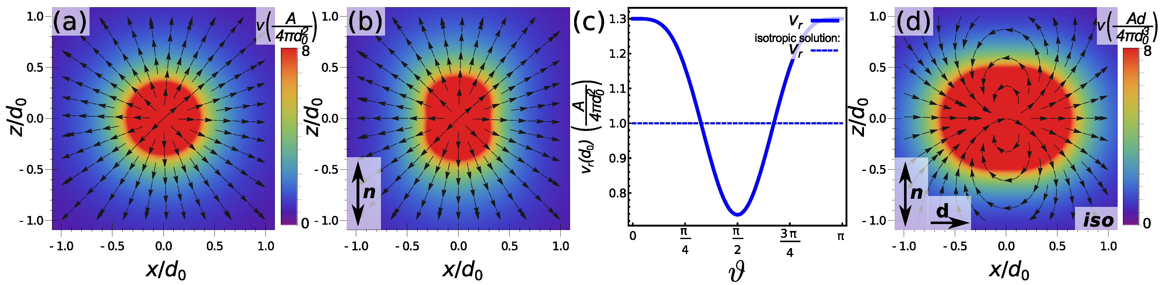
The velocity field of a point source is drawn in Figure 5. As shown in Equations (45) and (46), flow field has only a radial component. Similar to the stresslet flow in Figure 3a,d, the purely radial flow field is a consequence of the symmetry imposed by the director, flow incompressibility outside the source, and dependence of the flow. However, the anisotropy of the nematic medium results in the azimuthal dependence of the flow magnitude. The flow profile is dependent only on the and ratios of Leslie viscosities, whereas differently the pressure field is dependent on four viscosity coefficients (, , , ). In the isotropic fluids (), the pressure is a delta function at the point source. Other viscosity terms add terms that also depend on the azimuthal angle .
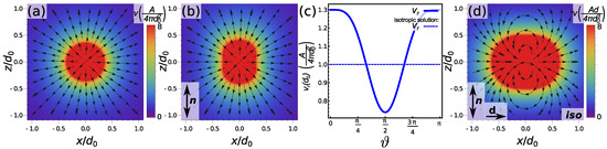
Figure 5.
Flow field of point source in (a) isotropic and (b) nematic fluid; and (c) radial flow velocity for a source flow (Equation (40)) shown for an isotropic and for a nematic fluid as a function of the azimuthal angle. In nematic fluid, the velocity field retains the radial direction; however, its amplitude as a function of azimuthal angle shows an increase along the z-axis—the director—and a decrease perpendicular to the director. Note that the flow field of a point sink is obtained directly by taking the opposite sign of the flow field of the source; (d) flow source and sink can be combined in a source dipole, here shown for isotropic medium.
2.5. Source Dipole Flow
Another elementary flow profile is a source dipole, which was shown to be an important contribution to the flow field of microswimmers [5]. It is formulated as a flow due to a point source and a point sink (each with strength A), which are separated by a dipole vector . The solution is obtained by using solutions for flow source and flow sink (as calculated In Section 2.4) and Taylor expanding the formulas for distances much larger than , giving
where , , and . Note that since the curl of the source flow is not zero—contrary to the isotropic case—we are not allowed to use the formalism of the potential flow [42] and have derived the above equation directly from Equation (45). For and , Equation (48) is equivalent to the solution for isotropic fluid [42] that is shown in Figure 5d. For non-zero values of and , source dipole flow is dependent on the orientation between the dipole and the director. Figure 6 shows flow profiles for (a,d) dipole parallel to the director, (b,c,f,g) dipole perpendicular to the director, and (d,h) dipole at angle to the director. Similar to other flow profiles discussed in this article, the magnitude of the velocity field is spread along the director field. In particular, at angle between the director and the dipole, flow magnitude profile is skewed compared to the isotropic case. The bottom row of Figure 6 gives a direct comparison to the isotropic solution in terms of radial and azimuthal (or polar) component of the velocity field.
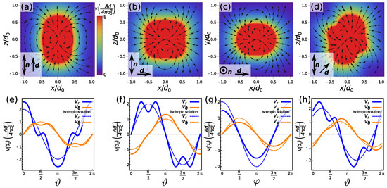
Figure 6.
Flow field of source dipole in nematic (Equation (48)) for the dipole aligned (a) parallel to the director; (b,c) perpendicular to the director, and (d) at angle to the director. The bottom row shows radial and azimuthal (or polar) components of the velocity field compared to the solution for isotropic fluid () for each of the cases above. Spreading of the velocity magnitude along the director is observed.
3. Discussion
3.1. Assumption of Weakly Anisotropic Nematic Fluid
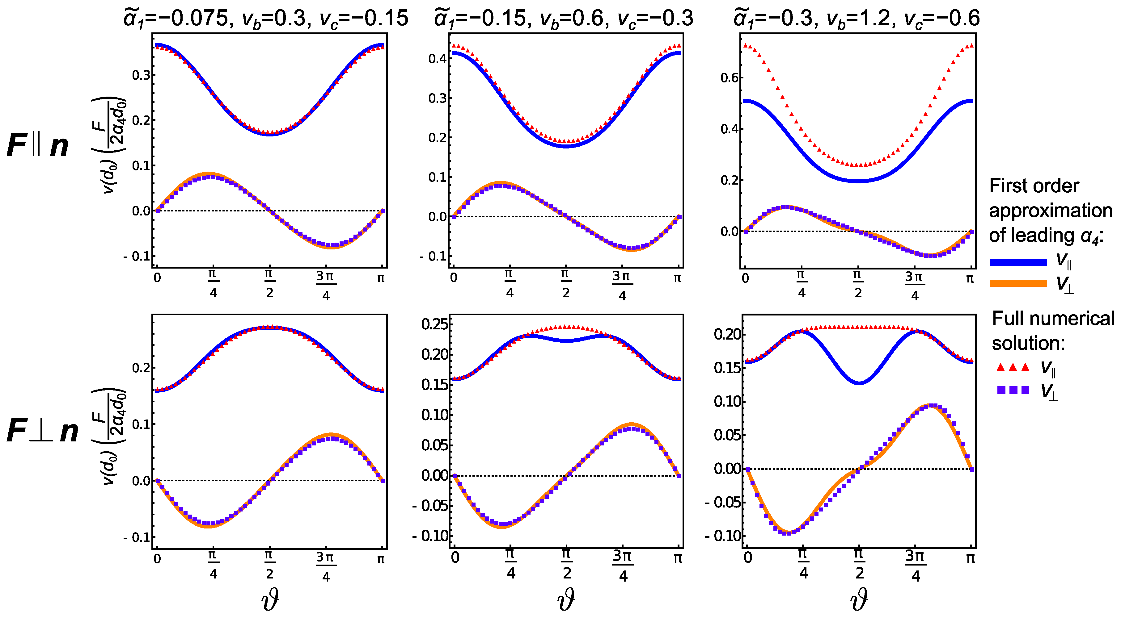
The demonstrated results for the Green function in nematics rely on the first order expansion in the ratio , where are six Leslie viscosities (coefficients), from which corresponds to isotropic stress. For the variety of nematic materials—i.e., the variety of regimes of values of the Leslie coefficients—this assumption is not necessarily justifiable in general. Therefore, we calculate in full—by numerical integration of the inverse Fourier transforms of the Green functions in Equations (10)–(13)—the corresponding flow profiles and compare them to the analytical flow profiles obtained through first order approximation of small . Note that in order to achieve good numerical convergence of the Fourier integrals, we have followed the approach in Ref. [31] and multiplied Equations (10)—(13) by a regularization function to eliminate large wavenumbers. We compare angular dependence of a Stokeslet flow for analytical and numerical results at the values of , , and used throughout this article and at higher/lower anisotropies. The comparison is shown in Figure 7. At smaller anisotropy (, , ), the full numerical calculations show an excellent match with first order approximations. At higher anisotropy (, , ), there is a clear mismatch between numerical and analytical results, indicating a clear overstep of the first-order approximation in . Analytical and numerical results for the viscosity coefficients used in the figures of this article (, , ) show some discrepancies, but they still capture similar behaviour. To generalise, the analytic to numeric comparison shows that, although slight discrepancies between the exact flow profiles are possible, flow profiles calculated in this article capture the essential response of flow fields to the anisotropy in the environment.
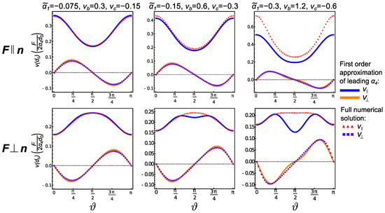
Figure 7.
Evaluation of small expansion assumption. Results for the point force along the director (first row) and perpendicular to the director (second row) obtained through the nematic Green function in Equations (24)–(29) are compared to the results obtained by numerical inverse Fourier transform of Equations (10)–(13) at distance from the point of force origin. The comparison is performed for the values of Leslie coefficients used throughout this article (middle column), values twice as small (first column) and twice as large (third column).
3.2. Deformations in the Director Profile
We have calculated the nematic Green functions by also assuming a homogeneous nematic director field (and also constant nematic degree of order). However, director deformations may occur due to anchoring of the nematic molecules on the surface of a microswimmer, anchoring at the confining interfaces, or due to backflow coupling to high velocity gradients. In a more complete analysis, simultaneously with the Stokes equation, an equation for the nematic order would have to be solved—for example the Ericksen–Leslie equation for the time derivative of the director alignment (Equation (3)). Due to complexity of the problem, the solution would most likely be only numerical. The resulting behavior could in principle include oscillatory solutions or even more complex temporal flows. However, experiments [19,20] and simulations [54] that consider interconnected behavior of nematic order and microswimmer-induced flow profiles typically observe stable trajectories of microswimmer motion and orientation. More complex temporal behavior though can occur at larger concentrations of microswimmers [20]. Notice that in real systems—such as swimmers—the centres of these flow multipoles are effectively within the body of the swimmer. Consequently, the exact singularity is always overlayed physically with the swimmer and only the flow fields already at some distance from the singularity affect the nematic. Additionally, surface anchoring at the body of the microfluidic object or possible external fields can further stabilize the nematodynamic behavior. Anchoring induced director field deformations due to a single swimmer and elastic interactions between individual swimmers, mediated by the deformation of the director field, can be assessed within the multipole expansion of the director field components [55]. In that case, the corrections to the homogeneous director field typically decay with a square of distance from the swimmer (in a case of a dipolar configuration) or faster. The torque on the nematic director due to material flow decays with the gradient of the velocity field, which in the leading (isotropic) approximation scales as and for a Stokeslet and stresslet, respectively. Director field deformations due to all of the above effects enter the divergence of the stress tensor and alter the velocity profile in the close proximity of a microswimmer. However, if at a sufficient distance from a microswimmer a homogeneous director far field is established, a general set of solutions for the flow field coincides with the results obtained in this article. A homogeneous director field could be additionally imposed by strong electric or magnetic fields. Finally, introducing and exploring the full role of nematic elasticity in the response of microswimmers is a highly exciting and interesting challenge.
3.3. Possible Application to Experiments
Recently, thorough investigative work has been conducted in the field of bacteria swimming in lyotropic nematics [19,20]. Due to anchoring of the nematic molecules on the surface of bacteria in lyotropic nematics, bacteria tend to align along the nematic director [18,19]. This is one of the rationale behind the control of the bacteria swimming direction by using patterned surface anchoring [56], similar to patterned anchoring in colloidal suspensions driven by liquid-crystal-enabled electrophoresis [57]. However, in principle, bacteria can change its direction and swim even perpendicular to the nematic director [58]. This means that, in principle, all orientations of force dipoles relative to the director field (as shown in Figure 3) are relevant to experimental applications. Ref. [18] shows how bacteria swimming along the nematic director can advect particles in the direction of its way, while particles which are positioned on the side of the swimming trajectory of the bacteria move only a little. This could be explained by the fact that the stresslet velocity field due to bacteria is strong mostly along the director, as shown in Figure 3 and is further affected by the strong anisotropy of the viscosity of the lyotropic nematic used in Ref. [18]. In Ref. [19], a collision of two bacteria swimming along the nematic director is discussed, leading to formation of chains. Notice though that if bacteria could be oriented at a notable angle relative to the director, such collision and/or binding events could further gain in complexity. As seen from Figure 3, non-radial terms in the flow field could in principle shift the colliding bacteria to non-colliding trajectories.
Emergent velocity profiles as discussed in this article are highly dependent on the microswimmer orientation with respect to the nematic director. This suggests that the swimming speed and the power consumption will also depend on the microswimmer orientation. Indeed, the existence of an effectively lower viscosity direction for swimming provides another or additional mechanism that affects the direction of swimming of the micro-swimmers [18,19]. Simulations for spherical squirmers show that pusher types tend to swim along the director, while pullers tend to swim perpendicular to the director [54]. It would be interesting to see how microswimmers would behave if the preferred alignment due to elasticity effects would be at large angles compared to the effective lower viscosity direction of swimming. Possibly, this could be achieved by different types of microswimmers, more complex shapes or anchoring conditions at the surface of a microswimmer, or possibly by using nematics with different material parameters.
The mutual interaction of bacteria depend on their concentration and the strength of force dipoles they impose upon the nematic. At high concentrations, interactions between bacteria are mediated through the deformation of the director field [18]. Instabilities due to the coupling of the orientation of bacteria, director field of the nematic, and bacterial flow can induce periodic stripe patterns in the director field [20]. However, at more dilute suspensions of bacteria, deformation of the director field might get suppressed by the homogeneous anchoring at the confining walls. In such cases, hydrodynamic interactions between bacteria could become of prime importance, including the effect of anisotropic viscosity as investigated in this article, suggesting that nematic flow profiles that mediate hydrodynamic interaction between microswimmers could significantly alter collective behavior of active particle suspensions.
4. Conclusions
Elementary solutions of the Stokes equation in nematic fluids are important from the perspective of understanding the nematic flows as well as in the context of swimming active particles in anisotropic fluids. We have derived Green functions for the Stokes equation for homogeneous nematic fluid (given by Equations (24)–(32)) under the approximations that (isotropic) viscosity is the leading viscosity coefficient in the Ericksen–Leslie stress tensor. Specifically, to obtain the solution, we have written Green functions for the Stokes equation for velocity and pressure in the Fourier space, expanded them to first order in anisotropic viscosity coefficients, and converted them back to real space. The calculated Green functions or their derivatives were then used to determine the flow field profiles of point forces (Equation (33)), stresslet (Equation (37)) and point torques (Equation (39)). Similarly, we have derived flow fields of point sources (sinks)(Equations (45)–(46)) and source dipoles (Equation (48)) in nematics. The solutions for the corresponding flow profiles are given as direct analytical formulas that could be used in further studies. The general qualitative consequence of anisotropic viscosity is that flow profiles change depending on the angle between the applied force (or stresslet or rotlet) and the nematic director. For viscosity coefficients used in the graphical representation of the derived equations, effective viscosity is smallest if flow direction coincides with the director. Therefore, for Stokeslet flow, the magnitude of the velocity field is the highest if the point force is aligned along the director (Figure 2a). If the alignment is at some angle, we observe a tilt of the velocity field towards the director (Figure 2c,f). The main characteristic of the stresslet flow in nematics is that, unless the force dipole is aligned along the director, flow field gains non-radial terms (Figure 3). Similarly, concentric vortices that form a rotlet flow in isotropic fluids get stretched along the nematic director in nematics (Figure 4). Source (sink) flow field remains only radial also in nematics; however, the flow magnitude shows an oval shape, oriented along the director (Figure 5). The obtained results were also critically assessed with regards to the two main assumptions of our approach—the leading isotropic viscosity and homogeneous nematic director—identifying the regimes of validity of the approach. In conclusion, our work provides an analytical insight into the field of elementary flow elements in nematic fluids—relevant for e.g., microswimmers in experiments in nematic liquid crystals or in biological fluids with anisotropic order—where the derived Green functions and flow profiles can be used to further construct flow fields of other—in principle arbitrary—swimmers and model their dynamics.
Acknowledgments
The authors thank Jörn Dunkel for stimulating discussions on topics related to this work. Funding from the Slovenian Research Agency (ARRS) through grants P1-0099, J1-7300, L1-8135, the ARRS Younger researcher program (researcher number 37526), and the US Air Force Office of Scientific Research, European Office of Aerospace Research and Development research project Nematic Colloidal Tilings as Tunable Soft Metamaterials (Grant No. FA9550-15-1-0418) is acknowledged.
Author Contributions
Ž.K. performed the calculations. M.R. supervised the work. Both authors wrote the paper.
Conflicts of Interest
The authors declare no conflict of interest.
References
- Lauga, E.; Powers, T.R. The hydrodynamics of swimming microorganisms. Rep. Prog. Phys. 2009, 72, 096601. [Google Scholar] [CrossRef]
- Elgeti, J.; Winkler, R.G.; Gompper, G. Physics of microswimmers—Single particle motion and collective behavior: A review. Rep. Prog. Phys. 2015, 78, 056601. [Google Scholar] [CrossRef] [PubMed]
- Bechinger, C.; Leonardo, R.D.; Löwen, H.; Reichhardt, C.; Volpe, G.; Volpe, G. Active particles in complex and crowded environments. Rev. Mod. Phys. 2016, 88, 045006. [Google Scholar] [CrossRef]
- Purcell, E.M. Life at low Reynolds number. Am. J. Phys. 1977, 45, 3–11. [Google Scholar] [CrossRef]
- Zöttl, A.; Stark, H. Emergent behavior in active colloids. J. Phys. Condens. Matter 2016, 28, 253001. [Google Scholar] [CrossRef]
- Sokolov, A.; Apodaca, M.M.; Grzybowski, B.A.; Aranson, I.S. Swimming bacteria power microscopic gears. Proc. Natl. Acad. Sci. USA 2010, 107, 969–974. [Google Scholar] [CrossRef] [PubMed]
- Thampi, S.P.; Doostmohammadi, A.; Shendruk, T.N.; Golestanian, R.; Yeomans, J.M. Active micromachines: Microfluidics powered by mesoscale turbulence. Sci. Adv. 2016, 2, e1501854. [Google Scholar] [CrossRef] [PubMed]
- Kim, M.J.; Breuer, K.S. Enhanced diffusion due to motile bacteria. Phys. Fluids 2004, 16, L78–L81. [Google Scholar] [CrossRef]
- Pushkin, D.O.; Shum, H.; Yeomans, J.M. Fluid transport by individual microswimmers. J. Fluid Mech. 2013, 726, 5–25. [Google Scholar] [CrossRef]
- Hatwalne, Y.; Ramaswamy, S.; Rao, M.; Simha, R. Rheology of active-particle suspensions. Phys. Rev. Lett. 2004, 92, 118101. [Google Scholar] [CrossRef] [PubMed]
- López, H.M.; Gachelin, J.; Douarche, C.; Auradou, H.; Clément, E. Turning bacteria suspensions into superfluids. Phys. Rev. Lett. 2015, 115, 028301. [Google Scholar] [CrossRef] [PubMed]
- Fung, Y.C. Biomechanics: Mechanical Properties of Living Tissues; Springer: Heidelberg, Germany, 1981. [Google Scholar]
- Luby-Phelps, K. Cytoarchitecture and physical properties of pytoplasm: volume, viscosity, diffusion, intracellular surface area. Int. Rev. Cytol. 1999, 192, 189–221. [Google Scholar]
- Rey, A.D. Liquid crystal models of biological materials and processes. Soft Matter 2010, 6, 3402–3429. [Google Scholar] [CrossRef]
- Kumar, A.; Galstian, T.; Pattanayek, S.K.; Rainville, S. The Motility of bacteria in an anisotropic liquid environment. Mol. Cryst. Liq. Cryst. 2013, 574, 33–39. [Google Scholar] [CrossRef]
- Toner, J.; Löwen, H.; Wensink, H.H. Following fluctuating signs: Anomalous active superdiffusion of swimmers in anisotropic media. Phys. Rev. E 2016, 93, 062610. [Google Scholar] [CrossRef] [PubMed]
- Mushenheim, P.C.; Trivedi, R.R.; Roy, S.S.; Arnold, M.S.; Weibel, D.B.; Abbott, N.L. Effects of confinement, surface-induced orientations and strain on dynamical behaviors of bacteria in thin liquid crystalline films. Soft Matter 2015, 11, 6821–6831. [Google Scholar] [CrossRef] [PubMed]
- Sokolov, A.; Zhou, S.; Lavrentovich, O.D.; Aranson, I.S. Individual behavior and pairwise interactions between microswimmers in anisotropic liquid. Phys. Rev. E 2015, 91, 013009. [Google Scholar] [CrossRef] [PubMed]
- Mushenheim, P.C.; Trivedi, R.R.; Tuson, H.H.; Weibel, D.B.; Abbott, N.L. Dynamic self-assembly of motile bacteria in liquid crystals. Soft Matter 2013, 10, 88–95. [Google Scholar] [CrossRef] [PubMed]
- Zhou, S.; Sokolov, A.; Lavrentovich, O.D.; Aranson, I.S. Living liquid crystals. Proc. Natl. Acad. Sci. USA 2014, 111, 1265–1270. [Google Scholar] [CrossRef] [PubMed]
- Trivedi, R.R.; Maeda, R.; Abbott, N.L.; Spagnolie, S.E.; Weibel, D.B. Bacterial transport of colloids in liquid crystalline environments. Soft Matter 2015, 11, 8404–8408. [Google Scholar] [CrossRef] [PubMed]
- Lavrentovich, O.D. Active colloids in liquid crystals. Curr. Opin. Colloid Interface Sci. 2016, 21, 97–109. [Google Scholar] [CrossRef]
- Krieger, M.S.; Spagnolie, S.E.; Powers, T.R. Locomotion and transport in a hexatic liquid crystal. Phys. Rev. E 2014, 90, 052503. [Google Scholar] [CrossRef] [PubMed]
- Krieger, M.S.; Spagnolie, S.E.; Powers, T. Microscale locomotion in a nematic liquid crystal. Soft Matter 2015, 11, 9115–9125. [Google Scholar] [CrossRef] [PubMed]
- Heuer, H.; Kneppe, H.; Schneider, F. Flow of a nematic liquid crystal around a sphere. Mol. Cryst. Liq. Cryst. 1992, 214, 43–61. [Google Scholar] [CrossRef]
- Kneppe, H.; Schneider, F.; Schwesinger, B. Axisymmetrical flow of a nematic liquid crystal around a sphere. Mol. Cryst. Liq. Cryst. 1991, 205, 9–28. [Google Scholar] [CrossRef]
- Kozachok, M.V.; Lev, B.I. Analytical calculation of the Stokes drag of the spherical particle in a nematic liquid crystal. Condens. Matter Phys. 2014, 17, 79–86. [Google Scholar] [CrossRef]
- Stark, H.; Ventzki, D.; Reichert, M. Recent developments in the field of colloidal dispersions in nematic liquid crystals: the Stokes drag. J. Phys. Condens. Matter 2003, 15, S191. [Google Scholar] [CrossRef]
- Stark, H.; Ventzki, D. Stokes drag of spherical particles in a nematic environment at low Ericksen numbers. Phys. Rev. E 2001, 64, 031711. [Google Scholar] [CrossRef] [PubMed]
- Pokrovskii, V.; Tskhai, A. Slow motion of a particle in a weakly anisotropic viscous fluid. J. Appl. Math. Mech. 1986, 50, 391–394. [Google Scholar] [CrossRef]
- Gómez-González, M.; del Álamo, J.C. Flow of a viscous nematic fluid around a sphere. J. Fluid Mech. 2013, 725, 299–331. [Google Scholar] [CrossRef]
- Drescher, K.; Goldstein, R.E.; Michel, N.; Polin, M.; Tuval, I. Direct measurement of the flow field around swimming microorganisms. Phys. Rev. Lett. 2010, 105, 168101. [Google Scholar] [CrossRef] [PubMed]
- Drescher, K.; Dunkel, J.; Cisneros, L.H.; Ganguly, S.; Goldstein, R.E. Fluid dynamics and noise in bacterial cell-cell and cell-surface scattering. Proc. Natl. Acad. Sci. USA 2011, 108, 10940–10945. [Google Scholar] [CrossRef] [PubMed]
- Pushkin, D.O.; Yeomans, J.M. Fluid mixing by curved trajectories of microswimmers. Phys. Rev. Lett. 2013, 111, 188101. [Google Scholar] [CrossRef] [PubMed]
- Alexander, G.P.; Yeomans, J.M. Dumb-bell swimmers. EPL 2008, 83, 34006. [Google Scholar] [CrossRef]
- Alexander, G.P.; Pooley, C.M.; Yeomans, J.M. Hydrodynamics of linked sphere model swimmers. J. Phys. Condens. Matter 2009, 21, 204108. [Google Scholar] [CrossRef] [PubMed]
- Baskaran, A.; Marchetti, M.C. Statistical mechanics and hydrodynamics of bacterial suspensions. Proc. Natl. Acad. Sci. USA 2009, 106, 15567–15572. [Google Scholar] [CrossRef] [PubMed]
- Saintillan, D.; Shelley, M. Instabilities and pattern formation in active particle suspensions: Kinetic theory and continuum simulations. Phys. Rev. Lett. 2008, 100, 178103. [Google Scholar] [CrossRef] [PubMed]
- Mathijssen, A.J.T.M.; Doostmohammadi, A.; Yeomans, J.M.; Shendruk, T.N. Hydrodynamics of micro-swimmers in films. J. Fluid Mech. 2016, 806, 35–70. [Google Scholar] [CrossRef]
- Reigh, S.Y.; Zhu, L.; Gallaire, F.; Lauga, E. Swimming with a cage: Low-Reynolds-number locomotion inside a droplet. Soft Matter 2017, 13, 3161–3173. [Google Scholar] [CrossRef] [PubMed]
- Marchetti, M.C.; Joanny, J.F.; Ramaswamy, S.; Liverpool, T.B.; Prost, J.; Rao, M.; Simha, R.A. Hydrodynamics of soft active matter. Rev. Mod. Phys. 2013, 85, 1143–1189. [Google Scholar] [CrossRef]
- Pozrikidis, C. Introduction to Theoretical and Computational Fluid Dynamics, 2nd ed.; Oxford University Press: New York, NY, USA, 2011. [Google Scholar]
- De Gennes, P.G.; Prost, J. Physics of Liquid Crystals; Oxford University Press: New York, NY, USA, 1993. [Google Scholar]
- Denniston, C.; Orlandini, E.; Yeomans, J. Lattice Boltzmann simulations of liquid crystal hydrodynamics. Phys. Rev. E 2001, 63, 056702. [Google Scholar] [CrossRef] [PubMed]
- Giomi, L.; Kos, Ž.; Ravnik, M.; Sengupta, A. Cross-talk between topological defects in different fields revealed by nematic microfluidics. Proc. Natl. Acad. Sci. USA 2017, 114, E5771–E5777. [Google Scholar] [CrossRef] [PubMed]
- Taratuta, V.G.; Hurd, A.J.; Meyer, R.B. Light-scattering study of a polymer nematic liquid crystal. Phys. Rev. Lett. 1985, 55, 246–249. [Google Scholar] [CrossRef] [PubMed]
- Jamieson, A.M.; Gu, D.; Chen, F.; Smith, S. Viscoelastic behavior of nematic monodomains containing liquid crystal polymers. Prog. Polym. Sci. 1996, 21, 981–1033. [Google Scholar] [CrossRef]
- Kuzuu, N.; Doi, M. Constitutive equation for nematic liquid crystals under weak velocity gradient derived from a molecular kinetic equation. J. Phys. Soc. Jpn. 1983, 52, 3486–3494. [Google Scholar] [CrossRef]
- Herba, H.; Szymański, A.; Drzymala, A. Experimental test of hydrodynamic theories for nematic liquid crystals. Mol. Cryst. Liq. Cryst. 1985, 127, 153–158. [Google Scholar] [CrossRef]
- Cui, M.; Kelly, J.R. Temperature dependence of visco-elastic properties of 5CB. Mol. Cryst. Liq. Cryst. 1999, 331, 49–57. [Google Scholar] [CrossRef]
- Adkins, G. Three-dimensional Fourier transforms, integrals of spherical Bessel functions, and novel delta function identities. arXiv, 2013; arXiv:1302.1830. [Google Scholar]
- Doostmohammadi, A.; Stocker, R.; Ardekani, A.M. Low-Reynolds-number swimming at pycnoclines. Proc. Natl. Acad. Sci. USA 2012, 109, 3856–3861. [Google Scholar] [CrossRef] [PubMed]
- Hu, J.; Yang, M.; Gompper, G.; Winkler, R.G. Modelling the mechanics and hydrodynamics of swimming E. coli. Soft Matter 2015, 11, 7867–7876. [Google Scholar] [CrossRef] [PubMed]
- Lintuvuori, J.; Würger, A.; Stratford, K. Hydrodynamics defines the stable swimming direction of spherical squirmers in a nematic liquid crystal. Phys. Rev. Lett. 2017, 119, 068001. [Google Scholar] [CrossRef] [PubMed]
- Lubensky, T.C.; Pettey, D.; Currier, N. Topological defects and interactions in nematic emulsions. Phys. Rev. E 1998, 57, 610–625. [Google Scholar] [CrossRef]
- Peng, C.; Turiv, T.; Guo, Y.; Wei, Q.H.; Lavrentovich, O.D. Command of active matter by topological defects and patterns. Science 2016, 354, 882–885. [Google Scholar] [CrossRef] [PubMed]
- Hernàndez-Navarro, S.; Tierno, P.; Farrera, J.A.; Ignés-Mullol, J.; Sagués, F. Reconfigurable swarms of nematic colloids controlled by photoactivated surface patterns. Angew. Chem. Int. Ed. 2014, 53, 10696–10700. [Google Scholar] [CrossRef] [PubMed]
- Zhou, S.; Tovkach, O.; Golovaty, D.; Sokolov, A.; Aranson, I.S.; Lavrentovich, O.D. Dynamic states of swimming bacteria in a nematic liquid crystal cell with homeotropic alignment. New J. Phys. 2017, 19, 055006. [Google Scholar] [CrossRef]


© 2018 by the authors. Licensee MDPI, Basel, Switzerland. This article is an open access article distributed under the terms and conditions of the Creative Commons Attribution (CC BY) license (http://creativecommons.org/licenses/by/4.0/).