Article

A Non-Hydrostatic Depth-Averaged Model for Hydraulically Steep Free-Surface Flows

by
Yebegaeshet T. Zerihun
David & James–Engineering and Environmental Consultancy, 204 Albion Road, Victoria 3350, Australia
Fluids 2017, 2(4), 49; https://doi.org/10.3390/fluids2040049
Submission received: 5 August 2017 / Revised: 16 September 2017 / Accepted: 18 September 2017 / Published: 23 September 2017
(This article belongs to the Special Issue Advances in Hydrodynamics)

Abstract

:
This study describes the results of a numerical investigation aimed at developing and validating a non-hydrostatic depth-averaged model for flow problems where the horizontal length scales close to flow depth. For such types of problems, the steep-slope shallow-water equations are inadequate to describe the two-dimensional structure of the curvilinear flow field. In the derivation of these equations, the restrictive assumptions of negligible bed-normal acceleration and bed curvature were employed, thus limiting their applicability to shallow flow situations. Herein, a Boussinesq-type model is deduced from the depth-averaged energy equation by relaxing the weakly-curved flow approximation to deal with the non-hydrostatic steep flow problems. The proposed model is solved with an implicit finite difference scheme and then applied to simulate steady free-surface flow problems with strong curvilinear effects. The numerical results are compared to experimental data, resulting in a reasonable overall agreement. Further, it is shown that the discharge characteristics of free flow over a round-crested weir are accurately described by using a Boussinesq-type approximation, and the drawbacks arising from a standard hydrostatic approach are overcome. The suggested numerical method to determine the discharge coefficient can be extended and adopted for other types of short-crested weirs.

1. Introduction

The dynamics of open channel flows have been the subject of many experimental and numerical studies in the past. The outcomes of such studies have been used for developing effective resource management strategies for natural and regulated river flows, as well as for assessing the transports of pollutant and nutrients including eco-geomorphic interactions in rivers. They have also been applied to develop numerical tools for evaluating different design alternatives for a complex hydraulic structure where the streamline vertical curvatures induced by a curved boundary significantly affect the free overflow characteristics. Maximising the hydraulic performance of such an overflow structure is still an issue of continually growing interest for practicing engineers and decision makers. A practical approach based on a higher-order approximation for the effects of the vertical acceleration of the curvilinear flow is necessary to address this issue.
In practice, computational models based on the steep-slope form of the shallow-water equations have been commonly used to analyse free-surface flow problems. Such models are computationally efficient and are able to simulate many shallow flow features quite satisfactorily. The governing equations of the models were developed by using the restrictive assumptions of negligible bed-normal acceleration and bed curvature (see, e.g., [1,2,3]). Consequently, these lower-order equations are not able to describe adequately the necessary flow details over the vertical dimension and hence, do not provide accurate solutions for flow problems where the effects of the dynamic pressure are significant [4,5,6].
Many investigators proposed more complete formulations of the hydrodynamic equations of an open channel flow by accounting for a non-hydrostatic pressure distribution effect, rather than resorting to the shallow-water theory or the results of more expensive physical model tests. Fawer [7] was one of the earliest investigators to extend the energy equation by taking into account the effects of the free-surface and the bed curvatures. His method was based on the assumptions of irrotational flow and a nonlinear variation of streamline vertical curvature from the bed to the free surface. Fawer’s approach resulted in second-order open-channel flow equations for a steady curved flow, which are rewritten here as
E = q 2 2 g H 2 + q 2 g H ( N + 2 ) H x x + q 2 2 g H Z x x + H
p b γ = H + q 2 N g H ( N + 1 ) Z x x + q 2 g H ( N + 1 ) η x x
d E d x = S 0 S e
where H is the local flow depth measured vertically; q is the unit discharge; g is acceleration due to gravity; E is the specific energy head; S 0 is the local bed slope; S e is the energy gradient; Z x x and η x x are the second derivatives of the bed and the free-surface profiles, respectively; p b is the bottom pressure; γ is the unit weight of the fluid; and N is an exponent for the assumed variation of the streamline curvature. In this method, however, the effects of streamline inclination have not been considered. The familiar specific energy equation for parallel-streamline flow in a horizontal bed channel can be deduced from Equation (1a) by neglecting all the derivative terms. Using similar closure hypotheses, Hager and Hutter [8] developed a Boussinesq-type energy equation in a streamline coordinate system. However, the application of their equation is limited to a geometrically mild-slope flow situation. Hager [9] extended the method of the derivation by considering a relatively higher-order of approximation for the streamline curvature effects as compared to Hager and Hutter’s [8] method. As a result of this, his equation is applicable to flow problems with moderately sloped (up to 30°) and curved streamlines. Using an analogous but a higher-order method based on the Picard iteration, Matthew [10] developed a Boussinesq-type potential-flow equation in a Cartesian coordinate system. Matthew’s [10] approach was later applied by Castro-Orgaz and Hager [11] for analysing unsteady free-surface flow problems, which was originally proposed by Matthew for such problems. Similar to Fawer’s approach, the Matthew approach for the extended energy equation theoretically valids for free-surface flows with weakly sloped and curved streamlines. For curvilinear flows in a moderate slope channel, Zerihun [12] investigated Matthew’s equation and found satisfactory agreement with their experiments. Following the method proposed by Benjamin and Lighthill [13], Marchi [14,15] presented a higher-order one-dimensional equation, which is identical in structure to Matthew’s equation, using a Cartesian coordinate system. Other investigators [16] extended the Bernoulli equation for moderately curved free-surface flows closely following Hager’s [9] approach. All these Boussinesq-type equations [8,9,16] were derived by taking the flow depth as the vertical projection of an equipotential curve rather than a true vertical distance between the channel bed and the free surface, as was done by Matthew [10]. This implies that the application of such equations to curvilinear flow problems requires further simplifying assumptions on the structure of the flow for estimating the undetermined parameters. For a steep open-channel flow over curved surfaces, Berger [2] extended the Dressler [17] perturbation approach to derive the curved-flow equations. Analogous to Dressler’s equations, however, his equations do not separate the effects of the curvature of the free surface from the bed curvature and reduce to the Saint-Venant equations for curvilinear flows in a mild-slope channel. This significant loss of information on the vertical structure of the flow field is the drawback of this approach as compared to earlier Boussinesq-type methods. For ideal fluid flows, a depth-averaged form of Bernoulli’s equation, along with correction coefficients for the actual distributions of velocity and pressure in the flow field, has been proposed by Jaeger [18], Liggett [19] and Chanson [20]. Recently, Castro-Orgaz and Chanson [21] further investigated this depth-averaged equation for curvilinear potential-flow problems. However, the application of this equation to such types of flow problems requires a prior knowledge of the distributions of the pressure and the kinetic-energy correction coefficients.
As described above, most of the previous studies on the development of the hydrodynamic equations of a curvilinear free-surface flow, with the exception of Berger’s [2] and Hager’s [9] methods, are based on the assumption of slightly curved and sloped streamlines. Such an approximation may restrict the range of application of the equations (see, e.g., [12]). The method of deriving the governing equations of a curved-streamline flow based on the energy principle, therefore, must address the effects of nonuniform velocity and non-hydrostatic pressure distributions, as well as a hydraulically steep slope effect. This research work is motivated by the desire to overcome the limitations associated with the numerical modelling of free-surface flows with curvilinear streamlines, which involves further generalisation of the depth-averaged energy method by relaxing the weakly-curved flow approximation. The proposed approach results in a hydrodynamic model that incorporates a higher-order correction for the effects of both the vertical curvatures of the streamline and the steep free-surface slope, thereby accurately describing the structure of the rapidly-varied flow situations. Therefore, the main objectives of this study are: (i) to develop a higher-order depth-averaged model that includes more information on the vertical details of the flow structure; (ii) to provide a comprehensive assessment of the feasibility of the model for practical steady flow problems with a strong curvilinear effect; (iii) to assess the influence of the weakly-curved flow simplifying approximation on the solutions of the problems; and (iv) to demonstrate the validity of the model results by a number of existing experimental data. The performance of the proposed model is tested by considering a non-hydrostatic flow problem with continuous free-surface profiles such as transcritical flows over sharply-curved hydraulic structures. The two-dimensional (2D) characteristics of the selected problems enable us to examine how the model behaves at a flow transition from subcritical to supercritical state. Also, the numerical results of these problems provide vital information regarding the significance of the higher-order terms of the model equations, which can be used to simplify the equations for a specific type of practical application. It is worth noting that the method presented in this study is limited to the analysis of non-viscous flows.
Following a brief summary of the derivation of the governing equations, the paper presents a description of the main features of the computational model namely the spatial discretisation of the equations. The solution procedures for the resulting nonlinear discretised equations with reference to the case studies are outlined. The boundary conditions of the numerical model are also discussed. A brief discussion of the model results is presented by comparing them to experimental data from the literature. The paper is ended by conclusive remarks.

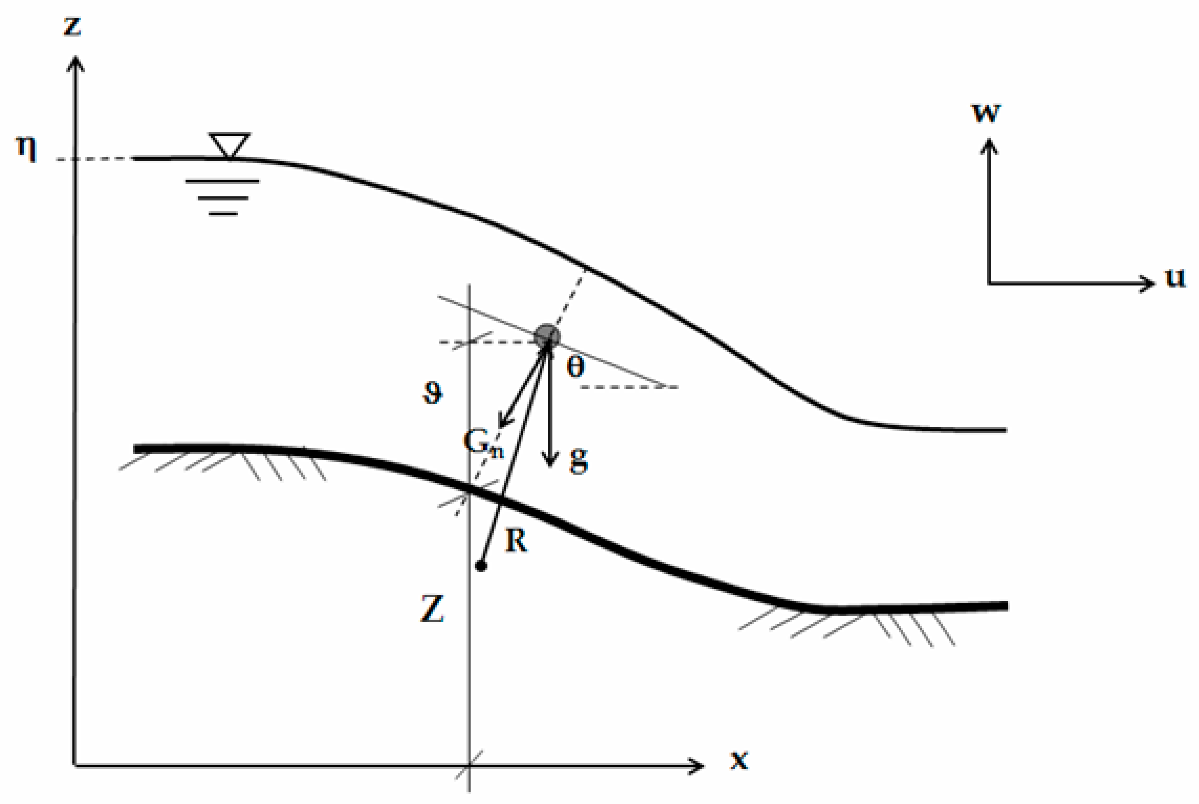
2. Governing Equations
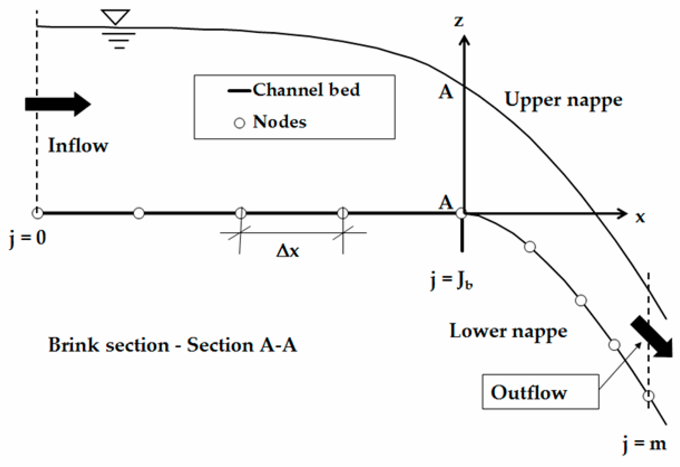
Consider the longitudinal profile of a rapidly-varied flow in an open channel, as shown in Figure 1. Let there be a Cartesian coordinate system, where x is horizontal along the channel, y is horizontal in the transverse direction; and z is vertically upward. For steady 2D flow, the depth-averaged energy equation may be written as (see, e.g., [18,19])
H e = 1 q Z η ( u 2 + w 2 2 g + p ρ g + ϑ ) u d z
where H e denotes the total energy head; u is the velocity in the streamwise x -direction; w is the vertical velocity; ϑ = ( z Z ) cos 2 θ s + Z ; z is the elevation of a point in the flow field; Z is the bed elevation; η refers to the free-surface elevation; ρ is the density of the fluid; p is the pressure; and θ s is the angle of the free-surface streamline (denoted by the subscript s ) with the horizontal. As noted by Jaeger [18] and Rouse [22], Equation (2) describes the depth-averaged total energy, determined between the free-surface and bed streamlines for an incompressible and non-viscous fluid.
The distribution of the horizontal velocity at a vertical section may be approximated by its depth-averaged value as [23]
u = q H
By applying Leibnitz’s rule, the integration of the 2D continuity equation from z to η can be written in the form:
z η u x d z + z η w z d z = x z η u ( z ) d z + u ( z ) z x u ( η ) η x + w s w = 0
Inserting Equation (3) into Equation (4) and applying the free-surface kinematic boundary condition, w s = η x u s , results for the vertical velocity distribution in
w = q H H x ζ + q H Z x
ζ = z Z η Z
where u s and w s are the horizontal and vertical velocity components at the free surface, respectively; and ζ is a non-dimensional vertical coordinate. In the above equations, the subscript x denotes differentiation with respect to the horizontal axis.
If a n ( = κ u 2 sec 2 θ ) is the normal acceleration, the Euler equation of motion along a reference axis normal to the local free-surface can be expressed as follows (see, e.g., [24,25]):
1 ρ p n = G n ξ κ u 2 sec 2 θ
where κ ( = 1 / R ) is the local streamline curvature; p / n is the pressure gradient; ξ accounts for the deviation of the free-surface slope from the local streamline inclination; R is the radius of curvature; and G n = g cos θ s . The contribution of the streamline geometry parameter, β ( = ξ κ sec 2 θ ) , in Equation (6) may be approximated by assuming a linear distribution across the flow depth as
β = ( η x x 1 + ( η x ) 2 Z x x 1 + ( η x ) 2 ( 1 + ( Z x ) 2 ) ) ζ + Z x x 1 + ( η x ) 2 ( 1 + ( Z x ) 2 )
ξ = 1 1 + ( z x ) 2 1 + ( η x ) 2 + z x η x 1 + ( z x ) 2 1 + ( η x ) 2
To obtain the vertical component of the pressure gradient, n is substituted by z cos θ s in Equation (6). Inserting Equations (3) and (7a) into Equation (6) and then integrating the resulting expression in the z -direction using the dynamic boundary condition, p ( η ) = 0 , yields the pressure distribution equation for flow in a rectangular channel
p γ = ( 1 ζ ) H ω 1 + q 2 Z x x ( 1 ζ ) g H ω 1 ω 2 + q 2 2 g H ω 1 ( η x x Z x x ω 2 ) ( 1 ζ 2 )
where Z x ( = S 0 ) is the local bed gradient of the channel; ω 1 = 1 + ( η x ) 2 ; and ω 2 = 1 + ( Z x ) 2 .
The first term on the right-hand side of Equation (8) represents the modified hydrostatic pressure as a result of the effect of the steep streamwise gradient, while the second and third terms stand for the component of the dynamic pressure due to the effects of the vertical acceleration. For the case of gradually-varied free-surface flow with negligible curvature of streamline in a mild-slope channel, the contributions of the free-surface and bed curvatures terms are insignificant ( η x x = Z x x = 0 and ω 1 = ω 2 1.0 ). Under this flow condition, Equation (8) reduces to the hydrostatic pressure equation which corresponds to the shallow-water theory. The pressure at the bed of the channel can be deduced from Equation (8) by setting ζ = 0 as
p b γ = H ω 1 + q 2 2 g H ω 1 ( η x x + Z x x ω 2 )
Substituting Equations (3), (5a) and (8) into Equation (2) and then integrating the resulting expression with respect to z over the flow depth gives the following equation for steady flow in a rectangular channel:
H e = q 2 2 g H 2 ( α + Z x 2 + H x Z x + ( H x ) 2 3 ) + q 2 3 g H ω 1 H x x + q 2 Z x x 6 g H ω 1 ( 2 ω 2 + 1 ω 2 ) + H ω 1 + Z
d H e d x = S f
where α is the Coriolis velocity correction coefficient; and S f is the friction slope. Equation (10a) is a generalised higher-order equation for steady 2D hydraulically steep flow problems where the vertical accelerations play a significant role. Although this equation was developed based on the assumption of non-viscous flows, it incorporates a term that takes into account the effects of boundary friction (but not internal) in the streamwise energy balance, as in Serre [23]. For the case of quasi-uniform free-surface flows in a constant slope channel ( α 1.0 ), Equation (10a) reduces to the steep-slope form of the energy equation [26],
H e = q 2 2 g H 2 ( 1 + Z x 2 ) + H ( 1 + η x 2 ) + Z
whereas Fawer’s [7] equation degenerates to the Bernoulli equation, which corresponds to the zeroth-order approximation of Equation (10a). It is evident that Equation (1a) can be deduced from Equation (10a) by neglecting all products of derivatives. All these reveal that the main differences between the present model and earlier results by Fawer [7] and Matthew [10] are all in the nonlinear coefficients of the spatial derivative terms, as described by Equation (13). In Equation (10a), these coefficients and the derivative terms take into account the effect of steep free-surface slope besides the effect of the vertical acceleration of the flow, and their associated effects on the velocity and pressure distributions. Differentiating Equation (11) with respect to x results in the following equation (assuming that η x Z x ) for a gradually-varied flow in a steep-slope channel [4]:
d H d x = S 0 S f 1 ( 1 + Z x 2 ) q 2 g H 3 ( 1 + Z x 2 )
The conventional hydraulic approximation can be obtained by neglecting the steep-slope effect in Equation (12), 1 + Z x 2 1 , to give the classical version of this equation for such a type of free-surface flow in a mild-slope channel.
In this study, Equations (9) and (10a) will be employed to obtain detailed descriptions of the local and global flow characteristics of a curved-streamline flow in a rectangular channel. In these equations, the unknowns to be solved numerically using an implicit finite difference scheme, which will be described in the following section, are the flow depth and the bottom pressure. The numerical solutions of the equations will be compared to measurements in order to determine the validity of the proposed model for non-hydrostatic free-surface flow problems.

3. Numerical Method

Equation (10a) is a second-order ordinary differential equation which requires two boundary conditions to be prescribed either at the upstream and downstream ends or at the upstream end only. These two extreme sections may be located in a weakly non-hydrostatic flow region, so that lower-order equations can be applied to compute the boundary values. Further discussion on the implementation of boundary conditions with reference to the case studies will be presented in the next section. For the purpose of discretisation, Equation (10a) can be rewritten in a more compact form as
λ 0 , j H x x , j + λ 1 , j ( H x , j ) 2 + λ 2 , j H x , j + λ 3 , j = 0
where λ 0 , j , λ 1 , j , λ 2 , j and λ 3 , j are the nonlinear coefficients of the governing equation at node j and are expressed by:
λ 0 , j = q 2 3 g H j ω 1 , j
λ 1 , j = q 2 6 g H j 2
λ 2 , j = q 2 2 g H j 2 Z x , j
λ 3 , j = q 2 ( α + Z x , j 2 ) 2 g H j 2 + q 2 Z x x , j 6 g H j ω 1 , j ( 2 ω 2 , j + 1 ω 2 , j ) + H j ω 1 , j + Z j ( H e , 0 H l , j )
where H e , 0 is the total energy head at the inflow section; and H l , j is the head loss between the inflow section and a downstream section at node j . The first and second spatial derivative terms in Equation (13) are discretised using the four-point finite difference approximations as [27]
H x , j = 1 6 Δ x ( H j 2 6 H j 1 + 3 H j + 2 H j + 1 )
H x x , j = 1 ( Δ x ) 2 ( H j 1 2 H j + H j + 1 )
to minimise truncation errors, where Δ x is the size of the step. The application of the resulting discretised equation at j = 1 and at the downstream end will introduce unknowns external to the computational domain. This problem is avoided herein by using three-point central difference and backward difference approximations to these derivative terms at these nodes. Equations (15a) and (15b) are substituted using Equation (13) for each computational node, resulting in a system of nonlinear implicit algebraic equations with K + 1 unknown flow depths ( K is the total number of computational points). This system of equations, together with the specified boundary conditions, is simultaneously solved using an iterative method which proceeds from an assumed initial free-surface position. The nonlinearity of the algebraic equations is resolved by using the Newton-Raphson method with a numerical Jacobian matrix. The convergence of the numerical solutions is assessed based on the relative change in solution criterion with a convergence tolerance of 10 6 .
The next section will analyse the application of the proposed model to non-hydrostatic flow problems with continuous free-surface profiles by comparing the simulation results to experimental data. In such types of open-channel flow problems, friction is the cause of the loss of energy, which is estimated in this study by the Darcy-Weisbach equation with the Colebrook-White formula for the friction factor. In this method, the effect of the steep gradient of the bed on flow resistance is taken into account by considering a drag force tangent to the bed, as in Berger [4], which leads to a resistance equation having a wetted perimeter term in the plane of the bed-normal section. Besides, the Coriolis coefficient, α , was computed for all test cases based on a numerical procedure developed by Zerihun [12] using experimentally determined horizontal velocity profiles. The computed coefficient attained a minimum value of 1.01 near the inflow section and a maximum value of 1.36 in the curvilinear flow region. During the computations, the value of the Coriolis coefficient was varied along the computational nodes.
As part of the experimental work, scale effects due to surface tension and viscosity on the experimental results were investigated using appropriate methods. The investigation results showed that the selected experimental data is free of scale effects. Accordingly, the viscous stress is of less importance in the simulation of the global flow characteristics of the problems.
For all test cases, the size of the step was kept between 4% and 17% of the flow depth at the inflow section. When model computations were performed on a spatial step size, whose interval length was greater than the outflow depth, the numerical results revealed appreciable deviation from measurements due to the effect of discretisation error. For such a coarser step size, the reduction in total number of computational nodes did not lead to a significant decrease in computational time as compared to the computational effort of a finer step size. Only, step-size independent computational results based on a finer step size were presented in this study.

4. Model Application and Testing

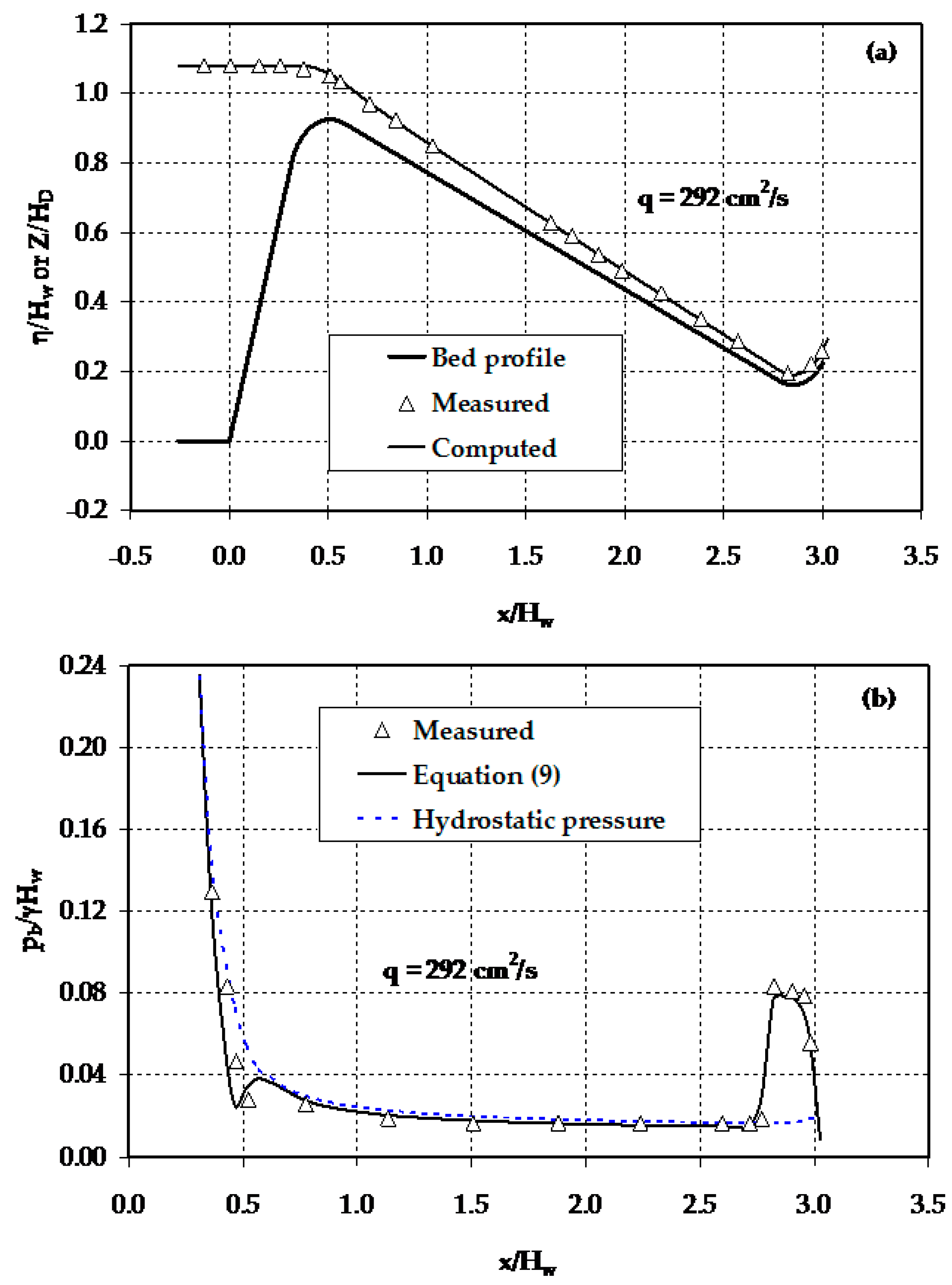
4.1. Non-Hydrostatic Flow over a Spillway

The experiments of this test case were conducted using a horizontal flume with cross-section 464 mm wide and 905 mm high; the length of the flume was 6710 mm. A flip-bucket spillway model with upstream and downstream slopes of 70° and 20°, respectively, was built and installed in the flume. The floor and walls of the model were made of Plexiglass. The spillway crest and the flip bucket were constructed of polyvinyl chloride (PVC) pipe segments with radii 162 mm and 154 mm, respectively and a bucket deflection angle of 45°. The circular-shaped bucket was designed to discharge the jet freely into the air. Under the conditions of the experiment, air entrainment in the supercritical flow was absent. The free-surface elevations along the centreline of the flume were measured to a precision of 0.1 mm using a manual point gauge. Similarly, the pressure on the spillway surface was measured by means of pressure tappings. Despite the small flow rates used in the tests, the results of the experiment were free of scale effects. More details on the experimental system can be found in Khan [28].
The flow problem was simulated by setting up a computational domain that encompassed the entire system of the spillway and the flip bucket, as shown in Figure 2. The flow depth at the inflow section ( j = 0 ) and atmospheric bottom pressure at the end of the free-discharging bucket ( j = m ) were specified as boundary conditions. Figure 3a compares the computed free-surface profile with Khan’s [28] experimental data. In this figure, the dimensionless free-surface elevation, η / H w ( H w is the height of the overflow structure, H D is the flow depth at the upstream end), is shown versus the normalised streamwise horizontal coordinate, x / H w . The numerical result for free-surface profile shows very close agreement with measurement in the subcritical flow region and along the chute of the spillway, where the effects of the streamline vertical curvatures are insignificant. Similar model performance results can be observed over the spillway crest and along the flip bucket. In this flow region, the distribution of the pressure is non-hydrostatic due to the curvilinearity of the streamlines stemming from the curvatures of the circular-shaped spillway crest and flip bucket, as illustrated in Figure 3b. Additionally, the steep free-surface slope of the supercritical flow along the chute plays an important role in modifying the effects of the resistive force in the flow. Subsequently, the pressure distribution departs from hydrostatic (see, e.g., [26,29]) and attains a value of 88.5% of the static pressure. As can be seen from this figure, the bottom pressure rises to a local maximum at x / H w 2.87 and then decreases to atmospheric pressure at the bucket end. Overall, the model accurately mimics the bottom-pressure profile throughout the computational domain. The results of this test depict that the proposed model is capable of resolving the steady rapidly-varied flow problem with continuous free-surface profile to an acceptable degree of accuracy.

4.2. Flow over Trapezoidal-Shaped Weirs

In this section, the predictions of Equation (10a) are compared with the results of Equation (1a) in order to assess the effect of the weakly-curved flow approximation on the performance of the previous equation. As described before, Equation (1a) is a special case of Equation (10a) under the condition of an open channel flow with slightly sloped and curved streamlines. The experimental data of Zerihun [12] and Madadi et al. [30] was selected to validate the numerical results. Zerihun [12] carried out a series of experiments on flow over symmetrical trapezoidal-shaped weirs, made of Plexiglass, with sides sloped at 26.6°, whereas Madadi et al. [30] conducted similar experiments by using unsymmetrical trapezoidal-shaped weirs with upstream side slopes varying from 21° to 90° and a downstream side slope of 54°. The unsymmetrical weir models made of PVC were installed in a flume having glass sidewalls and metal floor. In both experiments, the free-surface elevations along the centreline of the flume were measured by a point gauge of reading accuracy 0.1 mm.
The model boundary conditions employed for these test cases are a specified flow depth and a free-surface slope, which was computed using the gradually-varied flow equation, at the upstream end. The computed free-surface profiles for transcritical flow over a broad-crested weir with an upstream face slope of 21° and a downstream one of 54° are compared with Madadi et al.’s [30] experimental data in Figure 4a. The corresponding relative error, ε , is also shown in Figure 4b. Upstream of the critical section, the two equations give identical results that agree well with measured data. In this region, the effects of a non-hydrostatic pressure distribution and steep free-surface slope are insignificant. Near the downstream edge of the weir crest, the result of Equation (1a) starts to deviate from measurements due to the sharp vertical curvature of the streamline. On the downstream face of the weir, the flow is gradually varied with a steep free-surface slope. Compared to measurements, Equation (1a) predicts flow depths that are too shallow, with a mean relative error of 18% (see Figure 4b). This is due to the fact that this equation does not include terms that account for the effects of a hydraulically steep slope. In contrast, Equation (10a) accurately simulates the free-surface profile throughout the supercritical flow region.
Figure 4c compares the computed free-surface profiles for curvilinear transcritical flow over a short-crested weir with Zerihun’s [12] experimental data. In the upstream subcritical flow region, both equations simulate similar free-surface profile that has an undulatory character. Over the crest of the weir, the free-surface elevation prediction of Equation (1a) slightly deviates from the results of Equation (10a) and the experiment. As can be seen in Figure 4d, the maximum relative errors in the simulation result of these equations are 2.1% and 4%. Downstream of the weir crest, both equations accurately predict the elevations of the free-surface profile. For this moderately sloped problem, the performance of both equations is satisfactory and the results are indistinguishable except over the weir crest.
The results of the above test cases demonstrate that applying the simplifying assumption of small streamline inclination and curvature gives a simpler and less accurate hydrodynamic equation for curved flows in steeply sloping channels. Nonetheless, it is preferable to employ the more complicated Equation (10a), which has performed well on moderate and steep slopes flow problems involving curvilinear effects.

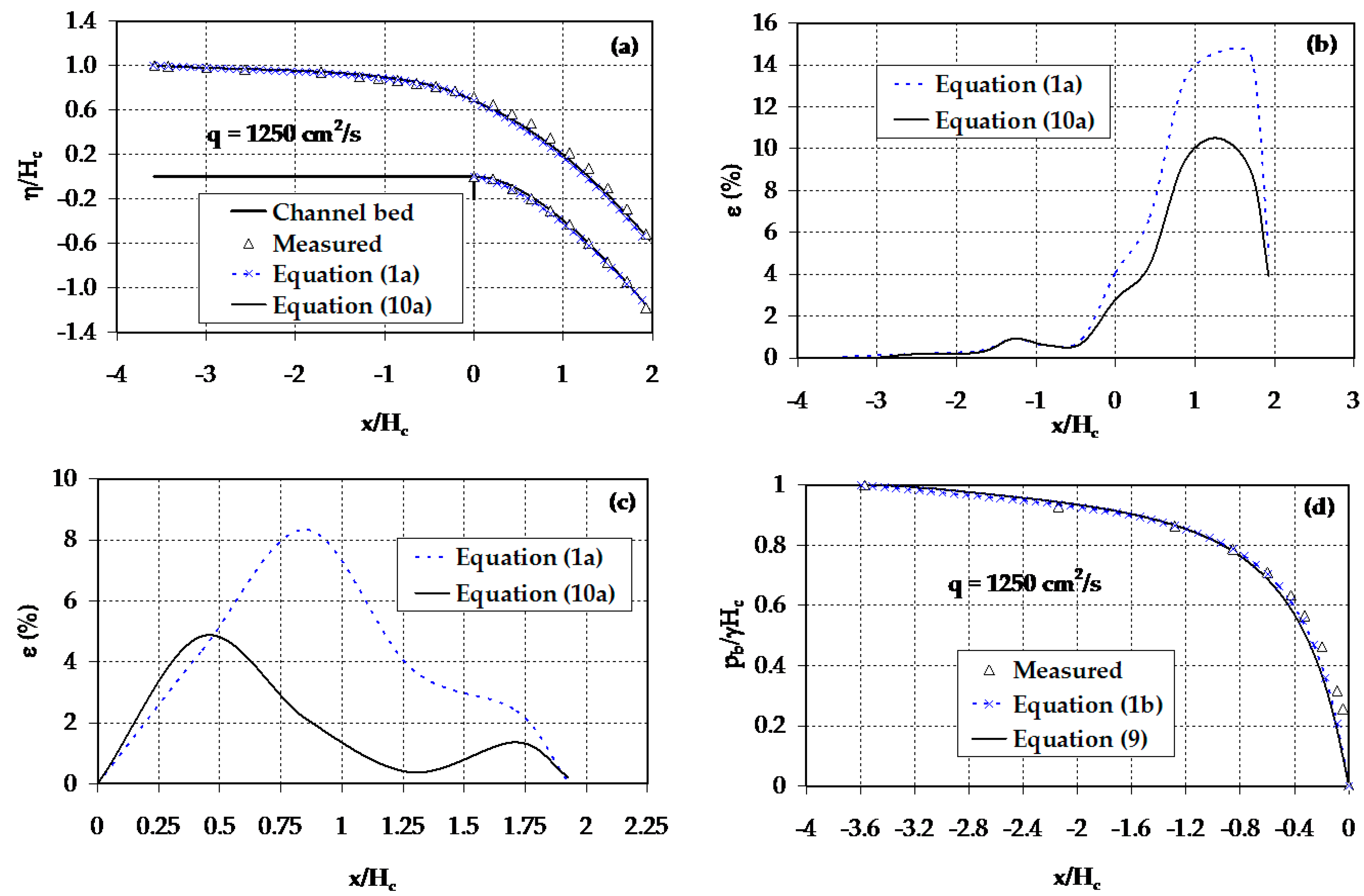
4.3. Curvilinear Overfalls

The feasibility of the proposed model and Fawer’s [7] equations was further examined by modelling curvilinear flow with dual free-surfaces such as a rectangular free overfall. Such a flow problem can be simulated by treating the fixed bed and the free jet portion of the flow as a single flow problem and then applying both the flow profile and pressure equations. Figure 5 presents a schematic diagram of the free overfall. For the free jet portion, the pressure at the underside of the nappe is atmospheric. Using this known auxiliary boundary condition, the following discretised equation for the elevation of the lower nappe of the jet, Z , is obtained from the bottom-pressure equation:
( Z j 1 2 Z j + Z j + 1 ) ( ω 2 , j + 1 ω 1 , j ω 2 , j ) + ( 2 g H j 2 ω 1 , j q 2 ( Δ x ) 2 + 1 ω 1 , j ( H j 1 2 H j + H j + 1 ) ) = 0
At the downstream end ( j = m ), the elevation of the lower nappe was specified as an outflow boundary condition for the solution of the free-surface profile of this nappe. Similarly, the discretised form of Equation (13), together with the specified flow depth and atmospheric bottom pressure at the upstream end ( j = 0 ) and brink section, respectively, was solved numerically to model the upper free-surface profile.
The above numerical procedure for the solution of the proposed model provides a convenient method of developing a discharge rating curve for free overfall with subcritical approach flow and overcomes the drawbacks of the theoretical methods based on simplifying assumptions or empirical relations originating from measurements.
The computed free-surface and bottom-pressure profiles for subcritical approach flow are compared with Rouse’s [31] experimental data. The experiments were performed in a horizontal, rectangular and smooth channel. The floor and sidewall of the channel were constructed from smooth concrete. The free-surface elevations and the bottom-pressure profile were measured, respectively, by point and hook gauges and piezometers. The uncertainty in the free-surface measurements was ±0.1 mm. Figure 6a shows the variation of the normalised free-surface elevation, η / H c ( H c ( = q 2 / g 3 ) is the critical depth), with the normalised streamwise horizontal coordinate, x / H c . Upstream of the brink section, the results of Equations (1a) and (10a) show very close agreement with experimental data. It can be seen from Figure 6a that the computational results of Equation (10a) for the lower- and upper-nappe profiles of the jet correspond well with experimental data. Similar to the previous test cases, the results of Equation (1a) for these profiles slightly depart from measurements. This numerical experiment indicates that Equation (10a) is capable of simulating accurately the free overfall problem with subcritical inflow condition irrespective of the sharp vertical curvatures of the streamline. For subcritical inflow condition, the flow depth at the brink section is an important parameter for estimating the discharge. Both equations predict this depth satisfactorily with relative errors of 3% and 4%, as shown in Figure 6a,b.
Figure 6d shows the results of Equations (1b) and (9) for the bottom-pressure profile upstream of the brink section. In this figure, the non-dimensional bottom pressure at any section, p b / γ H c , is shown versus the normalised streamwise horizontal coordinate, x / H c . As can be seen from this figure, the predicted results compare well with experimental data. The mean relative errors in the numerical result of Equations (1b) and (9) are 3.4% and 4.2%, respectively.

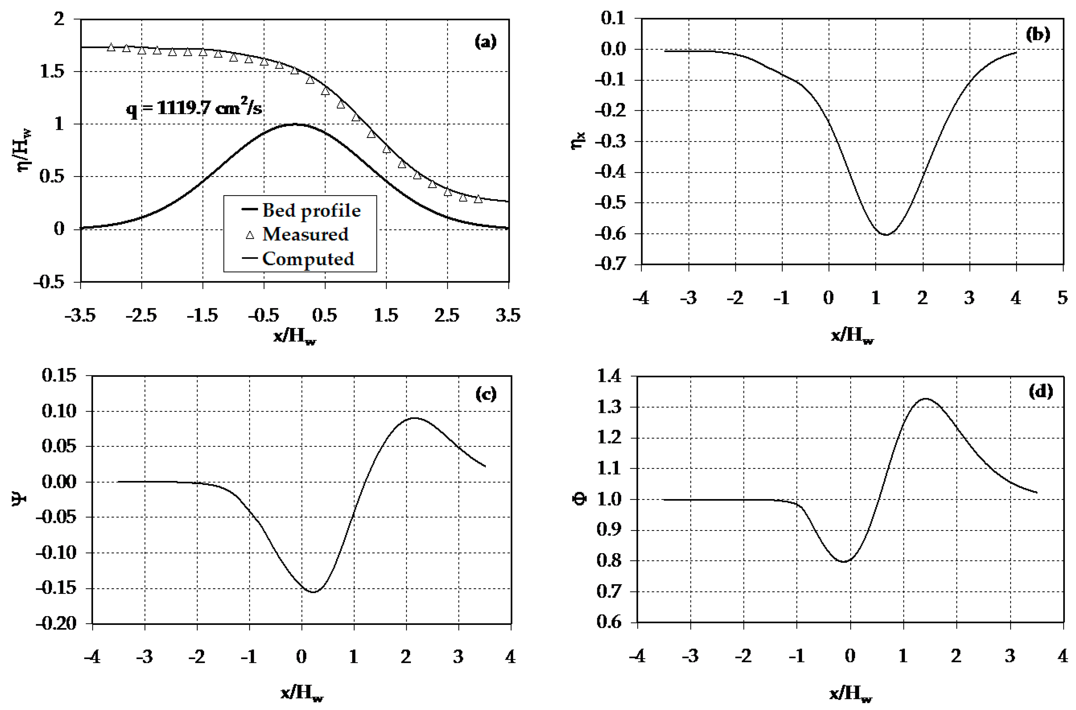
4.4. Nature of the Higher-Order Curvature Terms

The equation of the non-hydrostatic depth-averaged model, Equation (10a), may be expressed as
E = H ω 1 + q 2 2 g H 2 Φ
where Φ is the depth-averaged correction coefficient for the dynamic effects of the vertical acceleration. This coefficient may reach a value greater or lower than 1.0, depending on the slope and vertical curvature of the streamline. For a quasi-uniform flow situation, Φ is very close to unity. Based on the numerical results of Equation (10a), the variations of the correction coefficient, free-surface slope and curvature along the streamwise horizontal distance are investigated for a non-hydrostatic flow problem. It is apparent that the degree of approximation for these terms strongly influences the overall quality of the simulation results of the extended energy equation. One of the experimental results of Sivakumaran [32] for curved flow over a hump was invoked to verify the contribution of the terms. These experiments were conducted in a horizontal flume 9150 mm long, 650 mm deep and 300 mm wide. The flume was made of a steel frame with glass windows on both sides and its floor was constructed from plywood. A symmetrical hump made of PVC was tested, among others. The free-surface profile along the centreline of the hump was measured using a point gauge of reading accuracy 0.10 mm.
As in the test case of flow over a trapezoidal-shaped weir, the flow depth and the free-surface slope were specified as inflow boundary conditions. Figure 7a compares the numerical result for free-surface profile with Sivakumaran’s [32] experimental data. As shown in this figure, the simulated free-surface profile shows good agreement with the experiment data. The variations of the free-surface slope, η x and the relative curvature, Ψ ( = η x x H / ω 1 3 / 2 ) , are plotted in Figure 7b,c, respectively. It can be seen from this figure that the slope and curvature of the free-surface attain maximum values at a section just downstream from the crest of the hump. As described before, the flow field of this region is characterised by a departure from the hydrostatic pressure distribution due to the effects of the vertical acceleration. In the vicinity of the inflow and outflow sections, the flow is nearly horizontal with parallel streamlines. Consequently, the contributions of these two terms are negligible. The computational result for the depth-averaged correction coefficient is depicted in Figure 7d. As shown in this figure, the local maximum values of this correction coefficient occur in the curvilinear flow region where the streamlines are moderately sloped and sharply curved. Furthermore, the profile of the correction coefficient follows a similar trend to the simulated values of the relative free-surface curvature term. It is obvious from Figure 7c,d that for convex free-surface flow, Ψ < 0 which corresponds to Φ < 1.0 . The opposite is true for the case of concave flow. All these facts demonstrate that the magnitude of the correction coefficient depends mainly on the relative curvature of the flow, more weakly on the free-surface slope. The foregoing discussion highlights the importance of the higher-order curvature terms and their contribution to the correction coefficient term in Equation (17).
For all flow problems, in which both strong streamline vertical curvatures and steep slopes prevail, the free-surface and bottom-pressure profiles were simulated reasonably well by the proposed steep-slope form of the non-hydrostatic depth-averaged model. The overall comparison results revealed that such a type of model is suitable for analysing curvilinear flow problems with continuous free-surface profiles in steeply sloping channels. For other types of problems where turbulence effects are important such as rapidly-varied flows with discontinuous free-surface profiles, curvilinear flow models based on a momentum approach are appropriate to investigate the problems. The outcomes of this work are pertinent to discharge measurements in open channel systems which are commonly carried out by constructing flow-measuring structures of various geometric shapes. In the following section, higher-order critical flow conditions based on the current model will be developed and applied to simulate the discharge characteristics of a round-crested weir. It is important to note that the selected experimental data for verifying the proposed method is free of surface tension and viscosity effects.

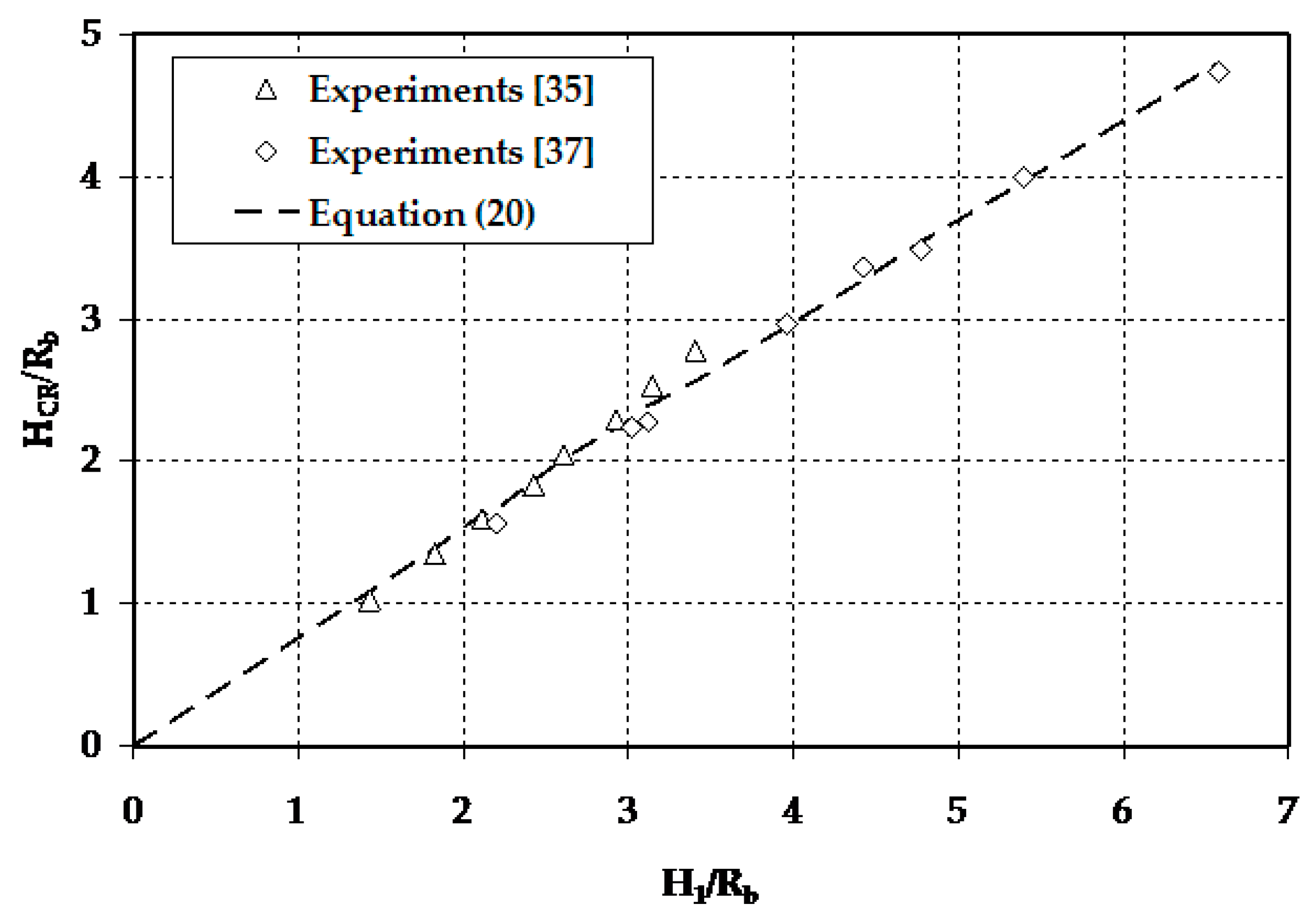
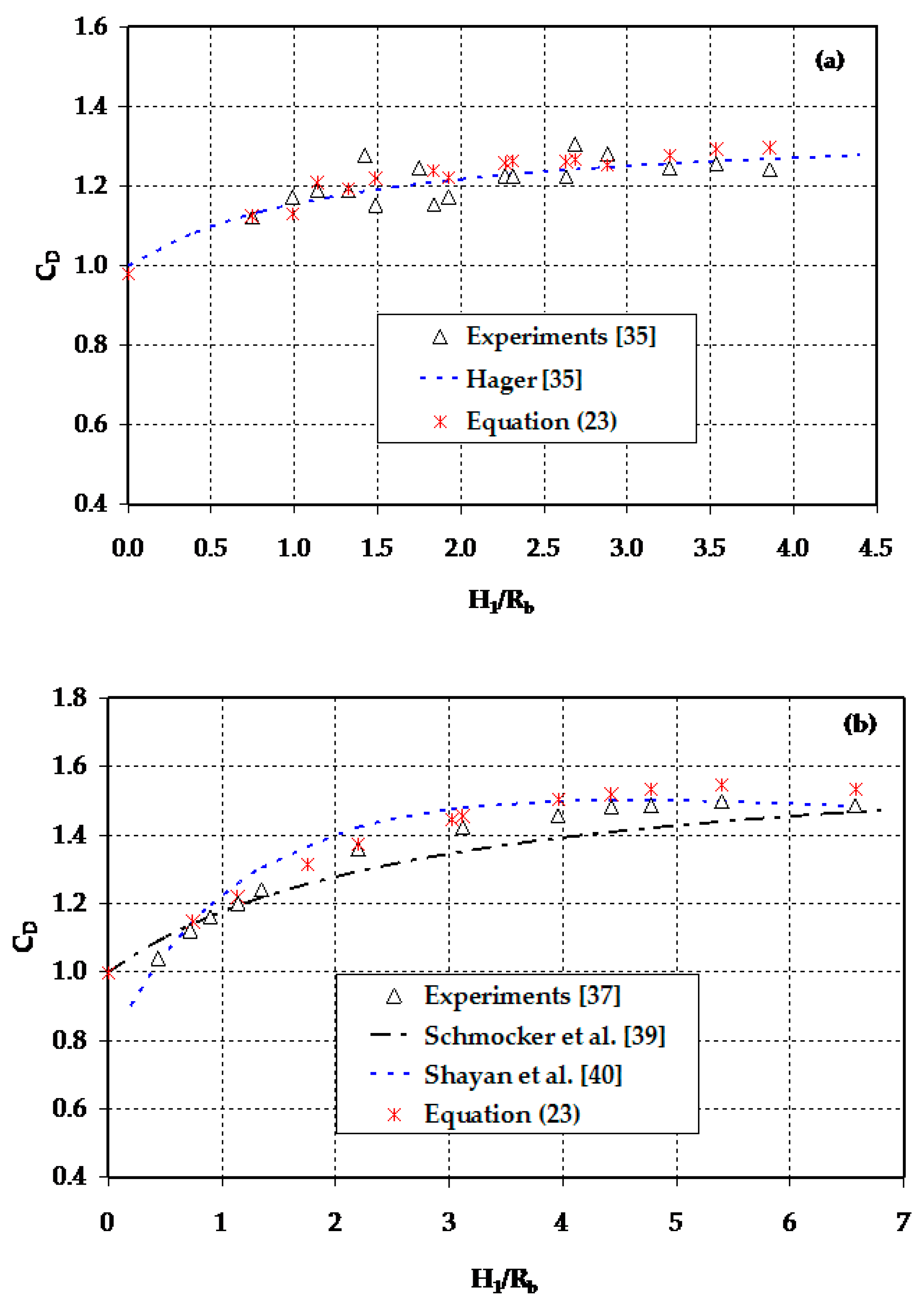
5. Critical Flow Conditions in Curvilinear Free-Surface Flows

Critical flow is an intermediate flow state between subcritical and supercritical flows in which the specific energy attains a minimum value for a constant discharge or conversely, it is a flow state corresponding to a maximum discharge for a constant specific energy head [22]. In practice, the critical flow section serves as a control section for establishing a unique relationship between the flow depth and discharge. The precise location of such a control section is dependent on the shape of the artificial control structures such as a weir. As pointed out by Jaeger [18], conditions of critical flow can occur in the immediate neighbourhood of the maximum bottom elevation. Using such conditions for a round-crested weir flow problem, the relationship between the minimum specific energy ( E = H e Z ) and the critical depth can be obtained by differentiating Equation (10a) with respect to H , while the discharge remains constant ( Z x 0 and ω 2 = 1 ).
d E d H = 1 q 2 g H C R 2 Γ 1 q 2 g H C R 3 Γ 2 = 0
Γ 1 = H x x 3 + Z x x 2 = ( 2 R b ω 1 3 / 2 + R s 6 R b R s )
Γ 2 = ω 1 ( α + ( H x ) 2 3 )
where R b and R s are the radii of curvature of the bed and the free-surface streamline, respectively; and H C R is the crest or the critical flow depth. In the absence of measured data, the radius of the free-surface streamline at the crest can be estimated by [7,18]
R s R b + ω 0 H C R
where ω 0 is a distribution parameter. Based on Fawer’s experimental data for free flow over a circular-crested weir, Jaeger [18] suggested a value of 2.0 for ω 0 . Equation (18a) is a higher-order equation for critical depth, which accounts for the effects of the streamline vertical curvature. If the geometric characteristics of the free-surface streamline at a critical section are known in addition to the flow parameters, one can use this equation to predict the critical depth and then the minimum specific energy for curvilinear critical flow situations. For a particular case of critical section with a quasi-uniform flow condition ( Γ 1 = 0 and Γ 2 = 1 ), Equation (18a) simplifies to
q 2 g H C R 3 = 1
As highlighted above, a simplified critical flow approach for flow with curved streamlines can provide useful solutions for practical flow problems with a fixed channel section for a critical depth computation. For the case of free-surface flow over a round-crested weir, Equation (18a) can be rewritten as
H C R 3 q 2 Γ 1 g H C R q 2 g Γ 2 = 0
In the above equation, Γ 2 is always positive. However, the sign of Γ 1 depends on the shape of the streamline curvature. In the case of convex open-channel flows such as free flows over a round-crested weir, Γ 1 is always negative. For such flows, Equation (20) has only one real-valued positive root for the crest flow depth and can be deduced by the Picard iteration technique. Previous studies by Bos [33] and Ramamurthy et al. [34] show that the ratio of this depth to the upstream crest-referenced energy head takes a nearly constant value of approximately 0.72 for a circular-crested weir with upstream and downstream face slopes being 90° and 45°, respectively. Using the flow depth at the weir crest, the specific energy of the flow at this section, E C R , can be deduced from Equation (10a), i.e.,
E C R = q 2 ω 1 g H C R Γ 1 + q 2 2 ω 1 g H C R 2 Γ 2 + H C R ω 1
For steady flow past an overflow structure, the discharge can be expressed as a function of the upstream crest-referenced energy head, H 1 , as [33]
q = C D 2 3 3 2 g H 1 3 / 2
where C D is the discharge coefficient. Accurate determination of the discharge characteristics of a round-crested weir requires the application of a hydrodynamic equation that accounts for the effects of a non-hydrostatic pressure distribution. The combination of Equations (21) and (22) yields an expression for the discharge coefficient as
C D = 3 3 2 H C R H 1 3 / 2 ( ω 1 E C R H C R 2 H C R Γ 1 + Γ 2 ) 1 / 2
As described by Bos [33], this coefficient takes into account the effects of the streamline vertical curvature over the crest of such a short-crested type of weir. For modelling the head-discharge characteristics, E C R is estimated from the upstream crest-referenced head by considering head losses between the crest section and the upstream gauging station. It is evident that the lowest-order approximate equation can be recovered from Equation (23) for the case of free-surface flows with parallel-streamlines. Compared to earlier method by Hager [35], the present method is not restricted to flow situations with weakly inclined and curved streamlines. It also differs from the Ramamurthy and Vo [36] potential-flow approach in which the critical flow conditions were not imposed.
The computed crest flow depths and discharge coefficients are compared with experimental data of Hager [35] and Vo [37]. Hager [35] conducted experimental studies for flows over cylindrical weirs with radii 44 mm, 57 mm and 90.2 mm. In an analogous manner, Vo [37] carried out detailed experimental investigations for examining the features of a free flow over circular-crested weirs. He tested weir models having different radii and face slopes. Test results of weirs with a vertical upstream face and downstream face slopes of 45° and 60° were selected to validate the proposed method. In both experiments, the free-surface profiles and velocity distributions were measured for different discharges. As shown in Figure 8, the validation result indicates a good correlation between the numerical and experimental data for the crest flow depth. Similar to the brink section of a free overfall, the crest section of a circular-crested weir can serve as a control section for establishing head-discharge relationships by applying experimental and numerical methods in conjunction with the theory of critical flow, or without resorting to this theory (see, e.g., [21,34,35,37,38]).
Figure 9 provides a comparison of the current method results with the results of semi-empirical equations proposed by Hager [35], Schmocker et al. [39] and Shayan et al. [40]. The numerical results of the present method for discharge coefficient compare favourably with experimental data (mean relative error of less than 5%) and are slightly better than the results of these equations. For the range of flow considered here ( H 1 / R b < 7 ), the discharge coefficient increases with increasing the relative crest curvature, H 1 / R b . This is due to the effects of the gradual increase of the streamline vertical curvature over the weir crest. As noted by Ramamurthy and Vo [41], a circular-crested weir acts like a sharp-crested weir when H 1 / R b and attains its limiting discharge coefficient value. It is apparent that the streamline curvature over the weir crest becomes negligible as R b . Consequently, C D approaches to the theoretical value of 1.0, as depicted in this figure. The overall simulation results of the round-crested weir flow problem demonstrate that the proposed method is efficient and accurate in modelling the discharge characteristics of non-hydrostatic flows over such a type of weir.

6. Conclusions

This study extended the depth-averaged energy model by including not only the effects of the dynamic pressure but also the effect of steep free-surface slope, which makes the current model entirely different from the previous Boussinesq-type energy models (e.g., [7,8,10]). Besides, the potential-flow theory, which is the basis of these models, was not employed to develop the new model. An implicit scheme of finite differences was implemented to discretise and solve the model equation. The model was then applied to simulate rapidly-varied flow problems with continuous free-surface profiles and its results were compared to experimental data and the results of earlier higher-order model and semi-empirical equations.
For all test cases, the proposed model accurately predicted the free-surface and bottom-pressure profiles irrespective of the vertical curvature of the streamline, demonstrating its capacity for handling flow situations with strong curvilinear effects. Analyses of the comparison results showed that the weakly-curved flow approximation did not have a significant impact on the results of Equation (1a) for a non-hydrostatic free-surface flow in a moderately sloping channel. For the case of curved-streamline flow in a steep-slope channel, however, results from this equation were not quite so accurate. This is due to the fact that Equation (1a) does not have terms that account for the effects of a hydraulically steep slope. Although the present model is relatively complex, the significance of the terms was clearly seen from the model comparison results, particularly for curvilinear supercritical flows in a steeply sloping channel. The increase of computational effort of this model over the weakly-curved flow formulation is reasonably small.
As part of the study, a numerical approach based on the theory of curvilinear critical flow was developed to compute the free-flow discharge coefficient for round-crested weirs. The method was demonstrated to provide reasonably accurate discharge coefficients for such types of weirs under free-flow conditions, with a mean relative error of less than 5%. It also overcame the limitations of the conventional theory of critical flow, which is only applicable to open channel flows with parallel-streamlines. The proposed method has a potential to be extended and applied as a computational tool for analysing the head-discharge characteristics of other types of short-crested weirs to a satisfactory degree of approximation.

Acknowledgments

The author would like to express his sincere appreciations to the anonymous reviewers for their valuable comments and suggestions.

Conflicts of Interest

The author declares no conflict of interest.

References

  1. Savage, S.B.; Hutter, K. The motion of a finite mass of granular material down a rough incline. J. Fluid Mech. 1989, 199, 177–215. [Google Scholar] [CrossRef]
  2. Berger, R.C. Free-Surface Flow over Curved Surfaces. Ph.D. Thesis, University of Texas, Austin, TX, USA, 1992. [Google Scholar]
  3. Berger, R.C.; Carey, G.F. Free-surface flow over curved surfaces-Part I: Perturbation analysis. Int. J. Numer. Method Fluids 1998, 28, 191–200. [Google Scholar] [CrossRef]
  4. Berger, R.C. Strengths and weaknesses of shallow-water equations in steep open channel flow. In Proceedings of the National Conference on Hydraulic Engineering, ASCE, Buffalo, NY, USA, 1–5 August 1994; Volume 2, pp. 1257–1262. [Google Scholar]
  5. Keller, J.B. Shallow-water theory for arbitrary slopes of the bottom. J. Fluid Mech. 2003, 489, 345–348. [Google Scholar] [CrossRef]
  6. Denlinger, R.P.; O’Connell, D.R. Computing non-hydrostatic shallow-water flow over steep terrain. J. Hydraul. Eng. 2008, 134, 1590–1602. [Google Scholar] [CrossRef]
  7. Fawer, C. Etude de Quelques Écoulements Permanents à Filets Courbes (Study of Some Permanent Flows with Curved Filaments). Docteur ès Sciences Techniques Thèse, Université de Lausanne: Lausanne, Switzerland, 1937. (In French) [Google Scholar] [CrossRef]
  8. Hager, W.H.; Hutter, K. Approximate treatment of plane channel flow. Acta Mech. 1984, 51, 31–48. [Google Scholar] [CrossRef]
  9. Hager, W.H. Equations for plane, moderately curved open channel flows. J. Hydraul. Eng. 1985, 111, 541–546. [Google Scholar] [CrossRef]
  10. Matthew, G.D. Higher-order, one-dimensional equations of potential flow in open channels. Proc. Inst. Civ. Eng. 1991, 91, 187–201. [Google Scholar] [CrossRef]
  11. Castro-Orgaz, O.; Hager, W.H. One-dimensional modelling of curvilinear free-surface flow: Generalised Matthew theory. J. Hydraul. Res. 2014, 52, 14–23. [Google Scholar] [CrossRef]
  12. Zerihun, Y.T. A One-Dimensional Boussinesq-Type Momentum Model for Steady Rapidly-Varied Open Channel Flows. Ph.D. Thesis, Department of Civil and Environmental Engineering, The University of Melbourne, Melbourne, VIC, Australia, 2004. [Google Scholar]
  13. Benjamin, T.B.; Lighthill, M.J. On cnoidal waves and bores. Proc. R. Soc. A 1954, 224, 448–460. [Google Scholar] [CrossRef]
  14. Marchi, E. The nappe profile of a free overfall. Rend. Mat. Acc. Lincei. 1992, 3, 131–140. [Google Scholar]
  15. Marchi, E. On the free overfall. J. Hydraul. Res. 1993, 31, 777–790. [Google Scholar] [CrossRef]
  16. Castro-Orgaz, O.; Giráldez, J.V.; Ayuso, J.L. Higher-order critical flow condition in curved-streamline flow. J. Hydraul. Res., 2008, 46, 849–853. [Google Scholar] [CrossRef]
  17. Dressler, R.F. New nonlinear shallow flow equations with curvature. J. Hydraul. Res. 1978, 16, 205–220. [Google Scholar] [CrossRef]
  18. Jaeger, C. Engineering Fluid Mechanics; Blackie and Son Limited: London, UK; Glasgow, UK, 1956; pp. 65–135. [Google Scholar]
  19. Liggett, J.A. Critical depth, velocity profile and averaging. J. Irrig. Drain. Eng. 1993, 119, 416–422. [Google Scholar] [CrossRef]
  20. Chanson, H. Minimum specific energy and critical flow conditions in open channels. J. Irrig. Drain. Eng. 2006, 132, 498–502. [Google Scholar] [CrossRef]
  21. Castro-Orgaz, O.; Chanson, H. Depth-averaged specific energy in open-channel flow and analytical solution for critical irrotational flow over weirs. J. Irrig. Drain. Eng. 2014, 140. [Google Scholar] [CrossRef]
  22. Rouse, H. Fluid Mechanics for Hydraulic Engineers; McGraw-Hill: New York, NY, USA, 1938; pp. 51–284. [Google Scholar]
  23. Serre, F. Contribution à l’étude des écoulements permanents et variables dans les canaux (Contribution to the study of permanent and nonpermanent flows in channels). La Houille Blanche 1953, 8, 374–388. (In French) [Google Scholar] [CrossRef]
  24. Yuan, S.W. Foundations of Fluid Mechanics; Prince Hall International, Inc.: Eaglewood Cliffs, NJ, USA, 1988; p. 149. [Google Scholar]
  25. White, F.M. Fluid Mechanics, 7th ed.; McGraw-Hill: New York, NY, USA, 2011; p. 280. [Google Scholar]
  26. Chaudhry, M.H. Open Channel Flow, 2nd ed.; Springer and Media Science LLC: New York, NY, USA, 2008; pp. 18–37. [Google Scholar]
  27. Abramowitz, M.; Stegun, I.A. Handbook of Mathematical Functions with Formulas, Graphs and Mathematical Tables, 10th ed.; Wiley: New York, NY, USA, 1972; p. 877. [Google Scholar]
  28. Khan, A. Modelling Rapidly-varied Open Channel Flows. Ph.D. Thesis, Department of Civil Engineering, University of Alberta, Edmonton, AB, Canada, 1995. [Google Scholar]
  29. Chow, V.T. Open-Channel Hydraulics; McGraw-Hill: New York, NY, USA, 1959; pp. 32–33. [Google Scholar]
  30. Madadi, M.R.; Dalir, A.H.; Farsadizadeh, D. Investigation of flow characteristics above trapezoidal broad-crested weirs. Flow Meas. Instrum. 2014, 38, 139–148. [Google Scholar] [CrossRef]
  31. Rouse, H. The Distribution of Hydraulic Energy in Weir Flow in Relation to Spillway Design. Master’s Thesis, Massachusetts Institute of Technology, Boston, MA, USA, 1932. [Google Scholar]
  32. Sivakumaran, N.S. Shallow Flow over Curved Beds. DEng Thesis, Asian Institute of Technology, Bangkok, Thailand, 1981. [Google Scholar]
  33. Bos, M.G. Discharge Measurement Structures, 3rd ed.; International Institute for Land Reclamation and Improvement: Wageningen, The Netherlands, 1989; pp. 40–202. [Google Scholar]
  34. Ramamurthy, A.S.; Vo, N.D.; Vera, G. Momentum model of flow past a weir. J. Irrig. Drain. Eng. 1992, 118, 988–994. [Google Scholar] [CrossRef]
  35. Hager, W.H. Critical flow condition in open-channel hydraulics. Acta Mech. 1985, 54, 157–179. [Google Scholar] [CrossRef]
  36. Ramamurthy, A.S.; Vo, N.D. Application of Dressler theory to weir flow. J. Appl. Mech. 1993, 60, 163–166. [Google Scholar] [CrossRef]
  37. Vo, N.D. Characteristics of Curvilinear Flow past Circular-Crested Weirs. Ph.D. Thesis, Concordia University, Montreal, QC, Canada, 1992. [Google Scholar]
  38. Chanson, H.; Montes, J.S. Overflow Characteristics of Cylindrical Weirs; Research Report No. CE154; Department of Civil Engineering, University of Queensland: Brisbane, QLD, Australia, 1997. [Google Scholar]
  39. Schmocker, L.; Halldórsdóttir, B.R.; Hager, W.H. Effect of weir face angles on circular-crested weir flow. J. Hydraul. Eng. 2011, 137, 637–643. [Google Scholar] [CrossRef]
  40. Shayan, H.K.; Khezerloo, A.B.; Farhoudi, J.; Aminpoor, Y. A discussion to “Discharge coefficient of circular-crested weirs based on a combination of flow around a cylinder and circulation”. J. Irrig. Drain. Eng. 2015, 141. [Google Scholar] [CrossRef]
  41. Ramamurthy, A.S.; Vo, N.D. Characteristics of circular-crested weir. J. Hydraul. Eng. 1993, 119, 1055–1062. [Google Scholar] [CrossRef]
Figure 1. Definition sketch for free-surface flow with curved streamlines.
Fluids 02 00049 g001
Figure 2. Definition sketch and computational domain for the spillway flow problem.
Fluids 02 00049 g002
Figure 3. Curvilinear transcritical flow over a spillway with sharply-curved crest and flip bucket: (a) free-surface profile; (b) bottom-pressure profile.
Fluids 02 00049 g003
Figure 4. (a) Free-surface profile for transcritical flow over a broad-crested weir with a steep downstream face slope; (b) comparison of relative errors; (c) free-surface profile for curvilinear transcritical flow over a short-crested weir with moderate face slopes; (d) comparison of relative errors.
Fluids 02 00049 g004
Figure 5. Definition sketch and computational domain for the free overfall problem.
Fluids 02 00049 g005
Figure 6. Curvilinear overfall with subcritical approach flow: (a) free-surface profile; (b) comparison of relative errors for the upper free-surface profile result; (c) comparison of relative errors for the lower-nappe profile result; (d) bottom-pressure profile.
Fluids 02 00049 g006
Figure 7. Curved-streamline flow over a hump: (a) free-surface profile; (b) free-surface slope; (c) relative curvature of the free-surface; (d) correction coefficient for the vertical acceleration effects.
Fluids 02 00049 g007
Figure 8. Variation of the crest flow depth with the relative crest curvature, H 1 / R b .
Fluids 02 00049 g008
Figure 9. Free-flow discharge coefficients for two different types of round-crested weirs: (a) cylindrical weirs; (b) circular-crested weirs.
Fluids 02 00049 g009

