
Anisotropic Wave Turbulence for Reduced Hydrodynamics with Rotationally Constrained Slow Inertial Waves


Abstract
:1. Introduction
2. Reduced-Rotating Hydro-Dynamic Equations, R-RHD
2.1. Geostrophic Inertial Waves and Eddies
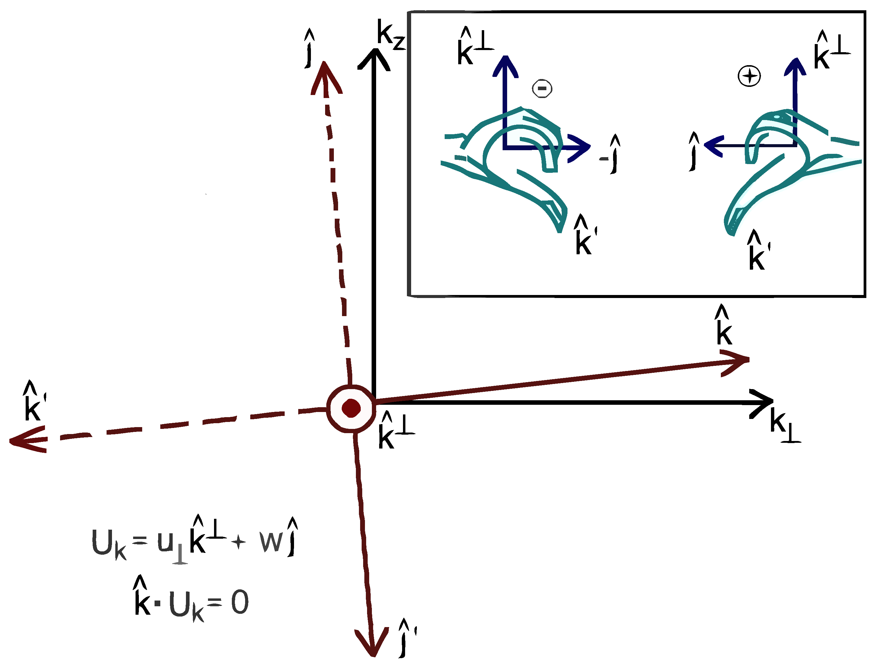
2.2. Helical Basis for Circularly Polarized Inertial Waves
3. Dynamical Limits of Turbulence and Multiple Scales Order Parameters
3.1. Time Period of Oscillations of Waves and Amplitudes
3.2. Notations and New Slow Time Variables for the Multiple Scales Derivation Presented in This Paper
- : slow time scale of weak amplitudes (slowest time scale),
- : slow R-RHD wave time scale, and
- : fast inertial wave time scale (filtered out by R-RHD).
3.3. Definitions of Turbulence Regimes
- WT:
- .
- AT:
- . In essence, one may envision the AT dynamical regime for hydrodynamics as a zoomed in version of the WT limit in Galtier [8]. In this paper we investigate the subtle variations in the flow dynamic at this magnified scale concealed by the treatment in [8]. Further, in this paper, we perform the multiple scales analysis in the anisotropic regime defined by the order parameter . So the region of validity of AT is also set by the limit where .
- CB:
- .
4. Wave Amplitude Equations
4.1. Dimensional Consistency of Wave Amplitude Equation (22)
4.2. Spectral Tensor
5. Zero Helicity Dynamics
5.1. The Hamiltonian
5.2. Kinetic Equations
5.2.1. Closure

5.2.2. Dimensional Consistency of the kinetic Equation (43)
5.2.3. Physical Realizability of Spectrum Prescribed by Equation (43) and Comparison with Quasi-Normal Type Closures
5.2.4. Invariants of the Closed Kinetic Equations
5.2.5. Kolmogorov Solution of the Kinetic Equations
- (i)
- and (Rayleigh-Jeans (RJ) spectrum).
- (ii)
- and .
- (iii)
- and , where and are respectively the powers of and in . Clearly, in our case, . Thus, and .
- (iv)
- and . This solution corresponds to the constant flux in the z-component of the momentum.
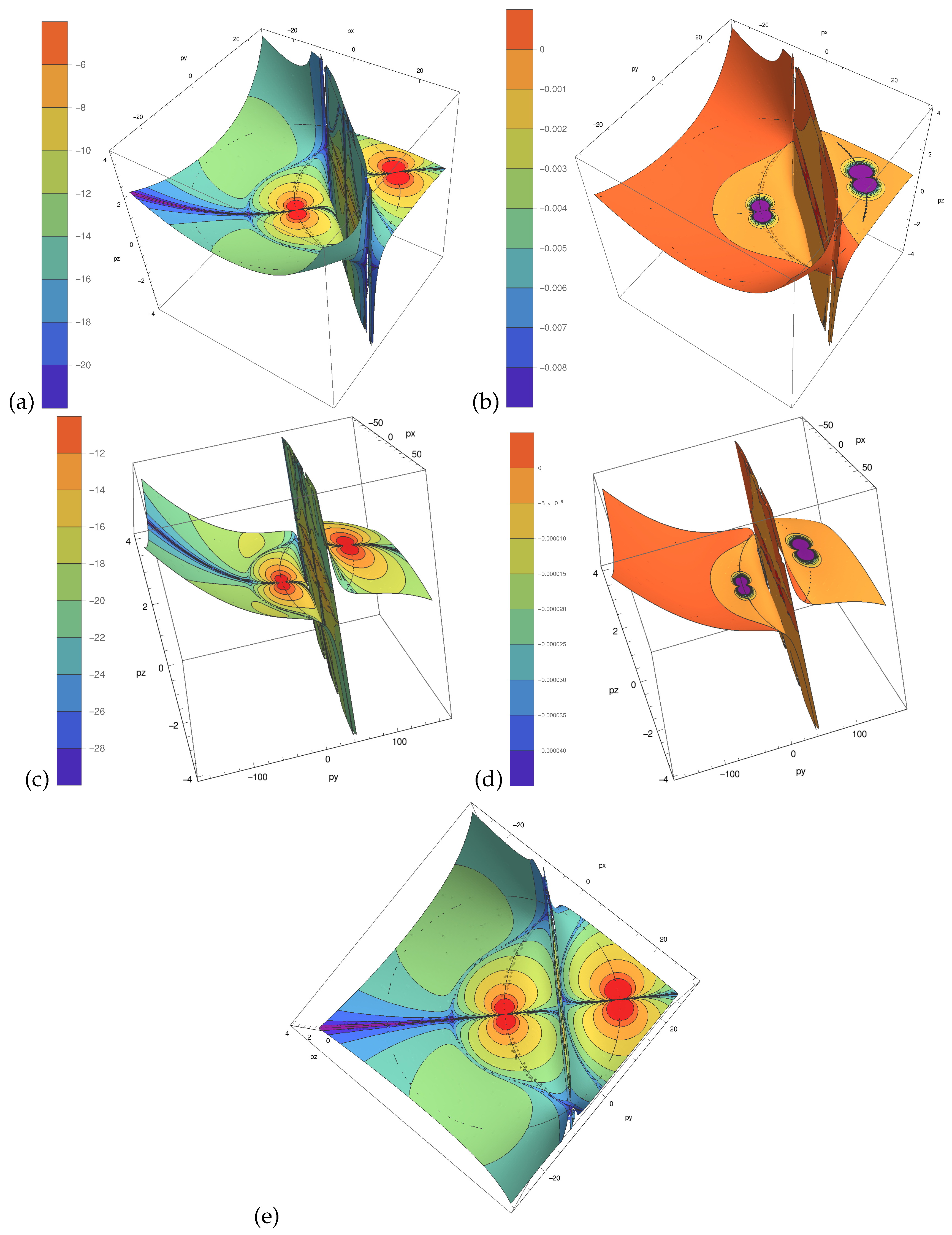
5.2.6. Locality of Interactions and Convergence of Collision Integral
6. Non-Zero Helicity Dynamics: Interplay of Energy and Helicity
6.1. Coupled Equations for Energy and Helicity
6.2. Generalized Solution of Energy and Helicity Spectra
6.3. Hierarchy of Slow Manifolds in Anisotropic Wave Turbulence Diverges from the Critical Balance Route towards Isotropy
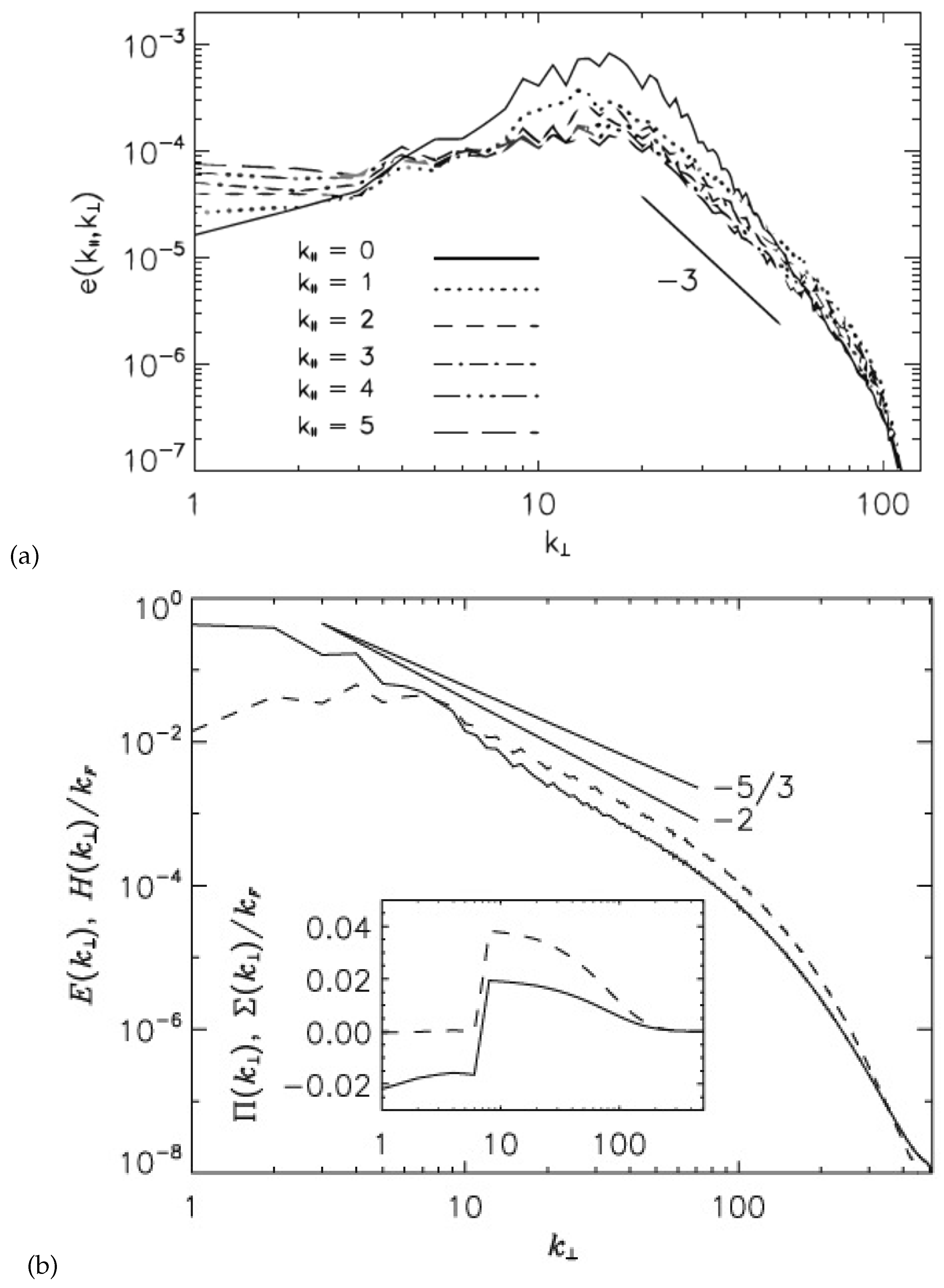
6.4. Comparison with Weak Turbulence Theory of Galtier
- The governing equations on which the wave turbulence theory [8,9] is developed are the Navier-Stokes equations (i.e., Equation (1)). In these equations, the Rossby number appears explicitly and is used as an order parameter in the perturbation analysis and the fast inertial wave dynamic is dominant. In contrast, the governing equations for the analysis presented here are the R-RHD (i.e., Equations (5) and (6)). The asymptotic limit of infinitesimally small is already accounted for in the multiple scales analysis to derive the R-RHD and hence do not explicitly appear in the R-RHD equations. This means that the effect of fast inertial waves is sub-dominant here and the R-RHD equations are hence suitably applicable for the slow manifold dynamics.
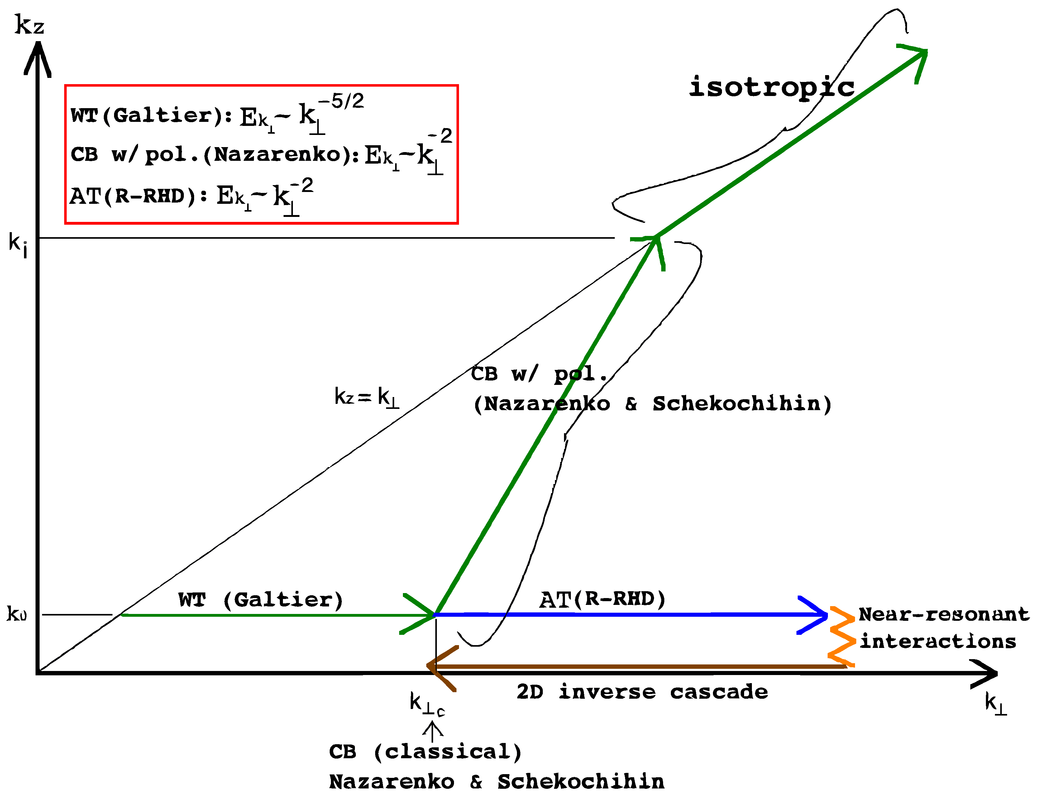
- The dynamical regime where the theory [8,9] is valid is . This point has been elaborated in great detail in the work of Nazarenko and Scheckochihin [27] (see Section 2 in [27]). The dynamical regime of the R-RHD is and . It is the limit in which is so small that the turbulent dynamic is populated by slow inertial waves with dispersion relation embodying slow oscillations when (also see Figure 5 above). In other words, within the slow manifold, is so small that . The perturbative analysis presented here is applied to the R-RHD where the smallness (weakness) of the wave amplitude is measured by and the slow dispersive three wave system undergoes weak non-linear exchanges at the asymptotic order as explained earlier in Section 4 and Section 5.
- In wave turbulence theory of Galtier [8] and Galtier [9], the kinetic equations for energy and helicity are derived by using multiple correlation functions to capture the energetics as well as the absence of symmetry due to helicity. This makes the calculations tediously lengthy. In contrast, the derivation for the helicity kinetic equation is presented here as a natural extension of the symmetrical non-helical system and bypasses the use of calculations using multiple correlation functions. This simpler approach follows a more general philosophy of Hamiltonian reduction exploiting symmetries in the system [25] and their natural extension to understanding asymmetrical phenomena.
- Finally, the spectral power laws obtained for the energy cascade are distinctly different as explained concisely in Figure 5.
6.5. Comparison with Weak Turbulence Theory of Newell: Cumulant Hierarchy vs. Wave Amplitude Hierarchy
7. Coupling between Wave and 2D Modes Through Non-Resonant Interactions
8. Conclusions
Acknowledgments
Conflicts of Interest
Appendix A
Appendix A.1. Notations and Definitions of Wave Vectors and Gradient Operators
Appendix A.2. Derivation of the Amplitude Equation: Supplementary Calculations
Appendix A.3. Energy Conservation in Wave Triads
Appendix A.4. Summary of Kinetic Wave Turbulence Regimes with Their Dynamical and Physical Properties and Solutions

| Reduced HD | Reduced MHD | Full HD | Critical Balance HD | |
|---|---|---|---|---|
| (Current Paper) | (Ref. [7,34]) | (Ref. [8]) | (Ref. [7,27]) | |
| name | anisotropic wave | anisotropic wave | weak wave | strong wave |
| of model | turbulence (AT) | turbulence (AT) | turbulence (WT) | turbulence (CB) |
| dynamical | strong & | strong & | strong | waves balance |
| features | strong anisotropy | strong anisotropy | nonlinearity | |
| waves | slow inertial | slow Alfven | fast inertial | fast inertial |
| waves | waves | waves | waves | |
| anisotropy | very | very | moderate | moderate |
| (smallness of ) | strong | strong | to isotropic | to isotropic |
| governing | kin. eq. deduced | kin. eq. deduced | kin. eq. deduced | unknown |
| equation | from reduced HD | from reduced MHD | from full HD | |
| (Navier Stokes) | ||||
| wave amplitude | weak | weak | weak | large |
| & nonlinearity | ||||
| order | — | |||
| parameter | (also, | (also, | ||
| spectra |
Appendix A.5. Computer Program Used for the Analysis in Section 5.2.6
(* Definition of terms in the integrand*)
-------------------------------------------
perp[k_] := {First@k, k[[2]], 0}
par[k_] := {-k[[2]], First@k, 0}
norm[k_] := Sqrt[k[[1]]^2 + k[[2]]^2 + k[[3]]^2]
(*Lkpq[k_,p_,q_]:=(par[p].perp[q](perp[q]-perp[p]).(perp[k] + \
perp[q]+perp[p]))/(2*norm@perp@k norm@perp@p norm@perp@q)*)
Lkpq[k_, p_,
q_] := (par[p].perp[q] ( norm@perp@q - norm@perp@p) (
norm@perp@k + norm@perp@p + norm@perp@q))/(2*
norm@perp@k norm@perp@p norm@perp@q)
FullSimplify[Lkpq[{kx, ky, kz}, {px, py, pz}, {qx, qy, qz}]]
alpha0 = 3;
beta0 = 1;
ee[k_, alpha_: alpha0,
beta_: beta0] := (norm@perp@k)^-alpha k[[3]]^-beta
I1b[k_, p_, q_, alpha_: 3, beta_: 1] :=
Lkpq[k, p, q]^2 (ee@p ee@q - ee@k ee@p - ee@k ee@q)
Simplify[I1b[{kx, ky, kz}, {px, py, pz}, {qx, qy, qz}]]
I2b[{kx_, ky_, kz_}, {px_, py_, pz_}, {qx_, qy_, qz_}] :=
2 I1b[{px, py, pz}, {kx, ky, kz}, {qx, qy, qz}]
I0b[{kx_, ky_, kz_}, {px_, py_, pz_}, {qx_, qy_, qz_}] :=
I1b[{kx, ky, kz}, {px, py, pz}, {qx, qy, qz}] -
I2b[{kx, ky, kz}, {px, py, pz}, {qx, qy, qz}]
(*Define surface of integration*)
-------------------------------------
surfpz[k_,
p_] := (norm@perp[p] k[[3]]/
norm@perp[k]) (Sqrt[(k[[1]] - p[[1]])^2 + (k[[2]] - p[[2]])^2] -
norm@perp[k])/(Sqrt[(k[[1]] - p[[1]])^2 + (k[[2]] - p[[2]])^2] -
norm@perp[p])
surf[{kx_, ky_, kz_}, {px_, py_, pz_}] :=
pz == surfpz[{kx, ky, kz}, {px, py, 0}]
(*Definition of the Jacobian, computing Jacobian*)
-----------------------------------------------------
jaco[{kx_, ky_, kz_}, {px_, py_,
pz_}] := \[Sqrt](1 + D[surfpz[{kx, ky, kz}, {px, py, 0}], px]^2 +
D[surfpz[{kx, ky, kz}, {px, py, 0}], py]^2)
Simplify[jaco[{kx, ky, kz}, {px, py, 0}]]
(*Display surface of integration and value ofsub- integrand*)
-----------------------------------------------------
windowx = -10;
windowy = -10;
With[{kx = 20, ky = 20, kz = 1},
SliceContourPlot3D[
Log@Abs@I0b[{kx, ky, kz}, {px, py, pz}, {kx - px, ky - py,
kz - pz}],
surf[{kx, ky, kz}, {px, py, pz}] == 0, {px, -kx + windowx,
kx - windowx}, {py, -ky + windowy, ky - windowy}, {pz, -4, 4},
ColorFunction -> "Rainbow", PlotLegends -> All,
AxesLabel -> {px, py, "pz"}]]
With[{kx = 20, ky = 20, kz = 1},
SliceContourPlot3D[
I0b[{kx, ky, kz}, {px, py, pz}, {kx - px, ky - py, kz - pz}],
surf[{kx, ky, kz}, {px, py, pz}] == 0, {px, -kx + windowx,
kx - windowx}, {py, -ky + windowy, ky - windowy}, {pz, -4, 4},
ColorFunction -> "Rainbow", PlotLegends -> All,
AxesLabel -> {px, py, "pz"}]]
(*Define the integrand, set it to zero at singular points which are outside
the region of validity of AT (R-RHD)*)
--------------------------------------------------------------------------
tolerance1 = 0.5;
tolerance2 = 0.5;
kz = 1;
I0bjacos[{kx_, ky_, kz_}, {px_, py_, pz_}] :=
If[
Boole[Abs[Sqrt[(kx - px)^2 + (ky - py)^2] - Sqrt[(px^2 + py^2)]] >
tolerance1]
Boole[
Abs[Sqrt[(kx - px)^2 + (ky - py)^2] - Sqrt[(kx^2 + ky^2)]] >
tolerance2]
Boole[Abs[Sqrt[(px^2 + py^2)]] > tolerance1]
Boole[Abs[Sqrt[(kx - px)^2 + (ky - py)^2]] > tolerance1]
Boole[Abs[kz - surfpz[{kx, ky, kz}, {px, py, 0}]] > tolerance1] ==
0, 0, I0b[{kx, ky, kz}, {px, py,
surfpz[{kx, ky, kz}, {px, py, 0}]}, {kx - px, ky - py,
kz - surfpz[{kx, ky, kz}, {px, py, 0}]}] jacos[{kx, ky, kz}, {px,
py, 0}]]
I0bjacosFULL[{kx_, ky_, kz_}, {px_, py_, pz_}] :=
I0b[{kx, ky, kz}, {px, py,
surfpz[{kx, ky, kz}, {px, py, 0}]}, {kx - px, ky - py,
kz - surfpz[{kx, ky, kz}, {px, py, 0}]}] jacos[{kx, ky, kz}, {px,
py, 0}]
(*Perform the numerical integration and then display*)
-----------------------------------------------------------------------
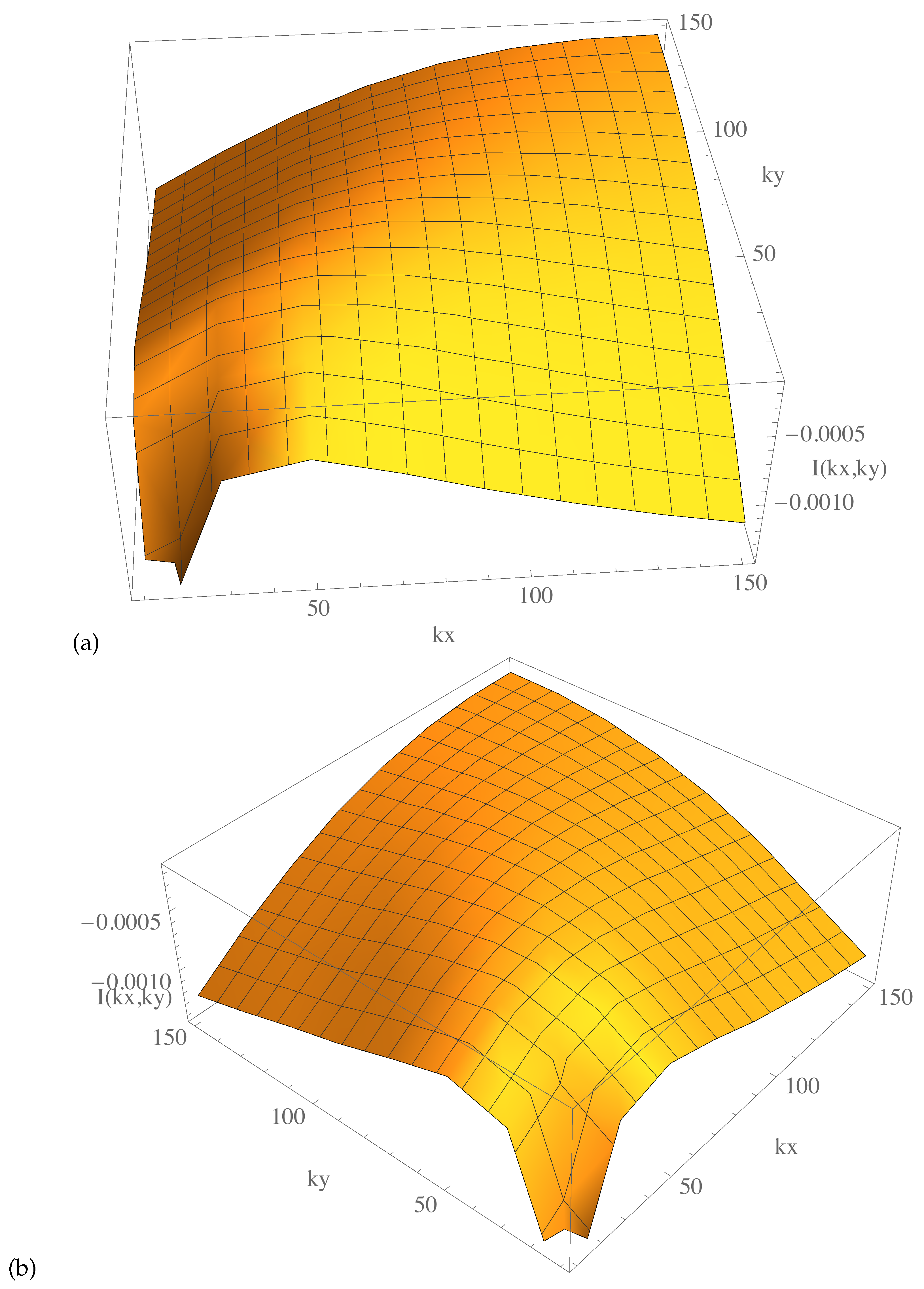
txy =
Table[NIntegrate[
I0bjacos[{kx, ky, kz}, {px, py, 0}], {px, 10, 150}, {py, 10, 150},
Method -> {"AdaptiveMonteCarlo", "MaxPoints" -> 100000},
WorkingPrecision -> MachinePrecision, MaxRecursion -> 100], {kx,
10, 150, 20}, {ky, 10, 150, 20}]
(*txy = Table[
NIntegrate[
I0bjacos[{kx, ky, kz}, {px, py, 0}], {px, 10, 150}, {py, 10, 150},
Method -> {"GlobalAdaptive", "MaxErrorIncreases" -> 3000},
WorkingPrecision -> MachinePrecision, MaxRecursion -> 30], {kx, 10,
150, 20}, {ky, 10, 150, 20}]*)
ListPlot3D[txy, PlotLegends -> Automatic,
AxesLabel -> {kx, ky, "I(kx,ky)"}, ClippingStyle -> None,
DataRange -> {{10, 150}, {10, 150}}]
References
- Kadomstev, B.B. Plasma turbulence, collection: Problems of Plasma Theory. Atomizdat 1964, 4. (In Russian) [Google Scholar]
- Galeev, A.A.; Karpman, V.I.; Sagdeev, R.Z. Multiparticle aspects of turbulent-plasma theory. Nuclear Fusion 1965, 5, 20. [Google Scholar] [CrossRef]
- Zakharov, V.E.; Filonenko, N.N. Weak turbulence of capillary waves. J. Appl. Mech. Tech. Phys. 1967, 8, 62–67. [Google Scholar] [CrossRef]
- Zakharov, V.E. Hamiltonian formalism for nonlinear waves. Physics-Uspekhi 1997, 40, 1087–1116. [Google Scholar] [CrossRef]
- Balk, A.M. On the Kolmogorov-Zakharov spectra of weak turbulence. Physica D 2000, 139, 137–157. [Google Scholar] [CrossRef]
- Choi, Y.; Lvov, Y.V.; Nazarenko, S. Wave Turbulence. Recent Res. Dev. Fluid Dyn. 2004, 5, 1–33. [Google Scholar]
- Nazarenko, S. Wave Turbulence; Springer: Berlin/Heidelberg, Germany, 2011. [Google Scholar]
- Galtier, S. Weak inertial-wave turbulence theory. Phys. Rev. E 2003, 68, 015301(R). [Google Scholar] [CrossRef] [PubMed]
- Galtier, S. Theory for helical turbulence under fast rotation. Phys. Rev. E 2014, 89, 041001. [Google Scholar] [CrossRef] [PubMed]
- Scott, J.F. Wave turbulence in a rotating channel. J. Fluid Mech. 2014, 741, 316–349. [Google Scholar] [CrossRef]
- Cambon, C.; Rubinstein, R.; Godeferd, F. Advances in wave turbulence: Rapidly rotating flows. New J. Phys. 2004, 6, 73. [Google Scholar] [CrossRef]
- Proudman, J. On the motion of solids in a liquid possessing vorticity. Proc. R. Soc. Lond. A 1916, 92, 408–424. [Google Scholar] [CrossRef]
- Taylor, G.I. Experiments on the motion of solid bodies in rotating fluids. Proc. R. Soc. Lond. A 1923, 104, 213–218. [Google Scholar] [CrossRef]
- Julien, K.; Knobloch, E.; Milliff, R.; Werne, J. Generalized quasi-geostrophy for spatially anistropic rotationally constrained flows. J. Fluid Mech. 2006, 555, 233–274. [Google Scholar] [CrossRef]
- Julien, K.; Knobloch, E. Reduced Models for Fluid Flows with Strong Constraints. J. Math. Phys. 2007, 48, 065405. [Google Scholar] [CrossRef]
- Embid, P.F.; Majda, A.J. Low Froude number limiting dynamics for stably stratified flow with small or finite Rossby numbers. Geophys. Astrophys. Fluid Dyn. 1998, 87, 1–30. [Google Scholar] [CrossRef]
- Thiele, M.; Muller, W. Structure and decay of rotating homogeneous turbulence. J. Fluid. Mech. 2009, 637, 425–442. [Google Scholar] [CrossRef]
- Morize, C.; Moisy, F. Energy decay of rotating turbulence with confinement effects. Phys. Fluids 2006, 18, 065107. [Google Scholar] [CrossRef]
- Smith, L.; Waleffe, F. Transfer of energy to two-dimensional large scales in forced, rotating three-dimensional turbulence. Phys. Fluids 1999, 11, 1608. [Google Scholar] [CrossRef]
- Bourouiba, L.; Bartello, P. The intermediate Rossby number range and two-dimensional-three-dimensional transfers in rotating decaying homogeneous turbulence. J. Fluid. Mech. 2007, 587, 139–161. [Google Scholar] [CrossRef]
- Mininni, P.D.; Pouquet, A. Rotating helical turbulence. I. Global evolution and spectral behavior. Phys. Fluids 2010, 22, 035105. [Google Scholar] [CrossRef]
- Teitelbaum, T.; Mininni, P.D. The decay of Batchelor and Saffman rotating turbulence. Phys. Rev. E 2012, 86, 066320. [Google Scholar] [CrossRef] [PubMed]
- Mininni, P.D.; Rosenberg, D.; Pouquet, A. Isotropization at small scales of rotating helically driven turbulence. J. Fluid Mech. 2012, 699, 263–269. [Google Scholar] [CrossRef]
- Pouquet, A.; Mininni, P.D. The interplay between helicity and rotation in turbulence: Implications for scaling laws and small-scale dynamics. Philos. Trans. R. Soc. A 2010, 368, 1635–1662. [Google Scholar] [CrossRef] [PubMed]
- Shepherd, T.G. Symmetries, conservation laws, and Hamiltonian structure in geophysical fluid dynamics. Adv. Geophys. 1990, 32, 287–339. [Google Scholar]
- Julien, K.; Knobloch, E.; Werne, J. A new class of equations for rotationally constrained flows. Theor. Comput. Fluid Dyn. 1998, 11, 251–261. [Google Scholar] [CrossRef]
- Nazarenko, S.; Scheckochihin, A. Critical balance in magnetohydrodynamics, rotating and stratified turbulence: Towards a universal scaling. J. Fluid Mech. 2011, 677, 134–153. [Google Scholar] [CrossRef]
- Greenspan, H.P. The Theory of Rotating Fluids; Cambridge University Press: Cambridge, UK, 1968. [Google Scholar]
- Lesieur, M. Décomposition d’un champ de vitesse non divergent en ondes d’hélicité. Observatoire de Nice Report, unpublished work. 1972. [Google Scholar]
- Zakharov, V.E.; L’vov, V.S.; Falkovich, G. Kolmogorov Spectra of Turbulence: Wave Turbulence; Springer: Berlin-Heidelberg, Germany, 1992. [Google Scholar]
- Hinch, E.J. Perturbation Methods; Cambridge University Press: Cambridge, UK, 1991. [Google Scholar]
- Bender, C.M.; Orzag, S.A. Advanced Mathematical Methods for Scientists And Engineers; Springer: New York, NY, USA, 1999. [Google Scholar]
- Kevorkian, J.; Cole, J. Perturbation Methods in Applied Mathematics; Springer: New York, NY, USA, 1996. [Google Scholar]
- Galtier, S.; Nazarenko, S.V.; Newell, A.C.; Pouquet, A. Anisotropic turbulence of Shear-Alfven waves. Astrophys. J. 2002, 564, L49–L52. [Google Scholar] [CrossRef]
- Abramov, R. A Simple Stochastic Parameterization for Reduced Models of Multiscale Dynamics. Fluids 2016, 1, 2. [Google Scholar] [CrossRef]
- Balk, A.M.; Nazarenko, S.V. Physical realizability of anisotropic weak turbulence Kolmogorov spectra. Zh. Eksp. Teor. Fiz. 1990, 97, 1827–1846. [Google Scholar]
- Lesieur, M. Turbulence in Fluids; Springer: Amsterdam, The Netherlands, 2008. [Google Scholar]
- Sen, A. A Tale of Waves and Eddies in a Sea of Rotating Turbulence. Ph.D. Dissertation, University of Colorado Boulder, Boulder, CO, USA, 2014. [Google Scholar]
- Newell, A.C.; Rumpf, B. Wave turbulence. Annu. Rev. Fluid Mech. 2011, 43, 59–78. [Google Scholar] [CrossRef]
- Kuznetsov, E.A. Turbulence of ion sound in a plasma located in a magnetic field. Zh. Eksp. Teor. Fiz. 1972, 62, 584–592. [Google Scholar]
- Orszag, S.A. Analytical theories of turbulence. J. Fluid Mech. 1970, 41, 363–386. [Google Scholar] [CrossRef]
- Orszag, S.A. Lectures on the Statistical Theory of Turbulence; Flow Research Incorporated: Wakefield, MA, USA, 1974. [Google Scholar]
- Pouquet, A.; Frisch, U.; Leorat, J. Strong MHD helical turbulence and the nonlinear dynamo effect. J. Fluid Mech. 1976, 77, 321–354. [Google Scholar] [CrossRef]
- Frederiksen, J.S.; O’Kane, T.J. Entropy, Closures and Subgrid Modeling. Entropy 2008, 10, 635–683. [Google Scholar] [CrossRef]
- Leith, C.E. Atmospheric Predictability and Two-Dimensional Turbulence. J. Atmos. Sci. 1971, 28, 145–161. [Google Scholar] [CrossRef]
- Bowman, J.C.; Krommes, J.A.; Ottaviani, M. The realizable Markovian closure. I. General theory, with application to three-wave dynamics. Phys. Fluids B 1993, 5, 3558–3589. [Google Scholar] [CrossRef]
- Bowman, J.C.; Krommes, J.A. The realizable Markovian closure and realizable test-field model. II. Application to anisotropic drift-wave dynamics. Phys. Plasmas 1997, 4, 3895–3909. [Google Scholar] [CrossRef]
- Krommes, J.A. Turbulence And Coherent Structures in Fluids, Plasmas and Nonlinear Medium; Shats, M., Punzmann, H., Eds.; World Scientific Publishing Co.: Singapore, 2006. [Google Scholar]
- Krommes, J.A. Mathematical and Physical Theory of Turbulence; Cannon, J., Shivamoggi, B., Eds.; Chapman and Hall/CRC: Boca Raton, FL, USA, 2006. [Google Scholar]
- Bowman, J.C. Rrealizable Markovian Statistical Closures: General Theory and Application to Drift-Wave Turbulence. Ph.D. Dissertation, Princeton University, Princeton, NJ, USA, 1992. [Google Scholar]
- LaCasce, J.H. Estimating Eulerian Energy Spectra from Drifters. Fluids 2016, 1, 33. [Google Scholar] [CrossRef]
- Connaughton, C. Numerical solutions of the isotropic 3-wave kinetic equation. Physica D 2009, 238, 2282–2297. [Google Scholar] [CrossRef]
- Bellet, F.; Godeferd, F.; Scott, J.; Cambon, C. Wave turbulence in rapidly rotating flows. J. Fluid. Mech. 2006, 562, 83–121. [Google Scholar] [CrossRef]
- Galtier, S.; Nazarenko, S.V.; Newell, A.C.; Pouquet, A. A weak turbulence theory for incompressible MHD. J. Plasma Phys. 2000, 63, 447–488. [Google Scholar] [CrossRef]
- Teitelbaum, T.; Mininni, P.D. Effect of Helicity and Rotation on the Free Decay of Turbulent Flows. Phys. Rev. Lett. 2009, 103, 014501. [Google Scholar] [CrossRef] [PubMed]
- Cardy, J.; Falkovich, G.; Gawedzki, K. Non-equilibrium Statistical Mechanics and Turbulence; Nazarenko, S., Zaboronski, O.V., Eds.; Cambridge University Press: Cambridge, UK, 2008. [Google Scholar]
- Janssen, P. Nonlinear four-wave interactions and freak waves. J. Phys. Oceanogr. 2003, 33.4. [Google Scholar] [CrossRef]
- Annenkov, S.; Shrira, V.I. Role of non-resonant interactions in the evolution of nonlinear random water wave fields. J. Fluid Mech. 2006, 561, 181–207. [Google Scholar] [CrossRef]
- Di Leoni, P.C.; Cobelli, P.J.; Mininni, P.D.; Dmitruk, P.; Matthaeus, W.H. Quantification of the strength of inertial waves in a rotating turbulent flow. arXiv, 2013; arXiv:1310.4214. [Google Scholar]
- Kartashova, E. Nonlinear Resonance Analysis; Cambridge Uuniversity Press: Cambridge, UK, 2010. [Google Scholar]
- Berloff, P. Dynamically Consistent Parameterization of Mesoscale Eddies—Part II: Eddy Fluxes and Diffusivity from Transient Impulses. Fluids 2016, 1, 22. [Google Scholar] [CrossRef]


© 2017 by the author. Licensee MDPI, Basel, Switzerland. This article is an open access article distributed under the terms and conditions of the Creative Commons Attribution (CC BY) license (http://creativecommons.org/licenses/by/4.0/).
Share and Cite
Sen, A. Anisotropic Wave Turbulence for Reduced Hydrodynamics with Rotationally Constrained Slow Inertial Waves. Fluids 2017, 2, 28. https://doi.org/10.3390/fluids2020028
Sen A. Anisotropic Wave Turbulence for Reduced Hydrodynamics with Rotationally Constrained Slow Inertial Waves. Fluids. 2017; 2(2):28. https://doi.org/10.3390/fluids2020028
Chicago/Turabian StyleSen, Amrik. 2017. "Anisotropic Wave Turbulence for Reduced Hydrodynamics with Rotationally Constrained Slow Inertial Waves" Fluids 2, no. 2: 28. https://doi.org/10.3390/fluids2020028
APA StyleSen, A. (2017). Anisotropic Wave Turbulence for Reduced Hydrodynamics with Rotationally Constrained Slow Inertial Waves. Fluids, 2(2), 28. https://doi.org/10.3390/fluids2020028