Numerical Study of a 3D Eulerian Monolithic Formulation for Incompressible Fluid-Structures Systems

Abstract
:1. Introduction
- The fully Eulerian formulation is derived in Section 1.
- In Section 2 the equations are discretized implicitly in time as in [18,19]; then the displacements are eliminated and a non-linear system for the velocities and pressures remains. Spatial discretization is obtained by using stable finite element spaces like linear pressures and quadratic velocities on a tetrahedral mesh.
- In Section 3 it is shown that the energy decays at each time step, which is an indication that the method is robust.
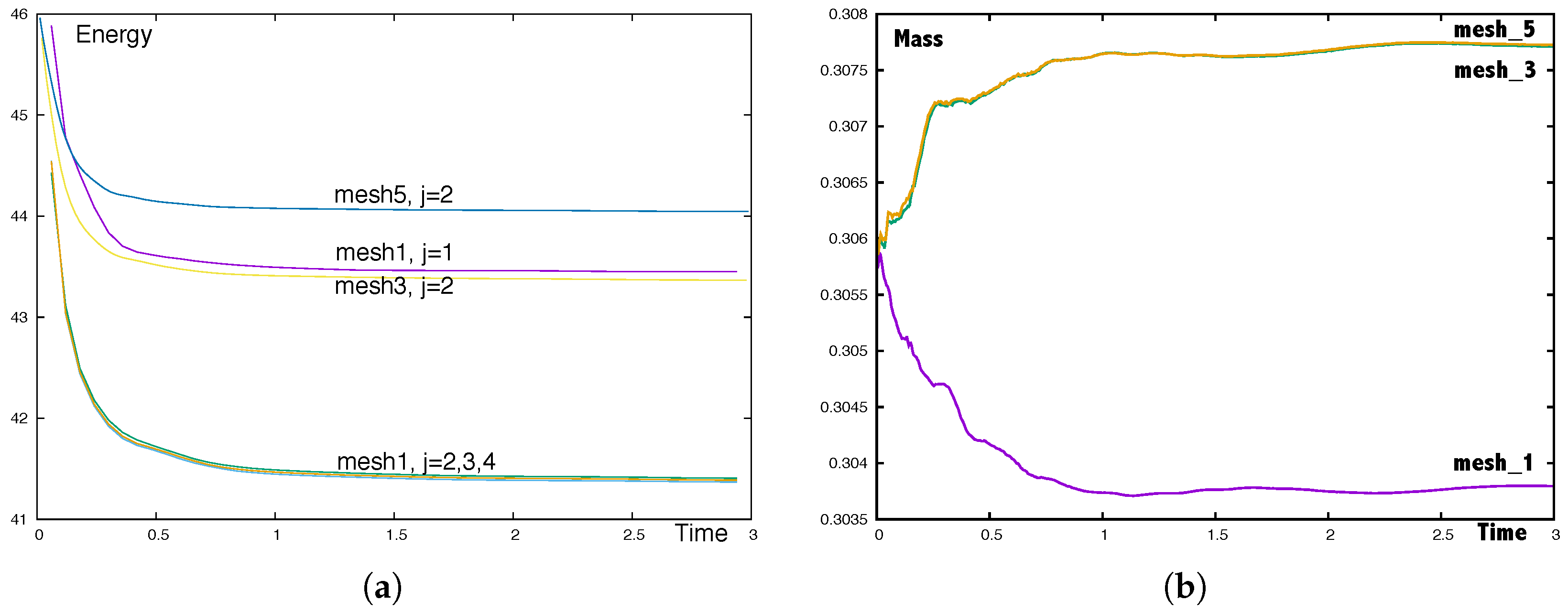
- Finally, in Section 4, the method is implemented in 2D for axisymmetric systems and in 3D for general systems. Energy decrease, mass conservation and convergence are analyzed on an axisymmetric case: an elastic torus in a cylindrical canister filled with a fluid at a Reynolds number of a few hundred. Then, the method is carefully evaluated on the test case proposed in [20] and comparisons with previous publications are made.
2. Derivation of the Formulation from the General Laws of Continuum Mechanics
2.1. Notations
- be the fluid–structure interface, and be the boundary of ,
- be the part of where the structure is clamped or the fluid does not slip. It is assumed to be independent of t.
- is the Lagrangian position at t of ,
- is the displacement,
- is the Eulerian velocity of the deformation at t and ,
- is the transposed gradient of the deformation,
- is the Jacobian of the deformation.
- , the density,
- , the stress tensor.
2.2. Conservation Laws
2.3. Constitutive Equations
- For a Newtonian incompressible fluid,
- For an hyperelastic incompressible material,
2.4. The Mooney–Rivlin 3D Stress Tensor
2.5. From 3D to 2D
2.6. Variational Formulation
3. Numerical Schemes
3.1. Characteristic-Galerkin Derivatives
3.2. A Monolithic Time–Discrete Variational Formulation
- One may wonder why the scheme is applied to and not to . Note that is convected by the velocity . Hence . This shows that discretizing the total derivative of or the total derivative of gives the same scheme:
3.3. Spacial Discretization with Finite Elements
3.4. Solution Algorithm
- Set , , , , ,
- Solve system (21). In this study a direct solver is used for the linear system.
- Set , , ; update and .
- If not converged return to step 2.
4. Stability of the Scheme
4.1. Conservation of Energy
4.2. Stability of the Scheme Discretized in Time
4.3. Energy Inequality for the Fully Discrete Scheme
5. Numerical Tests
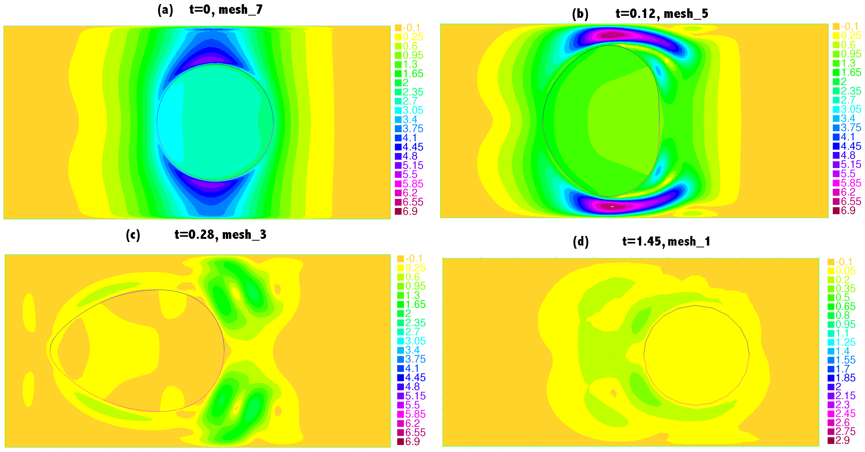
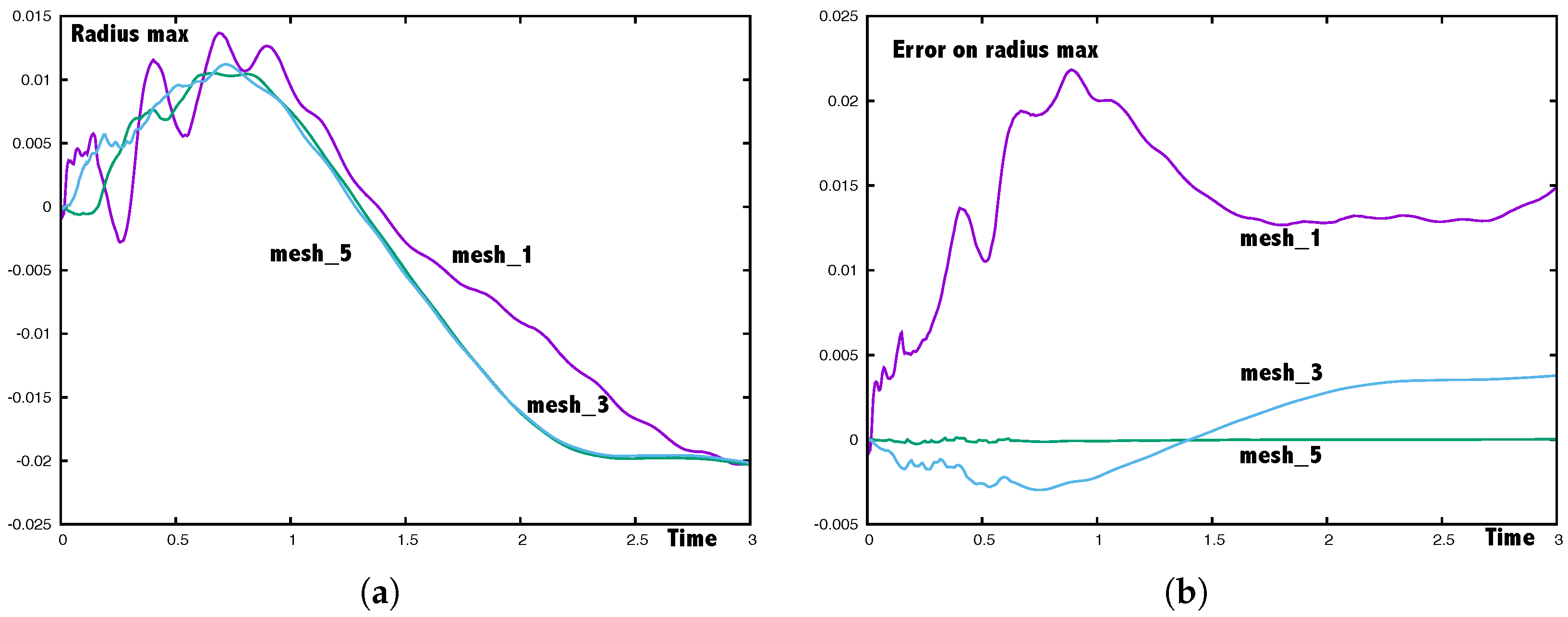
5.1. An Axisymmetric Torus
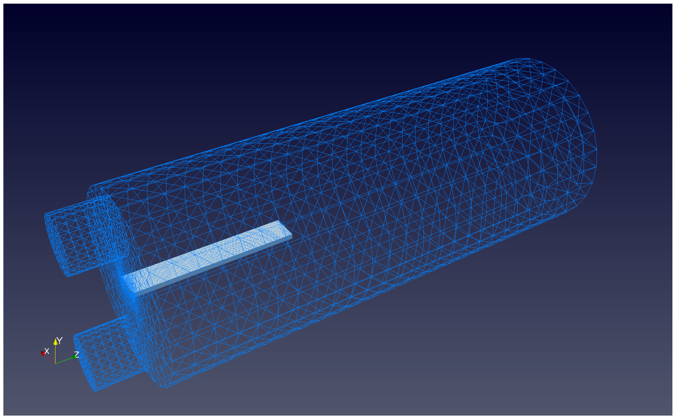
5.2. Clamped Structure in a Fluid
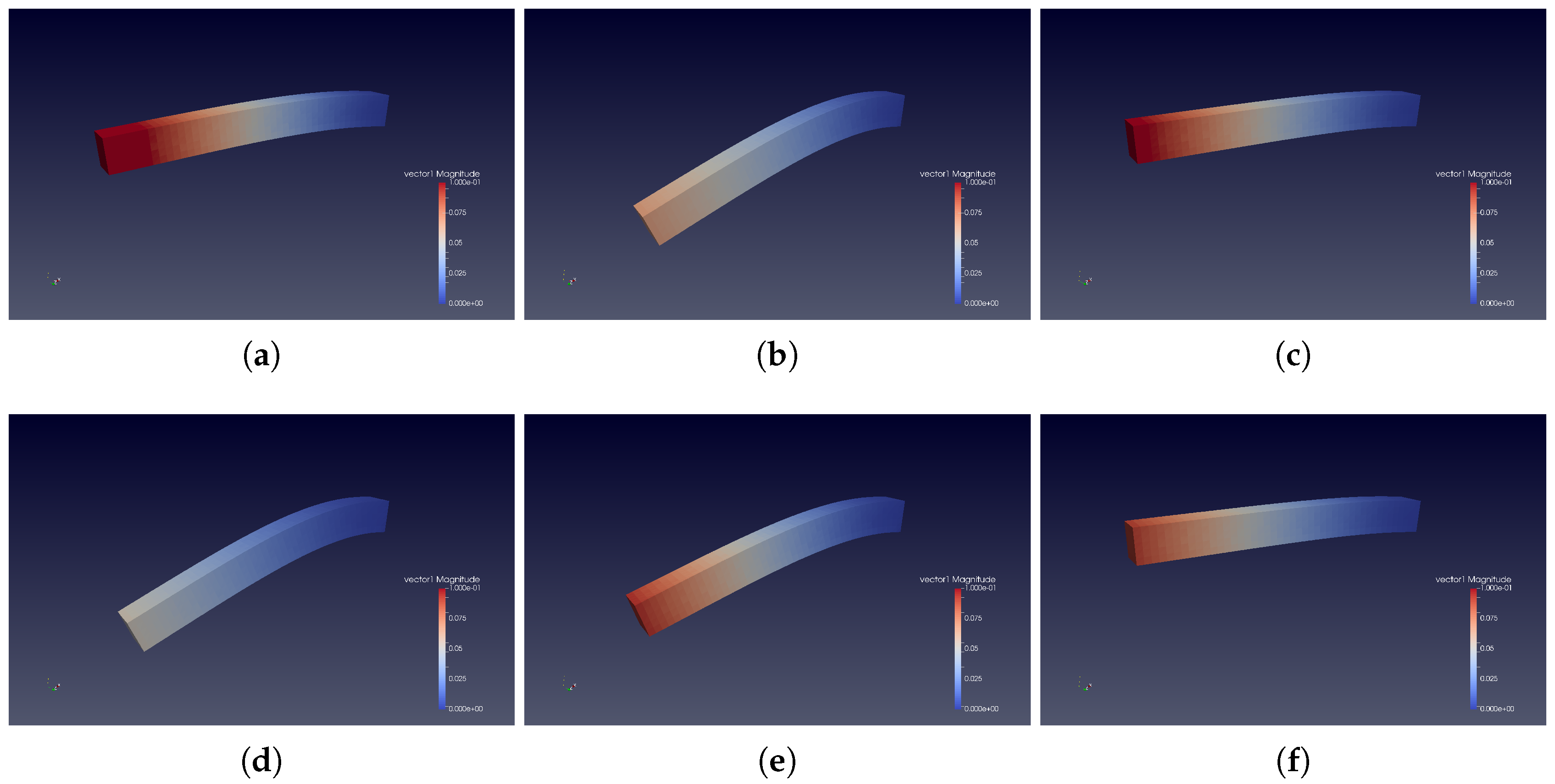
5.2.1. Free-Fall of a Clamped Structure in Vacuum
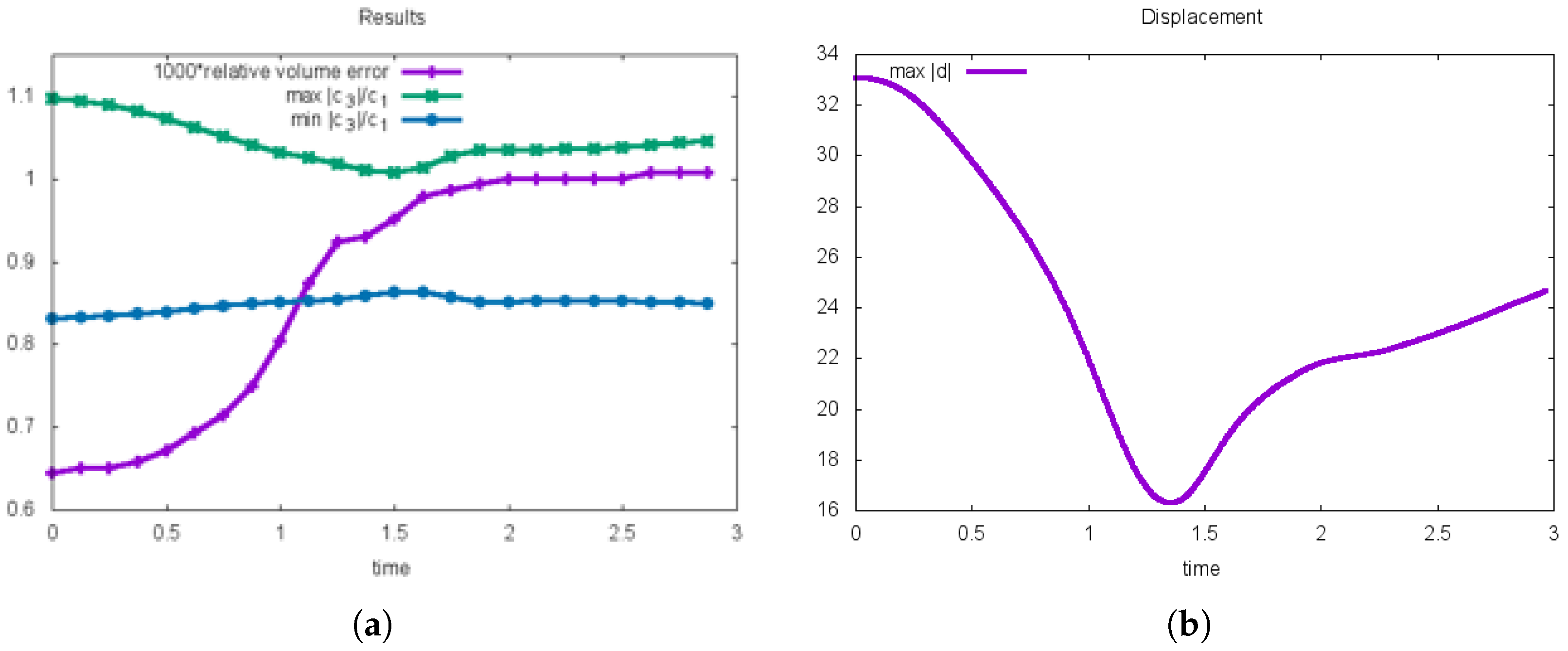
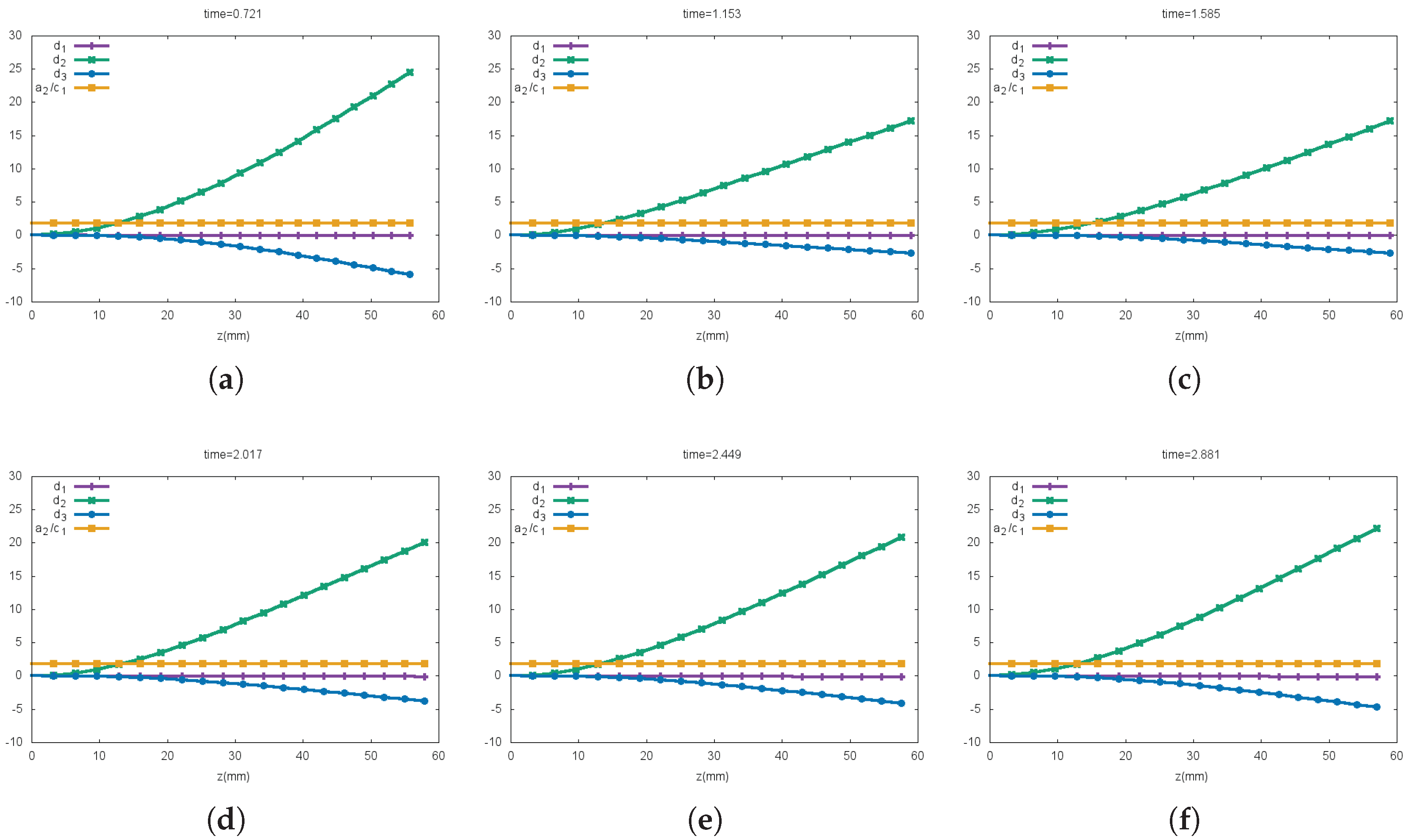
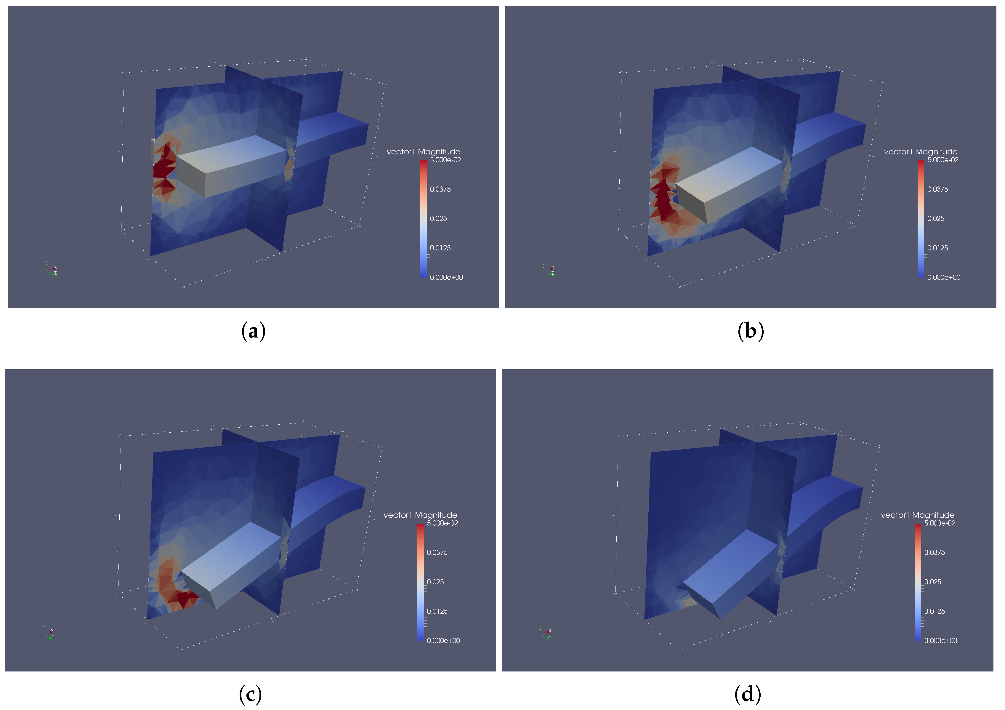
5.2.2. Free-Fall of a Clamped Beam in a Fluid
5.3. The Benchmark
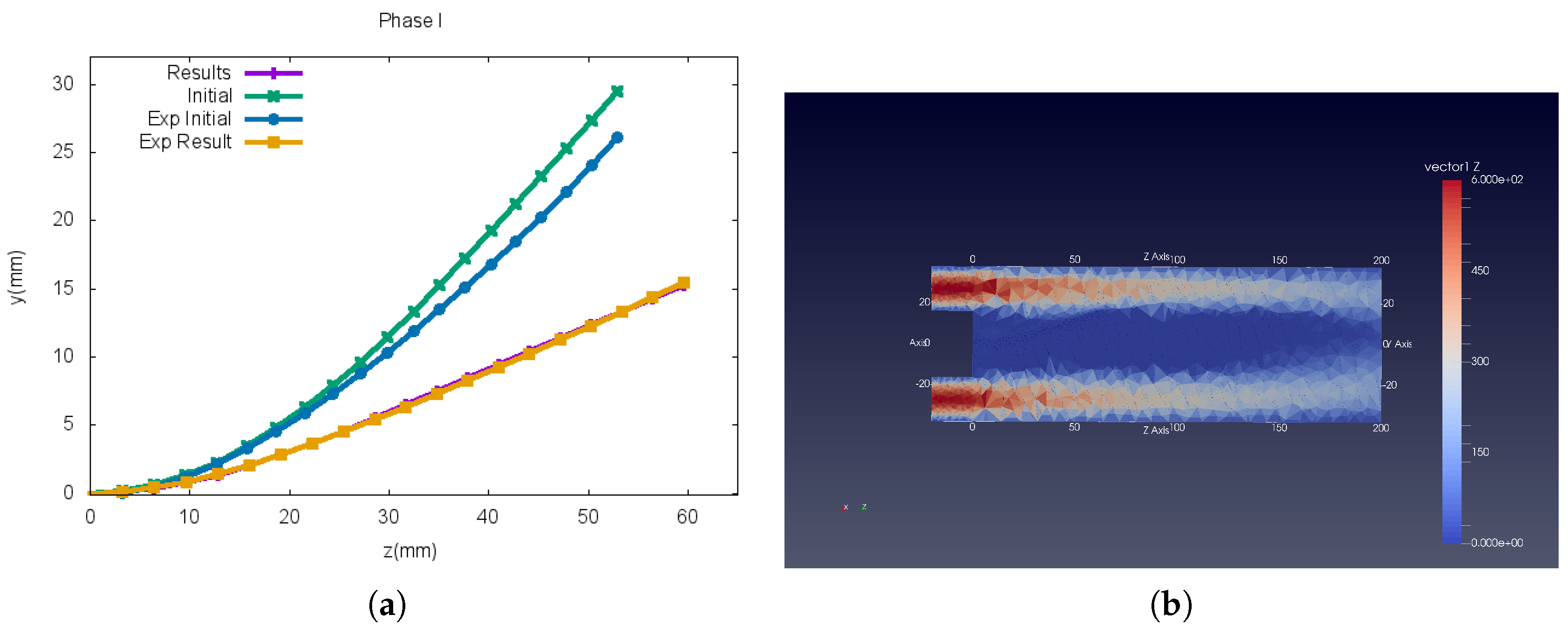
5.3.1. Phase I
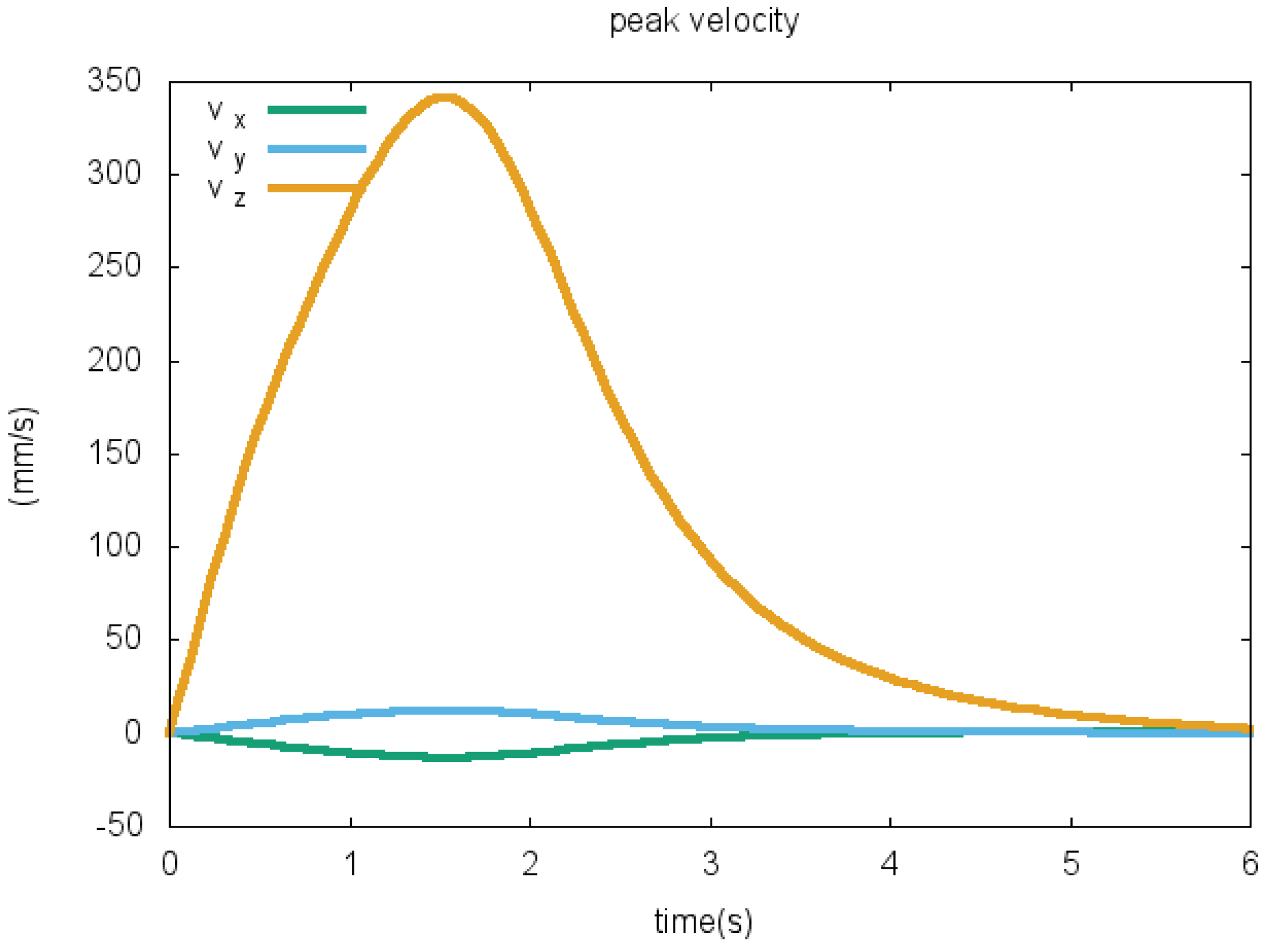
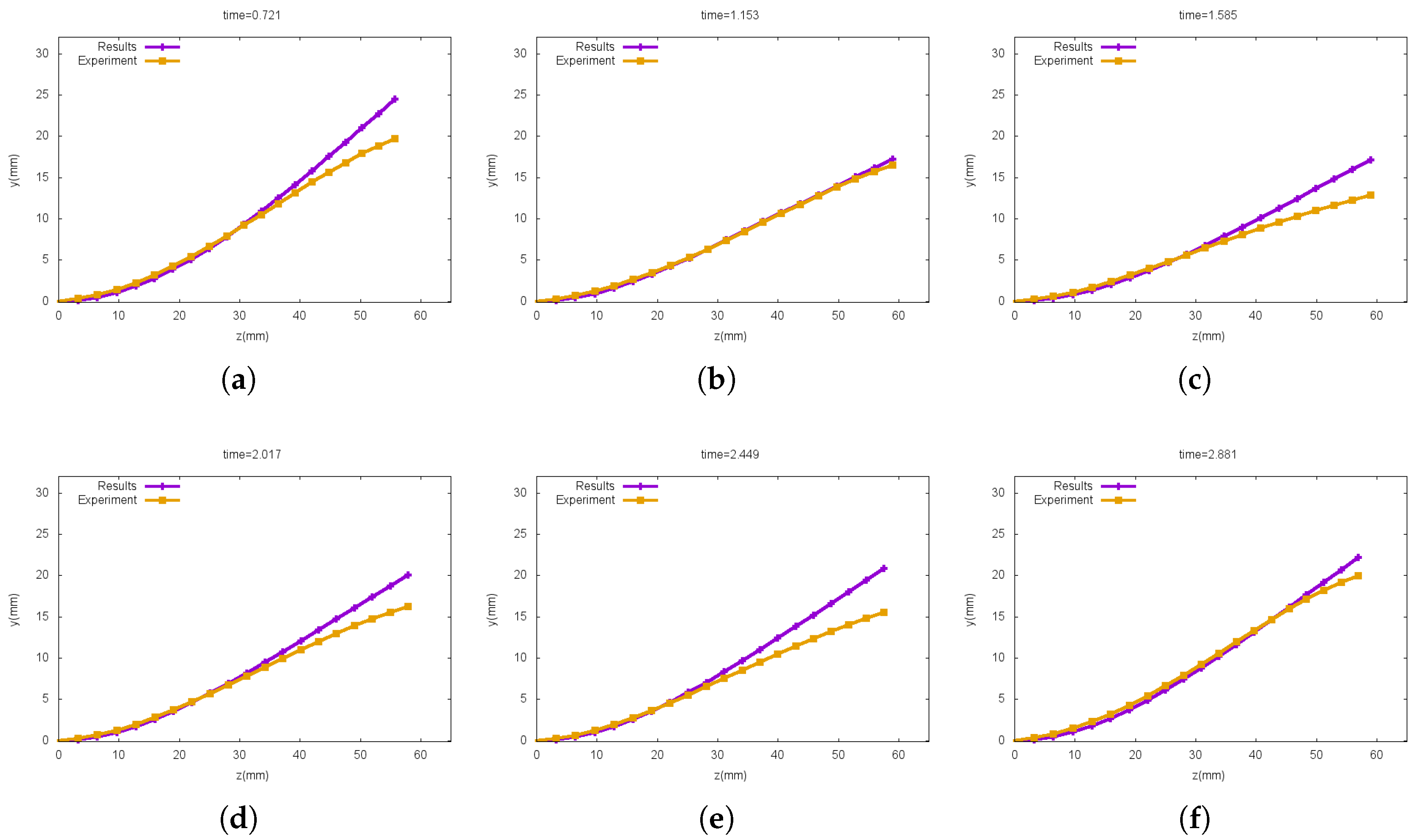
5.3.2. Phase II
5.3.3. Variation of Coefficient
6. Conclusions
Acknowledgments
Author Contributions
Conflicts of Interest
References
- Martins, J. Wing design via numerical optimization. SIAG OPT Views News 2015, 23, 2–7. [Google Scholar]
- Peskin, C.S. The immersed boundary method. Acta Numer. 2002, 11, 479–517. [Google Scholar] [CrossRef]
- Formaggia, L.; Quarteroni, A.; Veneziani, A. (Eds.) Cardiovascular Mathematics; Springer: Milano, Italy, 2009. [Google Scholar]
- Hauret, P. Numerical Methods for the Dynamic Analysis of Two-Scale Incompressible Nonlinear Structures. Ph.D. Thesis, Ecole Polytechnique, Paris, France, 2004. [Google Scholar]
- Hron, J.; Turek, S. A monolithic FEM solver for an ALE formulation of fluid-structure interaction with configuration for numerical benchmarking. In Proceedings of the European Conference on Computational Fluid Dynamics, Egmond aan Zee, The Netherlands, 5–8 September 2006. [Google Scholar]
- Basting, S.; Quaini, A.; Čanić, S.; Glowinski, R. Extended ALE Method for fluid-structure interaction problems with large structural displacements. J. Comput. Phys. 2017, 331, 312–336. [Google Scholar] [CrossRef]
- Liu, J. A second-order changing-connectivity ALE scheme and its application to FSI with large convection of fluids and near contact of structures. J. Comput. Phys. 2016, 304, 380–423. [Google Scholar] [CrossRef]
- Boffi, D.; Cavallini, N.; Gastaldi, L. The finite element immersed boundary method with distributed lagrange multiplier. SIAM J. Numer. Anal. 2015, 53, 2584–2604. [Google Scholar] [CrossRef]
- Wang, Y.; Jimack, P.K.; Walkley, M.A. A one-field monolithic fictitious domain method for fluid-structure interactions. Comput. Methods Appl. Mech. Eng. 2017, 317, 1146–1168. [Google Scholar] [CrossRef]
- Maury, B.; Glowinski, R. Fluid-particle flow: A symmetric formulation. C. R. Acad. Sci. Ser. I Math. 1997, 324, 1079–1084. [Google Scholar] [CrossRef]
- Glowinski, R.; Pan, T.W.; Hesla, T.I.; Joseph, D.D.; Périaux, J. A fictitious domain approach to the direct numerical simulation of incompressible viscous flow past moving rigid bodies: Application to particulate flow. J. Comput. Phys. 2001, 169, 363–426. [Google Scholar] [CrossRef]
- Liu, C.; Walkington, N.J. An eulerian description of fluids containing visco-elastic particles. Arch. Ration. Mech. Anal. 2001, 159, 229–252. [Google Scholar] [CrossRef]
- Rannacher, R.; Richter, T. An Adaptive Finite Element Method for Fluid-Structure Interaction Problems Based on a Fully Eulerian Formulation. In Fluid Structure Interaction II; Springer: Berlin/Heidelberg, Germany, 2011; pp. 159–191. [Google Scholar]
- Dunne, T.; Rannacher, R. Adaptive Finite Element Approximation of Fluid-Structure Interaction Based on an Eulerian Variational Formulation. In Fluid-Structure Interaction; Springer: Berlin/Heidelberg, Germany, 2006; pp. 110–145. [Google Scholar]
- Richter, T. A Fully Eulerian formulation for fluid-structure-interaction problems. J. Comput. Phys. 2013, 233, 227–240. [Google Scholar] [CrossRef]
- Wick, T. Fully Eulerian fluid-structure interaction for time-dependent problems. Comput. Methods Appl. Mech. Eng. 2013, 255, 14–26. [Google Scholar] [CrossRef]
- Pironneau, O. Numerical Study of a Monolithic Fluid-Structure Formulation. In Variational Analysis and Aerospace Engineering; Mohammadi, B., Frediani, A., Cipolla, V., Eds.; Number 116 in Springer Optimization and Its Applications; Springer International Publishing: Cham, Switzerland, 2016; pp. 401–420. [Google Scholar]
- Hecht, F.; Pironneau, O. An energy stable monolithic eulerian fluid-structure finite element method. Int. J. Numer. Methods Fluid 2017. [Google Scholar] [CrossRef]
- Pironneau, O. An energy preserving monolithic eulerian fluid-structure numerical scheme. arXiv 2016. [Google Scholar]
- Hessenthaler, A.; Gaddum, N.R.; Holub, O.; Sinkus, R.; Röhrle, O.; Nordsletten, D.A. Experiment for validation of fluid-structure interaction models and algorithms. Int. J. Numer. Methods Biomed. Eng. 2016. [Google Scholar] [CrossRef] [PubMed]
- Pironneau, O. On the transport-diffusion algorithm and its applications to the Navier-Stokes equations. Numer. Math. 1982, 38, 309–332. [Google Scholar] [CrossRef]
- Boulakia, M. Existence of weak solutions for the motion of an elastic structure in an incompressible viscous fluid. C. R. Math. 2003, 336, 985–990. [Google Scholar] [CrossRef]
- Coutand, D.; Shkoller, S. Motion of an Elastic Solid inside an Incompressible Viscous Fluid. Arch. Ration. Mech. Anal. 2005, 176, 25–102. [Google Scholar] [CrossRef]
- Raymond, J.P.; Vanninathan, M. A fluid-structure model coupling the Navier-Stokes equations and the Lamé system. J. Math. Pures Appl. 2014, 3, 546–596. [Google Scholar] [CrossRef]
- Hecht, F. New development in freefem++. J. Numer. Math. 2013, 20, 251–266. [Google Scholar] [CrossRef]
- Larma, M.L. Coupling Schemes and Unfitted Mesh Methods for Fluid-Structure Interaction. Ph.D. Thesis, Université Pierre et Marie Curie (Paris VI), Paris, France, 2016. [Google Scholar]


| 7.73 | 1.38 | 0.24 | 3.59 | 1 | |||||
| 14.95 | 11.88 | 2.06 | 4.95 | 1 | |||||
| 367.10 | 363.40 | 1.21 | 3.76 | 1 |
© 2017 by the authors. Licensee MDPI, Basel, Switzerland. This article is an open access article distributed under the terms and conditions of the Creative Commons Attribution (CC BY) license (http://creativecommons.org/licenses/by/4.0/).
Share and Cite
Chiang, C.-Y.; Pironneau, O.; Sheu, T.W.H.; Thiriet, M. Numerical Study of a 3D Eulerian Monolithic Formulation for Incompressible Fluid-Structures Systems. Fluids 2017, 2, 34. https://doi.org/10.3390/fluids2020034
Chiang C-Y, Pironneau O, Sheu TWH, Thiriet M. Numerical Study of a 3D Eulerian Monolithic Formulation for Incompressible Fluid-Structures Systems. Fluids. 2017; 2(2):34. https://doi.org/10.3390/fluids2020034
Chicago/Turabian StyleChiang, Chen-Yu, Olivier Pironneau, Tony W. H. Sheu, and Marc Thiriet. 2017. "Numerical Study of a 3D Eulerian Monolithic Formulation for Incompressible Fluid-Structures Systems" Fluids 2, no. 2: 34. https://doi.org/10.3390/fluids2020034
APA StyleChiang, C.-Y., Pironneau, O., Sheu, T. W. H., & Thiriet, M. (2017). Numerical Study of a 3D Eulerian Monolithic Formulation for Incompressible Fluid-Structures Systems. Fluids, 2(2), 34. https://doi.org/10.3390/fluids2020034