Article

In Vitro Study of the Effect of an Abdominal Aortic Aneurysm on Pulse Wave Velocity Measurement Using 4D-Flow MRI

1
Instituto de Medicina Traslacional, Trasplante y Bioingeniería (IMETTyB), Universidad Favaloro—CONICET, Buenos Aires C1078AAI, Argentina
2
Instituto de Investigación en Tecnologías y Ciencias de la Ingeniería, Universidad Nacional del Comahue-CONICET, Neuquén Q8300IBX, Argentina
3
Centro Universitario de Imágenes Médicas, Escuela de Ciencia y Tecnología, Universidad Nacional de San Martín, Buenos Aires B1650, Argentina
4
Instituto de Industria, Universidad Nacional de General Sarmiento, Los Polvorines B1613GSX, Argentina
*
Author to whom correspondence should be addressed.
Fluids 2026, 11(7), 177; https://doi.org/10.3390/fluids11070177
Submission received: 1 June 2026 / Revised: 3 July 2026 / Accepted: 9 July 2026 / Published: 13 July 2026
(This article belongs to the Special Issue Recent Advances in Cardiovascular Flows, 2nd Edition)

Abstract

Abdominal aortic aneurysm (AAA) is a critical condition with high rupture risk, and the maximum diameter alone is insufficient for prediction. Pulse wave velocity (PWV), a surrogate of aortic stiffness, can be estimated using 4D-Flow magnetic resonance imaging (MRI), but requires validation under dilated conditions. This in vitro study examined the relationship between PWV and stiffness by comparing healthy and aneurysmal compliant aortic models. Two latex phantoms were fabricated to represent normal and AAA geometries. A circulatory MRI-compatible system simulated physiological inlet flow, with flow rates measured across perpendicular planes using 4D- and 2D-Flow MRI. PWV was derived from transit times of the systolic upstroke and interplane distances. Complementary 1D numerical simulations and laboratory flowmeter measurements were performed. Although the wall elasticity and thickness were identical, PWV in the healthy model ranged from 6.2 to 7.7 m/s and in the aneurysmal model it ranged from 14.2 to 15 m/s. This increase was confirmed by temporal overlap of thoracic flow curves and reduced slope in the transit time–distance regression. Results were consistent across simulations, 2D-Flow, and flowmeter data. Findings highlight that indirect 4D-Flow assessment of thoracic stiffness in the presence of AAA must account for wave reflections introduced by dilation, which significantly alter PWV estimation.

1. Introduction

An abdominal aortic aneurysm (AAA) is a pathological dilation of the arterial wall. The size and growth of an AAA are associated with an increased risk of rupture [1]. Patients diagnosed with aortic diseases require regular clinical follow-up and assessment of anatomical progression. This is typically estimated using echocardiography, computed tomography or magnetic resonance imaging (MRI) [2]. When making therapeutic decisions, the quantification of the maximum diameter and other anatomical features plays a predominant role, whereas functional biomechanical analyses, such as estimates of arterial stiffness, are less common [3]. This is likely due to the complex flow pattern caused by dilation and its impact on the calculation of stiffness biomarkers [4]. Using advanced MRI techniques to determine arterial wall stiffness in the dilated region is likely to complement anatomical measurements and reduce uncertainty in predicting the risk of rupture.
Pulse wave velocity (PWV) is a widely used biomarker of aortic stiffness. It is sensitive to aging and can predict cardiovascular events [5]. There are numerous techniques and devices for quantifying PWV non-invasively, with the carotid–femoral measurement being the most widely used [6]. This propagation velocity is generally estimated as the ratio of the distance between two pressure (or flow) measurement points to the transit time (TT) between the signals. Recently, 4D-Flow MRI has been used to estimate aortic PWV as it enables the precise measurement of both the TT between two aortic flow curves and the distance between them [7]. However, estimating PWV is challenging in the presence of aortic dilation that produces complex flow patterns and reflected waves [8]. In this context, an in vitro study in a controlled environment that is compatible with routine 4D-Flow acquisitions can help to investigate whether the association between PWV and arterial stiffness remains valid in the presence of AAA.
Aortic PWV increases with arterial stiffness, but it is an indirect indicator. In other words, while it is positively associated with arterial wall elasticity, it also depends on other relevant factors. One way to clarify the relationship between PWV and arterial stiffness is to use simplified models. Perhaps the best-known of these models is described by the Moens–Korteweg (M-K) equation, which assumes idealized conditions in which the artery is a uniform tube of homogeneous elasticity and infinite length to ensure the absence of reflected waves [9]. According to the M-K equation, PWV increases proportionally to the square root of the incremental elastic modulus of the arterial wall (Einc) and its thickness (h), and inversely to blood density (ρ) and diameter (D) ( P W V M K 2 = Einc.h/(ρ.D)). Therefore, in the presence of arterial dilation, the model predicts a decrease in PWV if elasticity and wall thickness remain unchanged. Conversely, the stiffening of an aneurysmal sac would produce a modest increase in PWV, which would be counterbalanced by dilation [10].
A recent systematic review examined 68 in vitro studies investigating thoracic or abdominal aortic aneurysms, 47 of which focused on arterial biomechanics in closed circulatory systems [11]. Various laboratory instruments are available to generate physiological aortic pressure and flow waves in compliant models [12,13]; however, only a few are compatible with 4D-Flow MRI acquisitions to quantify aortic biomechanics [14]. In vitro studies using 4D-Flow have validated the estimation of stiffness in short, uniform, compliant arterial models using different PWV estimations [15]. The variety of methods for estimating PWV using 4D-Flow has also been studied in patients [16]. A recent in vitro 4D-Flow study on compliant aortic models made of silicone with varying stiffness demonstrates the potential of using PWV to estimate stiffness in healthy geometries, while also identifying the main limitations associated with wave reflection [17]. Distinct wave reflections are produced by changes in arterial geometry and elastic mismatch, which directly impact PWV assessment. Stenosis and aneurysms have been studied in depth in vitro, albeit using laboratory equipment on long tubes [18]. These studies reveal how reflections impact flow signals: a stenosis produces a retrograde reflected flow wave that decreases peak flow in proximal regions, whereas a dilation produces an anterograde suction effect that increases maximum flow in the segment proximal to the aneurysm. To the best of our knowledge, there are no reports of similar studies on AAA using 4D-Flow MRI in aortic models with more realistic shapes and lengths.
This in vitro study aimed to investigate the association between PWV and arterial stiffness in a controlled environment using 4D-Flow MRI by comparing latex aortic models with and without AAA, which had constant elasticity and wall thickness. Specifically, the study analyzed the impact of reflections caused by the AAA on flow curves and how this affects PWV estimation. This study investigates the hypothesis that dilation produces reflections that significantly affect the ability of PWV to describe regional aortic stiffness.

2. Materials and Methods

2.1. Compliant Aorta Models

Three-dimensional (3D) models of a healthy and a diseased aorta were created using numerical data on an average aortic shape derived from 500 healthy subjects provided in a previous study [19]. Model #1 represented a healthy aorta and in model #2 the abdominal portion was manually edited to add an aneurysm with an ellipsoid form (Figure 1). Model #1 for the healthy aorta had the following dimensions: 400 mm long, 20 mm in diameter and a wall thickness of 0.94 mm. Model #2 with the abdominal aneurysm was 400 mm long, with a diameter of 20 mm, and a wall thickness of 0.94 mm. The ellipsoidal abdominal aneurysm was 60 mm long and had a maximum diameter of 45 mm, with its centroid located 165 mm vertically below the center of the aortic arch and 290 mm from the inlet along the centerline. For both models, proper meshes of the aortic lumen were manually generated using Slic3r (slic3r.org, v. 1.3) and Autodesk Meshmixer (meshmixer.com, v. 3.5). The models retained part of the morphology of the thoracic and abdominal aorta, but tapering, aortic arc arteries and bifurcations were removed. The two 3D models were materialized using a 3D printer and used as molds to fabricate two latex aortas. Details of the fabrication can be found in a previous article [20]. The elasticity of the latex was assessed through uniaxial tensile tests (Tinius Olsen testing machine, model H5K-W, Horsham, PA, USA) and resulted in E ≈ 990.1 kPa.

2.2. Flow Circuit Setup

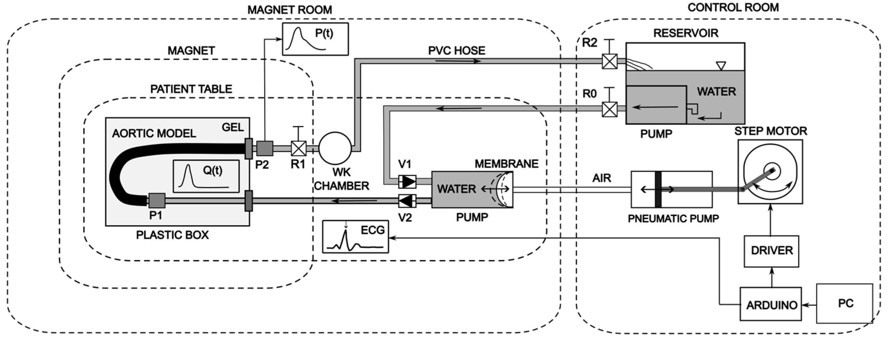
The flow simulator consisted of a recently developed closed circuit compatible with MRI (Figure 2) [20]. Briefly, an Arduino Due system controlled the pumping and also generated a synthetic electrocardiogram signal required for MRI synchronization. The heart rate was set at 60 bpm (cardiac cycle of 1000 ms). The resonator’s control room contained all the equipment that was either incompatible with the MRI magnet or able to act as a source of radiofrequency noise. This equipment included a 20 L liquid reservoir, a pneumatic piston moved by a stepper motor and a crank for providing the pulsatile motion, as explained below. The average inflow and outflow rates of the reservoir were controlled for pressure and flow adjustment by three shut-off valves (R0, R1 and R2). The remaining components, consisting of a non-ferromagnetic pneumatic pump with an elastic diaphragm for fluid motion modulation, two unidirectional valves, and the aortic model, were positioned inside the magnet room on the exam table and connected via plastic hoses. A first hose enters the pneumatic pump to regulate the displacement of the silicone diaphragm in contact with the liquid. A second hose, containing liquid from the fluid reservoir, enters the diaphragm pump through a first unidirectional valve (V1). The elastic diaphragm modulates the pulsatile liquid, which then exits the pump through another hose and passes through a second unidirectional valve (V2) before finally entering the aortic model. The compliant aorta models were encased in a plastic box and embedded in ultrasound gel. The aortic models were placed approximately 6 m away from the fluid reservoir. The Faraday cage passage serves as the connecting passage for the three hoses, one for air and two for fluid supply and return.

2.3. Imaging Experiments

Imaging experiments were performed using a 3T MRI scanner (MAGNETOM Prisma, Siemens Healthineers, Erlangen, Germany). A total of 12 L of water mixed with 2.5 mL of contrast agent solution (376.9 mg/mL meglumine gadoterate) were used in the experiment. The box containing the aortic model was covered with an 18-channel chest coil. Before each scan, pressure at the aortic outlet was measured using a disposable blood pressure transducer (PT111103, Acemedical, Seoul, Republic of Korea) and a multiparameter monitor (Advisor 9200 Vital Signs Monitor, BCI, Waukesha, WI, USA). The protocol steps were as follows: (i) all the components of the phantom were set up without liquid on the exam table and in the control room, (ii) the air and liquid hoses were connected, (iii) all fluid lines were filled with liquid, the steady flow pump located inside the reservoir was turned on and bubbles were removed, (iv) the pulsatile pump was energized, pressures were adjusted and recorded, and the monitor was disconnected, (v) 2D- and 4D-Flow acquisitions were performed.
A retrospective 2D-Flow acquisition orthogonal to the aortic lumen cross-section was performed at 10 planes along the compliant model #1 and at 13 planes for model #2. The parameters for the acquisition were encoding velocity (venc) = 120 cm/s, in-plane pixel size = 0.75 mm × 0.75 mm, slice thickness = 6 mm, field of view = 85 mm × 144 mm, TE = 3.5 ms, TR = 48 ms, flip angle = 20° and number of temporal frames = 50 (20 ms time resolution).
A prospective 4D-Flow acquisition supplied by the manufacturer was employed (fl3d1r code). It was performed with Cartesian k-space sampling, venc = 120 cm/s, pixel size of 2 mm in all three dimensions, FOV = 87 × 315 × 224 mm, TE = 3 ms, TR = 22 ms, flip angle = 7° and 40 reconstructed cardiac phases (25 ms of effective temporal resolution). The image data was corrected for Maxwell term during reconstruction and background phase offset correction for eddy currents was applied during post-processing using a third-order fitting of the static region [21]. Each 4D-Flow acquisition lasted approximately 40 min. The two aortas were studied on the same day, one after the other, using the same configurations.

2.4. Image Analysis for Flow Rate Measurements

All image processing was performed using a custom computer platform (www.lattido.com, Buenos Aires, Argentina) programmed with C# in our biomedical engineering lab as described elsewhere [10,22]. Briefly, this platform allows the user to visualize the 2D- and 4D-Flow acquisitions in standard panels, to superimpose magnitude intensities with colored velocities, to estimate streamlines and to interactively draw regions of interest (ROIs) around the aortic cross-sectional area to estimate flow rates and volumes as explained before [20]. Details of the numeric method to estimate flow through the ROIs are presented in Appendix A.

2.5. Computational 1D Model Simulation

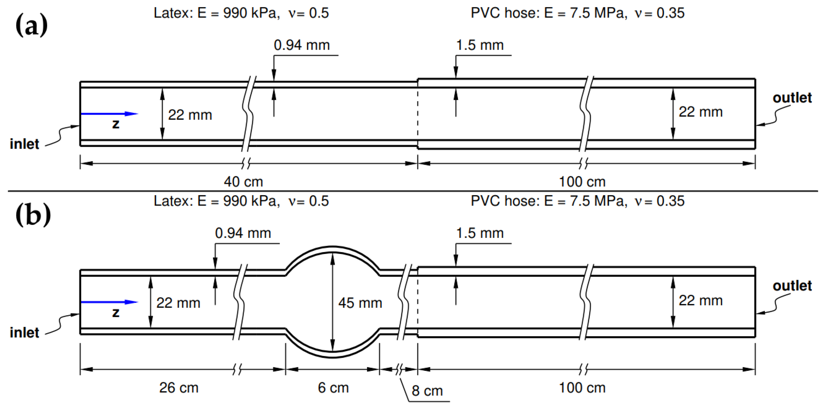
A one-dimensional (1D) computational model was calculated at a reduced computational cost to emulate the main wave reflections observed in the flow circuit setup for the two aortic models. It was assumed that the flow was incompressible and isothermal, and that the elasticity of the aortic wall was linear. Under these assumptions, the governing equations for fluid flow were the 1D continuity and momentum conservation equations [23,24], complemented by the relationship between aortic pressure and cross-sectional area proposed by Absi [25]. These governing equations were solved using the method of characteristics [26]. The solution advanced explicitly in time with a maximum time step bounded by the stability condition CFL < 1, where CFL is the Courant–Friedrichs–Lewy number. The domain consisted of two coupled cylinders of 40 cm and 100 cm length, representing the aortic compliant segment and the stiffer hose connected downstream, respectively. The inner radius was 11 mm. The latex had an incremental elastic modulus of 990 kPa, a Poisson’s ratio of 0.5 and a wall thickness of 0.94 mm. The analogous values for the hose were 7.5 MPa, 0.35 and 1.5 mm, respectively. The fluid density was set to 1000 kg/m3 and the dynamic viscosity to 0.001 Pa·s. To emulate the AAA in model #2, a dilated region was added in the first cylinder, 27 cm away from the inlet section and with a 6 cm length. In this region, the cross-sectional radius varied quadratically with the axial position, reaching a maximum value of 22.5 mm 30 cm from inlet. The domain was discretized using elements of 1 mm in length, and a maximum CFL value of 0.9 was adopted for each time step. The inlet flow rate had a peak of 160 mL/s and a duration of 300 ms, corresponding to a representative flow rate curve measured in the lab during the tests. An absorbing boundary condition was applied to the hose outlet to prevent wave reflections. Initially, the internal and external pressures were set to zero. The latter remained at zero throughout the entire simulation. Each flow pulse had a duration of 1000 ms, and a total of 20 pulses were solved to ensure periodic behavior of the solution. Details of the 1D simulation are presented in Appendix B.

2.6. Flow Rate Assessment in the Lab

In the laboratory, flow rate was measured in each aortic model through benchtop experiments using the same MRI-compatible setup shown in Figure 2. The hydraulic pumping system, tubing length, compliance chamber, and resistances were configured to closely match the conditions used during MRI measurements. In each phantom, flow rate across transverse planes was measured at multiple locations using a clamp-on transit time ultrasonic flow probe (T206, Transonic Systems Inc., Ithaca, NY, USA). The probe output was recorded using a digital oscilloscope (VDS1022, Owon, Zhangzhou, Fujian, China) for further analysis. Flow rates along the aortic models were measured synchronously with an ECG trigger signal generated by an Arduino Due board and synchronized with the pumping cycle. Flow rate data were acquired over 10 cycles and exported to an Excel spreadsheet for analysis. Representative flow rate curves were obtained by averaging five consecutive cycles of 1 s duration.

2.7. PWV Measurements

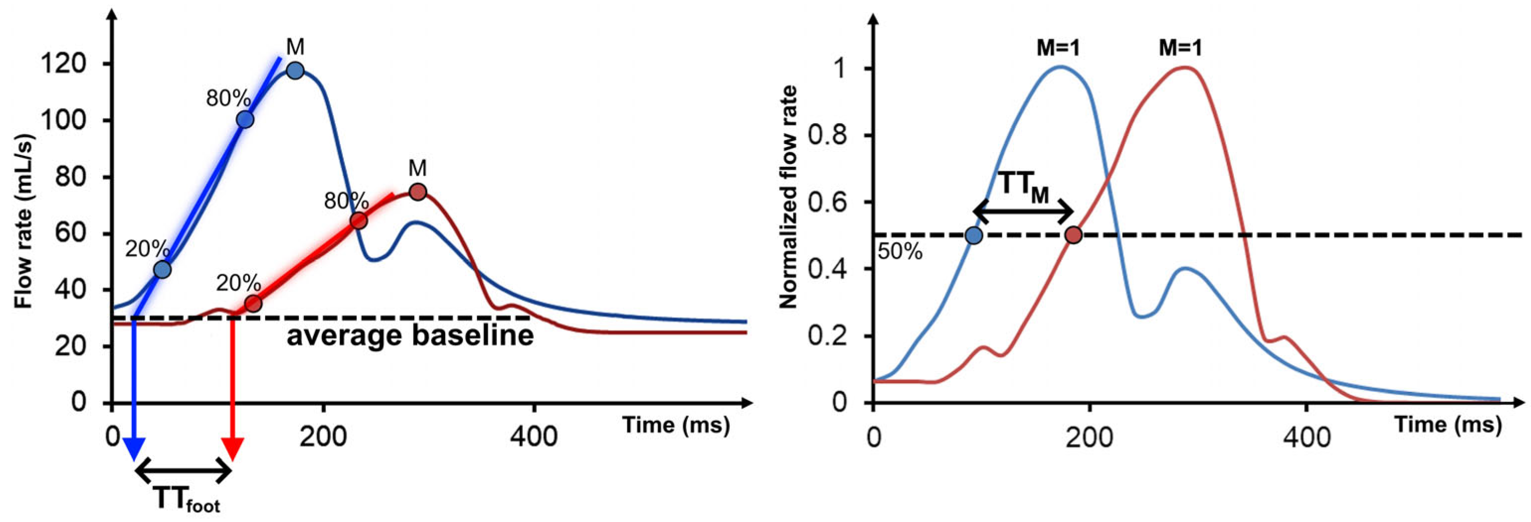
PWV was estimated from flow rate curves obtained in the benchtop experiments, in the simulation and using 2D- and 4D-Flow acquisitions along the aortic centerline. In the 1D simulation, planes were placed every 10 mm and in the lab every ≈50 mm. Net flow rates were assessed with 2D-Flow along planes orthogonal to the aortic lumen every 40 mm (10 planes for model #1 and 13 planes for model #2) and every 5 mm using 4D-Flow. Different methods have been proposed to estimate PWV using MRI flow rate curves [15,16]. Globally, PWV is computed using the linear distances along the aortic centerline between the center of the planes used for flow rate estimation and the corresponding transit time (TT). As shown in Figure 3, two different TT algorithms were implemented in our study [15]: median method (TTM) and foot method (TTfoot). For both the TTM and TTfoot estimations, the maximum (peak) and minimum (baseline) flow rate values were first automatically identified across all curves. For TTM, the point of interest occurs when the flow rate upstroke reaches 50% of its maximum. The TTM for each waveform was computed as the difference between its 50% time point and that of the inlet flow rate. For TTfoot, all points in the flow rate upstroke between 20% and 80% were fitted to a straight line by least squares regression. The time at which this line intersected the mean baseline value of all the flow rate curves was defined as the foot of the curve. The TTfoot for each waveform was then computed as the difference between its foot and that of the inlet waveform. The inverse of the linear regression slope between flow transit times and plane distances for the entire aorta was used to estimate PWV. A regional PWV for the thoracic aorta (first 200 mm from the inlet) was also calculated for the 4D-Flow acquisition.

3. Results

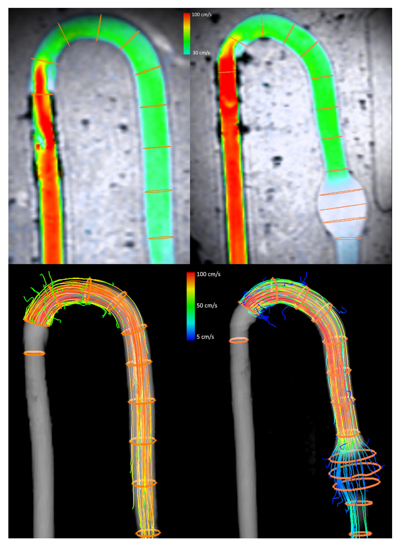
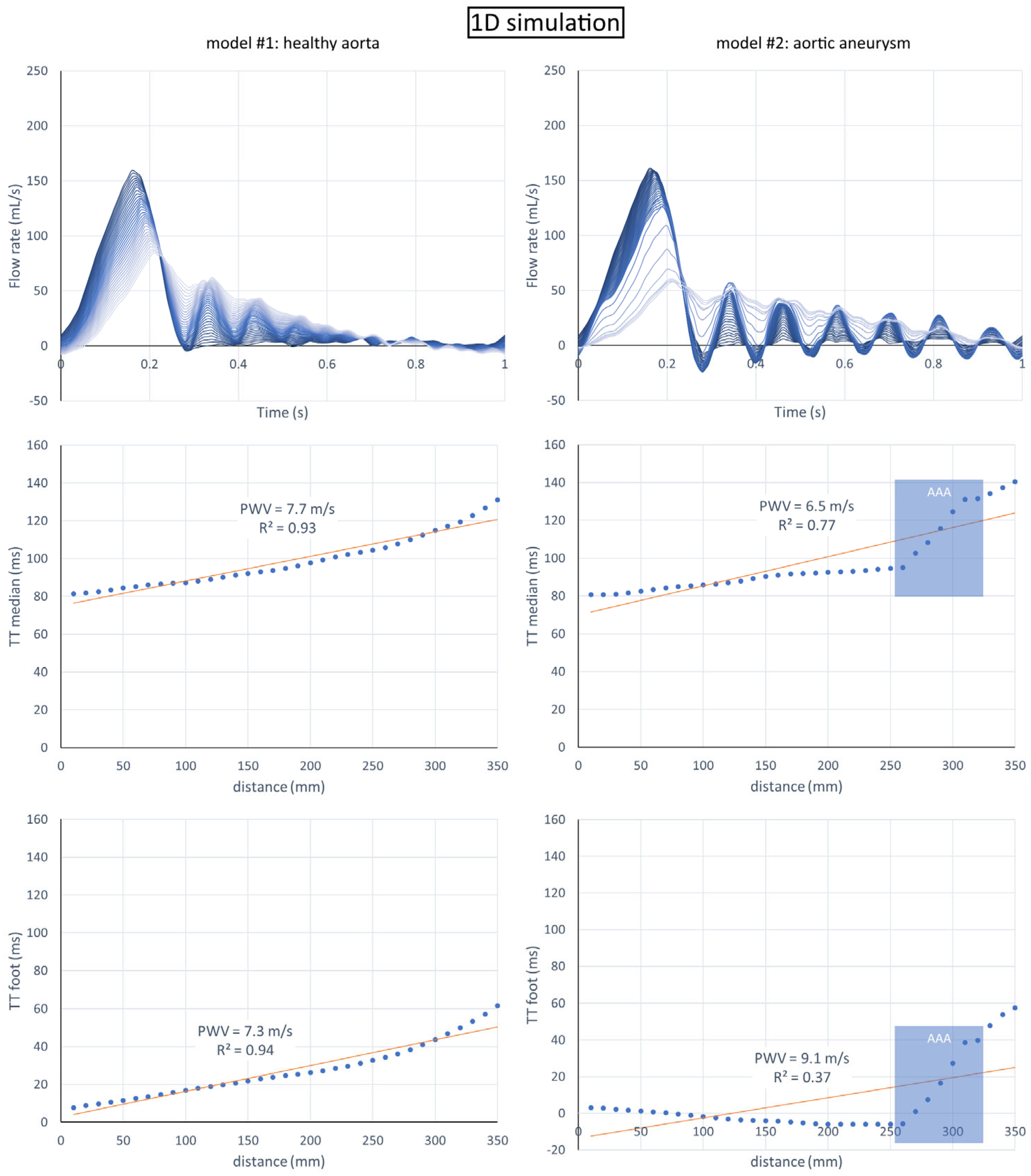
The circulatory system reproduced maximum flow velocities of ≈1 m/s in the ascending aorta, which decreased toward the periphery, particularly within the dilated region in model #2 (Figure 4, Video S1 and Video S2). The 1D simulation results of the flow rate along the aorta in each model and the PWV estimates are presented in Figure 5. In the healthy aorta, a decrease in peak flow and an almost linear increase in transit time from the inlet toward the outlet can be observed. The PWV was 7.7 m/s (SE = 0.31 m/s, r2 = 0.93) using TTM and 7.3 m/s (SE = 0.34 m/s, r2 = 0.94) with TTfoot. In the AAA model, the maximum flow remained elevated in the region proximal to the dilation and decreased rapidly within and beyond the aneurysm. Accordingly, transit times remained stable in the proximal region and increased steadily from the dilated segment, resulting in PWV values of 6.5 m/s (SE = 0.49 m/s, r2 = 0.77) and 9.1 m/s (SE = 0.80 m/s, r2 = 0.37) for the TTM and TTfoot methods, respectively. Considering only the thoracic region, the stable transit time values obtained with the TTM method would result in a higher apparent PWV value. Furthermore, the TTfoot method produced a negative slope with negative transit time values, showing the effects of backward flow waves observed on the upstroke flow rate, which could produce apparent non-physiological transit time values. As a reference, the theoretical PWV using the M-K equation for model #1 was 6.8 m/s.
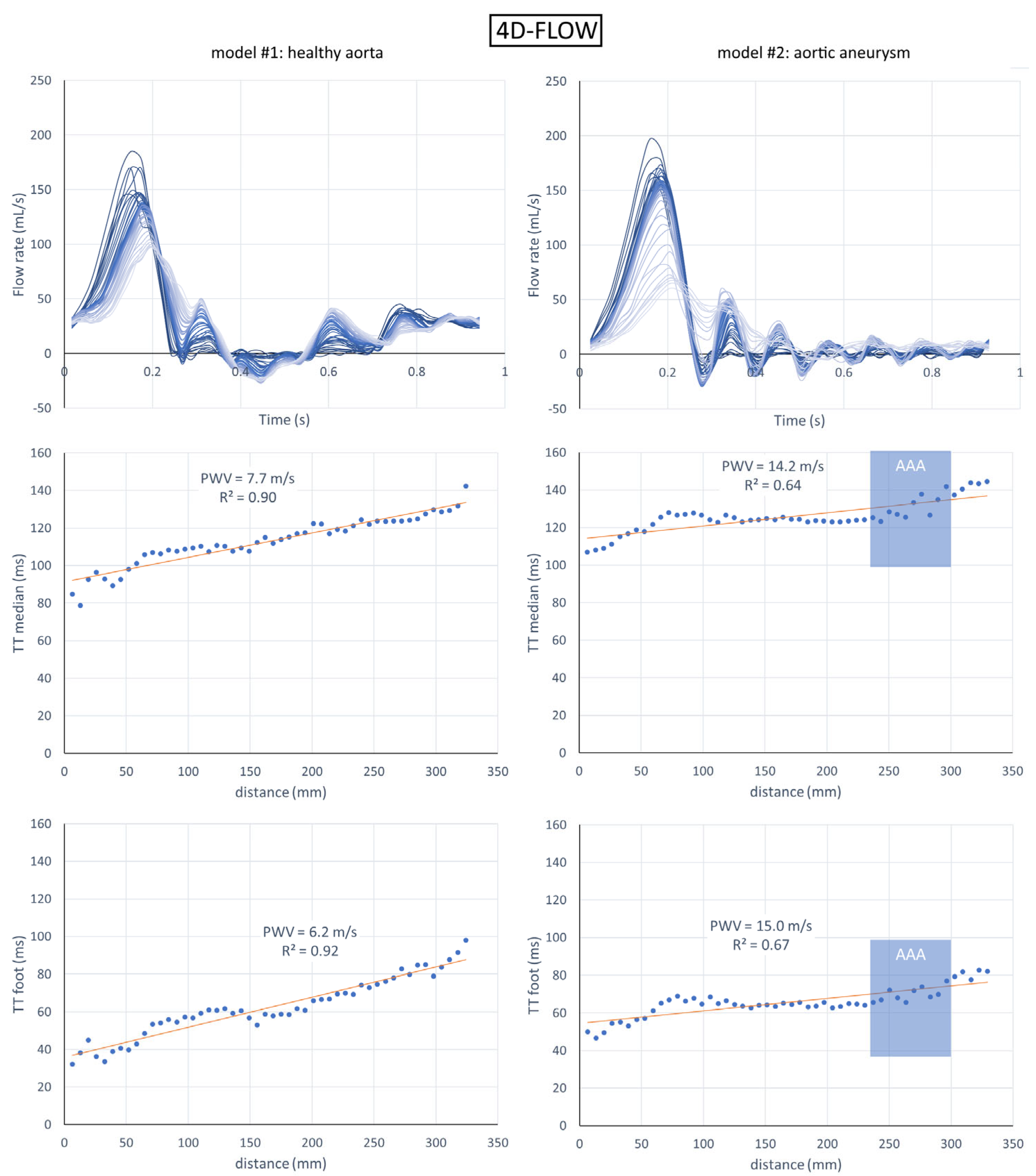
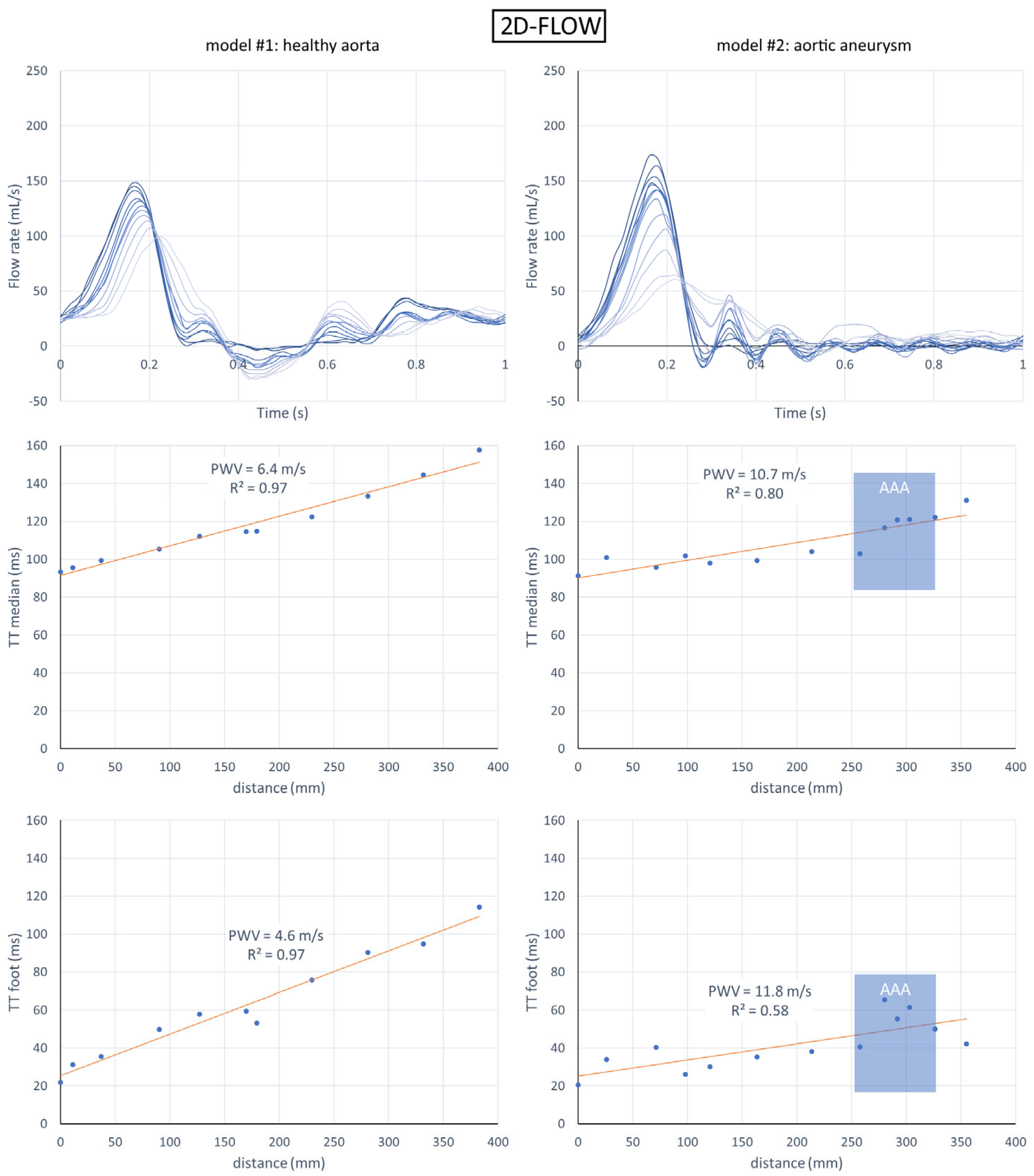
Following the same presentation format, the flow curves and PWV estimates for the 4D-Flow and 2D-Flow measurements are shown in Figure 6 and Figure 7, respectively. As in the simulation, in model #1 the maximum flow rate decreased along the aorta, while it remained more stable in model #2 in the thoracic aorta and then decreased rapidly. The linear relationship between TT and distance yielded PWV values for the healthy aorta of 7.7 m/s (SE = 0.33 m/s, r2 = 0.90) and 6.2 m/s (SE = 0.24 m/s, r2 = 0.90) using the TTM and TTfoot methods, respectively. Dilation in the abdominal region produced a marked flattening of the regression curve and consequent elevated PWV values that reached 14.2 m/s (SE = 0.98 m/s, r2 = 0.64) using TTM and 15.0 m/s (SE = 1.02 m/s, r2 = 0.67) with TTfoot. The correlation coefficients were lower in the diseased than in the healthy aorta model. The regional PWV for the first 200 mm of the thoracic aorta segment was 15.7 m/s (SE = 1.44 m/s, r2 = 0.41) using TTM and 15.3 m/s (SE = 1.40 m/s, r2 = 0.44) with TTfoot. When performing 2D-Flow measurements, the number of planes was limited to 11 locations, but the behavior was similar to that observed using 4D-Flow measurements, although PWV values were lower (Figure 7). For model #1, the PWV was 6.4 m/s (SE = 0.36 m/s, r2 = 0.97) using TTM and 4.6 m/s (SE = 0.27 m/s, r2 = 0.94) with TTfoot and for model #2 these were 10.7 m/s (SE = 1.29 m/s, r2 = 0.80) and 11.8 m/s (SE = 1.75 m/s, r2 = 0.58), respectively. The mean area of the ROIs in the thoracic aorta segment was 380 mm2, corresponding to an average diameter of 22 mm.
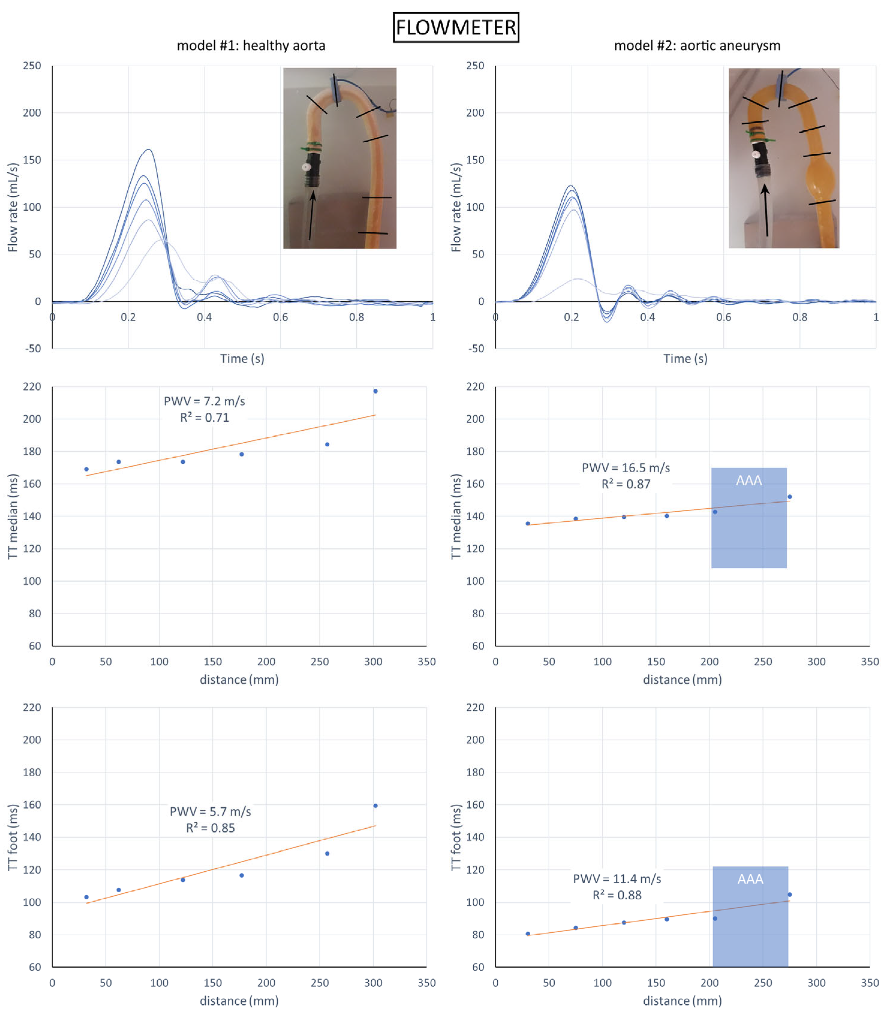
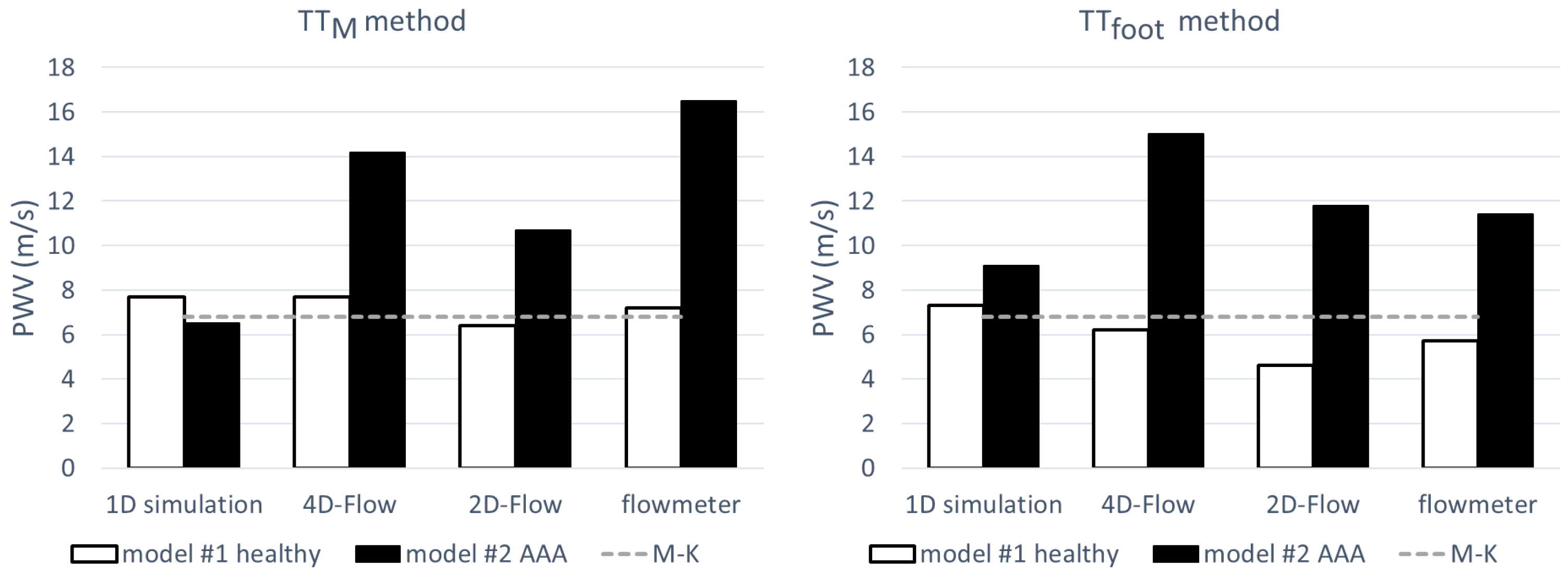
Finally, in the laboratory, flow and distance were measured at only six locations along the aorta (Figure 8). The behavior in the flow curves followed a pattern similar to that described above. For model #1, the PWV was 7.2 m/s (SE = 1.64 m/s, r2 = 0.71) using TTM and 5.7 m/s (SE = 1.02 m/s, r2 = 0.94) with TTfoot. For model #2, the relationship between TT and distance showed a less pronounced slope, with PWV values of 16.5 m/s (SE = 2.16 m/s, r2 = 0.87) and 11.4 m/s (SE = 1.61 m/s, r2 = 0.88) using TTM and TTfoot, respectively. PWV values for all measurements and methods are shown in Figure 9.
Maximum and minimum pressure values measured before the MRI acquisition in the aortic outlet (P2, Figure 2) for model #1 were 48 and 32 mmHg. Maximum and minimum pressure values for model #2 were 45 and 32 mmHg, respectively.

4. Discussion

This in vitro experimental study compared two initially identical aortas with the same wall elasticity, and the addition of an abdominal aneurysm resulted in a twofold increase in PWV measured with 4D-Flow. This behavior was observed under ideal controlled conditions and using a standard 4D-Flow acquisition, in two aortas constructed from the same latex, with constant wall thickness and no bifurcations or tapering. The reflections produced by the aneurysm significantly affected the amplitude of the flow rate curves all along the thoracic aorta. These findings suggest that indirect measurements of thoracic aortic stiffness based on PWV in the presence of abdominal aortic aneurysms should consider the impact of reflections caused by dilation.
The main finding of this in vitro study, which compared PWV measured using 4D-Flow between a healthy aorta and an aorta with an abdominal aneurysm, but with identical wall thicknesses and elasticity, is that the PWV doubled in the dilated aorta compared to the healthy model. This result was confirmed using two methods typically employed to estimate transit times between flow rate curves in 4D-Flow [15,16,27]. The first method was based on the time-to-foot, which was calculated using a regression line between 20% and 80% of the flow curve, and the second on the time to reach 50% of peak flow.
In the healthy model, transit time increased linearly with distance, yielding PWV estimates between 6 and 8 m/s. In contrast, in the dilated model, the relationship was flatter, with shorter transit times in the thoracic region and a consequent increase in PWV to values between 14 and 15 m/s. This effect is likely due to the reflections produced by the dilation, as observed in the flow rate curves. In a healthy aorta, peak flow decreases evenly from the ascending aorta towards the abdominal region, probably due to a reflected flow wave caused by a distal impedance mismatch. The mechanical coupling between the compliant latex aorta and the rigid silicone tube at the end of the abdominal segment causes considerable elastic mismatch, which is only partially minimized by the compliant windkessel chamber. This elastic mismatch produces a reflected flow wave that directly impacts the systolic peak, an effect that is clearly evident in the numerical simulation. Dilation produces the exact opposite effect, generating a positive flow wave that adds to the incident flow, thereby enhancing the flow peak rather than reducing it. In other words, the abdominal aneurysm creates a suction that draws fluid inward. Thus, in model #2, the mentioned decrease in the maximum flow amplitude was less evident in the thoracic region, where the flow curves superposed and transit times shortened. Previous reports have accurately described this phenomenon in laboratory experiments, although they employed long tubes that minimized the overlap of reflected and incident waves at the flow curve upstroke [18]. For physiologically realistic aortic sizes and lengths, such as those in our study, the reflected waves produced by an abdominal aneurysm quickly reach the flow upstroke curve and interfere with it all along the thoracic aorta. In essence, even in a controlled environment with a non-bifurcated aorta and linear, constant-thickness aortic wall elasticity, the abdominal aneurysm produced reflected waves that likely contaminated the ascending phase of the flow curve and altered the correlation between PWV and the level of arterial stiffness. This occurred throughout the entire thoracic region, as anticipated in the numerical simulation, and confirmed in both the 2D-Flow acquisitions and laboratory measurements. In an extreme case of the 1D simulation, the TTfoot method produced non-physiological negative transit time values, as shown in the bottom row of Figure 5 for model #2. This behavior suggests that the apparent PWV, as estimated from the regression between transit times and distances, should not be directly associated with a measurement of arterial elasticity without first considering the reflections resulting from dilatations.
Attempts have previously been made to use PWV measurements obtained using 4D-Flow to estimate aortic stiffness in an in vitro model. The M-K equation, which relates PWV to arterial elasticity, has been validated in vitro using ultrasound flow measurements and 4D-Flow MRI in short, straight, homogeneous segments [15,28]. Recently, Zimmermann et al. [17] studied patient-specific silicone aortas of varying stiffness using 4D-Flow and observed an increase in PWV in the stiffer models, though the theoretical values based on the M-K equation were not achieved. The authors explain that these theoretical values should be debated because they assume ideal conditions and the absence of reflections. The M-K equation relates true wave speed to wall elasticity, but it only applies under ideal conditions to an infinite tube in the absence of reflections. In the presence of reflected waves induced by an aortic aneurysm, only an apparent PWV can be obtained from TT–distance regression. Our in vitro study shows that, in two models with equal, constant aortic wall thickness and elasticity, the presence of an AAA produces reflections that alter this apparent PWV compared to a healthy aorta. Other groups have worked with in vitro systems and 4D-Flow to study aortic coarctations [14], but none have studied the impact of abdominal aneurysms on PWV in such experimental setups. The effect of reflected waves caused by abdominal aneurysms has been studied in in vitro laboratory models and numerical simulations [29], which confirm the existence of an expansive reflected wave produced by dilation. While numerous studies have reported on various methods for separating incident and reflected waves using 4D-Flow, these strategies typically require a reflection-free region, which is beyond the scope of this study [26,30,31].
Recent advances in MRI techniques have made it possible to accurately study aortic stiffness in the presence of aortic disease, providing more information than anatomical measurements obtained using computed tomography [8,32]. The 4D-Flow MRI sequence, in particular, has proven effective in estimating the global PWV of the aorta [33] and quantifying changes in elasticity associated with aging and across different aortic segments [34,35]. However, when the aorta undergoes significant geometric changes, such as the dilation observed in AAA, the relationship between PWV and arterial stiffness can be impaired. In patients with bicuspid valves, it was reported that dilation of the ascending aorta did not produce the expected increase in PWV [10]. In subjects with AAA, pulse wave velocity measured by MRI has been reported to increase only in the thoracic region and not in the abdominal region [36]. A more recent 4D-Flow study showed the opposite, opening a debate regarding the effect of AAA on PWV assessment [37,38]. Our results demonstrate that the presence of an abdominal aneurysm hampers the direct correlation between PWV and stiffness. This does not mean that there are no alternative imaging techniques for estimating aortic stiffness in the presence of dilations. Using 4D-Flow MRI, wall shear stress could be estimated and was associated with regions vulnerable to rupture [39,40]. Ultrasound measurements of distensibility in the dilated region have shown that they can complement geometric measurements, improving the prediction of rupture [41,42]. It has been reported that detailed estimation of the aneurysm geometry and wall thickness using CT imaging can potentially improve diagnoses [43]. Although there are methods for estimating arterial stiffness based on the initial slope of the flow-area loop, these approaches are only valid when the upstroke of the waves is not affected by reflections [30]. Finally, PWV can also be estimated non-invasively using medical devices adapted for routine clinical use. Based on PWV measurements obtained using arterial tonometry, improvements in the prediction of the expansion of thoracic aortic aneurysms were reported, beyond the risks calculated based on maximum diameter [44]. However, another study found similar PWV values between patients with dilated aortas vs non-aortic vascular disease or even between treated vs non-treated subjects with aortic aneurysms [45]. These results highlight the complex relationship between apparent PWV and arterial elasticity in patients with aortic aneurysms.
This study has some identified limitations. The aortic models did not include supra-aortic vessels and were designed without tapering to avoid additional sources of wave reflection. Under the current simplified conditions, the relationship between PWV and elasticity has already been altered by reflections resulting from elastic mismatch and AAA. Therefore, both bifurcations and tapering would only amplify this effect. Additionally, all tests were conducted under pressure conditions that were below physiological levels. However, we believe this has little impact since latex behaves linearly within the studied pressure-strain range. The experiments were conducted using water flow, which has a lower viscosity than blood. However, preliminary 1D simulations with a fluid of higher viscosity did not reveal any significant differences in wave reflection. Latex was used to fabricate the compliant models, despite the fact that the aortic wall elasticity is non-linear. While we acknowledge that models with non-linear elasticity could be created, and that more sophisticated methods exist for fabricating flexible abdominal aneurysm models [46], these methods were beyond the scope of this study. These limitations do not undermine the applicability of the results obtained in the controlled in vitro design, which highlight that, when comparing two aortic models with the same wall thickness and elasticity, the presence of aortic dilatation produces an apparent PWV that is not related to arterial stiffness. The experiment included only one AAA model to demonstrate the impact of dilation on PWV estimation, although aneurysms of a different shape/size could be designed and tested in future studies. We prioritized conducting a single experiment on the same day with both a healthy and a dilated model to specifically compare the effect of dilatation on PWV assessment. Moreover, only two methods were used to estimate transit times, even though other alternatives are available [16]. However, the transit time shortening observed in model #2 with the AAA adequately reflected the overlap between flow curves in the thoracic aorta and would not be expected to be significantly affected by the use of alternative methods. Finally, the 4D-Flow sequence has the advantage of enabling flow measurements across a greater number of planes than the 2D-Flow sequence, but it has the disadvantage of lower spatial and temporal resolution. The spatial and temporal resolution of our 4D-Flow acquisition remained within the recommended values [17], and we observed no significant differences in PWV compared to higher-resolution 2D-Flow measurements.

5. Conclusions

PWV is a surrogate of arterial stiffness that depends on the geometry of the vessels. In this in vitro study, PWV assessed using 4D-Flow MRI was compared between a healthy and a dilated aorta, both having the same elasticity and wall thickness. PWV values doubled in the dilated aorta, mostly due to the impact of reflections observed throughout the thoracic segment. Therefore, the effect of reflections must be considered when attempting to estimate arterial stiffness using PWV in the presence of abdominal aneurysms.

Supplementary Materials

The following supporting information can be downloaded at: https://www.mdpi.com/article/10.3390/fluids11070177/s1, Video S1: Velocity streamlines in healthy aorta (model #1), Video S2: Velocity streamlines in aorta with an abdominal aneurysm (model #2).

Author Contributions

Conceptualization, D.C., M.E.C. and E.E.R.; methodology, D.C., E.E.R. and A.V.; software, D.C., M.E.C., E.L. and S.S.; validation, E.E.R., E.L. and S.S.; formal analysis, D.C., M.E.C., E.L., S.S., E.E.R. and A.V.; investigation, D.C., E.E.R., S.G. and E.C.F.; resources, D.C., E.E.R. and A.V.; data curation, D.C., E.L. and S.S.; writing—original draft preparation, D.C., M.E.C. and E.E.R.; writing—review and editing, D.C., M.E.C., E.E.R., A.V., E.C.F. and S.G.; visualization, D.C., M.E.C., E.E.R., E.L. and S.S. All authors have read and agreed to the published version of the manuscript.

Funding

This research was partly funded by FONCYT-ANPCYT project PICT 2019 Nº1563 (Argentina), by the 2024 Florencio Fiorini Grant for Biomedical Science Research, and 2023 Grant for Strengthening Research Projects (Universidad Nacional de General Sarmiento, Argentina).

Institutional Review Board Statement

Not applicable.

Informed Consent Statement

Not applicable.

Data Availability Statement

The data cannot be made publicly available upon publication because they are not available in a format that is sufficiently accessible or reusable by other researchers. The data that support the findings of this study are available upon reasonable request from the authors.

Acknowledgments

We would like to thank Diego Campana, dean of the Faculty of Engineering at the National University of Entre Ríos, for helping us obtain the flowmeter used during the laboratory experiments. We also thank Analia Martino, Sabrina Defeo, Romina Boggio, Ariel Martinez, Valentina Stipechi, Federico Scapellato and Pablo Cornes for their invaluable effort during the phantom experiments.

Conflicts of Interest

The authors declare no conflicts of interest.

Abbreviations

The following abbreviations are used in this manuscript:
AAAAbdominal aortic aneurysm
ECGElectrocardiogram
MRIMagnetic resonance imaging
PWVPulse wave velocity
M-KMoens–Korteweg
TTTransit-time
CFLCourant–Friedrichs–Lewy number
ROIRegion of interest
FOVField of view

Appendix A

Numerical Method to Calculate Flow

A 4D-Flow study corresponds to a four-dimensional vector field, where each voxel contains information about the anatomical representation or magnitude image and the velocity components in the anterior–posterior (vap), left–right (vlr), and superior–inferior (vsi) directions. With this information, it is possible to reconstruct a velocity vector v(x,t) = (vap(x,t),vlr(x,t),vsi(x,t)) at any 3D position x within the volume by applying a trilinear interpolation; for any time phase t [22], the user interactively positions an observation plane perpendicular to the aorta through an interactive multiplanar reconstruction using cursors that allow the translation and rotation of orthogonal views, centered on the vessel at different anatomical levels. This observation plane is also used as a sampling grid for the velocity vector and is internally composed of square pixels with a side length of s = 0.5 mm. This grid is perpendicular to a unit normal vector n that defines its orientation. On this observation plane, the user creates an ROI by manually placing points around the vessel cross-sectional area that are interpolated with a Catmull–Rom cubic spline to create a smooth and closed curve. As explained in [22], all pixels lying inside the ROI, with positions xROI, are used for flow computation. For example, net flow Qnet is calculated for any time phase t using the following expression:
Q n e t t = x x R O I v x , t · n · s 2
where n is the unitary normal vector of the observation plane. In some regions of the ascending aorta, the vessel pulsates in such a way that a single ROI cannot contain the entire cross-sectional area of the vessel throughout the cardiac cycle (due to factors such as systolic expansion and/or displacement). In these cases, the user can select multiple ROIs over the same observation plane, typically one at systole and one at diastole. This makes it possible to linearly interpolate the contours of the two ROIs to achieve a smooth transition. The impact of ROI angulation, resolution and size has been reported previously [22].

Appendix B

Details of 1D-Flow Simulation
Assuming no fluid loss through the arterial wall, the governing equations for a one-dimensional (1D) incompressible flow are written as [23,24]:
A t + A v z = 0 v t + v v z + 1 ρ p z = f
where A is the vessel cross-sectional area, v is the flow velocity, p is the pressure, ρ is the fluid density, f represents the viscous friction force per unit volume, t denotes time and z is the axial coordinate. Under the assumption of laminar flow, the viscous friction force per unit volume is given by:
f = 8 π μ ρ · v A
with μ denoting the fluid dynamic viscosity.
Transforming system (A2) into its characteristic form leads to the following compatibility equation [23]:
d v ± d p ρ · c = f v · c A A z p d t
along the characteristic paths dz/dt = v ± c, where c is the characteristic velocity (i.e., the local wave speed) defined as:
c = A ρ p A z
In order to close the system, a constitutive relation (or state equation) of the form p = p(A) is applied. In this study, the equation of state proposed by Absi [25] is used, given by:
p p e x t = E · h r 0 ( 1 ν 2 ) A 0 A 1 A 0 A
where pext is the external pressure on the vessel, A0 is the vessel cross-sectional area when p = pext, with r0 being the corresponding inner radius, h is the vessel wall thickness, E is the Young’s modulus of the vessel wall, and v is its Poisson’s ratio.
The numerical solution is carried out by discretizing the 1D domain into N elements and assuming the solution known at time tn. The discrete versions of the compatibility equations are solved for time tn+1 subject to the constraint Δz = (v ± c)Δt, where Δt = tn+1 − tn and both the flow and characteristic speeds are evaluated at tn. The maximum allowable Δt must satisfy the CFL condition, expressed as max{(vn ± cn) Δt/Δzmesh} < 1, with Δzmesh representing the length of the mesh elements. For a given mesh point i at time tn+1, the flow variables are linearly interpolated at the foot of the characteristic, located at the axial coordinate zs = zi − (vn ± cn)· Δt and time tn, in order to define the differences Δv = vin+1 − vsn and Δp = pin+1 − psn. Figure A1 shows the characteristics of the numerical simulations performed to emulate model #1 and model #2.
Figure A1. Design characteristics of models for (a) the healthy aorta (model #1) and (b) the aorta with an abdominal aneurysm (model #2).
Fluids 11 00177 g0a1

References

  1. Schanzer, A.; Oderich, G.S. Management of abdominal aortic aneurysms. N. Engl. J. Med. 2021, 385, 1690–1698. [Google Scholar] [CrossRef] [Scilit] [PubMed]
  2. Members, W.C.; Isselbacher, E.M.; Preventza, O.; Hamilton Black, J., III; Augoustides, J.G.; Beck, A.W.; Bolen, M.A.; Braverman, A.C.; Bray, B.E.; Brown-Zimmerman, M.M. 2022 ACC/AHA guideline for the diagnosis and management of aortic disease: A report of the American Heart Association/American College of Cardiology Joint Committee on Clinical Practice Guidelines. J. Am. Coll. Cardiol. 2022, 80, e223–e393. [Google Scholar]
  3. Anagnostakos, J.; Lal, B.K. Abdominal aortic aneurysms. Prog. Cardiovasc. Dis. 2021, 65, 34–43. [Google Scholar] [CrossRef] [Scilit] [PubMed]
  4. Ren, S.; Guidoin, R.; Xu, Z.; Deng, X.; Fan, Y.; Chen, Z.; Sun, A. Narrative review of risk assessment of abdominal aortic aneurysm rupture based on biomechanics-related morphology. J. Endovasc. Ther. 2024, 31, 178–190. [Google Scholar] [PubMed]
  5. Laurent, S.; Boutouyrie, P.; Asmar, R.; Gautier, I.; Laloux, B.; Guize, L.; Ducimetiere, P.; Benetos, A. Aortic stiffness is an independent predictor of all-cause and cardiovascular mortality in hypertensive patients. Hypertension 2001, 37, 1236–1241. [Google Scholar] [CrossRef] [Scilit] [PubMed]
  6. Reference Values for Arterial Stiffness’ Collaboration. Determinants of pulse wave velocity in healthy people and in the presence of cardiovascular risk factors: ‘Establishing normal and reference values’. Eur. Heart J. 2010, 31, 2338–2350. [CrossRef] [Scilit] [PubMed]
  7. Dushfunian, D.; Cohn, S.; Berhane, H.; Markl, M. 4D Flow MRI of the Thoracic Aorta. Radiol. Cardiothorac. Imaging 2025, 7, e240532. [Google Scholar] [CrossRef] [Scilit] [PubMed]
  8. Wentland, A.L.; Grist, T.M.; Wieben, O. Review of MRI-based measurements of pulse wave velocity: A biomarker of arterial stiffness. Cardiovasc. Diagn. Ther. 2014, 4, 193–206. [Google Scholar] [PubMed]
  9. Pai, R.G.; Shah, P.M. Relationship between the pulse wave and the flow velocity wave and their propagation velocities in the arterial system: Implications for the assessment of regional physical properties of the arterial beds. Int. J. Angiol. 1999, 8, 127–130. [Google Scholar] [CrossRef] [Scilit]
  10. Pascaner, A.F.; Houriez, S.; Craiem, D.; Gencer, U.; Casciaro, M.E.; Charpentier, E.; Bouaou, K.; De Cesare, A.; Dietenbeck, T.; Chenoune, Y. Comprehensive assessment of local and regional aortic stiffness in patients with tricuspid or bicuspid aortic valve aortopathy using magnetic resonance imaging. Int. J. Cardiol. 2021, 326, 206–212. [Google Scholar] [CrossRef] [Scilit] [PubMed]
  11. Koskas, L.; Doizi, S.; Parmentier, E.; Bakir, F.; Davaine, J.-M. Use of Phantoms to Enhance Mechanical Knowledge About Aortic Aneurysms: A Systematic Review. J. Biomech. Eng. 2025, 147, 120802. [Google Scholar] [CrossRef] [Scilit] [PubMed]
  12. Jeong, J.-H.; Lee, B.; Hong, J.; Yang, T.-H.; Park, Y.-H. Reproduction of human blood pressure waveform using physiology-based cardiovascular simulator. Sci. Rep. 2023, 13, 7856. [Google Scholar] [CrossRef] [Scilit] [PubMed]
  13. Vignali, E.; Gasparotti, E.; Mariotti, A.; Haxhiademi, D.; Ait-Ali, L.; Celi, S. High-versatility left ventricle pump and aortic mock circulatory loop development for patient-specific hemodynamic in vitro analysis. ASAIO J. 2022, 68, 1272–1281. [Google Scholar] [CrossRef] [Scilit] [PubMed]
  14. Urbina, J.; Sotelo, J.A.; Springmüller, D.; Montalba, C.; Letelier, K.; Tejos, C.; Irarrázaval, P.; Andia, M.E.; Razavi, R.; Valverde, I. Realistic aortic phantom to study hemodynamics using MRI and cardiac catheterization in normal and aortic coarctation conditions. J. Magn. Reson. Imaging 2016, 44, 683–697. [Google Scholar] [CrossRef] [Scilit] [PubMed]
  15. Ruesink, T.; Medero, R.; Rutkowski, D.; Roldan-Alzate, A. In vitro validation of 4D flow MRI for local pulse wave velocity estimation. Cardiovasc. Eng. Technol. 2018, 9, 674–687. [Google Scholar] [CrossRef] [Scilit] [PubMed]
  16. Houriez–Gombaud-Saintonge, S.; Mousseaux, E.; Bargiotas, I.; De Cesare, A.; Dietenbeck, T.; Bouaou, K.; Redheuil, A.; Soulat, G.; Giron, A.; Gencer, U. Comparison of different methods for the estimation of aortic pulse wave velocity from 4D flow cardiovascular magnetic resonance. J. Cardiovasc. Magn. Reson. 2019, 21, 75. [Google Scholar] [CrossRef] [Scilit] [PubMed]
  17. Zimmermann, J.; Loecher, M.; Kolawole, F.O.; Bäumler, K.; Gifford, K.; Dual, S.A.; Levenston, M.; Marsden, A.L.; Ennis, D.B. On the impact of vessel wall stiffness on quantitative flow dynamics in a synthetic model of the thoracic aorta. Sci. Rep. 2021, 11, 6703. [Google Scholar] [CrossRef] [Scilit] [PubMed]
  18. Hacham, W.S.; Khir, A.W. The speed, reflection and intensity of waves propagating in flexible tubes with aneurysm and stenosis: Experimental investigation. Proc. Inst. Mech. Eng. Part H J. Eng. Med. 2019, 233, 979–988. [Google Scholar] [CrossRef] [Scilit]
  19. Casciaro, M.E.; Craiem, D.; Chironi, G.; Graf, S.; Macron, L.; Mousseaux, E.; Simon, A.; Armentano, R.L. Identifying the principal modes of variation in human thoracic aorta morphology. J. Thorac. Imaging 2014, 29, 224–232. [Google Scholar] [CrossRef] [Scilit] [PubMed]
  20. Rodríguez, E.E.; Valda, A.; Casciaro, M.E.; Graf, S.; Fischer, E.C.; Craiem, D. Accuracy of flow volume estimation in the dilated aorta using 4D flow MRI: A pulsatile phantom study. Physiol. Meas. 2025, 46, 015006. [Google Scholar] [CrossRef] [Scilit]
  21. Craiem, D.; Pascaner, A.F.; Casciaro, M.E.; Gencer, U.; Alcibar, J.; Soulat, G.; Mousseaux, E. Automatic correction of background phase offset in 4D-flow of great vessels and of the heart in MRI using a third-order surface model. Magn. Reson. Mater. Phys. Biol. Med. 2019, 32, 629–642. [Google Scholar] [CrossRef] [Scilit]
  22. Casciaro, M.E.; Pascaner, A.F.; Guilenea, F.N.; Alcibar, J.; Gencer, U.; Soulat, G.; Mousseaux, E.; Craiem, D. 4D flow MRI: Impact of region of interest size, angulation and spatial resolution on aortic flow assessment. Physiol. Meas. 2021, 42, 035004. [Google Scholar] [CrossRef] [Scilit]
  23. Anliker, M.; Rockwell, R.L.; Ogden, E. Nonlinear analysis of flow pulses and shock waves in arteries: Part I: Derivation and properties of mathematical model. Z. Angew. Math. Phys. ZAMP 1971, 22, 217–246. [Google Scholar] [CrossRef] [Scilit]
  24. Olufsen, M.S. Structured tree outflow condition for blood flow in larger systemic arteries. Am. J. Physiol.-Heart Circ. Physiol. 1999, 276, H257–H268. [Google Scholar] [CrossRef] [Scilit]
  25. Absi, R. Revisiting the pressure-area relation for the flow in elastic tubes: Application to arterial vessels. Ser. Biomech. 2018, 32, 47–59. [Google Scholar]
  26. Hughes, A.D.; Parker, K.H. Forward and backward waves in the arterial system: Impedance or wave intensity analysis? Med. Biol. Eng. Comput. 2009, 47, 207–210. [Google Scholar] [CrossRef] [Scilit] [PubMed]
  27. Wang, B.; Sun, A.; Li, H.; Chen, Z.; Cao, R.; Li, H.; Chu, Y.H.; Jin, N.; Wang, H. Highly Accelerated Aortic 4D Flow MRI: Implications for Pulse Wave Velocity Measurements. J. Magn. Reson. Imaging 2026, 63, 549–560. [Google Scholar] [PubMed]
  28. Shahmirzadi, D.; Li, R.X.; Konofagou, E.E. Pulse-wave propagation in straight-geometry vessels for stiffness estimation: Theory, simulations, phantoms and in vitro findings. J. Biomed. Eng. 2012, 134, 114502. [Google Scholar] [CrossRef] [Scilit]
  29. Swillens, A.; Lanoye, L.; De Backer, J.; Stergiopulos, N.; Verdonck, P.R.; Vermassen, F.; Segers, P. Effect of an abdominal aortic aneurysm on wave reflection in the aorta. IEEE Trans. Biomed. Eng. 2008, 55, 1602–1611. [Google Scholar] [CrossRef] [PubMed]
  30. Feng, J.; Khir, A. Determination of wave speed and wave separation in the arteries using diameter and velocity. J. Biomech. 2010, 43, 455–462. [Google Scholar] [CrossRef] [Scilit] [PubMed]
  31. Biglino, G.; Steeden, J.A.; Baker, C.; Schievano, S.; Taylor, A.M.; Parker, K.H.; Muthurangu, V. A non-invasive clinical application of wave intensity analysis based on ultrahigh temporal resolution phase-contrast cardiovascular magnetic resonance. J. Cardiovasc. Magn. Reson. 2012, 14, 65. [Google Scholar] [CrossRef] [Scilit]
  32. Whitlock, M.C.; Hundley, W.G. Noninvasive imaging of flow and vascular function in disease of the aorta. JACC Cardiovasc. Imaging 2015, 8, 1094–1106. [Google Scholar] [CrossRef] [Scilit] [PubMed]
  33. Markl, M.; Wallis, W.; Brendecke, S.; Simon, J.; Frydrychowicz, A.; Harloff, A. Estimation of global aortic pulse wave velocity by flow-sensitive 4D MRI. Magn. Reson. Med. Off. J. Int. Soc. Magn. Reson. Med. 2010, 63, 1575–1582. [Google Scholar] [CrossRef] [Scilit]
  34. Harloff, A.; Mirzaee, H.; Lodemann, T.; Hagenlocher, P.; Wehrum, T.; Stuplich, J.; Hennemuth, A.; Hennig, J.; Grundmann, S.; Vach, W. Determination of aortic stiffness using 4D flow cardiovascular magnetic resonance-a population-based study. J. Cardiovasc. Magn. Reson. 2018, 20, 43. [Google Scholar] [CrossRef] [Scilit] [PubMed]
  35. Soulat, G.; Gencer, U.; Kachenoura, N.; Villemain, O.; Messas, E.; Boutouyrie, P.; Laurent, S.; Mousseaux, E. Changes in segmental pulse wave velocity of the thoracic aorta with age and left ventricular remodelling. An MRI 4D flow study. J. Hypertens. 2020, 38, 118–126. [Google Scholar] [CrossRef] [Scilit] [PubMed]
  36. Abbas, A.; Cecelja, M.; Hussain, T.; Greil, G.; Modarai, B.; Waltham, M.; Chowienczyk, P.J.; Smith, A. Thoracic but not abdominal phase contrast magnetic resonance-derived aortic pulse wave velocity is elevated in patients with abdominal aortic aneurysm. J. Hypertens. 2015, 33, 1032–1038. [Google Scholar] [CrossRef] [Scilit] [PubMed]
  37. Lindenberger, M.; Ziegler, M.; Bjarnegård, N.; Ebbers, T.; Dyverfeldt, P. Regional and global aortic pulse wave velocity in patients with abdominal aortic aneurysm. Eur. J. Vasc. Endovasc. Surg. 2024, 67, 506–513. [Google Scholar] [CrossRef] [Scilit] [PubMed]
  38. Oğuz, M.; Demirci, M. Regional and global aortic pulse wave velocity in patients with abdominal aortic aneurysm. Eur. J. Vasc. Endovasc. Surg. 2025, 70, 274. [Google Scholar] [CrossRef] [Scilit] [PubMed]
  39. Rodríguez-Palomares, J.F.; Dux-Santoy, L.; Guala, A.; Kale, R.; Maldonado, G.; Teixidó-Turà, G.; Galian, L.; Huguet, M.; Valente, F.; Gutiérrez, L. Aortic flow patterns and wall shear stress maps by 4D-flow cardiovascular magnetic resonance in the assessment of aortic dilatation in bicuspid aortic valve disease. J. Cardiovasc. Magn. Reson. 2018, 20, 28. [Google Scholar] [CrossRef] [Scilit] [PubMed]
  40. Trenti, C.; Ziegler, M.; Bjarnegård, N.; Ebbers, T.; Lindenberger, M.; Dyverfeldt, P. Wall shear stress and relative residence time as potential risk factors for abdominal aortic aneurysms in males: A 4D flow cardiovascular magnetic resonance case control study. J. Cardiovasc. Magn. Reson. 2022, 24, 18. [Google Scholar] [CrossRef] [Scilit] [PubMed]
  41. Wilson, K.A.; Lee, A.J.; Hoskins, P.R.; Fowkes, F.G.R.; Ruckley, C.V.; Bradbury, A.W. The relationship between aortic wall distensibility and rupture of infrarenal abdominal aortic aneurysm. J. Vasc. Surg. 2003, 37, 112–117. [Google Scholar] [CrossRef] [Scilit] [PubMed]
  42. Jansen, L.C.; Schwab, H.-M.; van de Vosse, F.N.; van Sambeek, M.R.; Lopata, R.G. Local and global distensibility assessment of abdominal aortic aneurysms in vivo from probe tracked 2D ultrasound images. Front. Med. Technol. 2023, 4, 1052213. [Google Scholar] [CrossRef] [Scilit] [PubMed]
  43. Martufi, G.; Di Martino, E.S.; Amon, C.H.; Muluk, S.C.; Finol, E.A. Three-dimensional geometrical characterization of abdominal aortic aneurysms: Image-based wall thickness distribution. J. Biomech. Eng. 2009, 131, 061015. [Google Scholar] [CrossRef] [Scilit] [PubMed]
  44. Boczar, K.E.; Boodhwani, M.; Beauchesne, L.; Dennie, C.; Chan, K.L.; Wells, G.A.; Coutinho, T. Aortic Stiffness, Central Blood Pressure, and Pulsatile Arterial Load Predict Future Thoracic Aortic Aneurysm Expansion. Hypertension 2021, 77, 126–134. [Google Scholar] [CrossRef] [Scilit] [PubMed]
  45. Schierling, W.; Matzner, J.; Apfelbeck, H.; Grothues, D.; Oberhoffer-Fritz, R.; Pfister, K. Pulse Wave Velocity for Risk Stratification of Patients with Aortic Aneurysm. J. Clin. Med. 2022, 11, 4026. [Google Scholar] [CrossRef] [Scilit] [PubMed]
  46. Mirgolbabaee, H.; Nagel, J.; Plomp, J.; Ghanbarzadeh-Dagheyan, A.; Simmering, J.; Versluis, M.; Reijnen, M.; Jebbink, E.G. Vascular flow phantom of a cohort-based averaged abdominal aortic aneurysm: Design, fabrication and characterization. Ann. Biomed. Eng. 2025, 53, 1439. [Google Scholar] [CrossRef] [Scilit] [PubMed]
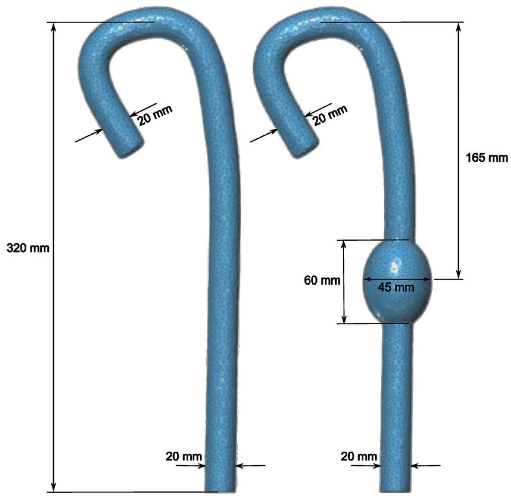
Figure 1. 3D models of the healthy aorta (model #1, left) and the diseased one with an abdominal aneurysm (model #2, right).
Fluids 11 00177 g001
Figure 2. Diagram of the pulsatile circulating system. Q: flow. P1 and P2: site to measure inlet and outlet pressure (P). V1 and V2: unidirectional valves. WK: windkessel chamber. R0, R1 and R2: shut-off valves.
Fluids 11 00177 g002
Figure 3. Methods to estimate the transit time (TT) between two flow rate curves (blue: proximal, red: distal). TTfoot and TTM: time-to-foot and time-to-median transit times. Flow rate curves were normalized to the maximum value (M) only for the TTM method.
Fluids 11 00177 g003
Figure 4. Average velocities (top) and streamlines (bottom) calculated using 4D-Flow acquisitions for the healthy aorta (model #1, left) and the diseased one with an abdominal aneurysm (model #2, right).
Fluids 11 00177 g004
Figure 5. 1D simulation measurements of the healthy aorta (model #1, left) and the aorta with an abdominal aneurysm (model #2, right). Flow rate curves are shown in the first row for different planes orthogonal to the vessel centerline. The linear regression between transit time (TT) and distance are shown in the second and third rows using the median and time-to-foot methods, respectively. PWV was estimated as the inverse of the regression slope.
Fluids 11 00177 g005
Figure 6. 4D-Flow measurements of the healthy aorta (model #1, left) and the aorta with an abdominal aneurysm (model #2, right). Flow rate curves are shown in the first row for different planes orthogonal to the vessel centerline. The linear regression between transit time (TT) and distance are shown in the second and third rows using the median and time-to-foot methods, respectively. PWV was estimated as the inverse of the regression slope.
Fluids 11 00177 g006
Figure 7. 2D-Flow measurements of the healthy aorta (model #1, left) and the aorta with an abdominal aneurysm (model #2, right). Flow rate curves are shown in the first row for different planes orthogonal to the vessel centerline. The linear regression between transit time (TT) and distance are shown in the second and third rows using the median and time-to-foot methods, respectively. PWV was estimated as the inverse of the regression slope.
Fluids 11 00177 g007
Figure 8. Flowmeter lab measurements of the healthy aorta (model #1, left) and the aorta with an abdominal aneurysm (model #2, right). Flow rate curves are shown in the first row for different planes orthogonal to the vessel centerline. The linear regression between transit time (TT) and distance are shown in the second and third rows using the median and time-to-foot methods, respectively. PWV was estimated as the inverse of the regression slope.
Fluids 11 00177 g008
Figure 9. Comparison of PWV values obtained in model #1 (healthy aorta) and model #2 (abdominal aneurysm) with the transit time median (TTM) and time-to-foot (TTfoot) methods for all measurements. The theoretical PWV value calculated for the healthy aorta using the Moens–Korteweg equation (M-K) is shown with a dashed line.
Fluids 11 00177 g009
Disclaimer/Publisher’s Note: The statements, opinions and data contained in all publications are solely those of the individual author(s) and contributor(s) and not of MDPI and/or the editor(s). MDPI and/or the editor(s) disclaim responsibility for any injury to people or property resulting from any ideas, methods, instructions or products referred to in the content.