Error Estimation for Adaptive Mesh Refinement in Droplet Simulations

Abstract

We present a one-dimensional shear-force-driven droplet formation model with a flux-based error estimator. The model is derived using asymptotic expansion and a front-tracking method to simulate the droplet interface. The model is then discretized using the Galerkin finite element method in the mixed form. However, the solution gradients exhibit large jumps across element boundaries and can grow rapidly due to the highly convective pinch-off process. This leads to an erroneous droplet interface and incorrect curvature. Therefore, the mesh must be sufficiently refined to capture the interface accurately. The mixed form of the governing equation naturally provides smooth interface gradients that can be used to compute the error estimate. The computed error estimate is then used to drive the adaptive mesh refinement algorithm. The efficacy of the error estimator is illustrated by comparing the droplet profiles obtained with adaptive refinement to those obtained with regular refinement. The adaptive mesh refinement approach reduces the computational cost significantly without compromising accuracy. For an 85% glycerol droplet in co-flowing air, AMR reproduces pinch-off location, surface area, volume, and pinch-off time with only ≈1% accuracy loss compared to the highly refined reference while reducing wall-clock time from 638 s to 153 s (4.17× speedup) and reducing the maximum element count from 800 to 146 (81.75% reduction).

1. Introduction

The formation of droplets and bubbles is a mature field in physics. These surface-tension-driven phenomena have been deeply explored using interface-tracking and interface-capturing approaches. Historically, the accurate description of free surface flows emerged after Laplace [1] and Young [2] explained the role of mean curvature and the surface tension force as a source of instability in 1805. Eggers and Villermaux presented a comprehensive review of the liquid break-up process [3]. Starting with the initial fluid column, the drop becomes heavier by continuously adding fluid. Under an external force like gravity, the instabilities start to grow on the interface. Meanwhile, the surface tension minimizes the surface energy by decreasing the radius of the fluid column. A spherical droplet starts to form at the end of the fluid column hanging from a very thin neck. Eventually, the radius becomes zero and a droplet separates from the initial fluid column. The point of zero radius is called the “pinch-off" point. After the primary pinch-off, the neck recoils due to the unbalanced surface tension. The capillary waves due to this recoil perturb the interface before the tip can collapse back to the top of the fluid cone. This leads to a secondary breakup creating smaller droplets, which are called “satellite drops”.

Inaugural work on the computational modeling of droplet formation was done by Eggers and Dupont [4]. Their work involved finite difference formulation of the one-dimensional asymptotic model. Ambravaneswaran et al. [5] explored a finite element version of the same model. This model was only explored with the gravitational force as an external force. However, many industrial applications such as atomization and droplet entrainment in annular flow [6,7] and microfluidic devices [8,9,10] involve droplet formation in a shear-force-driven environment. Using the same asymptotic approach for shear-induced droplets, we considered a one-dimensional model that estimates droplet sizes for an environment with co-flowing fluids [11]. For applications with a symmetrical structure of droplet formation, this one-dimensional model with the interface tracking approach is advantageous in terms of computational costs, while still maintaining the accuracy required for comparison with experiments. Nonetheless, this shear-induced droplet model deals with a wide range of external force magnitudes that induce a wide range of interface instability timescales.

The instability leading to the pinch-off point requires a finer mesh in the region of high curvature. As the interface evolves with the progression of numerical simulation, the mesh must be refined to control discretization errors, especially in the singularity regions. Because this range of timescales makes the location and rate of mesh refinement difficult to predict a priori, an adaptive strategy driven by a reliable error estimator is needed. However, the work on an error estimator for the one-dimensional droplet formation model is not fully explored yet. The field of a posteriori error estimation has been under continuous and rigorous improvement since the 1980s [12]. Babuška and Rheinboldt [13,14] established foundational residual-based reliability ideas, while Kelly et al. [15] developed practical flux-jump indicators for engineering finite element workflows. Ainsworth and Oden [16] presented rigorous reliability and efficiency theory, explicitly discussing the unknown multiplicative constants that arise in classical residual-type bounds. Dörfler [17] showed that bulk marking yields provable contraction of the estimator in adaptive cycles. A recent synthesis of modern methods is given in [18]. In contrast to classical post-processed recovery estimators, the present mixed formulation provides a smooth slope variable directly as part of the coupled solve, therefore naturally providing us with a robust error estimator as a part of the solution. In the present work, we combine the mixed formulation with the traditional error estimation approach to address the research gap and show that the mixed finite element formulation of our one-dimensional model naturally provides an effective error estimator for adaptive mesh refinement.

In the following sections, we describe the one-dimensional droplet pinch-off model and explain the need for an error estimator. Then, we explore the flux-based error estimation approach and show that the mixed form naturally provides a smooth flux to compute error bounds. Finally, we illustrate the effectiveness of our error estimator using adaptive mesh refinement.

2. Problem Description

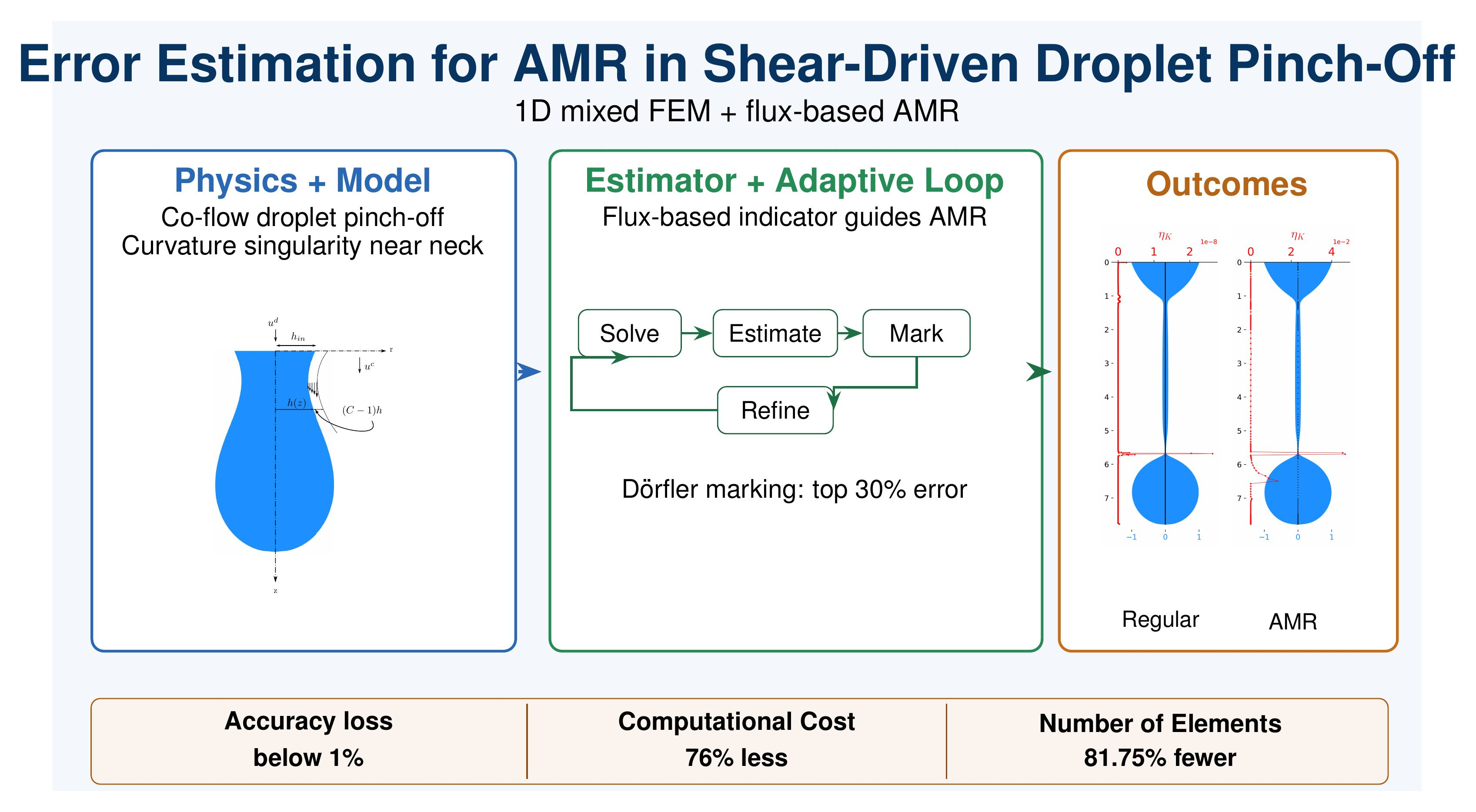
We consider a fluid column slowly flowing with a constant velocity $u^d$ out of a nozzle with radius $h_{in}$. The continuous (or outer) fluid is co-flowing with the dispersed (or inner) fluid column but with a higher velocity $u^c$ in a capillary tube with radius R. Figure 1 shows a schematic of this co-flowing fluid scenario. The superscripts d and c represent dispersed phase and continuous phase fluids, respectively.

For the suspended fluid column without a background fluid, we start with the Navier–Stokes equations in cylindrical coordinates. The pinch-off process happens in finite time due to the surface tension forces trying to minimize the surface energy by contracting the interface in the radial direction. The radial contraction is faster than the axial elongation, which allows us to expand the solution variables asymptotically in r. Finally, the normal forces are balanced by the surface tension forces, which simplifies the equations to a one-dimensional model.

Similarly, we consider the droplet pinch-off of the fluid column in another co-flowing fluid under the gravitational and shear forces. We consider co-flowing fluids with symmetry preserved in the angular direction. This provides the basis for the one-dimensional approach. The continuous fluid affects the droplet morphology by applying shear forces on the interface between the two fluids. This shear-force effect can be approximated using an asymptotically derived force balance on the interface, yielding the one-dimensional governing equations [11]. The full derivation can be found in [19].

This one-dimensional shear-driven model and its mixed finite-element discretization have been previously validated against experiments and high-fidelity computations in our earlier works [11,20]. In this manuscript, we focus on how the estimator provided by the mixed formulation can be used to drive efficient adaptive refinement.

The momentum and the interface equations are given as follows.

$$\begin{array}{c}\hfill {\displaystyle \frac{\partial u^d}{\partial t}}+u^d{\displaystyle \frac{\partial u^d}{\partial z}}+{\displaystyle \frac{\gamma }{\rho }}{\displaystyle \frac{\partial \mathcal{K}}{\partial z}}-{\displaystyle \frac{6{\nu }^d}{h}}{\displaystyle \frac{\partial u^d}{\partial z}}{\displaystyle \frac{\partial h}{\partial z}}\left(1+{\displaystyle \frac{{\mu }^c}{{\mu }^d}}\right)-3{\nu }^d{\displaystyle \frac{{\partial }^2{u}^d}{\partial z^2}}\left(1+{\displaystyle \frac{2}{3}}{\displaystyle \frac{{\mu }^c}{{\mu }^d}}\right)\end{array}$$

$$\begin{array}{c}\hfill +{\displaystyle \frac{2}{{\rho }^d}}{\displaystyle \frac{d{p}^c}{dz}}+{\displaystyle \frac{1}{2{\rho }^{d}ln\left(C\right)}}{\displaystyle \frac{d{p}^c}{dz}}-\left(1-{\displaystyle \frac{{\rho }^c}{{\rho }^d}}\right)g=0\end{array}$$

(1)

$$\begin{array}{c}\hfill {\displaystyle \frac{\partial h}{\partial t}}+u^d{\displaystyle \frac{\partial h}{\partial z}}+{\displaystyle \frac{h}{2}}{\displaystyle \frac{\partial u^d}{\partial z}}=0\end{array}$$

(2)

Here, the parameters $\gamma$, $\rho$, $\nu$, $\mu$, and p represent the surface tension coefficient, density, kinematic viscosity, dynamic viscosity, and pressure, respectively. The superscript represents dispersed or continuous phase fluid. $\mathcal{K}$ is the curvature defined by

$$\begin{array}{c}\hfill \mathcal{K}=\left[{\displaystyle \frac{1}{h{\left(1+{\left(\frac{\partial h}{\partial z}\right)}^2\right)}^{1/2}}}-{\displaystyle \frac{\frac{{\partial }^{2}h}{\partial z^2}}{{\left(1+{\left(\frac{\partial h}{\partial z}\right)}^2\right)}^{3/2}}}\right]\end{array}$$

(3)

The quantity $(C-1)h$ defines the thickness of the shear layer in the continuous phase flow, which defines how much force is experienced by the dispersed phase droplet. The parameter C is a free parameter that can be defined using curve-fitted monotonic functions on the numerical and experimental data. In [11], it was shown that this single parameter model can account for behavior in a wide range of dimensionless parameter values.

The system of governing equations given by Equations (1) and (2) is then discretized using a Galerkin finite element method in the mixed form [11]. We will use finite element spaces $\mathcal{U}$ for velocity, $\mathcal{H}$ for radius, and $\mathcal{S}$ for the slope variable, an auxiliary variable introduced in the mixed formulation to approximate the interface slope $\partial h/\partial z$. Now we can express the mixed finite element weak form as

$$\begin{array}{c}\hfill {\int }_{\mathsf{\Omega }}q\left[{\displaystyle \frac{\partial u}{\partial t}}+u{\displaystyle \frac{\partial u}{\partial z}}-{\displaystyle \frac{6\nu }{h}}{\displaystyle \frac{\partial h}{\partial z}}{\displaystyle \frac{\partial u}{\partial z}}\left(1+{\displaystyle \frac{{\mu }^c}{{\mu }^d}}\right)+{\displaystyle \frac{\gamma }{\rho }}\left\{-{\displaystyle \frac{s\frac{\partial s}{\partial z}}{h{\left(1+s^2\right)}^{3/2}}}-{\displaystyle \frac{s}{h^2{\left(1+s^2\right)}^{1/2}}}\right\}\right.\\ \hfill \left.+{\displaystyle \frac{2}{{\rho }^d}}{\displaystyle \frac{d{p}^c}{dz}}+{\displaystyle \frac{1}{2{\rho }^{d}ln\left(C\right)}}{\displaystyle \frac{d{p}^c}{dz}}-\left(1-{\displaystyle \frac{{\rho }^c}{{\rho }^d}}\right)g\right]d\mathsf{\Omega }\\ \hfill +{\int }_{\mathsf{\Omega }}\nabla q\left[3\nu \left(1+{\displaystyle \frac{2}{3}}{\displaystyle \frac{{\mu }^c}{{\mu }^d}}\right){\displaystyle \frac{\partial u}{\partial z}}+{\displaystyle \frac{\gamma }{\rho }}{\displaystyle \frac{\frac{\partial s}{\partial z}}{{\left(1+s^2\right)}^{3/2}}}\right]d\mathsf{\Omega }\end{array}$$

$$\begin{array}{c}\hfill -{\int }_{\mathsf{\Gamma }}q\left[3\nu \left(1+{\displaystyle \frac{2}{3}}{\displaystyle \frac{{\mu }^c}{{\mu }^d}}\right){\displaystyle \frac{\partial u}{\partial z}}+{\displaystyle \frac{\gamma }{\rho }}{\displaystyle \frac{\frac{\partial s}{\partial z}}{{\left(1+s^2\right)}^{3/2}}}\right]d\mathsf{\Gamma }=0\end{array}$$

(4)

$$\begin{array}{c}\hfill {\int }_{\mathsf{\Omega }}v\left[{\displaystyle \frac{\partial h}{\partial t}}+u{\displaystyle \frac{\partial h}{\partial z}}+{\displaystyle \frac{h}{2}}{\displaystyle \frac{\partial u}{\partial z}}\right]d\mathsf{\Omega }=0\end{array}$$

(5)

$$\begin{array}{c}\hfill {\int }_{\mathsf{\Omega }}w\left[s-{\displaystyle \frac{\partial h}{\partial z}}\right]d\mathsf{\Omega }=0\end{array}$$

(6)

where $u,q\in \mathcal{U}$, $h,v\in \mathcal{H}$, and $s,w\in \mathcal{S}$. Equations (4)–(6) are solved using the continuous Galerkin method with $C^0\left(\mathsf{\Omega }\right)$ elements. The curvature now depends on the slope variable s instead of $\partial h/\partial z$, as shown below. This is a key point that allows us to use the mixed formulation to compute the error estimate, as will be explained in the next section.

$$\begin{array}{c}\hfill \mathcal{K}=\left[{\displaystyle \frac{1}{h{\left(1+s^2\right)}^{1/2}}}-{\displaystyle \frac{\frac{\partial s}{\partial z}}{{\left(1+s^2\right)}^{3/2}}}\right]\end{array}$$

(7)

The solution algorithm involves a moving mesh and calculates the droplet length in a self-consistent way. The algorithm is explained in [20], and has been implemented using the PETSc libraries [21,22].

The flow becomes highly convective as the droplet interface evolves up to the point at which the neck begins to form. The radial contraction of the interface accelerates faster than the axial elongation, rapidly approaching the singularity. This behavior must be captured accurately to obtain precise equilibrium droplet profiles. In addition, the interface is advected with the flow, so that errors in the interface location at one step strongly affect later steps in the flow.

3. Error Estimation

When approaching the singularity, the high-curvature regions quickly develop high stresses. An error in the solution can cause the interface to advect in an incorrect direction, yielding an incorrect droplet profile. A coarser mesh must be refined to improve the solution in those regions and obtain an accurate force balance, leading to more accurate droplet profiles. This refinement can be done adaptively by estimating the true error in the solution using a posteriori error estimation approach. The foremost goal is to compute the discretization error in the droplet interface evolution.

Since the solution is approximated with $C^0\left(\mathsf{\Omega }\right)$ continuity, the solution gradients are discontinuous across the element boundaries. This discontinuity significantly impacts the curvature computation and can produce erroneous equilibrium droplet profiles. We use a flux-recovery-based approach to drive the adaptive mesh refinement. The flux-recovery approach aims to post-process a smooth gradient from the finite element solution and construct the error estimator from the difference between the smoothed and non-smoothed gradients.

In the droplet pinch-off model, the solution consists of the velocity (u) and the droplet radius (h). The mixed formulation additionally includes an approximation of the gradient $\partial h/\partial z$ as part of the solution, which is denoted by s. In other words, the mixed variable s already provides a smooth gradient of h. If the true gradient is $\partial \overline{h}/\partial z$, the quantity s is assumed to retain better accuracy than $\partial h/\partial z$ since the slope (or flux) s is part of the equilibrium equations and coupled with the curvature derivatives in the momentum equations. The true error norm in the gradient can be written as

$$\begin{array}{cc}\hfill \left|\left|e\right|\right|& =\left|\left|{\displaystyle \frac{\partial \overline{h}}{\partial z}}-{\displaystyle \frac{\partial h}{\partial z}}\right|\right|\approx \left|\left|s-{\displaystyle \frac{\partial h}{\partial z}}\right|\right|\hfill \end{array}$$

(8)

The quality of the estimate clearly depends on how good the approximation s is of the true slope $\partial \overline{h}/\partial z$. Assuming there exists $c\in (0,1)$ such that

$$\begin{array}{c}\hfill \left|\left|{\displaystyle \frac{\partial \overline{h}}{\partial z}}-s\right|\right|\le c\left|\left|{\displaystyle \frac{\partial \overline{h}}{\partial z}}-{\displaystyle \frac{\partial h}{\partial z}}\right|\right|\end{array}$$

(9)

A natural choice is to define c as the relative defect

$$\begin{array}{c}\hfill c:={\displaystyle \frac{\left|\left|\frac{\partial \overline{h}}{\partial z}-s\right|\right|}{\left|\left|\frac{\partial \overline{h}}{\partial z}-\frac{\partial h}{\partial z}\right|\right|}}\end{array}$$

when the denominator is nonzero (and $c=0$ otherwise). By non-negativity of norms, $c\ge 0$. The mixed formulation provides s through an additional equilibrium relation and direct coupling to curvature terms in the momentum balance, so s is taken as at least as informative as the raw primal gradient. Under this approximation property,

$$\begin{array}{c}\hfill \left|\left|{\displaystyle \frac{\partial \overline{h}}{\partial z}}-s\right|\right|\le \left|\left|{\displaystyle \frac{\partial \overline{h}}{\partial z}}-{\displaystyle \frac{\partial h}{\partial z}}\right|\right|\end{array}$$

which implies $0\le c\le 1$, and strict improvement gives $c<1$. Using the triangle inequality, the bounds on the true error in terms of the error estimator follow directly:

$$\begin{array}{c}\hfill {\displaystyle \frac{\eta }{1+c}}\le \left|\left|e\right|\right|\le {\displaystyle \frac{\eta }{1-c}}\end{array}$$

(10)

where $\eta =\left|\left|s-\partial h/\partial z\right|\right|$ is the error estimate of the true error. It is clear that the smaller the c, the better the error estimate. Thus, c is an estimator-quality factor: values near 0 yield tight bounds, while values near 1 yield loose but still valid bounds.

The traditional a posteriori error estimation methods, such as residual-based and flux-based methods, use the residual in each element and the flux jumps across the elemental interfaces. However, these error bounds include an unknown multiplicative constant. Our approach can also be viewed from the residual-based error estimation perspective. A residual-based a posteriori error estimation approach directly utilizes the finite element solution. Defining the error in the energy norm, one can also derive upper and lower error bounds for the error in the slope s using the element residuals of Equation (6).

Here, the error bounds given in Equation (8) are used to refine the mesh adaptively. A simple h-refinement can be done cyclically:

solve → estimate error → mark elements → refine

We use two strategies to refine the mesh and compare their effectiveness.

(1)

The regular refinement, where elements are doubled at each refinement cycle.

(2)

The elements are marked using Dörfler’s method [17], where the elements are marked such that the total error in the marked elements is $\lambda$ times the total error in the entire domain.

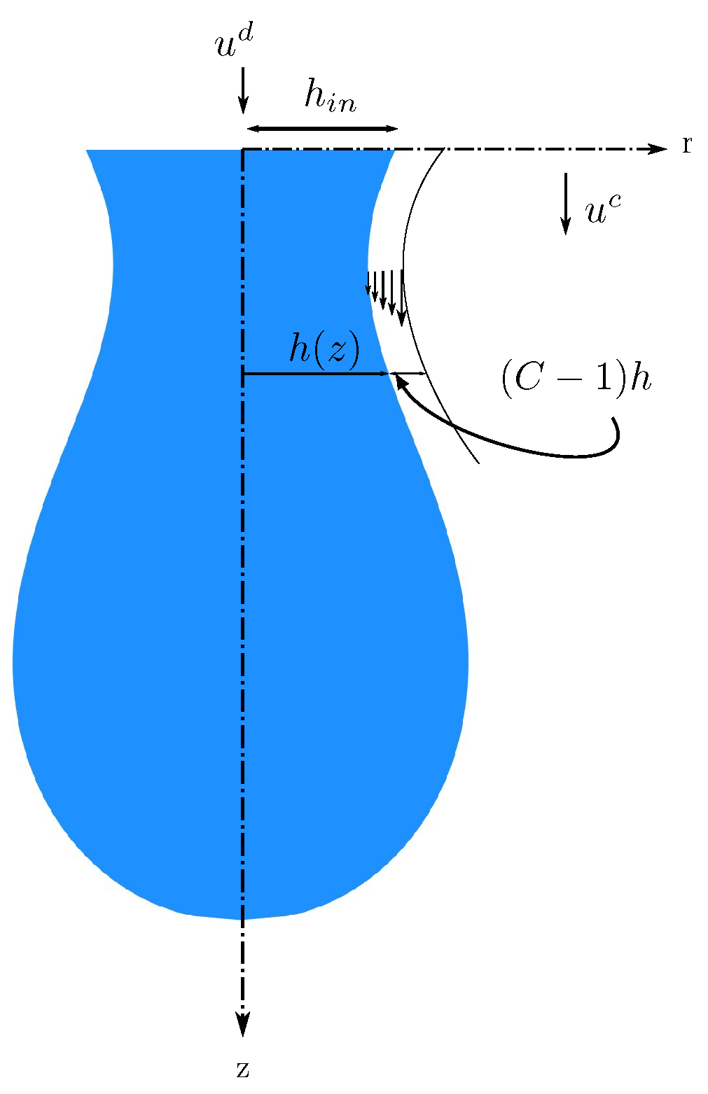
Initially the finite element system is solved using PETSc TSSolve. The pointwise error is then computed and the elements are marked using Dörfler’s criterion. The mesh is refined, and the solution is projected onto the new mesh. This process is repeated until the pinch-off condition is satisfied. Figure 2 shows a flowchart of this solution algorithm. All simulations were run in serial on the 13th Gen Intel(R) Core(TM) i9-13980HX. The code uses PETSc v3.23.0 and was compiled with gcc 13.

4. Results

The droplet simulations presented in this section are for an 85% glycerol solution with an inlet velocity of 5 mm/s and a co-flowing air stream at 1 m/s. The nozzle inlet radius is 2.5 mm and the outer capillary tube radius is 25 mm. The material properties are taken from [20].

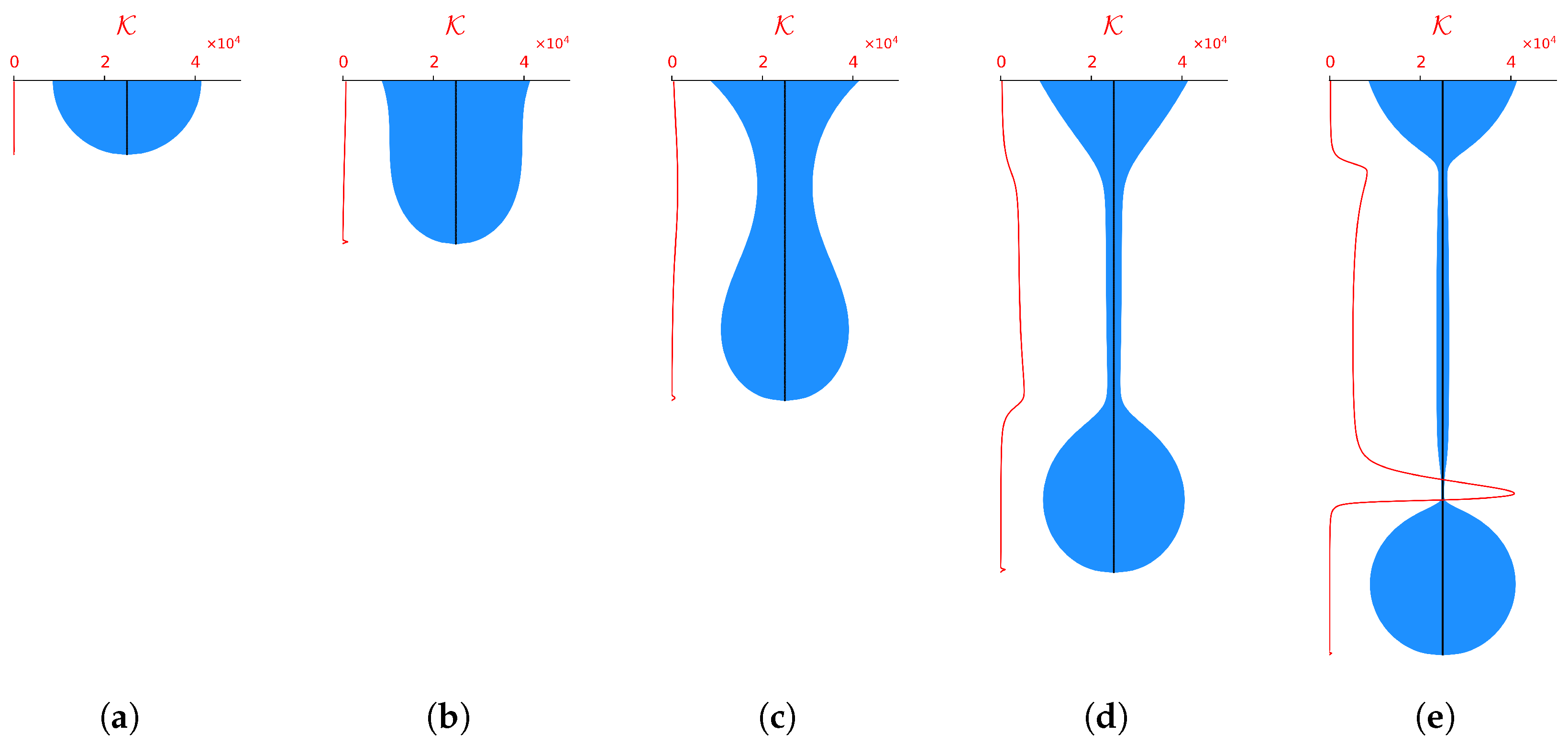
The error estimation approach is motivated entirely by the need to capture regions with sharp changes in the mean curvature. Therefore, it is important to understand how the mean curvature evolves in order to contextualize the error estimates. Figure 3 shows a sequence of images illustrating the evolution of mean curvature as the droplet evolves up to the primary pinch-off. The mean curvature is computed using the finite element solution and plotted along the droplet length. The initial mesh is uniform with 50 elements. As the droplet length increases, the mesh is regularly refined by doubling the number of elements as the length increases by a factor of 2 to maintain the accuracy of the solution. The droplet evolves roughly up to 8 times the initial length before the primary pinch-off. Therefore, the mesh is refined up to 800 elements, with 4 levels of refinements. The refinement cycle is defined by the non-dimensionalized droplet length $L/h_{in}$, where L is the droplet length and $h_{in}$ is the inlet radius. We refine the mesh when $L/h_{in}>N$, where $N=\{2,4,6\}$ for the first, second, and third refinement cycles. The last refinement cycle is triggered when $h_{min}<{\displaystyle \frac{h_{in}}{50}}$, where $h_{min}$ is the minimum droplet radius. This ensures that the mesh is sufficiently refined to capture the pinch-off process. The pinch-off is concluded when $h_{min}<{\displaystyle \frac{h_{in}}{100}}$.

Because the estimator is available at each step, refinement triggering can in principle be made directly error-driven (e.g., by checking a global threshold on $\eta$) rather than based only on geometric indicators. In this manuscript, we retain the existing stage-based trigger because the unrefined simulations show that the error accumulates as the droplet elongates and curvature variations build up near the neck and pinch-off regions. The length-based condition is therefore used as a practical scheduling device to avoid refining too aggressively at very early stages and to save computational time by refining in bulk only after sufficient interface evolution has occurred. The actual refinement remains estimator-driven: once a refinement stage is activated, the local indicator ${\eta }_K$ is used for marking and localization.

Initially, the mean curvature is largest at the droplet tip. The mean curvature starts increasing in the neck region of the fluid column as the droplet evolves. This is naturally due to the radial shrinkage of the column. Finally, the mean curvature is highest at the pinch-off location when the primary droplet separates from the fluid column. The regions with sharp curvature changes are the top of the neck, the region near the pinch-off, and the droplet tip. Therefore, a higher error is expected in these regions. One notable observation is that the curvature has a kink at the tip of the droplet. This is due to the choice of initial value of $s=-10$ at the tip and kept bounded with a large negative value. However, the solution is invariant to the choice of this initial value as long as it is sufficiently negative. Theoretically, the slope at the tip should be negative infinity. The choice of a large negative value is a practical way to approximate this behavior and to keep the simulation stable.

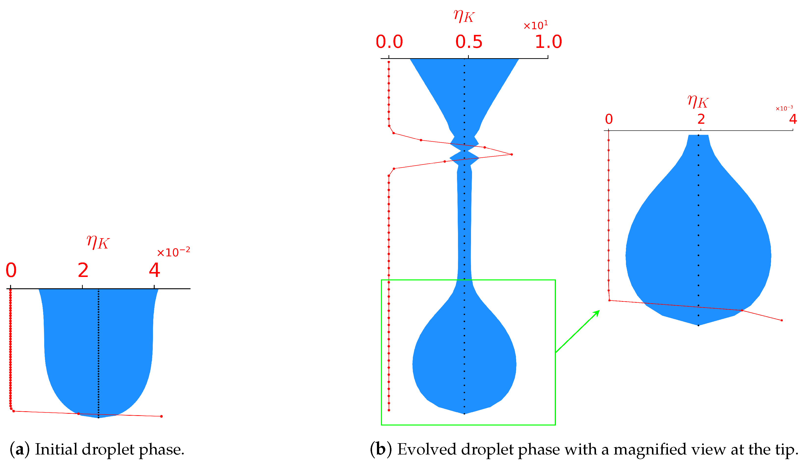
We first report the element-wise errors without performing adaptive mesh refinement. The droplet length and radius are non-dimensionalized using the inlet radius $h_{in}$ in all plots. The element-wise estimated error, denoted by ${\eta }_K$, is shown in Figure 4. The error is plotted for the initial droplet profile and an evolved droplet profile as shown in Figure 4a and Figure 4b, respectively. The initial droplet profile has the highest curvature gradient near the tip. Thus, the highest error is detected at the tip, as shown in the figure.

On the other hand, the evolved droplet has a large error at the top of the neck region. This error is associated with an inaccurate interface representation in the neck region. This inaccuracy leads to a divergence of residuals and simulation failure before reaching the primary pinch-off. The magnified image shows the error magnitude at the tip, which is larger for the last few elements. This suggests that mesh refinement is required to accurately capture the smooth spherical shape at the droplet tip.

Based on the reported errors, the adaptive mesh refinement strategy described in the previous section is applied. As the simulation progresses, we track the error evolution along with the droplet interface. This provides insight into how the error evolves as the curvature changes. Using Dörfler’s strategy, adaptive mesh refinement is performed when the droplet length is greater than N times the inlet radius, where $N=\{2,4,6,\dots \}$. Similar to the regular refinement strategy, the final refinement is performed when $h_{min}<{\displaystyle \frac{h_{in}}{50}}$.

To examine sensitivity to the bulk-marking fraction, we performed a parameter sweep with cumulative-error fractions of 10%, 20%, 30%, 40%, and 50%.

Table 1. Sensitivity of AMR results to Dörfler cumulative-error fraction (monitor-off timings).

Error Fraction	Pinch-Off Loc.	Surface Area	Volume	Pinch-Off Time (s)	Wall Clock (s)
10%	0.7300	$7.5865\times {10}^{-5}$	$6.1931\times {10}^{-8}$	0.5873	107
20%	0.7255	$7.5896\times {10}^{-5}$	$6.1951\times {10}^{-8}$	0.5851	135
30%	0.7186	$7.5964\times {10}^{-5}$	$6.2043\times {10}^{-8}$	0.5845	153
40%	0.7128	$7.5869\times {10}^{-5}$	$6.1894\times {10}^{-8}$	0.5829	182
50%	0.7200	$7.5795\times {10}^{-5}$	$6.1846\times {10}^{-8}$	0.5820	212

shows the expected trade-off: lower fractions (10–20%) are faster but produce larger deviations in pinch-off location, while higher fractions (40–50%) increase cost substantially without a commensurate improvement across all quantities of interest. The 30% setting provides the best overall balance of accuracy and efficiency for this case and is therefore selected as the sweet-spot value in this study.

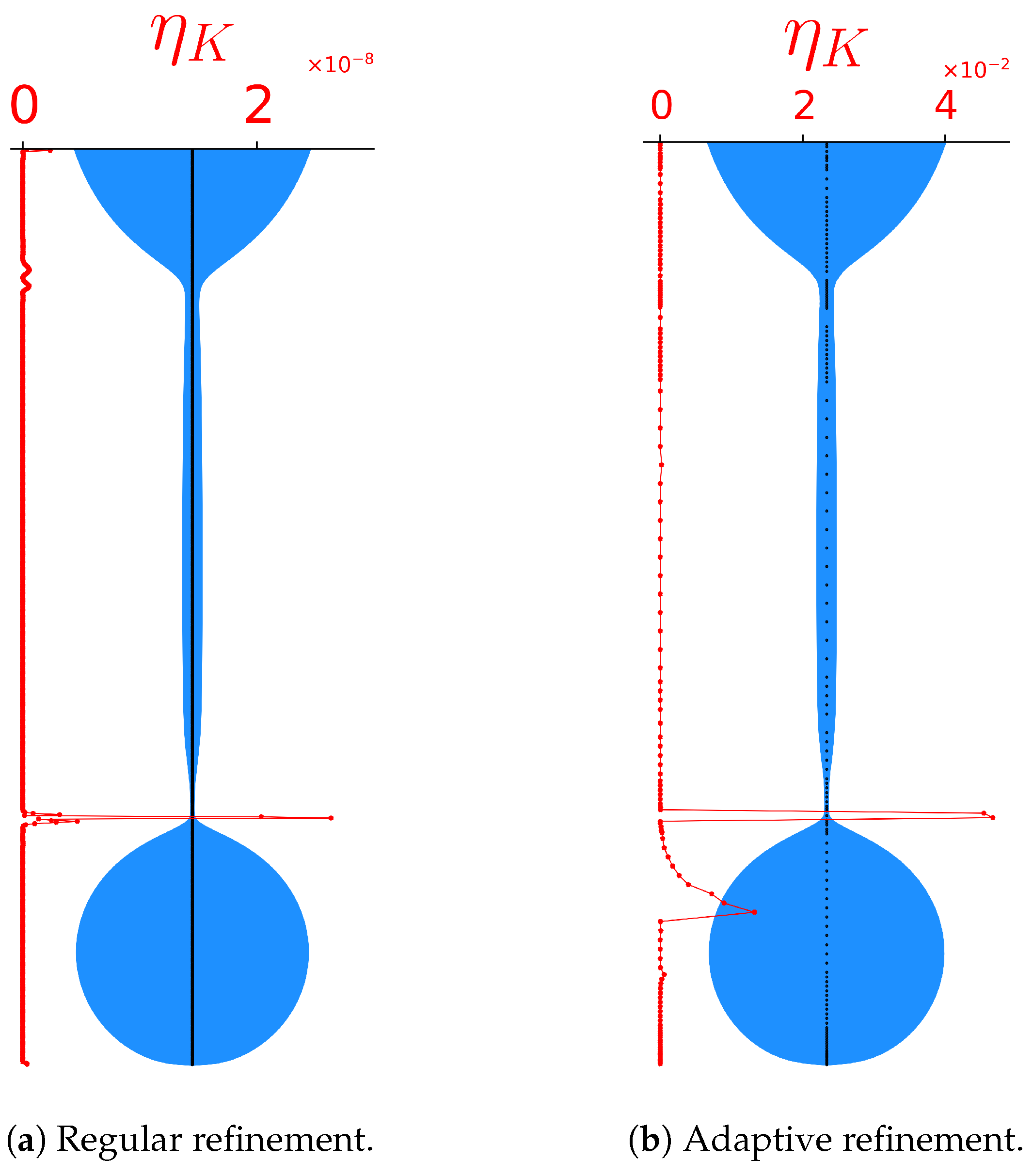
Figure 5 directly compares regular refinement (left) and adaptive refinement using Dörfler marking (right) at the same evolution stage. The regular strategy, shown in Figure 5a, reduces the error by uniformly adding elements over the full domain. As a result, the error in the neck region is significantly reduced. The largest error is at the pinch-off location, where the curvature changes are highest. Additionally, the error at the top of the neck and at the tip is also apparent. Nonetheless, the error is reduced to the order of ${10}^{-8}$, which is sufficient to capture the droplet profile accurately. We use this as a reference to compare the Dörfler marking approach, which refines only the elements with the largest error.

Figure 5b shows the error distribution for the Dörfler marking approach. Similar to the regular refinement, the error is largest at the pinch-off location. The error is reduced to the order of ${10}^{-2}$, which is smaller than the unrefined case but larger than the regular refinement case. However, the droplet profile is significantly improved compared to the unrefined case, and the instabilities are removed. Moreover, the pinch-off droplet profile is visually indistinguishable from the regular refinement case, indicating that the error level is sufficient to capture the droplet profile accurately. The node markers in Figure 5b show visible clustering near the neck and pinch-off region, confirming that refinement is spatially localized in the regions identified by large estimator values.

The difference between error levels of order ${10}^{-8}$ (regular refinement) and ${10}^{-2}$ (adaptive case) should be interpreted in a goal-oriented sense: the AMR solution is sufficiently accurate for the reported quantities of interest and interface shape, even though its global estimator norm is larger. Uniform refinement aggressively reduces error in low-impact regions, whereas Dörfler marking concentrates effort in dynamically dominant regions controlling pinch-off morphology.

Another crucial note is that the purpose of the present estimator is to target the spatial discretization error. To keep temporal error low, we start with $\mathsf{\Delta }t={10}^{-4}$ and reduce the time step by half at every spatial refinement level. We also checked the quantities of interest using constant time steps $\mathsf{\Delta }t={10}^{-5}$ and $\mathsf{\Delta }t={10}^{-6}$ and observed no change; therefore, we use the refinement-coupled time-step strategy in this work.

Comparing Figure 5a,b, both approaches recover a smooth interface and remove the visible instability near the neck. However, a quantitative comparison is also necessary to fully assess the performance of the Dörfler marking approach.

Table 2. Comparison of regular refinement and AMR for pinch-off metrics and computational cost. Relative differences are computed with respect to the regular-refinement result.

Quantity	Regular Refinement	AMR	Relative Difference
Non-dimensional pinch-off location	0.7200	0.7186	0.1944%
Pinch-off droplet surface area	$7.5548\times {10}^{-5}$	$7.5964\times {10}^{-5}$	0.5506%
Pinch-off volume	$6.1558\times {10}^{-8}$	$6.2043\times {10}^{-8}$	0.7878%
Pinch-off time (s)	0.5769	0.5845	1.3174%
Wall-clock time (s)	638	153	76.02% reduction
Maximum number of elements	800	146	81.75% reduction
Global error	$7.59\times {10}^{-8}$	$1.33\times {10}^{-1}$	–

compares the key quantities of interest and simulation time for a representative regular-refinement run and an AMR run. The quantities are pinch-off location, surface area, volume, and pinch-off time. The AMR case reproduces all quantities with sub $1\%$ inaccuracy compared to the regular-refinement reference, except the pinch-off time, which has $1.3174\%$ difference. This is achieved while reducing wall-clock time from 638 s to 153 s, which is a $76\%$ reduction in computational cost. In other words, this AMR provides a speedup of $4.17\times$, while maintaining close agreement in all quantities of interest. This comparison is evidence of the effectiveness of the error estimator in driving the adaptive mesh refinement to capture the droplet profile accurately while significantly reducing computational cost.

The key point is that AMR achieves nearly the same quantities of interest while using far fewer elements. The regular-refinement case reaches 800 elements, whereas the AMR case uses at most 146 elements. This large reduction in mesh size is the main reason for the substantial savings in computational cost.

Validation

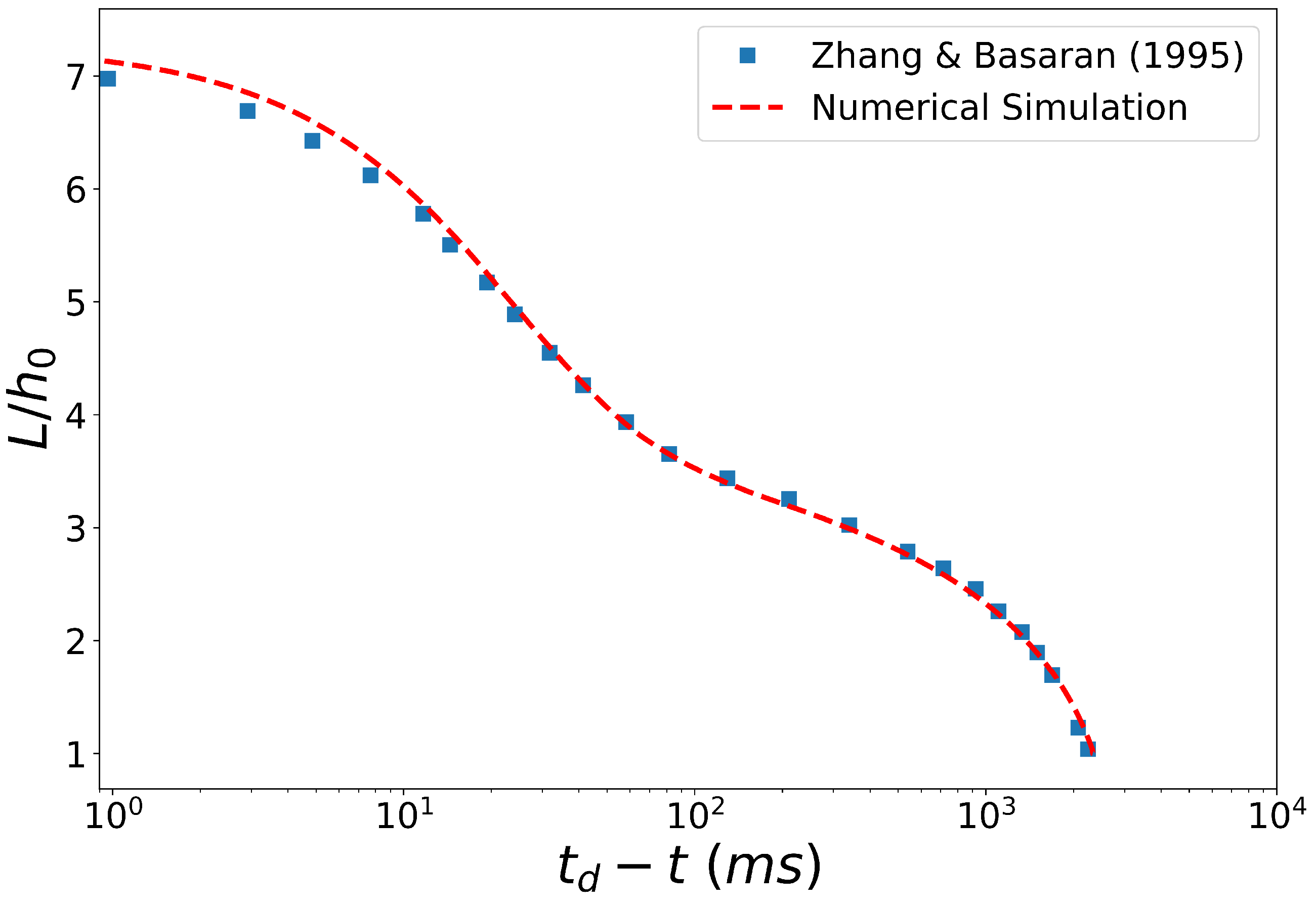
The error estimator is robust and shows an impressive improvement compared to the regular refinement case. However, it is crucial to perform validation through comparison with experimental data. Zhang and Basaran [23] performed experiments on the pinch-off of 85% glycerol droplets and reported the morphological evolution of the droplet interface. We compare the non-dimensional droplet length evolution between the AMR simulation and the experimental data in Figure 6. The AMR simulation shows good agreement with the experimental data, capturing the droplet elongation and pinch-off dynamics accurately. The slight discrepancies observed can be attributed to experimental uncertainties and added streamline upwinding in the numerical model. Overall, the validation confirms that the proposed error estimator and adaptive mesh refinement strategy are effective in accurately simulating droplet pinch-off phenomena.

Although the numerical examples in this work are presented for a single fluid-property set, the estimator itself is not constructed from material-dependent coefficients. It is based on the discrepancy between the mixed-variable slope and the recovered interface slope, and is therefore applicable in the same form to other droplet cases. However, the pinch-off dynamics do depend on the material properties and operating conditions because these affect the rate of elongation, the onset of necking, and the localization of high-curvature regions. Consequently, the AMR control parameters built around the estimator, such as the trigger stage, marking fraction, and refinement schedule, may need to be tuned for a given case to obtain the best balance between accuracy and computational cost. Extending the study to additional fluid-property and operating-condition combinations is therefore a natural direction for future work.

The one-dimensional model has been previously used for uncertainty quantification (UQ) analysis of droplet atomization in hybrid rocket combustion [24]. The error estimator can be used to drive the adaptive mesh refinement in the UQ simulations, allowing for more accurate and efficient exploration of the parameter space. This is particularly important in UQ analyses, where a large number of simulations are required to capture the variability in the system. By using the error estimator to refine the mesh adaptively, we can ensure that each simulation is performed with sufficient accuracy while minimizing computational costs.

5. Conclusions

We presented a simple yet effective strategy to compute the error estimate for droplet simulations with a front-tracking method. The one-dimensional model used for the simulations is accurate for shear-induced droplets in a co-flowing environment. The mixed form equations naturally incorporate a smooth flux as part of the solution, enabling flux-based error estimation. The comparison of error evolution for 85% glycerol droplets in co-flowing air is presented for unrefined, regularly refined, and adaptively refined grids. This comparison shows that the adaptively refined grid provides improved stability and accuracy in capturing the droplet interface. The AMR approach keeps the quantities of interest within $1\%$ of the regular-refinement case while reducing the computational cost by ≈76% by using ≈82% fewer elements.