Experimental and Mathematical Modeling of Unsteady Flow Around Darrieus H-Rotor of Vertical-Axis Wind Turbines

Abstract

Small-scale vertical-axis wind turbines (VAWTs) are increasingly essential for the “blue economy,” providing autonomous power to remote coastal communities, offshore platforms, and marine industries. However, the design of efficient Darrieus-type rotors is complicated by complex unsteady aerodynamics, particularly the phenomenon of dynamic stall. This study aims to establish and validate a cost-effective yet accurate mathematical modeling approach for simulating unsteady turbulent flow around a Darrieus H-rotor to support practical engineering applications. The research methodology integrates computational fluid dynamics (CFD) with physical experiments in a hydrodynamic channel. The numerical model utilizes the unsteady Reynolds-averaged Navier–Stokes (URANS) equations closed with the Strain-Adaptive Linear Spalart–Allmaras (SALSA) turbulence model, chosen for its efficiency in capturing flow separation. The system of initial equations was being devised relatively to an arbitrary curvilinear coordinate system. The pressure and velocity fields have been coordinated using the artificial compressibility method adapted to calculate non-stationary problems. Experimental verification was conducted in the GT-400 hydrodynamic tube using a three-bladed H-rotor model, where flow structures were visualized via the colored jet method at tip speed ratios λ ranging from 2 to 5 and Reynolds number 1470. The findings reveal that dynamic stall occurs over a significant portion of the blade trajectory, characterized by vortex generation at the leading edge and subsequent advection along the chord. Qualitative comparison demonstrates a high degree of correlation between the calculated vortex dynamics and physical flow spectra. These results confirm that the URANS-SALSA approach provides a rational compromise between computational cost and physical accuracy.

1. Introduction

Offshore wind power has been around for many years and keeps growing rapidly. The first offshore wind farm was put in operation in Denmark in 1991. In 2020, the number of offshore wind farms according to the World Forum Offshore Wind (WFO) [1,2] reached the number of 162. An analysis by the International Energy Agency (IEA) has shown that offshore wind power can generate 18 times more electricity than the existing need for it today. Offshore wind power is an example demonstrating the benefits of the “blue economy”, which the UNO defines as a set of economic activities associated with oceans, seas and coastal areas [3,4]. The offshore power plants currently commissioned are based on horizontal-axis wind turbines (HAWTs). They are located mainly on stationary foundations, or they look like giant floats in deeper waters. In order to reduce the cost of generated electricity and bring it closer to commercially competitive values, developers increase the power, and, consequently, the size of individual wind turbines. Over the past few years, the unit capacity of such wind turbines has increased from 5 MW to 12 MW [4,5]. A well-known large manufacturer of the Vestas large-scale wind turbines recently has announced the launch of wind turbines featuring up to 15 MW capacity [6]. Undoubtedly, these wind turbines are the basic type of power generating devices, paving the way to provide the world’s grid electricity with clean renewable energy. At the same time, there are a large number of communities that consume relatively small amount of electricity, anyway, being unable to do without it. These include typical objects of the blue economy such as island and remote coastal communities and industries.

The lack of electrical grid infrastructure in remote communities and industries and their dependence on electricity, usually generated by diesel generators, is a problem for providing electricity to the blue economy sectors. Small mobile platforms featuring medium and small wind turbines are required to make renewable energy sources more accessible for such industries.

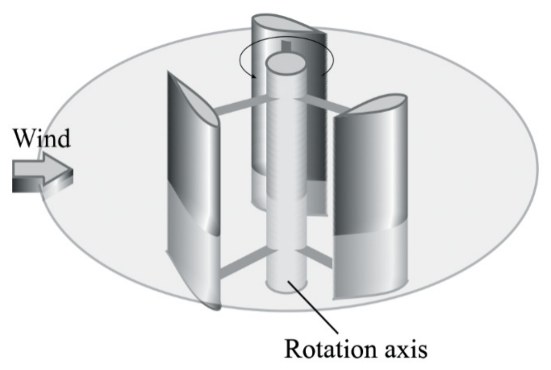
Modular power platforms for astronauts and authorized observers can be created using vertical-axis wind turbines (VAWTs) put on a fixed or floating base. The ability to increase the capacity of individual wind turbines at lower project costs makes it more attractive [7]. Several offshore energy projects are known, based on floating VAWTs with various constructive varieties of the Darrieus rotor, such as classic, H-rotors, helicoidal rotors or their combinations. The Deepwind project [8] uses a turbine with a classic Darrieus rotor with a capacity of 5 MW made in the form of a float fastened with flexible connection to the bottom. Conceptual projects Nenupher Vertiwind and Nenupher Twinfloat provided, in the first case, the use of a VAWT with a Darrieus H-rotor with a capacity of 2 MW, and in the second case, two opposite turbines with a Daria N-Rotor, installed on one floating base with a total capacity of 5 MW [9,10]. SKWID hybrid energy systems developed by MODEC and OceanHydroOmni created by the international group of researchers are intended for the use of wind energy and ocean flows. In their construction, they are supposed to use helicoid and Darrieus H-rotors [11]. British company VertAx Wind Ltd. announced the development of a floating VAWT with a Darrieus H-rotor with a capacity of several megawatts [12]. One of the successfully implemented projects of offshore energy platforms is the Norwegian pilot turbine SeaTwirl S1 with a Darrieus H-rotor and a capacity of 30 kW installed on the coast of Sweden [13]. The installation of SeaTwirl S2 with a capacity of 1 MW, which is the evolution of the S1 turbine, is under development. Mohan Kumar et al. [14] reviewed the evolution of Darrieus VAWTs, from its origins to its current applications, explaining in detail the main types of VAWTs.

As reviewed by Li et al. [15], a large number of scientific articles are devoted to various aspects of scientific research aimed at modeling aerodynamics, hydrodynamics, general mechanics and calculating the design parameters of offshore floating energy platforms based on VAWTs. For instance, Vincent et al. [16] studied the impact of the aerodynamic model on the dynamic response of a floating VAWT, Wang and Moan [17] developed a coupled method for modeling the dynamics of VAWTs and Cheng et al. [18] evaluated the effect of the number of blades on the dynamics of VAWTs. In the other hand, Huijis et al. [19] proposed a semi-submersible support structure for a VAWT with pitch control, Guo et al. [20] studied the aerodynamics and motion performance of floating VAWTs and Cheng et al. [21] performed an analysis of the dynamic response of different VAWTs with two-bladed Darrieus rotors. De Tavernier [22] proposed a dynamic inflow model for VAWTs and Maalouly et al. [23] performed an analysis of various parameters on the start-up and transient behavior of Darrieus straight-bladed VAWTs.

From design and operational points of view, VAWTs with a Darrieus H-rotor on a floating offshore platform are more advantageous over horizontal-axis structures [7]. Design features, such as the absence of a wind-orientation mechanism, a straight blade of constant cross-section, and a minimum number of moving joints, simplify the design, thus increasing the reliability of the wind turbine, especially in the marine environment. Low noise level and low rotation speed make it more environmentally friendly than a horizontal-axis one. Moreover, a vertical-axis installation is safer for birds that live in abundance in coastal areas, since the cylindrical surface of rotation of the rotor allows birds to fly safely past. Finally, the symmetry of the design of a VAWT relative to its vertical axis and the lower location of the equipment provide favorable balancing of the floating base in the conditions of wave vibrations. From a functional point of view, an increase in the linear dimensions of the blades with an increase in power is dynamically less critical for a VAWT than for a HAWT. Unlike HAWTs, the VAWT kinematic scheme has fewer degrees of freedom, which increases their operational reliability and stability under various oscillatory loads. A possibility of locating power equipment directly on the platform reduces the center of gravity of the platform and facilitates maintenance, especially under adverse weather conditions [7,15,19].

Such platforms, featuring a relatively low power (tens of kilowatts) and cost, will become a solution to supplying energy to coastal energy consumers or industries. They can operate as energy sources for various blue economy water industries, such as algae farms, laboratories collecting duckweed from the surface of rivers and closed reservoirs, energy facilities near island clusters in estuaries and lakes, etc. On the other hand, they can also serve as autonomous energy facilities for production, accumulation and further transmission of electrical energy to a consumer. Solar arrays can be additionally installed on the platform, thereby converting the generation system into a hybrid one.

The efficiency of the VAWT as an integral part of a modular energy platform, as well as of other types of wind turbines, is determined by the wind energy utilization factor [24]. Considering the proper aerodynamic design, VAWTs have been experimentally proved to not be inferior to the widespread propeller-type wind turbines in terms of power factor [24].

Increasing the power of the wind turbine and increasing the wind energy utilization factor require taking into account the mutual influence of the blades, the velocity field around the rotor itself and in the far wake of the wind turbine. Thus, there is a need to study the processes of formation and decay of vortices, as well as their influence on the aerodynamic characteristics of wind turbines [24].

When designing a wind turbine, a comprehensive study of the aerodynamic characteristics of the blades, traverses and the rotor as a whole should be carried out, taking into account both non-stationary and spatial effects. Experimental aerodynamics often operates with limited amounts of data. In addition, physical experiments are not always possible, both for technical and economic reasons.

The existing methods for designing wind turbine rotors are based on semi-empirical relationships and on experimental data on aviation airfoils [24]. This approach does not allow to properly take into account all the features of the flow around the rotors. In addition, it requires intermediate experimental studies with subsequent adjustment and refinement of the calculation methodology, which is a very expensive and long way of evolution of technical designs. Aviation, shipbuilding, and turbine building followed this path [24].

The main difficulties in the calculation of non-stationary processes in the flow around the rotors of a VAWT are the effects of dynamic flow separation. Until now, none of the known simplified methods has made it possible to adequately calculate the aerodynamic characteristics of the rotors in this case [24].

Modern trends in the design of complex technology are associated with the use of complete mathematical models of fluid and gas mechanics based on the most general physical laws (conservation of mass, momentum, energy), rheological relationships, and the dynamics of turbulent vortices. Such models are, from a mathematical point of view, complex systems of nonlinear differential equations, the solution of which requires the use of powerful computing systems. The solution of such systems creates a qualitatively new level of design: carrying out numerical experiments that completely reproduce the conditions of physical experiments. This approach is the basis of computational fluid dynamics (CFD).

Today, CFD is one of the components of the design process in many industries, due to the lower cost of numerical experiments compared to physical ones. The main task of CFD is to reproduce real physical processes with the maximum degree of reliability. For this reason, it is possible to better understand the ongoing processes to develop recommendations on the aerodynamic forms of the designed device that are close to optimal. Such calculations make it possible to obtain detailed characteristics of the device long before its manufacture and implementation, significantly reducing the cost of expensive blowdowns in wind tunnels, which are present with standard design methods.

Recently, comprehensive studies of various aerodynamic characteristics associated with the design of wind energy installations have been carried out. Among them, an important place is occupied by the study of physical processes occurring during the operation of the wind turbine rotor. Despite the experimental data obtained during the rotation of vertical-axis rotors [5,25], their operation has not been studied sufficiently, which is explained both by the complexity of the physical processes occurring during the flow around the wind turbine rotor and by the relatively short period of research on such installations.

Thus, the problem of selecting modeling methods becomes relevant, which on the one hand adequately describes the main aerodynamic effects during the flow around a Darrieus H-rotor, and on the other hand is sufficiently simple for practical engineering applications. The aim of this work is to select and describe a rational mathematical model of unsteady turbulent flow around Darrieus H-rotors, to conduct physical experiments to verify the reliability of the selected modeling approach, and to directly validate the model by comparing the results of numerical simulations with experimentally obtained flow patterns.

Recent advances in computational fluid dynamics have significantly expanded the range of numerical approaches available for the analysis of vertical-axis wind turbines. Simplified engineering methods based on momentum theory and streamtube formulations remain attractive because of their low computational cost and suitability for preliminary design studies. However, their ability to reproduce complex unsteady aerodynamic phenomena, such as dynamic stall, blade–vortex interaction, and wake development, remains limited [24,25].

To overcome these limitations, CFD approaches based on the Reynolds-averaged Navier–Stokes equations have become widely adopted. According to recent reviews of CFD methodologies for VAWTs, unsteady RANS simulations remain among the most commonly used approaches because they provide a reasonable balance between computational cost and predictive capability [15,26]. URANS methods have been successfully applied to the analysis of aerodynamic loads, wake evolution, rotor performance, and dynamic stall phenomena in Darrieus-type turbines [20,23,26].

Higher-fidelity approaches such as Detached Eddy Simulation (DES), Scale-Adaptive Simulation (SAS), hybrid RANS/LES techniques, and Large Eddy Simulation (LES) provide improved resolution of transient vortex structures and turbulence dynamics [27,28]. These methods are particularly effective for investigating dynamic stall, which remains one of the most challenging aerodynamic phenomena affecting VAWT performance and structural loading [29,30]. However, their computational cost is substantially higher than that of conventional URANS approaches, especially when multiple operating conditions or long transient simulations are required [27,28].

Recent studies have demonstrated that dynamic stall is characterized by the formation, growth, and shedding of large-scale vortices, followed by extensive flow separation and strong variations in aerodynamic loads [29,30]. Since these phenomena strongly influence rotor performance, accurate prediction of vortex dynamics is essential for the aerodynamic design and optimization of Darrieus rotors.

Consequently, a gap still exists between simplified engineering models, which are computationally efficient but unable to accurately reproduce complex vortex dynamics, and high-fidelity CFD approaches, which provide improved physical accuracy at the expense of substantial computational resources. Thus, there remains a need for computationally affordable CFD methodologies capable of reproducing dynamic stall and vortex dynamics with sufficient accuracy for practical engineering applications.

The present work addresses this need through the application of an URANS framework coupled with the Strain-Adaptive Linear Spalart–Allmaras (SALSA) turbulence model. The objective of the study is to evaluate the capability of a computationally efficient CFD methodology to reproduce experimentally observed vortex structures and dynamic stall processes in a three-bladed Darrieus H-rotor. The numerical results are validated through comparison with original flow visualization experiments performed in a hydrodynamic channel.

Of particular value to researchers are the experimental flow visualization results of the three-bladed Darrieus H-rotor at tip speed ratios λ = 2, 3, 4, and 5.

For experimental verification, a hydrodynamic channel using a water flow was employed, based on analogies in fluid dynamics.

Section 2 of this study describes the selected modeling approach, including the governing equations and the turbulence modeling method. Section 3 explains the numerical algorithm, Section 4 presents the original experimentally obtained flow patterns of the three-bladed Darrieus H-rotor at tip speed ratios λ = 2, 3, 4, and 5, and includes a comparison of the numerical simulation results with the experimental data. Section 5 discusses the obtained results, and Section 6 provides the conclusions and future work.

2. Materials and Methods

One of the most effective ways to simulate the flow around the rotor of VAWTs is the use of numerical methods for solving non-stationary Reynolds-averaged Navier–Stokes equations.

The present work considers the orthogonal Darrieus rotor of a vertical-axial wind energy installation shown in Figure 1, whose blades have a length repeatedly exceeding the chord. In this case, the end effects on the blades and the hypothesis of the plane-parallel structure of the flows can be neglected. Thus, the task of the VAWT flow allows 2D setting in the plane, which is perpendicular to the rotation axis of rotor. The Darrieus rotor is assumed to be completely stiff. Since for maximum wind speeds and high-tip speed ratio values the local numbers of Mach are low ($M<0.3$) the course of the flow can be considered incompressible.

2.1. Initial Equations

To study the processes of aerodynamics of the rotor of the vertical-axis wind turbines, the incompressible Reynolds-averaged Navier–Stokes equations are used

$${\displaystyle \frac{\partial u_j}{\partial x_j}}=0,$$

(1)

$${\displaystyle \frac{\partial u_i}{\partial t}}+{\displaystyle \frac{\partial \left(u_j{u}_i\right)}{\partial x_j}}=-{\displaystyle \frac{1}{\rho }}{\displaystyle \frac{\partial p}{\partial x_i}}+{\displaystyle \frac{\partial }{\partial x_j}}\left[\left(\nu +{\nu }_t\right)\left({\displaystyle \frac{\partial u_i}{\partial x_j}}+{\displaystyle \frac{\partial u_j}{\partial x_i}}\right)\right],$$

(2)

where $x_i$, $i=1,2$ are the Cartesian coordinates; $t$ is time; $u_i$ are the Cartesian components of the velocity vector; $p$ is pressure; $\rho$ is the density; and $\nu$ and ${\nu }_t$ are the kinematic coefficients of molecular and turbulent viscosity, correspondingly.

2.2. Modeling of Turbulence

Several turbulence modeling approaches have been applied to the simulation of vertical-axis wind turbines. Among the most widely used models are the standard Spalart–Allmaras (SA) model, the k–ω SST model, and higher-fidelity approaches based on Large Eddy Simulation (LES) and hybrid RANS/LES techniques [26,27,28].

The standard SA model is characterized by low computational cost and has been successfully applied to numerous external aerodynamic problems. However, its ability to reproduce complex separated flows and unsteady vortex structures is limited under conditions involving strong dynamic stall and blade–vortex interaction [27]. The k–ω SST model generally provides improved prediction of adverse pressure gradient flows and separation phenomena and has become one of the most frequently used turbulence models in VAWT simulations [15,26]. Nevertheless, the computational cost of SST-based simulations is typically higher than that of one-equation models.

Higher-fidelity approaches such as LES, DES, and hybrid RANS/LES methods provide a more detailed description of transient vortex structures and turbulence dynamics and are particularly effective for investigating dynamic stall phenomena [27,28,29,30]. However, these approaches require significantly greater computational resources, which may limit their applicability in routine engineering calculations and parametric studies.

The Strain-Adaptive Linear Spalart–Allmaras (SALSA) model represents an extension of the classical SA formulation through the incorporation of strain-rate effects into the turbulence production mechanism [31]. Previous studies have demonstrated that such modifications improve the capability of one-equation models to capture flow separation and unsteady vortex behavior while preserving their computational efficiency [31,32].

Considering the objective of the present work, namely the development and validation of a computationally efficient methodology suitable for engineering analysis of Darrieus rotors, the SALSA model was selected as a rational compromise between computational cost and the ability to reproduce the dominant unsteady aerodynamic phenomena associated with dynamic stall.

To close the Reynolds-averaged Navier–Stokes equations, a differential one-equation Strain-Adaptive Linear Spalart–Allmaras Model (SALSA) [26] is used. This model has been developed for problems of external subsonic aerodynamics and can be successfully used to simulate turbulence in the flow around the rotors of VAWTs. This model is chosen for its proven accuracy and computational efficiency in simulating external subsonic aerodynamic flows, particularly those involving flow separation and vortex shedding, which are critical phenomena in VAWT aerodynamics [31,32]. SALSA is an evolution of the original SA. It is based on the principle of vortex viscosity for weakly compressible flows with negligible density fluctuations. SALSA is designed to determine the dimensional kinematic coefficient of turbulent viscosity

$${\nu }_t={\tilde{\nu }}_t\cdot f_{v1},$$

(3)

where $f_{v1}={\chi }^3/\left({\chi }^3+c_{v1}^3\right)$—is the damping function of kinematic viscosities $\chi ={\tilde{\nu }}_t/\nu$. Here ${\tilde{\nu }}_t$ is the operating variable. The equation for determining ${\tilde{\nu }}_t$ in the SALSA model is [31].

$${\displaystyle \frac{D{\tilde{\nu }}_t}{Dt}}={\tilde{c}}_{b1}\tilde{S}{\tilde{\nu }}_t+{\displaystyle \frac{\partial }{\partial x_k}}\left[\left(\nu +{\displaystyle \frac{{\nu }_t}{\sigma }}\right){\displaystyle \frac{\partial {\tilde{\nu }}_t}{\partial x_k}}\right]+{\displaystyle \frac{c_{b2}}{\sigma }}{\displaystyle \frac{\partial {\tilde{\nu }}_t}{\partial x_k}}{\displaystyle \frac{\partial {\tilde{\nu }}_t}{\partial x_k}}-f_w\left[{\displaystyle \frac{{\tilde{c}}_{b1}}{k^2}}+{\displaystyle \frac{1+c_{b2}}{\sigma }}\right]{\left[{\displaystyle \frac{{\tilde{\nu }}_t}{d}}\right]}^2$$

(4)

SALSA differs from the standard Spalart–Allmaras model of turbulence by modifying the terms of generation, dissipation, and destruction of turbulent viscosity. The first term on the right side of (4) is the source term of turbulence generation. The standard coefficient $c_{b1}$ is modified in the generation term as follows

$${\tilde{c}}_{b1}=c_{b1}\sqrt{\mathrm{\Gamma }}, \mathrm{\Gamma }=\min \left(1.25, \max \left(\gamma , 0.75\right)\right), \gamma =\max \left({\alpha }_1, {\alpha }_2\right),$$

(5)

$${\alpha }_1={\left(1.01{\displaystyle \frac{{\tilde{\nu }}_t}{k^2{d}^2{S}^{*}}}\right)}^{0.65}, {\alpha }_2=\max {\left(0, 1-\tanh \left({\displaystyle \frac{\chi }{68}}\right)\right)}^{0.65}.$$

(6)

The main difference between SALSA and the standard SA turbulence model is the use of the strain rate tensor instead of the vorticity tensor, namely:

$$\tilde{S}=S^{*}\left[\left({\displaystyle \frac{1}{\chi }}\right)+f_{v1}\right], S^{*}=\sqrt{2{\tilde{S}}_{ij}{\tilde{S}}_{ij}}, {\tilde{S}}_{ij}={\displaystyle \frac{1}{2}}\left[\left({\displaystyle \frac{\partial u_i}{\partial x_j}}+{\displaystyle \frac{\partial u_j}{\partial x_i}}\right)\right]-{\displaystyle \frac{1}{3}}{\displaystyle \frac{\partial u_k}{\partial x_k}}{\delta }_{ij}.$$

(7)

The second and third terms on the right side of (4) are responsible for the turbulence dissipation. The fourth term is responsible for the destruction of turbulence near the solid wall.

The functions included in the decomposition term have the following form

$$f_w=g{\left[{\displaystyle \frac{1+c_{w3}^6}{g^6+c_{w3}^6}}\right]}^{1/6},$$

(8)

$$g=r+c_{w2}(r^6-r), r=1.6\hspace{0.17em}\hspace{0.17em}\tanh \left[0.7\left({\displaystyle \frac{\mathrm{\Psi }}{\tilde{S}}}\right)\right], \mathrm{\Psi }={\displaystyle \frac{{\tilde{\nu }}_t}{k^2{d}^2}}.$$

(9)

Here $d$ is the distance to the nearest wall. Constant values: $k=0.41$ is the von Karman constant, $\sigma =2/3$ is the turbulent Prandtl number, and $c_{b1}=0.1355$, $c_{b2}=0.622$, $c_{v1}=7.1$, $c_{w2}=0.3$, and $c_{w3}=2$.

2.3. Initial and Boundary Conditions

The parameters of the undisturbed flow in the entire computational domain were set as the initial conditions. At the outer boundary, non-reflective boundary conditions were applied. The no-slip condition was set on the surface of the solid body. In the SALSA turbulence model, the value of the working variable on the body was set equal to zero ${\tilde{\nu }}_t=0,$ at the input boundary ${\tilde{\nu }}_t=0.1,$ on the output—the condition of the Neumann was set.

3. Numerical Algorithm

The system of initial Equations (1) and (2) was written with respect to an arbitrary curvilinear coordinate system. The pressure and velocity fields were matched using the artificial compressibility method modified to calculate non-stationary problems.

To create a discrete analogue of the original equations, regular grids were used as basic ones. In non-simply connected areas, multi-block computing technologies were used, in which the dimension of individual intersecting grids (blocks) is not related to each other. This approach made it possible to develop a unified methodology for calculating viscous fluid flows around bodies of complex geometric shape [33,34].

The integration of the system of initial equations was carried out numerically using the finite volume method. For convective flows, the upwind Rogers–Kwak approximation [35,36] based on the Roe scheme of the third order of accuracy [37] was used,

$$I_m{\displaystyle \frac{\partial \widehat{D}}{\partial t}}+{\displaystyle \frac{\partial \widehat{D}}{\partial \tau }}=-{\displaystyle \frac{\partial }{\partial \xi }}\left(\widehat{E}-{\widehat{E}}_{\nu }\right)-{\displaystyle \frac{\partial }{\partial \eta }}\left(\widehat{F}-{\widehat{F}}_{\nu }\right)=-\widehat{R},$$

(10)

where $\widehat{R}$ is the residual vector of equations,

$$\begin{array}{c}\widehat{D}={\displaystyle \frac{1}{J}}\left[\begin{array}{l}p\\ u\\ v\end{array}\right], \widehat{E}={\displaystyle \frac{1}{J}}\left[\begin{array}{c}\beta U\\ {\xi }_{x}p+uU+{\xi }_{t}u\\ {\xi }_{y}p+vU+{\xi }_{t}v\end{array}\right], \widehat{F}={\displaystyle \frac{1}{J}}\left[\begin{array}{c}\beta V\\ {\eta }_{x}p+uV+{\eta }_{t}u\\ {\eta }_{y}p+vV+{\eta }_{t}v\end{array}\right],\\ I_m=diag\left[0, 1, 1\right]\end{array}$$

(11)

The viscous terms in the curvilinear coordinate system have the form

$${\widehat{E}}_{\nu }={\displaystyle \frac{\nu +{\nu }_t}{\mathrm{Re}J}}\left[\begin{array}{c}0\\ \left({\xi }_x^2+{\xi }_y^2\right)u_{\xi }+\left({\xi }_x{\eta }_x+{\xi }_y{\eta }_y\right)u_{\eta }\\ \left({\xi }_x^2+{\xi }_y^2\right)v_{\xi }+\left({\xi }_x{\eta }_x+{\xi }_y{\eta }_y\right)v_{\eta }\end{array}\right], {\widehat{F}}_{\nu }={\displaystyle \frac{\nu +{\nu }_t}{\mathrm{Re}J}}\left[\begin{array}{c}0\\ \left({\xi }_x{\eta }_x+{\xi }_y{\eta }_y\right)u_{\xi }+\left({\eta }_x^2+{\eta }_y^2\right)u_{\eta }\\ \left({\xi }_x{\eta }_x+{\xi }_y{\eta }_y\right)v_{\xi }+\left({\eta }_x^2+{\eta }_y^2\right)v_{\eta }\end{array}\right],$$

(12)

where $J={\displaystyle \frac{\partial (\xi ,\eta )}{\partial (x,y)}}=\det \left[\begin{array}{cc}{\xi }_x& {\xi }_y\\ {\eta }_x& {\eta }_y\end{array}\right]$ is the Jacobian of coordinate transformation; ${\xi }_t=-x_{\tau }{\xi }_x-y_{\tau }{\xi }_y,$ ${\eta }_t=-x_{\tau }{\eta }_x-y_{\tau }{\eta }_y,$ ${\xi }_x=J{y}_{\eta },$ ${\xi }_y=-J{x}_{\eta },$ ${\eta }_x=-J{y}_{\xi },$ ${\eta }_y=J{x}_{\xi }$ are the metric coefficients; $U={\xi }_{x}u+{\xi }_{y}v,\hspace{1em}V={\eta }_{x}u+{\eta }_{y}v$ are the contravariant components of the velocity vector; and $\mathrm{Re}$ is the Reynolds number.

In turbulence models, the convective terms were approximated using the TVD scheme with a third-order ISNAS flow limiter [38]. The derivatives in the viscous terms were approximated by a second-order central-difference scheme.

The algorithm for solving equations is based on a three-layer implicit scheme with subiterations in pseudo-time $\tau$ of the second order of accuracy in physical time $t$

$$\left[I_{t\tau }+{\left({\displaystyle \frac{\partial \widehat{R}}{\partial \widehat{D}}}\right)}^{n+1,m}\right]\hspace{0.17em}\left({\widehat{D}}^{n+1,m+1}-{\widehat{D}}^{n+1,m}\right)=-{\widehat{R}}^{n+1,m}-{\displaystyle \frac{I_m}{\mathrm{\Delta }t}}\left(1.5{\widehat{D}}^{n+1,m}-2{\widehat{D}}^n+0.5{\widehat{D}}^{n-1}\right),$$

(13)

$$I_{t\tau }=diag\left[{\displaystyle \frac{1}{\mathrm{\Delta }\tau }}, {\displaystyle \frac{1}{\mathrm{\Delta }\tau }}+{\displaystyle \frac{1.5}{\mathrm{\Delta }t}}, {\displaystyle \frac{1}{\mathrm{\Delta }\tau }}+{\displaystyle \frac{1.5}{\mathrm{\Delta }t}}\right],$$

(14)

where the superscript $n$ denotes time $t=n\mathrm{\Delta }t$. To solve Equation (4) and fulfill the continuity equation on layer $n+1$, a pseudo-time layer $m$ is introduced. The equations are solved iteratively so that ${\widehat{u}}^{n+1,m+1}$ and ${\widehat{v}}^{n+1,m+1}$ approach the value of the velocity ${\widehat{u}}^{n+1}$, ${\widehat{v}}^{n+1}$ on the new time layer, and the velocity divergence tends to zero.

The obtained block-matrix system of linear algebraic equations was solved by the method of minimizing the generalized discrepancy GMRES with ILU(k) by preconditioning.

4. Results

A description of the equipment and apparatus in a physical experiment, the results of numerical simulation of the wind flow around a three-blade Darrieus rotor, as well as a comparison of the obtained data with a physical experiment are given below.

4.1. Description of Equipment and Apparatus in a Physical Experiment

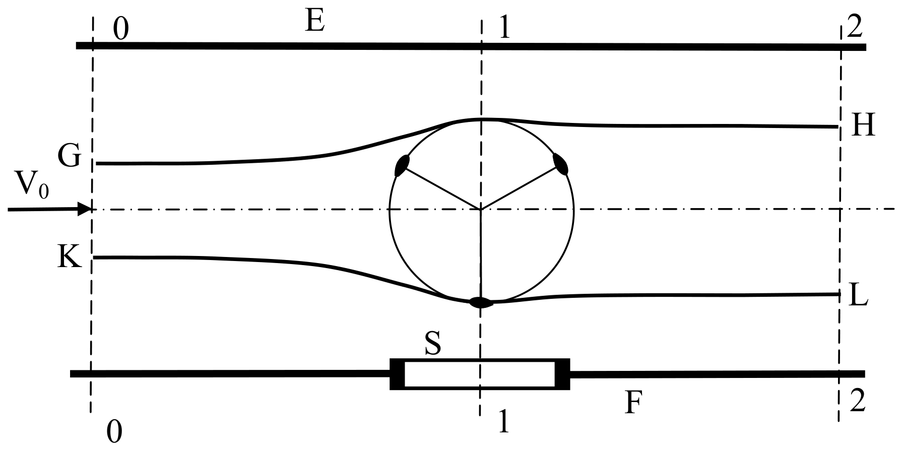
The study of the structure of the flow around the rotor model of a wind turbine was carried out in a hydrodynamic tube GT-400 of TsAGI named after N. E. Zhukovsky [39]. The main characteristics of the model are diameter D = 0.195 m, blade section profile NACA 0018, quantity of blades N = 3, blade chord b = 0.026 m, blade inclination angle γ = 0, and blade length (rotor height) H = 0.225 m.

Figure 2 shows a schematic diagram of the experimental setup in the GT-400 hydrodynamic tube. The setup includes the rotor model with three blades, water inlet and outlet sections, and a flow visualization system.

Due to the use of an electric motor and a gearbox, the rotation speed of the model could vary from 15 to 25 rpm. The water flow rate with the help of the valve varied from 2 to 7.5 cm/s. The tip speed ratio varied within 2–5, and the Reynolds number in the range 0.5 ∙ 10³–1.7 ∙ 10³.

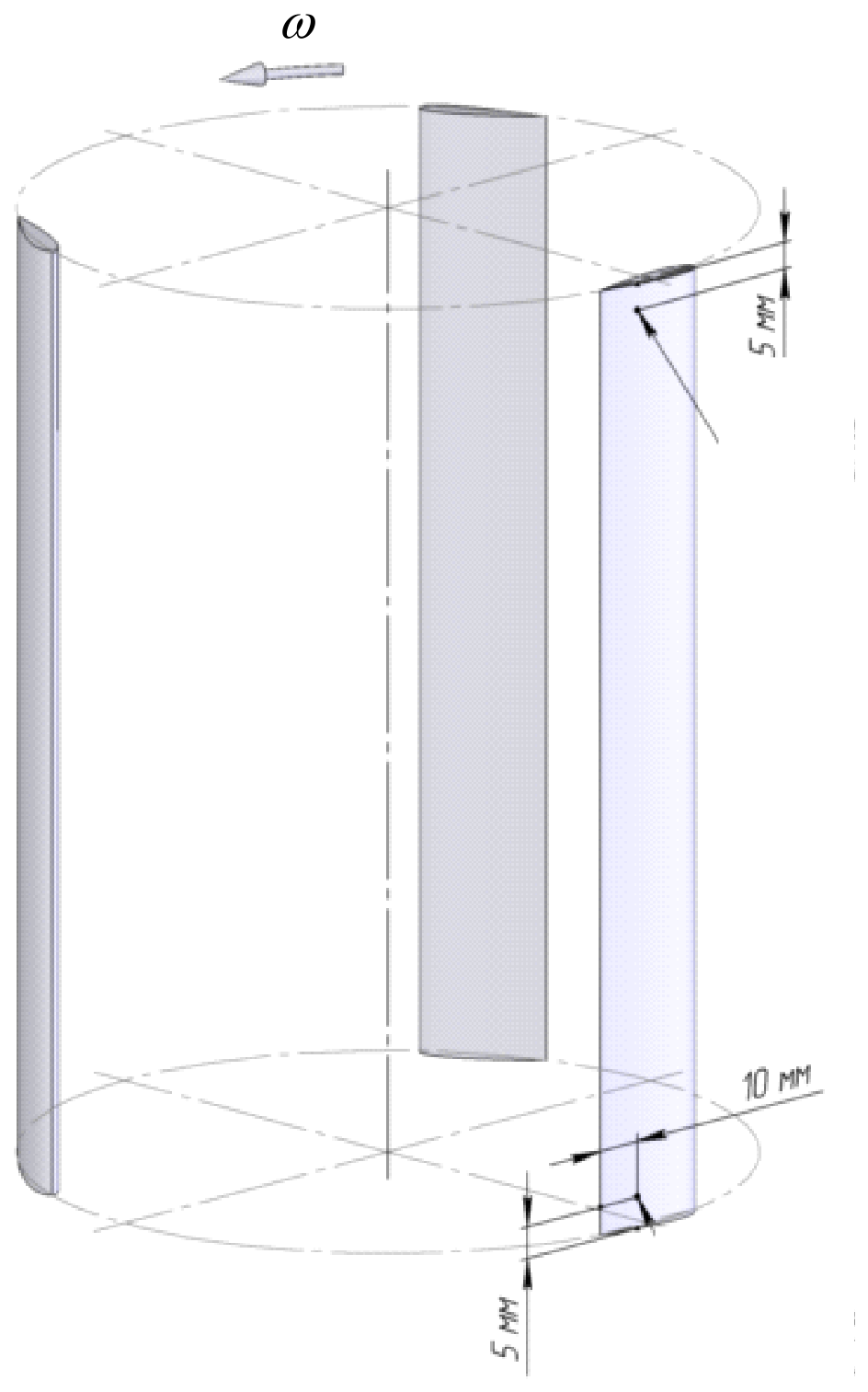
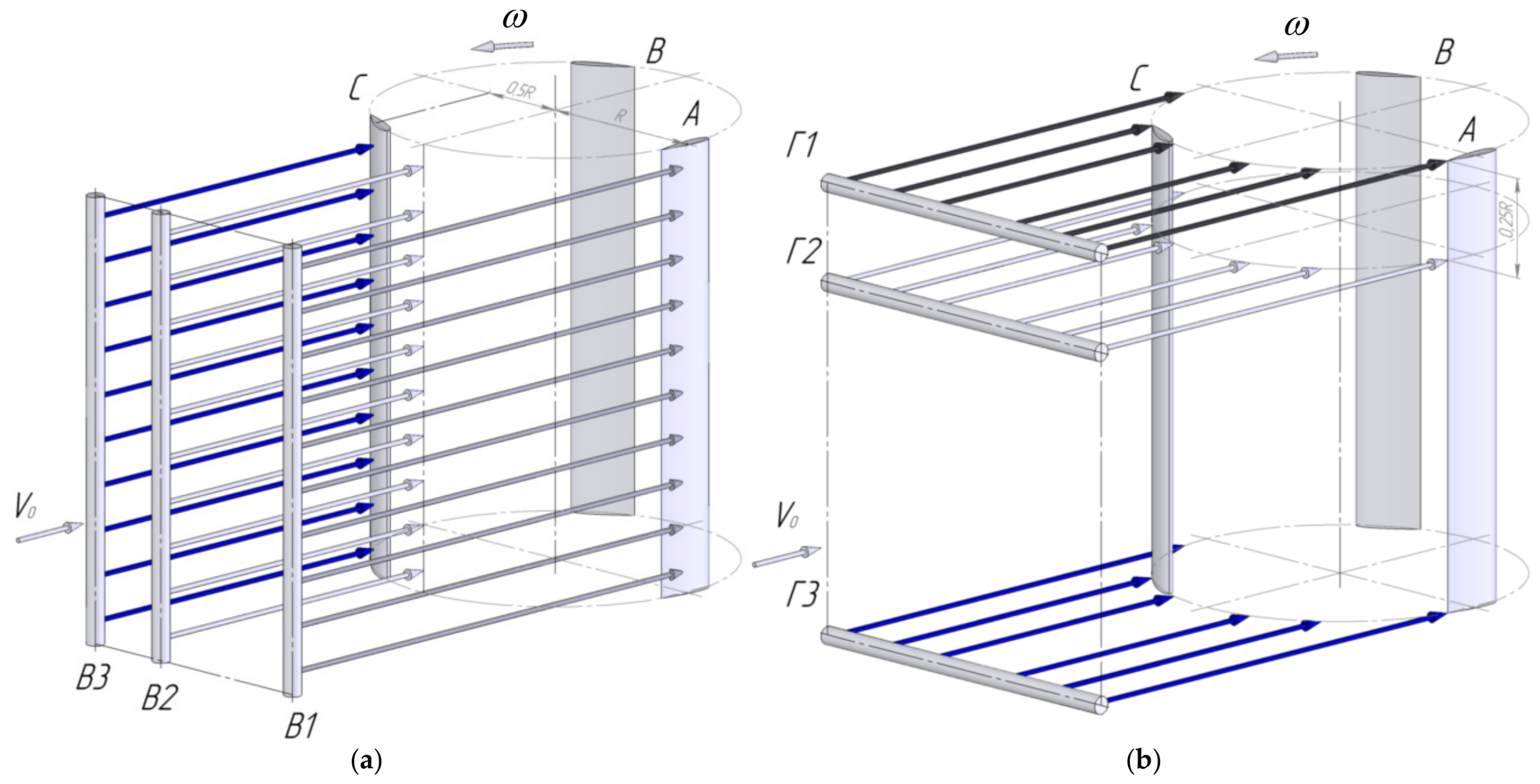
Hydrodynamic spectra were obtained by photographing, and jets of colored liquid were emitted from special combs located both parallel and perpendicular to the axis of rotation of the wind turbine rotor model. Colored jets were also obtained from the end parts of the blades of the wind turbine rotor model. The scheme of holes on the blade is shown in Figure 3. Schemes of vertical combs parallel to the axis of rotation of the model and horizontal combs perpendicular to the axis of rotation of the model are shown in Figure 4.

Visualization of the flow structure was carried out using the colored jet method, which is based on the injection of a colored liquid with a density close to the flow density into the flow. The colored jets clearly show the streamlines and their change under different flow regimes. Jets of colored liquid were released from combs located in front of the model parallel and perpendicular to its axis of rotation, as well as from holes located on the outer surface of the model blades near their ends.

The colored jet method belongs to the group of tracer-based flow visualization techniques, which are well established in experimental fluid mechanics and have long been used to obtain qualitative information about separation, vortex formation, wake development, and other flow structures [40,41].

In studies of vertical-axis wind turbines and Darrieus rotors, tracer-based visualization and particle-image velocimetry have also been used to investigate dynamic stall, leading-edge vortex formation, blade–vortex interaction, and wake evolution [42,43]. For example, dye injection and PIV measurements have previously been applied to study the flow field around a Darrieus rotor under dynamic-stall conditions [42].

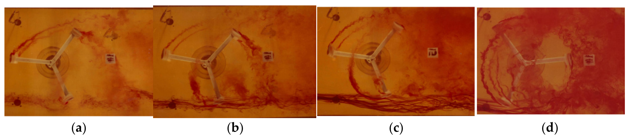
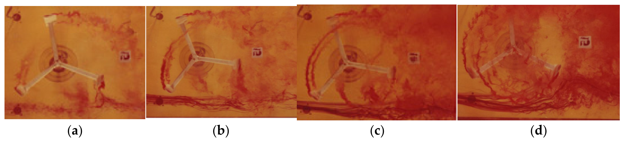
The images were obtained by photographing the patterns of currents from the side (in the vertical plane) and from above the model (in the horizontal plane). To obtain a complete picture of the phenomena, photography of the flow field was carried out in two modes: (I) in chronological sequence with a constant tip speed ratio for various azimuthal positions of the rotor and (II) for one azimuthal position of the rotor at various tip speed ratio.

The location on the blades of two inlet holes in the flow of tinted fluid near the upper and lower ends (Figure 3) allows us to obtain a complete picture of the flow inside the rotor and the trace behind the rotor by visualizing a pair of dynamic flow stall vortices and a pair of vortex traces of each blade in the upper and lower parts of the H-rotor.

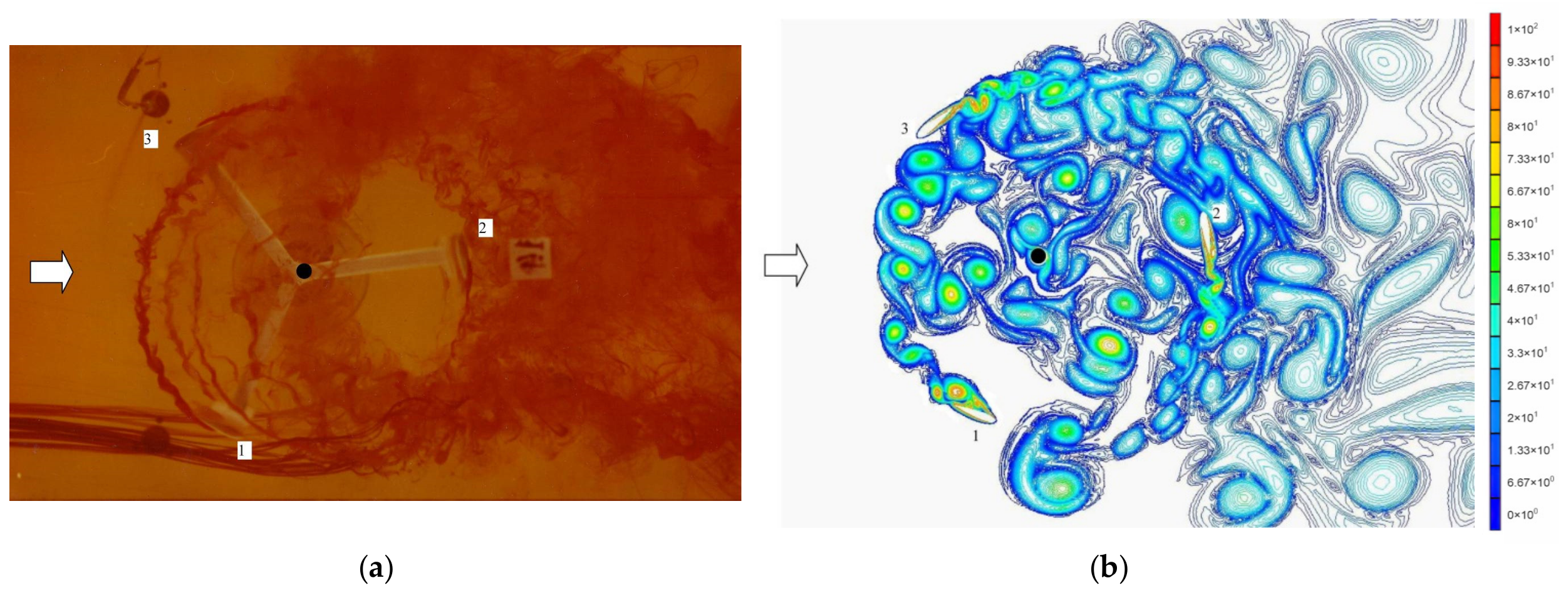
The visualization of the actual flow around the H-rotor was carried out for two verification tasks: first, to confirm the correspondence between the calculated and physical flow and vortex structures on the rotor at a single azimuthal position for different rotor angular velocities (Figure 5a–d); and second, at several consecutive azimuthal positions for a single rotor angular velocity (Figure 5a–d and Figure 6a–d). The calculations and experiments were performed for H-rotor tip speed ratios λ = 2, 3, 4, and 5. In Figure 5 and Figure 6, the flow structure is visualized using colored dye streams released from holes on the upper and lower ends of the blades, as well as from a vertical comb located at the boundary of the flow jet passing through the rotor.

4.2. Description of the Computational Experiment

In the present work, a numerical simulation of the flow around a three-blade Darrieus rotor is performed for the following parameters:

• Angular velocity of rotation—ω = 2 rad/s;
• Water flow velocity—U = 0.065 m/s;
• Blade chord—b = 0.026 m;
• Kinematic viscosity of water at a temperature of 15 °C—ν = 1.15 × 10⁻⁶ m²/s;
• Tip speed ratio—λ = 3;
• Reynolds number—Re = Ub/ν = 1470.

To assess the sensitivity of the numerical solution to spatial and temporal discretization, additional grid- and time-step-sensitivity studies were performed. Such verification procedures are commonly recommended in CFD studies to estimate the influence of discretization errors on the calculated quantities of interest [44,45,46,47].

Three systematically refined computational grids were considered: coarse, medium, and fine. The same numerical scheme, boundary conditions, turbulence model, and convergence criteria were used for all grid levels. The monitored quantities included the averaged torque coefficient (C_Q) and the main qualitative features of the vortex structure during one periodic rotor revolution.

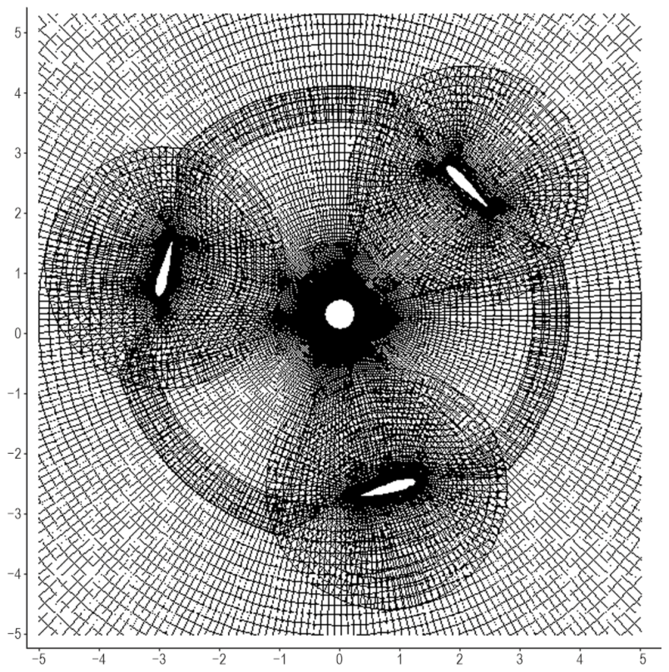
Calculations were carried out on the multi-block (5 blocks) O-type grid with the number of nodes in the radial and circle directions $200\times 200$ (Coarse grid), $300\times 200$, (Medium grid), and $300\times 300$ (Fine grid) respectively with local refinement near the blade surface to capture boundary layer behavior and vortex shedding accurately (Figure 7). The total number of nodes of the multi-block grids were $2.0\times {10}^5$, $3.0\times {10}^5$, $4.5\times {10}^5$. The dimensionless step in time, calculated in the length of the chord and speed of the unperturbed stream, were $\mathrm{\Delta }t=0.01$, $\mathrm{\Delta }t=0.005$, and $\mathrm{\Delta }t=0.0025$.

The results of the grid sensitivity study are summarized in

Table 1. Grid sensitivity study for the Darrieus H-rotor simulation at λ = 3.

Grid Type	Number of Grid Cells	Averaged Torque Coefficient
Coarse	200,000	0.028
Medium	300,000	0.033
Fine	450,000	0.034

. The variation in the monitored averaged torque coefficients between the medium and fine grids was found to be small, indicating that the medium/fine grid resolution provides a sufficiently grid-independent solution for the purposes of the present study. In addition, the main vortex formation, shedding, and convection patterns remained unchanged with further mesh refinement.

A time-step-sensitivity analysis was also performed using three time-step values while keeping the same grid resolution (medium grid). The monitored quantities were averaged torque coefficients and the phase position of the main dynamic-stall vortex. The results are presented in

Table 2. Time-step sensitivity study for the Darrieus H-rotor simulation at λ = 3.

Dimensionless Time Step	Averaged Torque Coefficient
∆t = 0.01	0.041
∆t = 0.005	0.033
∆t = 0.0025	0.032

. The differences between the medium and smallest time steps were minor, confirming that the selected time-step size is adequate for resolving the unsteady vortex dynamics considered in this work.

The uncertainty associated with spatial and temporal discretization was therefore estimated from the relative differences between the refined solutions. The obtained values indicate that the numerical uncertainty is sufficiently small compared with the observed differences in the flow structure caused by dynamic stall. Consequently, the computed vortex patterns and integral aerodynamic quantities can be considered insensitive to further grid and time-step refinement within the accuracy required for the present validation study.

The grid was built by the method of many surfaces. The external boundary of the estimated area was at a distance of 40 chords from the center of the airfoil. The thickening of the nodes was carried out in the direction of normal to the surface, as well as to the front and extreme parts of the profile. In the border layer there were about 100 points, which provided adequate resolution of parietal effects.

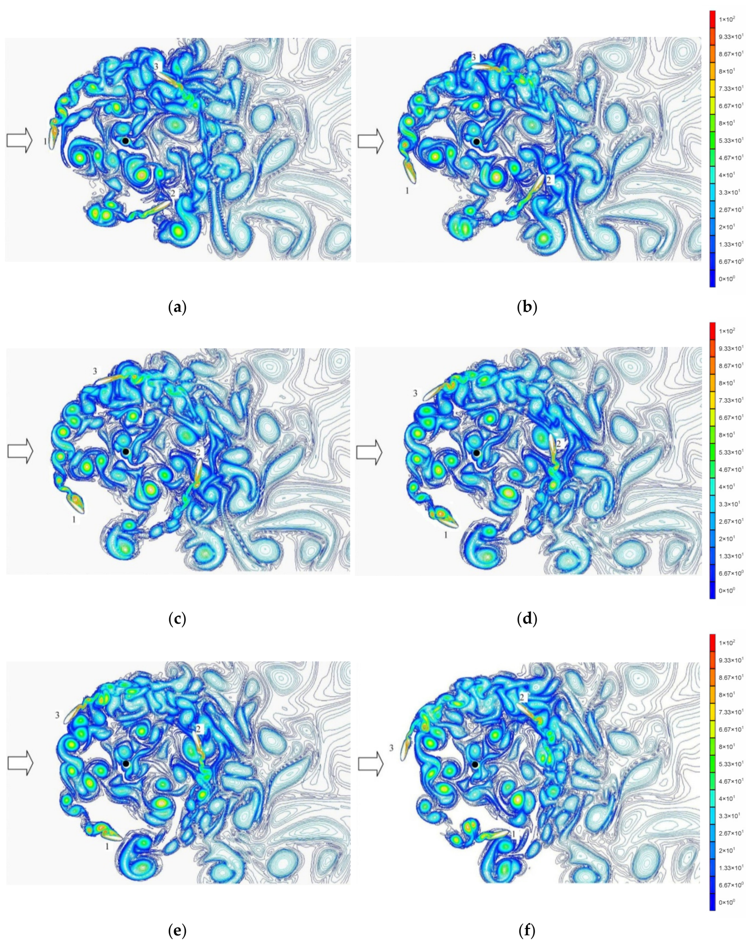
After the three-blade Darrieus rotor enters the periodic flow around (the period is 120°), the stages of nucleation, development, separation and dissipation of vortices in different sections of the blade trajectory are singled out. The value of the angle θ = 0° corresponds to the position of the rotor when the first blade is located perpendicular to the oncoming flow in the windward part of the trajectory.

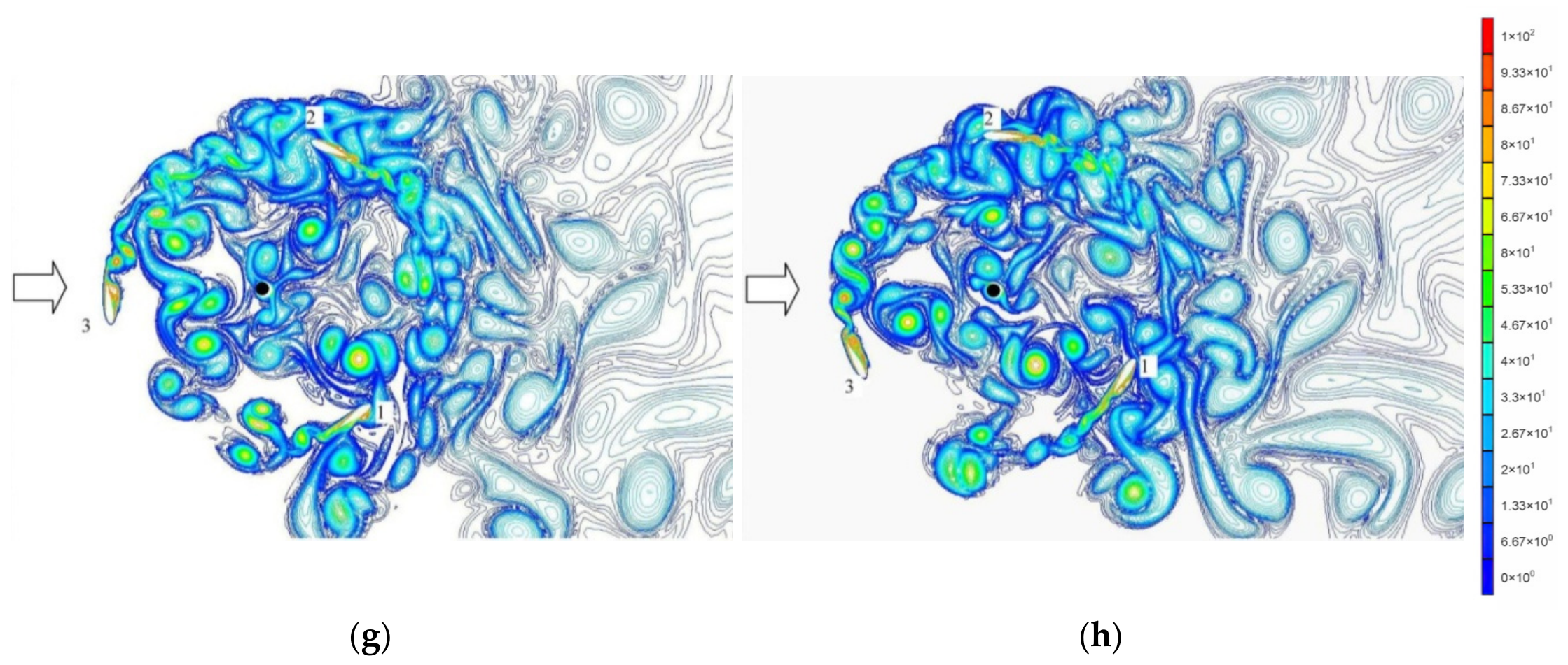
Based on the analysis of the vorticity contours in Figure 8a, at the angle of rotation of the first blade θ = 0° (the local angle of attack of the blade is α = −19°), a dynamic separation of the flow occurs on the inner surface. The boundary layer is torn off near the trailing edge, and the position of the separation point is shifted towards the leading edge of the blade. This leads to the separation of the vortex from the nose of the blade and subsequent movement along the chord towards the trailing edge. Vortices are formed on the tip of the blade 1, which then move along the surface in Figure 8b–d.

It is important to note that the vorticity contours and flow visualizations presented in Figure 8, Figure 9, Figure 10, Figure 11 and Figure 12 provide qualitative insights into the flow structure. For quantitative velocity data, appropriate legends and scales would be incorporated.

At an angle of rotation of the rotor of 80°, the dynamic shedding of vortices is suppressed, and flow reattachment begins (Figure 8e). The process starts near the leading edge and moves towards the trailing edge. The shedding of vortices from the inner surface of the first blade is observed until the angular position of the rotor approaches 90°.

At the beginning of the leeward section of the trajectory θ = 90° and up to the angular position of the rotor θ = 120°, the flow around blade 1 has an attached character (Figure 8f). Flow separation begins at the angular position of the rotor θ = 120°, which corresponds to the local angle of attack of the blade α = 17° on Figure 8g. As in the case of dynamic stall from the inner surface, the vortices break off from the leading edge of the blade and begin to move along the surface on Figure 8g–h. At the rotor rotation angle θ = 120° on Figure 8h, the position of the first blade corresponds to the position of blade 3 at θ = 0. The flow reattaches to the surface of blade 2 when the rotor rotation angle is θ = 310° on Figure 8g. A periodic flow begins to form in the wake, resembling a von Karman vortex street behind a cylinder in structure.

With the tip speed ratio λ = 3, dynamic separation of the flow from the blade of the Darrieus rotor is observed on most of the trajectory. It is characterized by separation of the flow from the leading edge of the blade and the formation of large vortex structures that are carried along the chord of the blade.

The change in absolute velocity along the circumference of rotation of the blade leads to a larger area of dynamic stall in that part of the trajectory where the blade and flow velocities are in the same direction. In this zone, the oncoming flow carries the vortices in the direction of the blade movement. On the second half of the trajectory, the flow carries the vortices in the direction opposite to the movement of the blade. In this case, the duration of the dynamic stall is less than in the previous one.

The main reason for the dominance of dynamic vortex shedding over most of the blade trajectory is the low Reynolds number Re = 1470, which corresponds to the initial stage of the transition from laminar to turbulent flow.

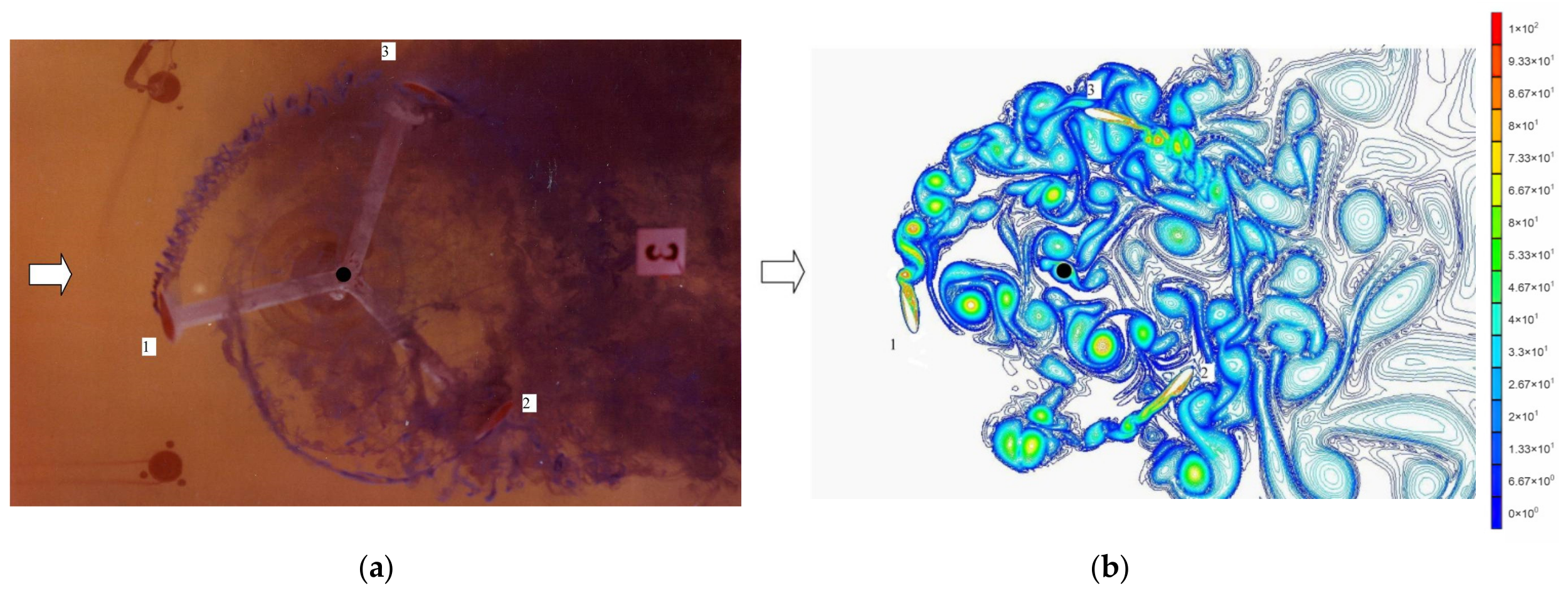
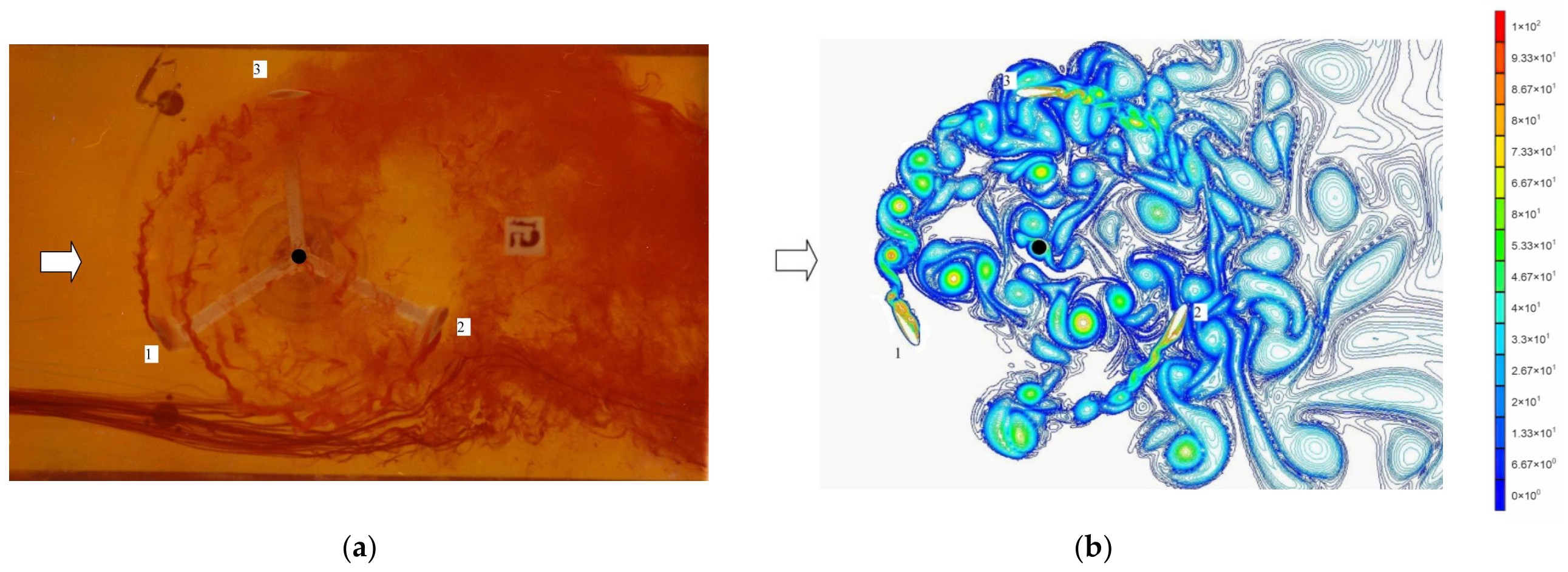
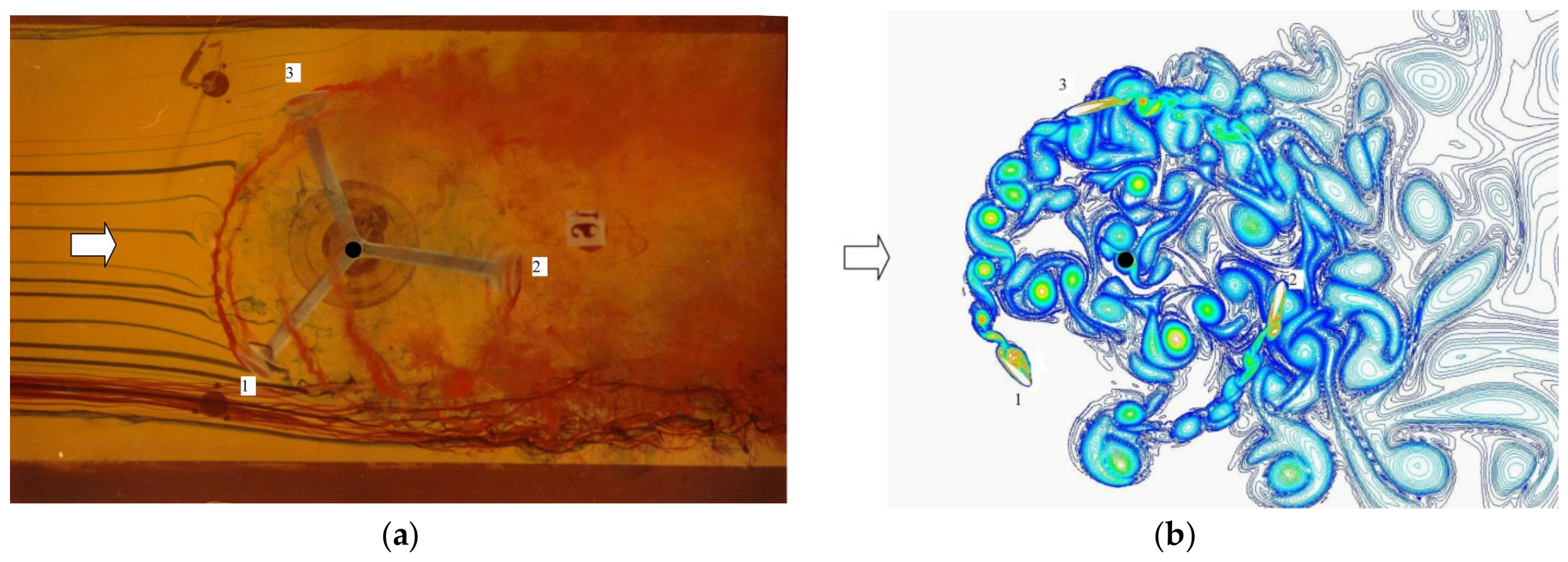
As a result of the physical experiment carried out in [39], instantaneous patterns of the flow around a three-blade Darrieus rotor were obtained. Figure 9, Figure 10, Figure 11 and Figure 12 show pictures obtained while filming from the end of the working model of the wind turbine rotor, which demonstrates the processes of formation and diffusion of vortices that have descended from the ends of the blades, at various angular positions of the blade and at the tip speed ratio value λ = 3. Let us analyze the patterns of flow visualization during the operation of the Darrieus rotor under conditions of dynamic flow separation on the basis of natural (a) and computational (b) experiments.

The instantaneous flow pattern is characterized by the presence of a system of large eddies that rotate in opposite directions. With the tip speed ratio λ = 3, there is an asymmetry between different sections of the blade trajectory.

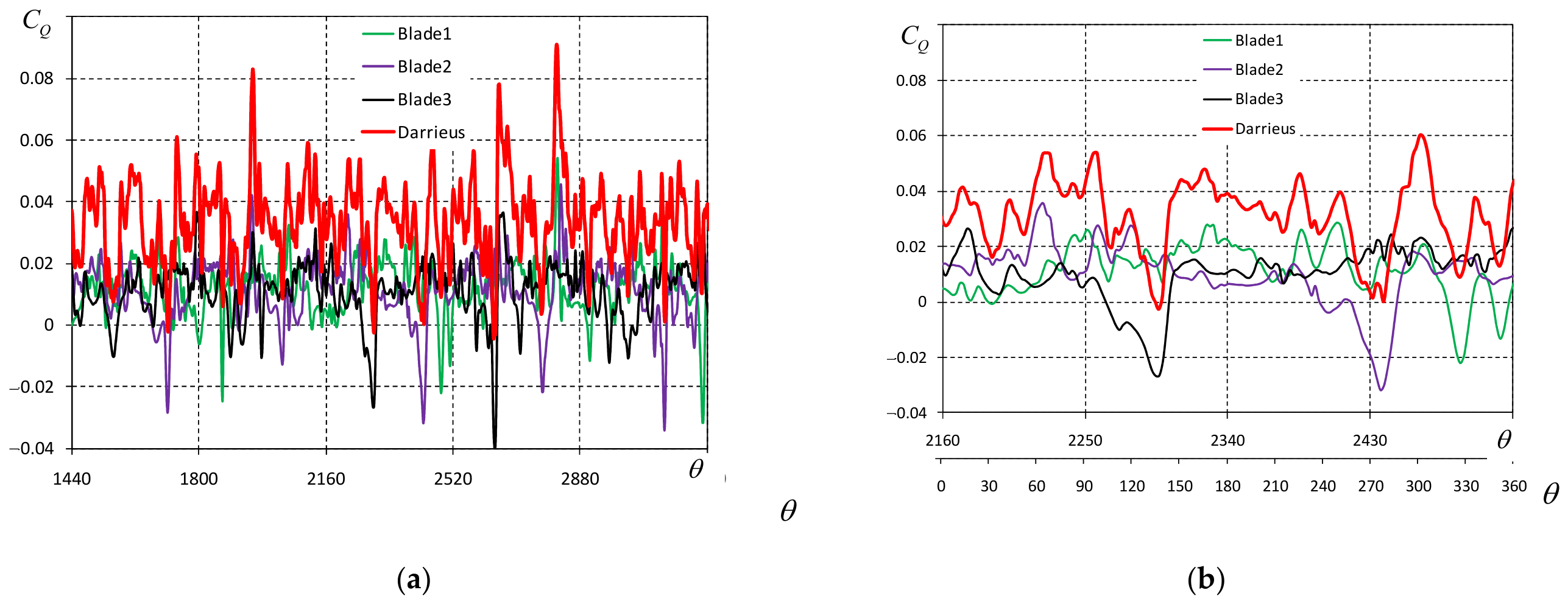
The dependence of non-averaged coefficients of torque C_Q on the angular position of the blades and Darrieus rotor at the tip speed ratio λ = 3 are shown in Figure 13. The values of the torque and power coefficients of a three blade of the Darrieus rotor averaged over one revolution have the following values ${\overline{C}}_Q=0.033$ and ${\overline{C}}_P=0.1$, respectively. This value is consistent with published data for low Reynolds number operation and supports the suitability of the rotor design for low-speed flow conditions.

5. Discussion

The instantaneous flow pattern is characterized by the presence of a system of large eddies that rotate in opposite directions. With the tip speed ratio λ = 3, there is an asymmetry between different sections of the blade trajectory. The vortices that have descended from the blades, moving towards the flow, in most cases have a greater intensity than the vortices that have descended from the blades, moving along the flow. This is explained by the fact that the relative flow velocity in this section of the blade trajectory is higher than in the opposite one. Downstream, traces of vortex concentrations from the blades moving downstream are visible after some of their diffusion.

Visualization of the flow structure for various azimuthal positions of the rotor model is shown in Figure 9, Figure 10, Figure 11 and Figure 12. So, in Figure 9, in the front part of the rotor model of the wind turbine, there are clusters of vortices that have descended from the first blade. Further downstream, clusters of vortices that have descended from the previous blades are visible.

A positive effect was found when the colorants were released not from the ends, as was the case during the previous work, but from holes located at a distance of 0.02 half-span of the rotor blades. There is an asymmetry in the size and speed of the vortices between the upper and lower (relative to the X axis) parts of the rotor. The lower region is characterized by the presence of large vortex structures, which are the result of dynamic separation of the flow from the inner surface of the blade. The upper region is the vortices of medium intensity in the wake behind the blade. This is explained by the fact that in the first case, the vortices are pushed by the blades moving along the flow, and in the second case, on the contrary, they are slowed down due to the action of viscous effects.

The resulting system of vortices affects the flow structure near the blades of the Darrieus rotor. Vortices that have escaped from the leading blade create turbulence of the flow for the blade following it.

During one revolution, the flow velocity relative to the blade profile changes cyclically in magnitude and direction. In engineering methods, the absolute speed of the oncoming flow is assumed to be equal to the vector sum of the velocities of the blade and the wind. In fact, this speed also depends on the speed of the vortices that have descended from the blades and the rotor support tower. The non-stationary effects caused by the interaction of the vortex system with the blade play a significant role in determining the aerodynamic forces acting on the rotor.

In general, the flow pattern near the Darrieus rotor is characterized by significant non-stationary phenomena. These include: dynamic stall, the formation of a complex system of vortices, an increase in the level of turbulence in the shaded area, the interaction of vortices of various sizes, speeds and intensities with the solid surfaces of the wind turbine rotors. The resulting flow pattern is in good agreement with the available experimental data.

In the presence of complex interrelated non-stationary effects, to calculate the aerodynamic forces acting on the rotors, methods should be used that can adequately convey the real structure of the flow. The results obtained will allow a deeper understanding of the physical processes occurring during the operation of the Darrieus rotor of a vertical-axial wind turbine, and can also be used to improve existing schemes and select efficient wind turbine designs.

While the vorticity distribution provides valuable insights into dynamic stall, future work will involve presenting the hysteresis cycles of hydrodynamic parameters such as lift and drag coefficients to further quantify and discuss the dynamic stall phenomena more comprehensively.

In addition to the qualitative comparison of vortex structures, a quantitative assessment of the numerical results was performed in order to evaluate the engineering relevance of the proposed modeling approach.

For the investigated operating condition (λ = 3), the computed averaged power coefficient was Cp = 0.1, while the mean torque coefficient was Cq = 0.3. The obtained value is consistent with the low-Reynolds-number operating regime of the investigated model and falls within the range reported in previous experimental and numerical studies of Darrieus-type vertical-axis wind turbines operating under comparable low-Reynolds-number or dynamic-stall conditions [24,25,27,29,30,48,49].

Table 3. Comparison of the present results with published studies of Darrieus-type VAWTs.

Study	Method	Rotor/Airfoil	Reynolds Number	TSR	Reported Quantity	Value/Range	Comment
Present study	URANS-SALSA + experiment	3-bladed H-rotor, NACA 0018	1470	3 2–5 (experiment)	Cp, Cq	Cp = 0.01	Hydrodynamic-channel validation
Strickland et al. [25]	Analytical + experimental	Darrieus rotor	40,000	1–5	Cp, forces/vortex behavior	Cp = 0.01–0.3	Classical Darrieus benchmark
Rezaeiha et al. [27]	URANS/SAS/hybrid RANS-LES	VAWT	50,000	2–3	Dynamic stall, loads, vortex structures	Cp = 0.1–0.3	CFD comparison for dynamic stall
Le Fouest and Mulleners [29]	Experiment	VAWT blade	50,000	1.2–6	Load and velocity-field data	Cp = 0.1–0.3	Dynamic-stall regimes
Rogowski et al. [48]	CFD/airfoil data	NACA 0018	160,000	4.5	Lift/drag coefficients		Low-Re NACA 0018 reference
Ridho and Prabowo [49]	CFD + experiment	H-Darrieus VAWT	50,000– 15,000	0–0.3	Cp, Cq	Cp = 0–0.1	H-Darrieus validation case

compares the present numerical results with available published data. It should be noted that the comparison is not expected to be exact because the referenced studies differ in rotor geometry, Reynolds number, solidity, blade airfoil, turbulence model, and experimental or numerical setup. Nevertheless, the comparison provides an additional quantitative benchmark and supports the reliability of the predicted order of magnitude of the aerodynamic performance.

The comparison confirms that the calculated integral performance characteristics are physically plausible for the considered low-Reynolds-number regime. In addition, the predicted stages of dynamic stall, including vortex formation near the leading edge, vortex growth, shedding, and downstream convection, are consistent with the experimentally observed dynamic-stall mechanisms reported in previous studies [29,30].

Therefore, the validation of the present model is based on three complementary elements: (i) comparison of the calculated and experimentally visualized vortex structures, (ii) quantitative evaluation of integral aerodynamic coefficients, and (iii) comparison with published experimental and numerical studies. Although more detailed validation using PIV velocity fields or direct force measurements would further strengthen the analysis, the present results demonstrate that the URANS-SALSA approach is capable of reproducing the dominant flow physics and the basic performance characteristics of the investigated Darrieus H-rotor.

6. Conclusions

The problem of selecting a modeling method for the flow around Darrieus H-rotors from the standpoint of practical engineering design has been formulated. The proposed approach represents a compromise between adequately capturing the main aerodynamic effects and being accessible for implementation in engineering practice. Verification showed that the model of aerodynamic processes of Darrieus H-rotors, based on the Reynolds-averaged Navier–Stokes equations for an incompressible fluid and complemented by the one-equation differential Spalart–Allmaras turbulence model adapted to the strain tensor, adequately describes the main aerodynamic effects during the flow around a Darrieus H-rotor.

The analysis of the flow field around a three-bladed Darrieus H-rotor at λ = 3, carried out during the verification process and based on a comparison of experimental flow visualization and numerical simulation of vortex dynamics, showed that dynamic stall occurs along most of the rotor trajectory in the experimentally obtained flow patterns. Dynamic stall is characterized by flow separation from the leading edge of the H-rotor blade and the formation of large vortex structures that are advected along the blade chord. It was confirmed that the developed software package allows the reproduction of real aerodynamic processes during the rotation of vertical-axis wind turbine (VAWT) rotors.

Of particular value to researchers are the original and rather unique experimentally obtained flow visualization results from the hydrodynamic channel tests of the three-bladed Darrieus H-rotor at tip speed ratios λ = 2, 3, 4, and 5.

It is assumed that the research should be continued toward studying the physical flow patterns around the considered rotors at different blade pitch angles and during acceleration, operation in the generating mode at various wind speeds, and braking mode, with the aim of improving their aerodynamic and energy characteristics by varying the rotor rotational speed to maintain maximum output power.

The direction of further research will involve the extension of the developed CFD package to solve three-dimensional problems, taking into account the influence of spatial effects, modeling of large-scale turbulence, and optimization of the Darrieus H-rotor shape while maintaining the balance between sufficient simplicity and accuracy achieved during the development of this model.