Assessment of Injection Modeling Techniques for a Water Spray Using an Euler/Lagrange Approach

Abstract

In the context of aircraft engine technologies, sprays are used to inject water into the engine cycle to enhance efficiency and reduce emissions. Accurate specification of droplet injection boundary conditions is therefore essential for reliable numerical predictions. This study presents a numerical validation of a water spray configuration previously characterized using phase Doppler anemometry. An Euler/Lagrange approach is applied to simulate the spray using two distinct injection strategies: an array of injector points (Case 1) and a solid-cone injector (Case 2). Numerical results are compared with experimental data to assess droplet size and velocity distributions. Both approaches capture the main spray characteristics, while Case 1 provides improved agreement due to a more accurate representation of the injection conditions. In addition, the influence of droplet–droplet collisions is investigated using different collision-regime maps. While the collision models lead to significantly different collision outcomes, only minor differences are observed in spray characteristics, with noticeable deviations occurring in the downstream region. Overall, the results demonstrate the importance of accurate injection modeling for reliable spray predictions, while simpler injection approaches remain viable with reduced accuracy. The influence of collision modeling is limited under the present conditions and for the investigated spray metrics, providing insight into its role and limitations in polydisperse sprays.

1. Introduction

A spray is a dispersed two-phase flow consisting of liquid droplets distributed within a continuous gas phase, typically produced by the atomization of a liquid jet or sheet. Sprays are used in numerous engineering applications, including cooling, combustion, coating, and air humidification. While these processes serve different purposes, a common objective is to control droplet size distribution to optimize heat and mass transfer. In addition to their technical relevance, sprays are often investigated in fundamental studies to improve the understanding of droplet dynamics and multi-phase flow behavior.

Depending on the region of interest within a spray and the dominant physical phenomena, different experimental approaches are employed to investigate the spray behavior. Optical measurement techniques are widely used in the literature, as they enable non-intrusive characterization without disturbing the spray dynamics. In the dense near-field region of a spray nozzle, where macroscopic spray characteristics (e.g., cone angle, penetration length, spray width and overall spray shape) are of interest, shadowgraphy and schlieren imaging are typically applied. In contrast, in the dilute far-field region, where the liquid phase consists of dispersed droplets, phase Doppler anemometry (PDA) is a widely used technique to quantitatively characterize droplet dynamics (e.g., droplet size and velocity) within the spray. Fansler and Parrish [1] provide a comprehensive review of available spray diagnostics and highlight the most suitable techniques for each of the principal spray regions.

In many applications, the surrounding conditions are complex, making the detailed characterization of spray behavior challenging. Modern experimental diagnostics provide valuable insight, but numerical simulations are often used alongside experiments to obtain complementary information about the underlying flow and droplet dynamics. Mainly two approaches exist to model sprays: Euler/Euler methods, which treat sprays as a continuous phase and are suited for dense spray regions and breakup processes, and Euler/Lagrange methods, which track individual droplets and better capture their trajectories and interactions [2]. In both cases, however, the gas flow is treated as a continuous phase using the Eulerian framework. To accurately model the continuous airflow, appropriate turbulence modeling is essential. Common approaches for the continuous phase in spray simulations include direct numerical simulation (DNS), large-eddy simulation (LES), and eddy-viscosity models based on the Reynolds-averaged Navier–Stokes (RANS) equations. DNS is computationally very expensive for practical spray applications and is therefore not feasible for complex or large domains. LES provides higher fidelity by resolving the large turbulent structures, but still demands significant computational resources. In contrast, RANS models remain the most practical choice for engineering-scale spray simulations, offering a reasonable balance between accuracy and computational cost. Within the Euler/Euler framework, the phase interface can be either fully resolved using the Volume of Fluid (VOF) method or left unresolved using a two-fluid model. The VOF method enables the resolution of the free surface of a liquid phase to study spray phenomena (e.g., breakup processes) and instability in detail. Liu et al. [3] used LES-VOF simulations to analyze the primary breakup of high-speed liquid jets. Similarly, Hu et al. [4] employed this method to investigate the influence of internal nozzle flow patterns and cavitation structures on the primary breakup and atomization quality of fuel sprays. Furthermore, Karpiński et al. [5] conducted a RANS-VOF approach to analyze pressure, velocity and turbulence characteristics in a hollow-cone nozzle. Although the VOF method is a suitable approach to analyze resolved spray phenomena in detail, it has disadvantages in terms of computational cost and numerical stability, as very fine numerical grids are required to resolve small-scale features. Two-fluid (Euler/Euler) modeling approaches provide a computationally efficient alternative to fully resolved interface tracking for simulating the dense near-nozzle spray region, including in-nozzle flow and primary liquid-jet or sheet breakup, before transitioning to a Lagrangian description of the dispersed spray further downstream [6]. These methods treat all phases as interpenetrating continua, solving separate transport equations for each phase while sharing a common pressure field. Inter-phase interactions arising from Eulerian averaging require closure models for drag, lift, and heat transfer [7]. Devassy et al. [8] developed an Eulerian/Eulerian two-fluid model for diesel jet atomization, capturing primary breakup and demonstrated good agreement with DNS results under engine-relevant conditions.

While two-fluid models provide a computationally efficient representation of the dense, near-nozzle region, they inherently lose information about individual droplet trajectories once the liquid jet has broken up and the phases become fully dispersed. In contrast, the VOF method preserves interface details but becomes numerically too expensive for simulating the larger downstream regions where the dispersed droplet phase dominates. For this reason, Euler/Lagrange methods are widely employed in spray simulations, as they allow the tracking of individual droplets beyond the primary atomization zone. A key requirement for accurate Euler/Lagrange simulations is the definition of a suitable spray injection boundary condition, since all subsequent droplet trajectories and interactions depend on the initial size, velocity, angle, and spatial distribution assigned at the injection plane. A variety of strategies exist in the literature to construct such boundary conditions. For instance, Qin and Loth [9] injected droplets at a plane 9 mm downstream of a pressure-swirl nozzle, prescribing droplet-size distributions and velocity profiles obtained from PDA measurements at that location. Similarly, Lain and Sommerfeld [2] examined the influence of different collision models on spray dynamics prescribing measured droplet-size distributions and velocity profiles at a plane 25 mm downstream of a hollow-cone nozzle. Enderle et al. [10] reconstructed spray boundary conditions by projecting PDA data from a measurement plane 15 mm downstream of the hollow-cone pressure swirl atomizer back to the computational inlet, prescribing Rosin–Rammler droplet sizes and assigning droplet velocities according to measured velocity distribution functions. In fire-safety applications, Beji et al. [11] injected droplets from a spherical surface at a prescribed location using measured volume-flux distributions and a combined Rosin–Rammler/lognormal size distribution. The initial velocities were computed from the nozzle operating pressure using an empirical correlation, and droplet directions were sampled from an angular probability distribution representing the spray cone. In high-pressure diesel applications, Shi and Kleinstreuer [12] imposed injection directly at the nozzle exit, using a blob-model droplet diameter in combination with empirical relations for the initial droplet velocity and spray cone angle. For hollow-cone and pressure-swirl atomizers, studies such as by Treleaven et al. [13] and Sanjosé et al. [14] defined injection on ring-shaped surfaces that approximate the breakup of the swirling liquid sheet, assigning droplet sizes from measured or fitted Rosin–Rammler distributions and prescribing injection angles consistent with the observed spray geometry. Likewise, for multi-hole gasoline injectors, Gerbino et al. [15] demonstrated that the selected initial droplet-size probability distribution can significantly influence plume penetration and spray shape, even when the nozzle geometry is fully known. However, the reviewed studies show that defining suitable injection boundary conditions for Euler/Lagrange simulations is highly case dependent. Existing approaches typically rely on downstream measurement data, empirical correlations for velocity and spray angle, or idealized geometric representations of the breakup region, and their applicability is limited when experimental data are sparse or available only at selected locations. Motivated by these limitations, the present work investigates how such strategies can be transferred and adapted to a hollow-cone water spray.

Motivated by these considerations, the present study examines a practical application in which reliable spray injection conditions are equally essential. Sprays also play an important role in the context of aircraft engine technologies, where fuel is injected into the combustor or water is introduced into the engine cycle to enhance efficiency and reduce emissions [16]. For this concept, the injected water needs to be separated from the exhaust gas. At the Institute of Aerospace Thermodynamics (ITLR) of the University of Stuttgart, the fundamental physics of water separation from an airflow are investigated in detail by performing experiments and numerical multi-phase flow simulations in a channel flow operated with saturated air and liquid water. To inject water into this channel, hollow-cone injectors are used. A valid boundary condition for the injection of droplets is essential to accurately predict spray behavior in numerical simulations. Therefore, the main objective of this work is to implement and validate a numerical model for the droplet injection using a similar water spray studied by Rüger et al. [17], where droplet size and velocity distributions were measured using PDA. The numerical simulation of the spray is conducted using the STAR-CCM+ software (version 2506) with an Euler/Lagrangian approach. Because detailed internal nozzle information is not available, simplified injection models are often used to reproduce experimentally observed spray characteristics. In engineering applications, complete experimental boundary conditions and detailed nozzle information are often unavailable. Therefore, the present work focuses on the practical implementation and validation of simplified injection models for spray simulations within a commercial CFD framework. In this study, two different injection modeling strategies are evaluated for reproducing the experimentally observed hollow-cone spray. In the first approach (Case 1), an array of injector points is used to introduce discrete droplet parcels with predefined sizes and velocities at a plane located 25 mm downstream of the nozzle, following the downstream-injection strategy proposed by [2]. In the second approach (Case 2), a simplified semi-empirical solid-cone injector model is employed at the nozzle exit. This model does not represent the physical injector geometry but serves as a surrogate injection model to reproduce the measured spray characteristics. The resulting droplet size and velocity distributions are compared against experimental data to assess the predictive accuracy of each method.

Table 1. Positioning of the present study relative to the work of Lain and Sommerfeld [2].

Aspect	Lain and Sommerfeld [2]	Present Study
Objective	Influence of collision maps on spray evolution	Validation of two injection modeling strategies and assessment of collision-map influence
Injection	PDA-based downstream injection	PDA-based downstream ring injection and simplified solid-cone injector
Implementation	Euler/Lagrange framework	STAR-CCM+ Euler/Lagrange framework

summarizes the positioning of the present study relative to the work of Lain and Sommerfeld [2], which represents one of the most closely related numerical investigations based on the experimental spray data of Rüger et al. [17].

Furthermore, the influence of droplet collisions on the downstream spray evolution is investigated, with particular focus on the sensitivity of different collision-regime maps to the droplet size ratio $\Delta$ and their influence on both local radial spray characteristics and cross-sectional averaged spray quantities.

2. Numerical Setup and Validation Approach

Figure 1 shows the experimental setup from Rüger et al. [17], which is a $1\mathrm{m}$ long cylinder with a $0.4\mathrm{m}$ diameter. Rüger et al. [17] observed the characteristics of two hollow-cone sprays with different cone angles using PDA measurements. The airflow velocity profiles, liquid mass flow rates, and droplet size and velocity distributions were measured at different radial positions and in four sections downstream of the spray nozzle, as illustrated in Figure 1. The corresponding PDA measurement sections are located at $z=25$, 50, 100, and $200\mathrm{mm}$ downstream of the nozzle.

Table 2. Axial and radial extent of the PDA measurement sections used for validation.

Section	Axial Position z [mm]	Radial Range r [mm]
1	25	0–30
2	50	0–48
3	100	0–75
4	200	0–96

summarizes the radial extent of the measurements within each section used for the validation of the numerical results. The present validation primarily focuses on local droplet size distributions, droplet velocities, and mean droplet diameters. The first measurement section was positioned at $z=25\mathrm{mm}$ downstream of the spray nozzle, ensuring a fully developed spray with primary breakup largely completed, making a modeling of primary breakup unnecessary. The experimental data in this plane provide the foundation for defining the inlet boundary condition in the numerical setup, see Section 2.2.1. As illustrated in Figure 2, the corresponding numerical domain consists of a cylinder with approximately 1,629,500 cells featuring a coarse structured grid in the outer region ($r\ge 100\mathrm{mm}$), a medium unstructured polyhedral mesh in the intermediate region ($30\mathrm{mm}\le r\le 100\mathrm{mm}$) and a fine unstructured polyhedral mesh in the inner region of the spray injection ($0\mathrm{mm}\le r\le 30\mathrm{mm}$), as shown in Figure 2. This meshing strategy ensures sufficient resolution of the high gas-velocity gradients in the core flow and along the spray boundary while keeping the computational cost reasonable. The robustness of the numerical grid was additionally confirmed through a mesh-refinement study based on the Grid Convergence Index (GCI) procedure proposed by Celik et al. [18]. The results showed only small variations in the airflow velocities and droplet mean diameters, as shown in Figure A1. A detailed description of the grid study is provided in the Appendix A. A three-dimensional Euler/Lagrange approach is applied to simulate the dispersed two-phase flow. The carrier airflow is modeled using the Eulerian method, while the Lagrangian approach is used to track droplets.

2.1. Modeling the Single-Phase Flow

In the first step, steady-state single-phase flow simulations without the disperse phase are performed for the airflow and used later as an initial solution for the unsteady multi-phase flow simulations. Within this approach, the airflow is modeled as an incompressible flow for which the governing mass and momentum equations are solved. The turbulent airflow is modeled using the Reynolds averaged Navier–Stokes equations (RANS) in STAR-CCM+. Turbulence is described by the LAG Elliptic Blending k-ε turbulence model [19] in combination with wall functions and no-slip conditions at the cylinder walls. For the lower boundary of the cylinder, a Neumann boundary condition is applied, enforcing zero gradients for all flow quantities. At the upper boundary, a Dirichlet boundary condition is imposed, prescribing the velocity components as well as the turbulent kinetic energy k and its dissipation rate $\epsilon$. Assuming that small droplets follow the gas flow and that their inertial effects can be neglected, these boundary values are estimated from the measured velocities of the smallest droplets obtained from the PDA measurements by Rüger et al. [17]. The turbulent kinetic energy k is obtained from $k=1/2(\overline{u^{\prime 2}}+2\overline{v^{\prime 2}})$, where $\sqrt{\overline{u^{\prime 2}}}$ and $\sqrt{\overline{v^{\prime 2}}}$ are the two measured RMS values of the axial and radial velocity, respectively. Here the RMS value of the circumferential velocity is assumed to be in the same order as that for the radial velocity $\overline{w^{\prime 2}}=\overline{v^{\prime 2}}$. The turbulent dissipation rate is calculated from the turbulent kinetic energy k and a characteristic turbulent length scale $l_e$. While Rüger et al. [17] set the turbulent length scale to $l_e=0.5\mathrm{mm}$, Lain and Sommerfeld [2] chose $l_e=12\mathrm{mm}$ for the same spray. In this work, the turbulent dissipation rate is computed using $\epsilon =k^{1.5}/l_e$, with $l_e$ set to $12\mathrm{mm}$. The value $l_e=0.5\mathrm{mm}$ reported by Rüger et al. [17] corresponds to a nozzle-scale length and, when used in $\epsilon =k^{3/2}/l_e$, leads to a substantially higher dissipation rate. Since the present Euler/Lagrange simulation introduces droplets at $z=25\mathrm{mm}$, $l_e=12\mathrm{mm}$ was adopted as an effective turbulent length scale for the already developed spray region rather than as a nozzle-scale parameter, consistent with the approach of Lain and Sommerfeld [2]. In addition, a sensitivity study with respect to the turbulent length scale was performed. Comparisons of the predicted RMS droplet velocities for different values of $l_e$ showed improved agreement with the experimental PDA data for $l_e=12\mathrm{mm}$. The corresponding results are provided in Figure A2.

2.2. Modeling the Multi-Phase Flow

Following the steady-state single-phase flow simulation without the disperse phase, its solution is utilized as the initial state for the subsequent unsteady multi-phase flow simulation, employing an Euler/Lagrange approach. According to Elghobashi [20], for volume fractions higher than ${\alpha }_p\ge {10}^{-6}$, the influence of the dispersed phase on the continuous gas flow needs to be considered. In the present study however, the mean volume fractions are ${\alpha }_p\approx {10}^{-5}$. Therefore, a two-way coupling approach is applied to account for the interactions between the two phases. This method allows mass and momentum exchange between phases through source and sink terms in the governing equations. The injected droplets are modeled as spherical Lagrangian particles using a parcel-based approach. To ensure an accurate statistical representation of the droplet distributions, a total of 5,645,000 parcels were injected and tracked through the flow field. The transient simulations were performed with a time step of $\Delta t={10}^{-4}\mathrm{s}$. A time-step sensitivity study using $\Delta t={10}^{-5}\mathrm{s}$ showed no differences.

The motion of each parcel is tracked within the Lagrangian framework and governed by two ordinary differential equations for the position vector $\overrightarrow{x}$ and the velocity vector $\overrightarrow{u}$:

$${\displaystyle \frac{d\overrightarrow{x}}{dt}}=\overrightarrow{u},$$

(1)

$$m{\displaystyle \frac{d\overrightarrow{u}}{dt}}={\displaystyle \frac{3}{4}}{\displaystyle \frac{\rho }{D}}m{C}_{\mathrm{d}}({\overrightarrow{u}}_{\mathrm{G}}-\overrightarrow{u})|{\overrightarrow{u}}_{\mathrm{G}}-\overrightarrow{u}|+m\overrightarrow{g}.$$

(2)

On the left-hand side of Equation (2), $m=\pi \rho D^3/6$ denotes the droplet mass, whereas D represents the droplet diameter. The right-hand side contains the acting forces, including drag and gravity. The drag coefficient $C_{\mathrm{d}}$ is calculated using the correlation by Schiller and Naumann [21]

$$C_{\mathrm{d}}={\displaystyle \frac{24}{{\mathrm{Re}}_{\mathrm{p}}}}(1+0.15{\mathrm{Re}}_{\mathrm{p}}^{0.687}),$$

(3)

where the particle Reynolds number is defined as ${\mathrm{Re}}_{\mathrm{p}}=D_{\mathrm{p}}|{\overrightarrow{u}}_{\mathrm{G}}-\overrightarrow{u}|/{\nu }_{\mathrm{G}}$, using the magnitude value of the relative velocity between droplet and the surrounding gas flow. This correlation is valid for a ${\mathrm{Re}}_{\mathrm{p}}\le 1000$. In the present study, the maximum observed droplet Reynolds number remains below ${\mathrm{Re}}_{\mathrm{p}}\le 400$. Moreover, turbulent dispersion is considered. It describes the influence of the surrounding turbulent fluid flow on the dispersed particles, which experience a fluctuating velocity field and respond according to their inertia. This effect is modeled stochastically to account for instantaneous velocity variations. The instantaneous fluid velocity experienced by a particle is expressed as $u=\overline{u}+u^{\prime }$, where $\overline{u}$ is the local Reynolds-averaged velocity and $u^{\prime }$ is the eddy velocity fluctuation, unique to each particle. The latter is sampled from a normal distribution with zero mean and a standard deviation defined by the eddy velocity scale, $\sqrt{\overline{u^{\prime 2}}}=\sqrt{\frac{2}{3}k}$, where k denotes the local turbulent kinetic energy obtained from the turbulence model. In this model, a particle is assumed to pass through a sequence of turbulent eddies as it moves through the flow field. The particle remains within an eddy until either the eddy time scale is exceeded or the relative displacement between the particle and the eddy exceeds the eddy length scale.

Due to the high liquid to gas density ratio, the virtual mass force, pressure-gradient force, and Basset history force are neglected in this study. Furthermore, under the present near-isothermal air–water conditions with short droplet residence times, phase-change effects such as evaporation and condensation are also neglected.

2.2.1. Injection Methods

Droplets are injected at the upper boundary of the cylindrical domain and leave through the outlet. During their trajectory, some droplets may impinge onto the cylinder walls, where they may deposit, rebound, or even splash. Droplet–wall interactions were initially evaluated using the model of Bai and Gosman [22]. However, preliminary simulations performed within the scope of this study showed that droplet–wall interactions have a negligible influence on the spray characteristics in the regions of interest ($z\le 200\mathrm{mm}$). Additional evaluations of the liquid mass removed at the cylinder wall showed that, within the experimentally investigated region ($z\le 200\mathrm{mm}$), the removed liquid mass remains below $0.005\%$ of the injected liquid mass. Therefore, the droplet–wall interaction has only a negligible influence on the evaluated spray characteristics within the validation region. This is further confirmed by the additional comparisons shown in Figure A3, where simulations with and without droplet–wall interaction yield nearly identical radial profiles of droplet diameter and velocity. Therefore, in the present simulations, droplets impacting the walls are removed from the computational domain without explicitly modeling droplet–wall interactions, following the approach of Lain and Sommerfeld [2]. As illustrated in Figure 2, two distinct injection modeling techniques are evaluated for introducing droplets at the inlet of the computational domain. First, an array of injector points (referred to as Case 1) is used, where discrete droplet parcels with predefined sizes and velocities are introduced at specific radial locations. Second, a solid-cone injector model (referred to as Case 2) is applied, injecting droplets with a continuous conical distribution. For Case 1 the upper boundary of the cylinder is located at $z=25\mathrm{mm}$, while for Case 2 this boundary is positioned at $z=0\mathrm{mm}$. The measurement plane at $z=25\mathrm{mm}$ was selected because it represents the first available PDA measurement location downstream of the nozzle, where the primary breakup process can be assumed to be largely completed. Using droplet distributions from further downstream locations would additionally include transport, turbulent dispersion, and droplet–droplet interaction effects that are intended to be predicted by the simulation itself. Therefore, the distribution at $z=25\mathrm{mm}$ was considered the most suitable compromise for prescribing the injection conditions of the simplified solid-cone injector.

Case 1: Droplets are introduced into the computational domain using an injector array distributed along concentric circles, with 31 radial positions, where measured data exist. The number of injection points is increased proportional with the radial position, resulting in a total of 1129 injection points, which corresponds to the number of injected parcels per time step. A user-defined code is implemented to define the injection process:

• For each injection point, the droplet diameter is sampled from the local count-based cumulative distribution function (CDF), derived from experimental data at $z=25\mathrm{mm}$.
• Based on the sampled diameter, the droplet class is determined, and the corresponding mean velocities and RMS values are extracted from a predefined size–velocity table.
• The actual droplet velocities were drawn from a normal distribution using the extracted values from the table.
• The mass flow rate at each radial position is prescribed according to experimental measurements.

Furthermore, the spray is assumed to be axisymmetric having a negligible mean tangential velocity component, while the RMS value of the tangential fluctuations is expected to be nearly identical to that of the radial component, following the assumption of Lain and Sommerfeld [2].

Case 2: A solid-cone injector model within STAR-CCM+ is employed, using a single injection point with a specified number of injected parcels per time step, denoted as $PS$. Different values of $PS$ were investigated to assess their influence on the spray statistics, and it was found that a $PS=100$ is sufficient for the statistically relevant representation of the droplet properties. In contrast to Case 1, the injector is located at $z=0\mathrm{mm}$ and $r=0\mathrm{mm}$ to introduce the droplets. Instead of local CDFs, a single CDF is used from which the injected droplet diameters are sampled. This CDF is determined from the experimental data at $z=25\mathrm{mm}$. Additionally, a droplet mass flow rate of ${\dot{m}}_{\mathrm{inj}}=2.225\mathrm{g}/\mathrm{s}$ is prescribed, based on the experimental data. Furthermore, the injection velocity of the droplets must be specified. According to Badra et al. [23], the magnitude of the injection velocity for a hollow-cone spray nozzle can be calculated using

$$|u_{\mathrm{inj}}|=C\sqrt{{\displaystyle \frac{2\Delta p}{\rho }}}.$$

(4)

Here, $C=0.7$ is an empirical coefficient, $\Delta p=6\mathrm{bar}$ is the pressure drop across the nozzle, and $\rho$ is the liquid density, resulting in a velocity magnitude of $|u_{\mathrm{inj}}|\approx 24\mathrm{m}/\mathrm{s}$. To determine the velocity vector of the injected droplets, a spray angle must be specified. Based on the measurement data, the spray angle is set to ${\phi }_{\mathrm{spray}}\approx {90}^{\circ }$–${100}^{\circ }$, although Rüger et al. [17] report a manufacturing spray angle of ${45}^{\circ }$. The solid-cone injector used in the present work was prescribed using an effective full cone angle derived from the measured spray spreading in the first PDA measurement plane at $z=25\mathrm{mm}$. Droplets were detected up to approximately $r_{\max }=30\mathrm{mm}$, corresponding to ${\phi }_{\mathrm{spray}}\approx 2arctan(30/25)\approx {100}^{\circ }$. Therefore, a spray angle of ${90}^{\circ }$–${100}^{\circ }$ was used for the simplified solid-cone injector. This angle should not be interpreted as the geometric manufacturing angle of the nozzle, but as an effective angle for the solid-cone injector model. A specified number of parcels is injected in random directions, sampling the injection angle ${\phi }_{\mathrm{samp}}$ uniformly on the surface of the cone between $0^{\circ }$ and ${\phi }_{\mathrm{spray}}$. Given the sampled direction, the velocity components in cylindrical coordinates are calculated from the specified velocity magnitude using the trigonometric relation

$$\overrightarrow{u}=\left[\begin{array}{c}sin\left({\phi }_{\mathrm{samp}}\right)\\ 0\\ cos\left({\phi }_{\mathrm{samp}}\right)\end{array}\right]·|u_{\mathrm{inj}}|.$$

(5)

The injection procedure of the solid-cone injector model is assumed to be axisymmetric, with the tangential velocity component being zero.

2.2.2. Primary and Secondary Breakup

Primary atomization refers to the disintegration of a continuous liquid jet or sheet into droplets immediately downstream of the nozzle. This process is highly complex and typically requires high-fidelity simulations (e.g., DNS) for detailed resolution. In practice, simplified engineering models are employed. The Linearized Instability Sheet Atomization (LISA) model by Senecal et al. [24] describes the breakup of thin liquid sheets produced by pressure-swirl or flat-fan atomizers, whereas the model by Huh et al. [25] represents the breakup of liquid jets generated by simple hole-type injectors. In the present study, primary breakup is not modeled explicitly, as the focus is on the downstream spray behavior, where the breakup process is already completed.

Secondary breakup describes the further disintegration of liquid droplets due to aerodynamic forces acting during their motion relative to the gas phase. The deformation and breakup depend on the Weber and Ohnesorge numbers, which characterize the balance between inertial, viscous, and surface-tension forces. Several secondary breakup models are available (e.g., [26,27,28]), which generally use a critical droplet Weber number of about 12 to determine the onset of droplet breakup. All these models are implemented in STAR-CCM+ and were evaluated in preliminary tests, but showed no influence on the results. Since most droplet Weber numbers in the present configuration remain below the critical threshold, secondary breakup effects are assumed to be negligible.

2.2.3. Modeling Droplet-Droplet Collision

Droplet collisions play a fundamental role in spray dynamics, as they influence the resulting droplet size and velocity distributions. In denser spray regions with higher volume fractions, droplet–droplet collisions become more probable. For volume fractions of ${\alpha }_p\ge {10}^{-3}$, the droplet–droplet interactions, which are often referred to as four-way coupling, need to be accounted for [20]. Although the mean volume fractions in the present study are around ${\alpha }_p\approx {10}^{-5}$, local regions within the spray (particularly in the core region) can exhibit values around ${\alpha }_p\ge {10}^{-3}$, as shown in Figure 3. Figure 3 shows the time-averaged droplet volume fraction on a two-dimensional axial plane through the spray region on a logarithmic scale. These locally increased droplet concentrations indicate that droplet–droplet interactions may become relevant despite the comparatively low global mean volume fraction and therefore support the consideration of collision modeling in the present study. When collisions occur, various outcomes such as coalescence, bouncing, or separation may result, as shown in Figure 4. To model droplet collisions within the Lagrangian droplet parcel framework, where only point masses are tracked, several sub-processes must be taken into account, as described by Lain and Sommerfeld [2]. First, the possible collision partners have to be detected in the computation domain. In STAR-CCM+, the no-time-counter (NTC) algorithm by Schmidt and Rutland [29] and the algorithm by O’Rourke [30] are combined to detect potential collision partners. To reduce the sensitivity of the collision modeling to the computational mesh, the collision mesh strategy implemented in STAR-CCM+ is employed. In this approach, collision detection is performed within dynamically defined collision cells based on the local parcel distribution, rather than the underlying computational grid [31]. In a second step, the outcome of the collision has to be determined.

As illustrated in Figure 4, the outcome of these interactions is determined by collision-regime maps, which define the transition criteria between different collision outcomes based on the relative droplet Weber number $\mathrm{We}$ and the impact parameter $\mathrm{B}$, along with additional parameters such as the droplet size ratio $\Delta$ and the Ohnesorge number $\mathrm{Oh}$:

$$\mathrm{We}={\displaystyle \frac{\rho d_{\mathrm{S}}{u}_{\mathrm{rel}}^2}{\sigma }},\mathrm{B}={\displaystyle \frac{2b}{d_{\mathrm{S}}+d_{\mathrm{L}}}},\Delta ={\displaystyle \frac{d_{\mathrm{S}}}{d_{\mathrm{L}}}},\mathrm{Oh}={\displaystyle \frac{\eta }{\sqrt{\rho \sigma d_{\mathrm{S}}}}}.$$

(6)

The collision Weber number is calculated using the diameter of the smaller droplet $d_{\mathrm{S}}$, the relative velocity of the colliding droplets $u_{\mathrm{rel}}$, the liquid density $\rho$, and the surface tension $\sigma$. In the literature, the impact parameter is often empirically correlated with the Weber number ($\mathrm{B}=f\left(\mathrm{We}\right)$) and is defined based on the distance b between the colliding droplets and their diameters, where $d_{\mathrm{L}}$ represents the diameter of the larger droplet (see Figure 4). Additionally, the dynamic viscosity $\eta$ is required for determining the Ohnesorge number $\mathrm{Oh}$. Since various collision-regime maps exist in the literature, each derived from different experimental conditions and assumptions, their applicability to specific spray conditions must be carefully assessed, particularly for polydisperse sprays [32].

In addition to the two simulation cases without collision modeling (Case 1a and Case 2a), described in Section 2.2.1, three additional simulations (Case 1b, Case 1c, and Case 1d) are performed using different collision-regime maps, as summarized in

Table 3. Overview of the simulation cases considered for comparing different droplet collision outcome models.

Case	Bouncing	Stretching Separation	Reflexive Separation
Case 1a	no collision	no collision	no collision
Case 2a	no collision	no collision	no collision
Case 1b	Sommerfeld et al. [33]	Suo and Jia [34]	Ashgriz and Poo [35]
Case 1c	no bouncing	Ashgriz and Poo [35]	Ashgriz and Poo [35]
Case 1d	O’Rourke [30]	O’Rourke [30]	no reflexive separation

. STAR-CCM+ provides three collision-regime maps to model droplet–droplet interactions, namely the Composite map (Case 1b), the Ashgriz map (Case 1c), and the O’Rourke map (Case 1d). These models differ in the underlying physical assumptions and the representation of collision outcomes. A detailed formulation of the applied collision models is provided in Appendix D. Furthermore, the sensitivity of the collision models to the droplet size ratio $\Delta$ is assessed by comparing simulations with variable and fixed $\Delta$.

2.3. Post-Processing

The experimental data of Rüger et al. [17] were acquired at specific radial positions in four measurement sections (see Figure 1). In the PDA measurement technique, laser beams are focused at a single point, creating a small measurement volume through which droplets pass. In contrast, numerical simulations require control volumes for the post-processing of droplet properties. In the present work, these control volumes are defined for each section as $z\pm 2\mathrm{mm}$ and for each radial position as $r\pm 0.5\mathrm{mm}$, as schematically illustrated in Figure 5. Before ensemble-averaging all droplets after a physical time of $t=0.5\mathrm{s}$ within these control volumes, a filtering step is applied to ensure that no droplet is counted multiple times in the analysis. As mentioned above, the averaging is performed over a total of 5,645,000 computational parcels. Since injected droplet properties are sampled from number-based distributions obtained from PDA measurements, while the liquid injection is prescribed through a mass flow rate, droplet statistics are evaluated by averaging the corresponding parcel properties. The sensitivity to the axial control-volume extent was examined for $z\pm 0.5\mathrm{mm}$, $z\pm 1\mathrm{mm}$, and $z\pm 2\mathrm{mm}$. The influence was found to be negligible due to the applied filter.

3. Results and Discussion

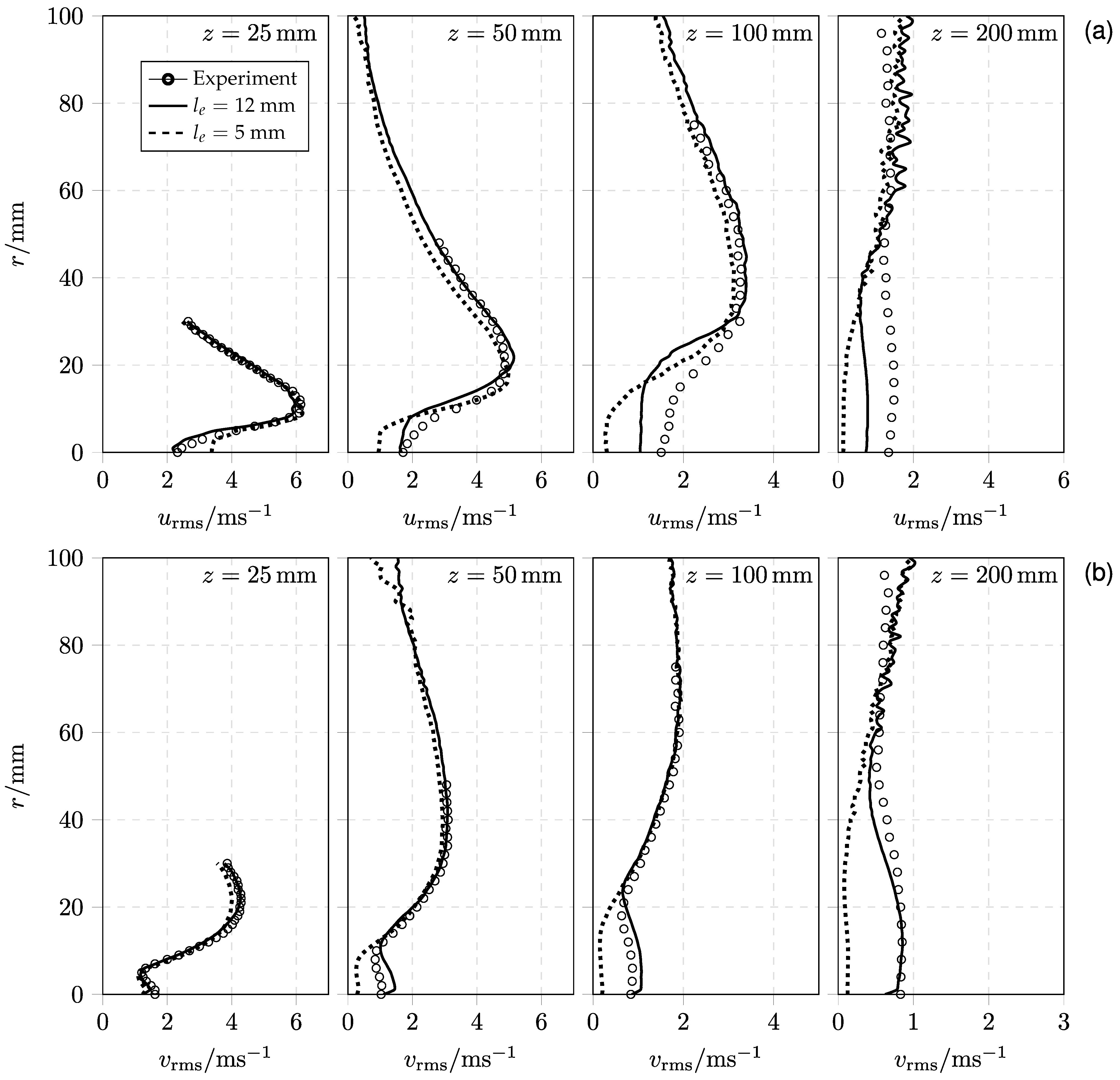
In the following section, the results obtained from the numerical simulations are presented. First, neglecting droplet–droplet collisions, the results for the two injection methods, Case 1a and Case 2a, are discussed in detail and compared with the experimental data. Subsequently, the influence of different collision-regime maps is analyzed.

3.1. Comparison of the Injection Models

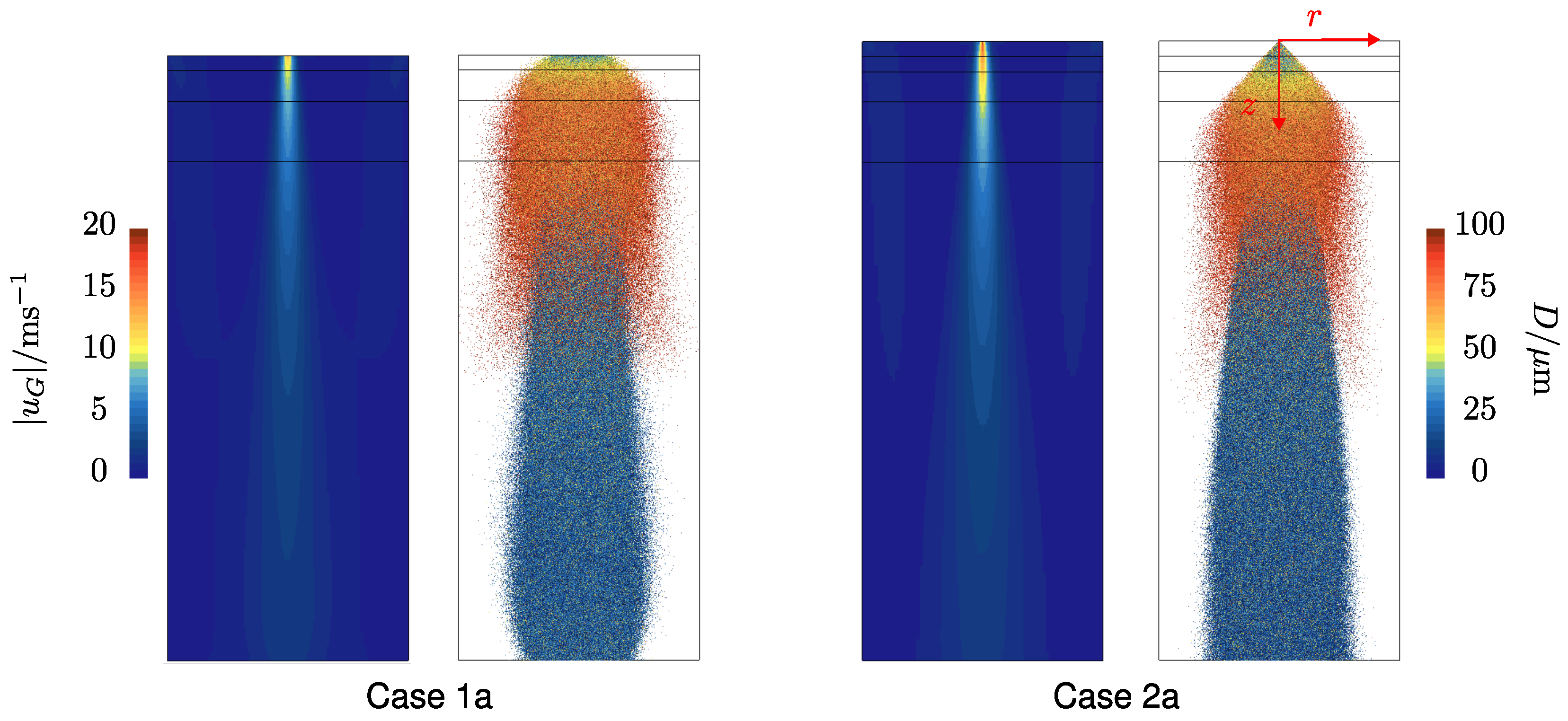
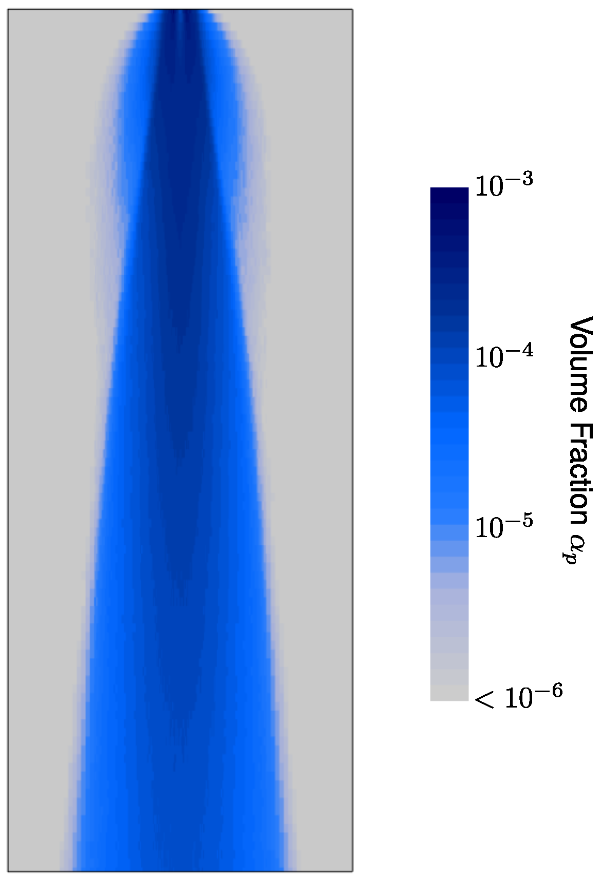
To compare the two injection methods described in Section 2.2.1, the instantaneous fields of gas velocity magnitude and droplet diameter at $t=0.5\mathrm{s}$ are shown in Figure 6. For both cases, the airflow is accelerated due to droplet injection and the applied two-way coupling approach. Because of the resulting steep velocity gradients, the mesh is locally refined in the core region of the spray. In Case 2a, where the droplet injection is located further upstream ($z=0\mathrm{m}$), higher gas velocities are observed near the injection region compared with Case 1a. This is attributed to the larger injection velocity of the droplets, calculated from Equation (4). Since no airflow measurements are available in this region, the experimental data from the first measurement section ($z=25\mathrm{mm}$) were projected as the upper-boundary condition of the cylinder, which may introduce a potential source of uncertainty in the solid-cone injector model. In addition to the gas velocity, the droplet diameters are visualized for both cases in Figure 6. To better highlight the relevant size range, only droplets with diameters up to $D=100$ μm are shown. Both cases exhibit qualitatively similar spray behavior, with smaller droplets concentrated in the core region and larger droplets distributed toward the periphery. Due to the outward spreading of the spray, a small number of large droplets impinge onto the cylinder wall and are removed from the domain. As discussed previously, preliminary simulations indicate that droplet–wall interactions have a negligible influence on the mean droplet properties. Therefore, they are neglected in all subsequent analyses. Furthermore, the spray in Case 2a shows a slightly reduced radial spread, particularly in the upper region. This difference may be attributed to the specified spray angle and the trigonometric assumption used to define the injection velocity vector.

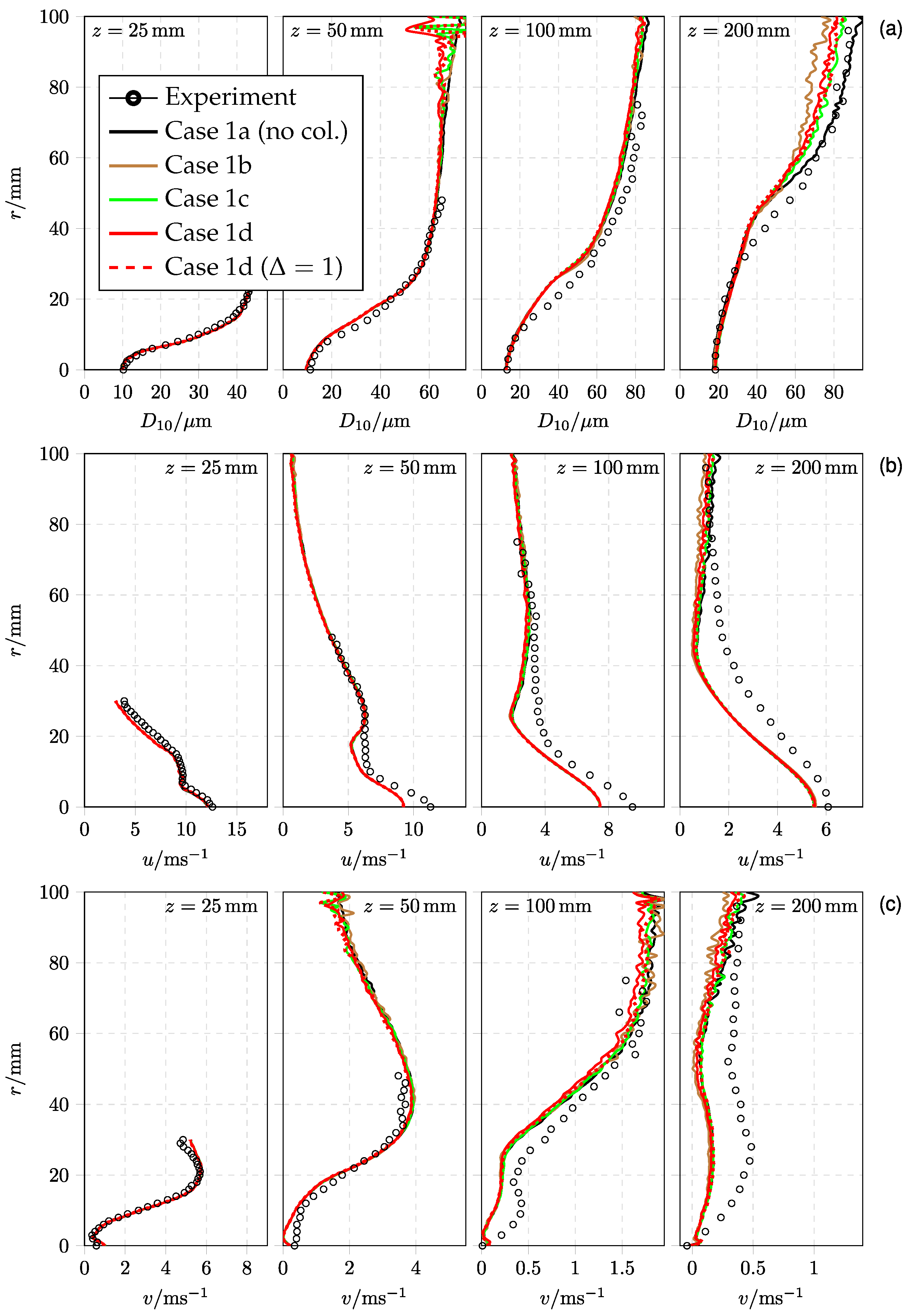
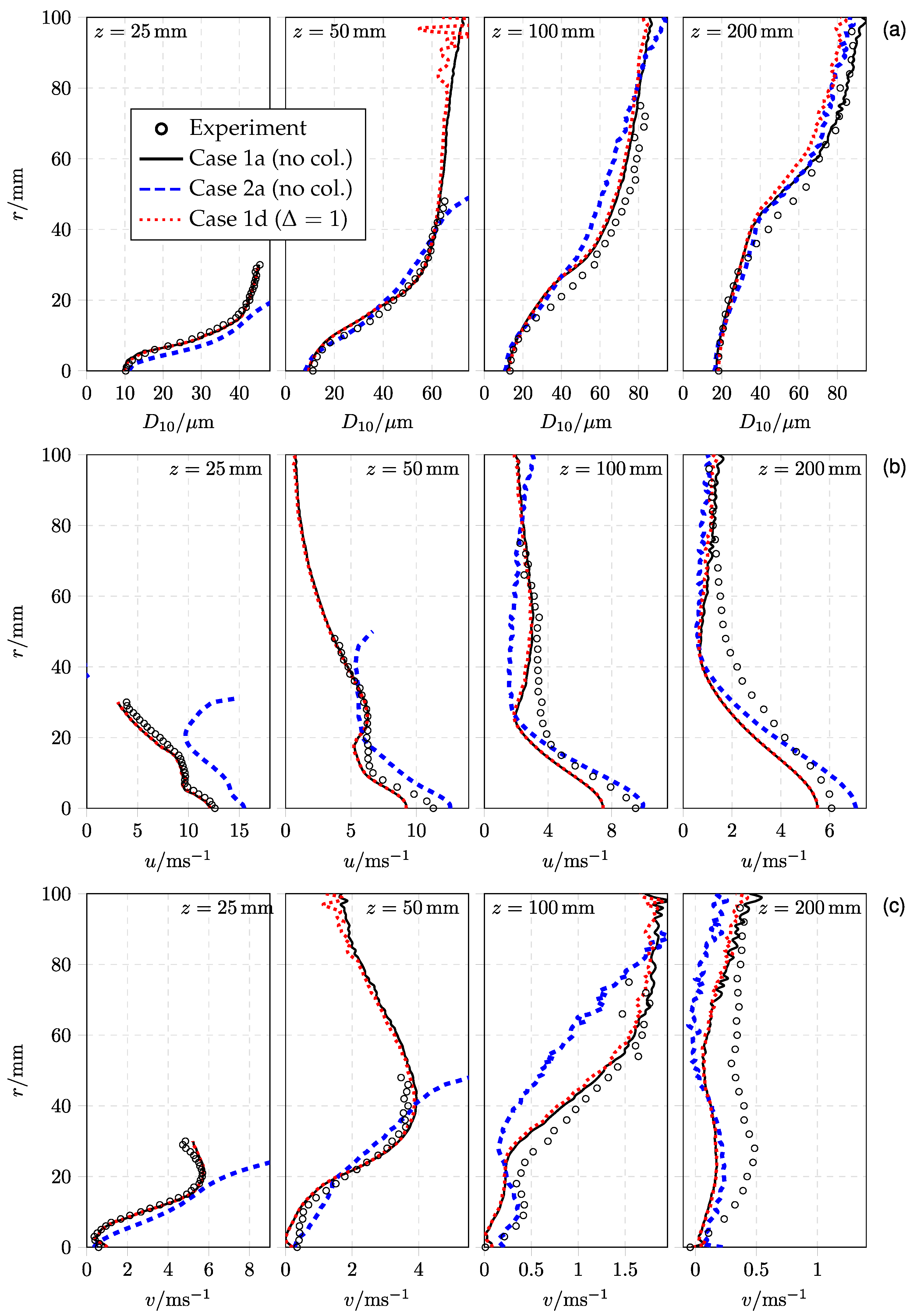
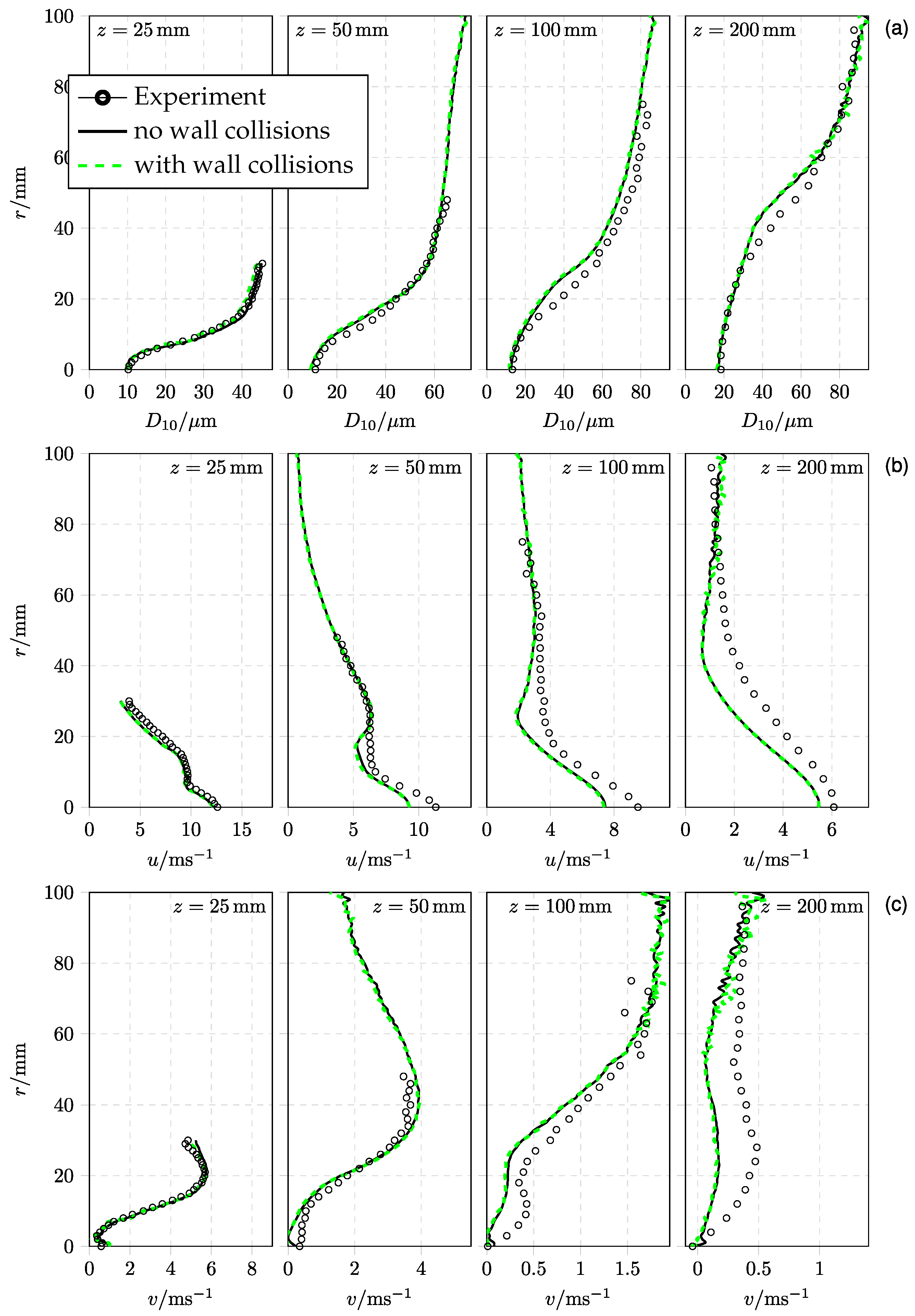
Following this qualitative comparison of the overall spray structure, a quantitative analysis of the droplet statistics is conducted. Figure 7 presents the radial distributions of the droplet number-mean diameter ($D_{10}$) and the velocity components ($u,v$) at the four measurement sections. The numerical results are compared with experimental data for the array of injectors (Case 1a) and the solid-cone injector (Case 2a). In addition, one representative collision case (Case 1d, fixed $\Delta$) is included to illustrate the potential influence of droplet–droplet collisions and is discussed in detail in Section 3.2. Both simulations that neglect droplet collisions show overall good agreement with the experiments, particularly for the droplet diameter (see Figure 7a). Due to the transport by the entrained airflow, smaller droplets tend to accumulate near the spray centerline and exhibit higher velocities. In contrast, larger droplets originate from the breakup of the conical liquid film, follow the direction of the liquid cone, and are predominantly located at the spray periphery. Compared with the results of Lain and Sommerfeld [2], the droplet diameters in the measurement sections at $z=100\mathrm{mm}$ and $z=200\mathrm{mm}$ are not overpredicted but instead slightly underpredicted. The predicted radial spread of the spray (Figure 7c) also appears to be marginally smaller than in the measurements, which consequently affects the droplet number-mean diameter, as also observed by Lain and Sommerfeld [2]. For the droplet velocities, some larger deviations between simulation and experiment are observed further downstream. 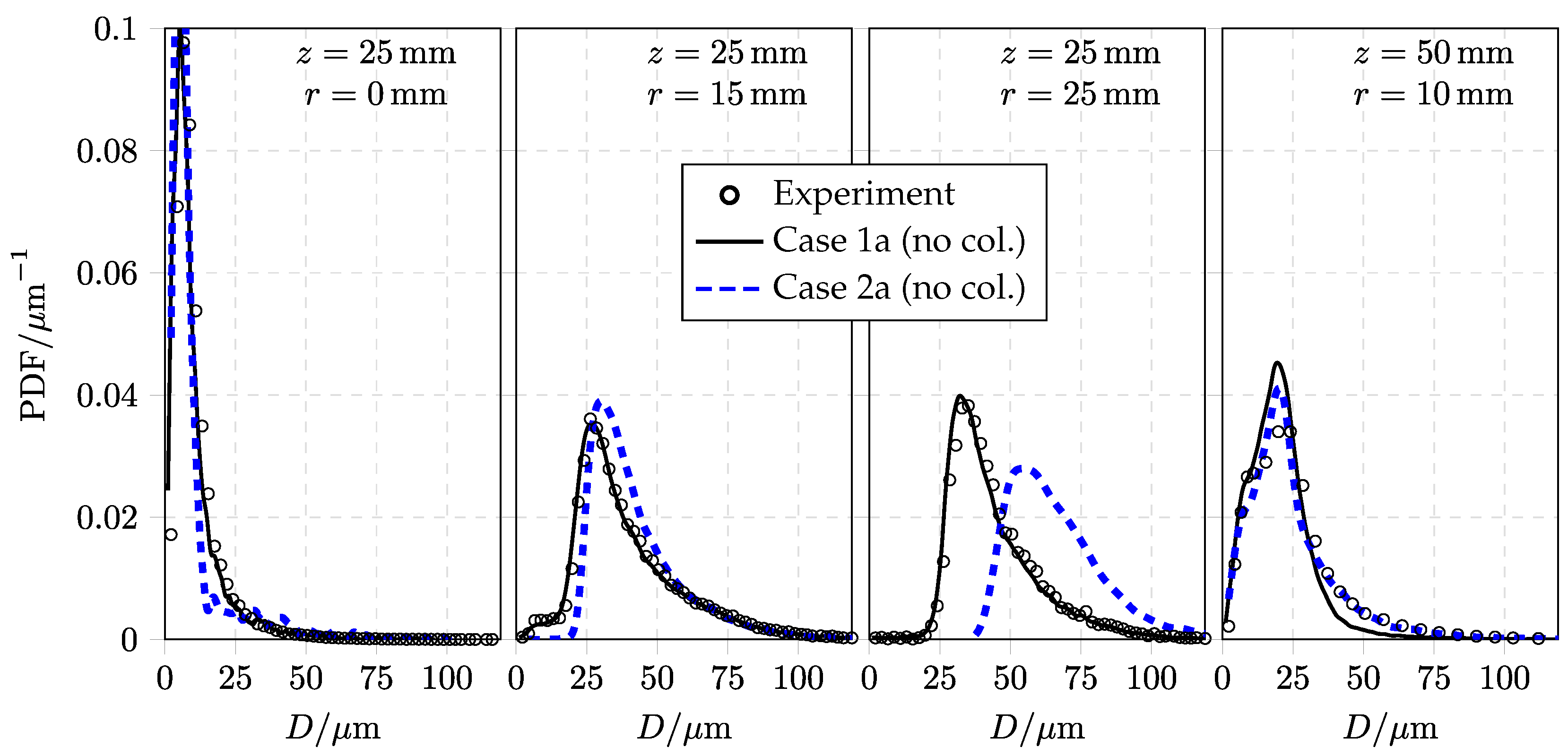Furthermore, Figure 8 compares three measured number-based size distributions (PDFs) at different locations with numerical predictions. For Case 2a, the distributions in the core region of the first measurement section (e.g., $z=25\mathrm{mm}$, $r=0\mathrm{mm}$, and $z=25\mathrm{mm}$, $r=15\mathrm{mm}$) show good agreement with the experimental data. However, larger differences are observed in the outer region of the first measurement section (e.g., $z=25\mathrm{mm}$, $r=25\mathrm{mm}$). These deviations in the outer region are also reflected in the droplet number-mean diameter shown in Figure 7a. The distributions from Case 1a align perfectly with the experiments in the first measurement section, as this section represents the boundary condition for droplet introduction. Additionally, the local PDF is compared at another location further downstream of the spray nozzle ($z=50\mathrm{mm}$, $r=10\mathrm{mm}$), where both simulation models accurately predict the measured distribution shape. Case 2a appears to predict the absolute PDF-values for larger diameters slightly better. To quantify the overall differences in each measurement section between simulations and experiments, the mean absolute error ($\mathrm{MAE}$) and the mean relative error ($\mathrm{MRE}$) of a parameter X (e.g., droplet diameter) are calculated as given by Equation (7). The results are presented in

Table 4. Mean absolute error ($\mathrm{MAE}$) and mean relative error ($\mathrm{MRE}$) between numerical and experimental data at different z-positions and for Case 1a and Case 2a.

	$\mathbf{MAE}\left(\mathbf{MRE}\right)$	$\mathit{z}=25\mathbf{mm}$	$\mathit{z}=50\mathbf{mm}$	$\mathit{z}=100\mathbf{mm}$	$\mathit{z}=200\mathbf{mm}$
	$D_{10}/\mathsf{\mu }\mathrm{m}$	$0.7(3\%)$	$1.7(6\%)$	$4.6(9\%)$	$2.8(6\%)$
Case 1a	$u/{\mathrm{ms}}^{-1}$	$0.6(8\%)$	$0.5(6\%)$	$0.8(18\%)$	$0.7(31\%)$
	$v/{\mathrm{ms}}^{-1}$	$0.2(8\%)$	$0.2(22\%)$	$0.2(54\%)$	$0.2(52\%)$
	$D_{10}/\mathsf{\mu }\mathrm{m}$	$12.7(35\%)$	$2.5(7\%)$	$8.6(15\%)$	$4.5(8\%)$
Case 2a	$u/{\mathrm{ms}}^{-1}$	$3.8(59\%)$	$1.0(17\%)$	$1.1(31\%)$	$0.7(35\%)$
	$v/{\mathrm{ms}}^{-1}$	$2.2(73\%)$	$0.4(27\%)$	$0.4(114\%)$	$0.3(91\%)$

.

$$\mathrm{MAE}={\displaystyle \frac{1}{N}}{\displaystyle \sum _{i=1}^N}|X_{i,\mathrm{sim}}-X_{i,\exp }|\mathrm{MRE}={\displaystyle \frac{1}{N}}{\displaystyle \sum _{i=1}^N}\left|{\displaystyle \frac{X_{i,\mathrm{sim}}-X_{i,\exp }}{X_{i,\exp }}}\right|·100$$

(7)

Case 1a: Since, in Case 1a, the droplets are introduced at the measurement section at $z=25\mathrm{mm}$, only small differences from the measurements are observed due to the post-processing method. In this section, the droplet number-mean diameter deviates by $0.7$ μm from the experiments, with a relative mean error of $3\%$ (see Table 4). The deviations in droplet diameters are slightly larger in the other measurement sections, with a maximum difference of $4.6$ μm ($9\%$). Even though the profile shapes of the axial and radial velocities are well-predicted, larger differences are quantified. While the mean absolute error for the velocities remains below $1\mathrm{m}/\mathrm{s}$, higher mean relative errors are observed. This is due to the relatively small values in the denominator of the $\mathrm{MRE}$ equation (Equation (7)), which result in higher $\mathrm{MRE}$ values for the radial velocities compared to the axial velocities. However, measuring velocities with PDA can be challenging, and, therefore, the mean absolute deviations below $1\mathrm{m}/\mathrm{s}$ are within an acceptable range.

Case 2a: Here, larger differences are observed in the first measurement section compared to Case 1a. In contrast to Case 1, the droplets are now introduced at $z=0\mathrm{mm}$ with properties from the measurement section at $z=25\mathrm{mm}$, because no measurement data exist upstream of this section. PDA measurements in this region are not recommended, as primary breakup of the spray is not yet completed. Hence, for Case 2a, larger deviations are expected in the first measurement section due to the lack of data needed to specify the boundary conditions more accurately. This deviation is likely a consequence of the missing correlation between injected droplet diameter and velocity. Another possible reason is that primary breakup is not modeled in this work. However, Case 2a performs well in the other measurement sections, achieving similar accuracy as Case 1a (see Table 4). Disregarding the errors in the first measurement section, the maximum $\mathrm{MAE}$ for the diameters across all sections is $8.6$ μm ($15\%$). Compared to Case 1a, the velocities in the core region of the spray match better with the measurements. Similarly, comparable $\mathrm{MAE}$ values (≤1 m/s) are observed, while higher $\mathrm{MRE}$ values are visible.

3.2. Influence of Collisions

In this section, droplet–droplet collisions are investigated using three additional cases (Case 1b, Case 1c, and Case 1d), as summarized in Table 3. The injection setup from Case 1a is retained, while three different collision-regime maps available in STAR-CCM+ are applied. The aim is to assess the influence of the collision models, and in particular the droplet size ratio $\Delta$, on the predicted collision outcomes and resulting spray characteristics.

Table 5. Collision statistics for different collision outcome maps.

Case	Collisions	Bouncing/%	Coalescence/%	Stretching/%	Reflexive/%
Case 1b	$9.64\times {10}^7$	99.9	0.10	0.00	0.00
Case 1c	$8.11\times {10}^7$	-	99.9	0.10	0.00
Case 1d	$9.45\times {10}^7$	92.5	7.35	0.15	-

summarizes the total number of detected collisions and the relative contribution of the individual collision outcomes for the different collision maps. A pronounced dependence on the selected collision map can be observed. The Composite map (Case 1b) predicts an almost complete dominance of bouncing, with negligible contributions from other regimes. In contrast, the Ashgriz-based model (Case 1c) yields predominantly coalescence, as the model formulation does not include a distinct bouncing regime. The O’Rourke map (Case 1d) shows an intermediate behavior, with bouncing still dominating but with a noticeable contribution from coalescence. As shown in Table 5, reflexive and stretching separation contribute only marginally and are negligible for all investigated cases.

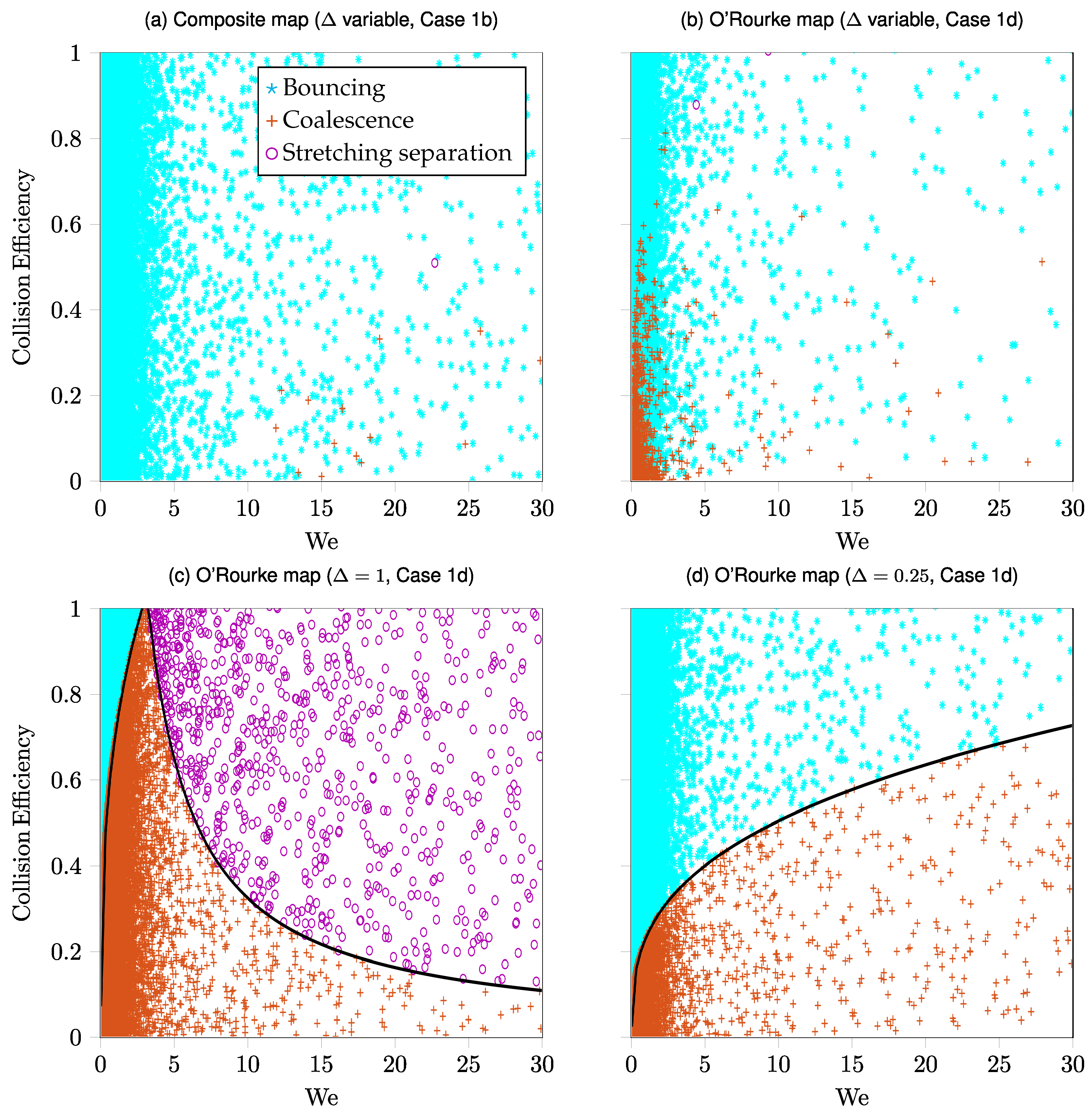
This behavior can be further understood by analyzing the underlying collision-regime maps together with the simulated collision outcomes. Most collisions occur in the near-field region, where droplet number densities are highest, providing the basis for the subsequent analysis of collision outcomes. Figure 9a,b show the collision efficiency over the relative Weber number for the Composite (Case 1b) and O’Rourke (Case 1d) maps with variable $\Delta$, including the simulated collision outcomes. It can be observed that the majority of collisions occur at relatively low Weber numbers ($We\lesssim 5$). In this regime, the dominant collision outcomes are bouncing and coalescence, with only a minor contribution from stretching separation. For variable $\Delta$, both models predict a pronounced dominance of bouncing, particularly for the Composite model, see also Table 5.

To further illustrate the influence of $\Delta$, Figure 9c,d show the O’Rourke map for fixed values of $\Delta$. A strong dependence of the bouncing boundary on the droplet size ratio $\Delta$ can be observed. For $\Delta =1$, the bouncing regime is significantly reduced, leading to an increased contribution of coalescence and stretching separation. For $\Delta =0.25$, the bouncing boundary is shifted towards higher Weber numbers, which significantly enlarges the bouncing regime.

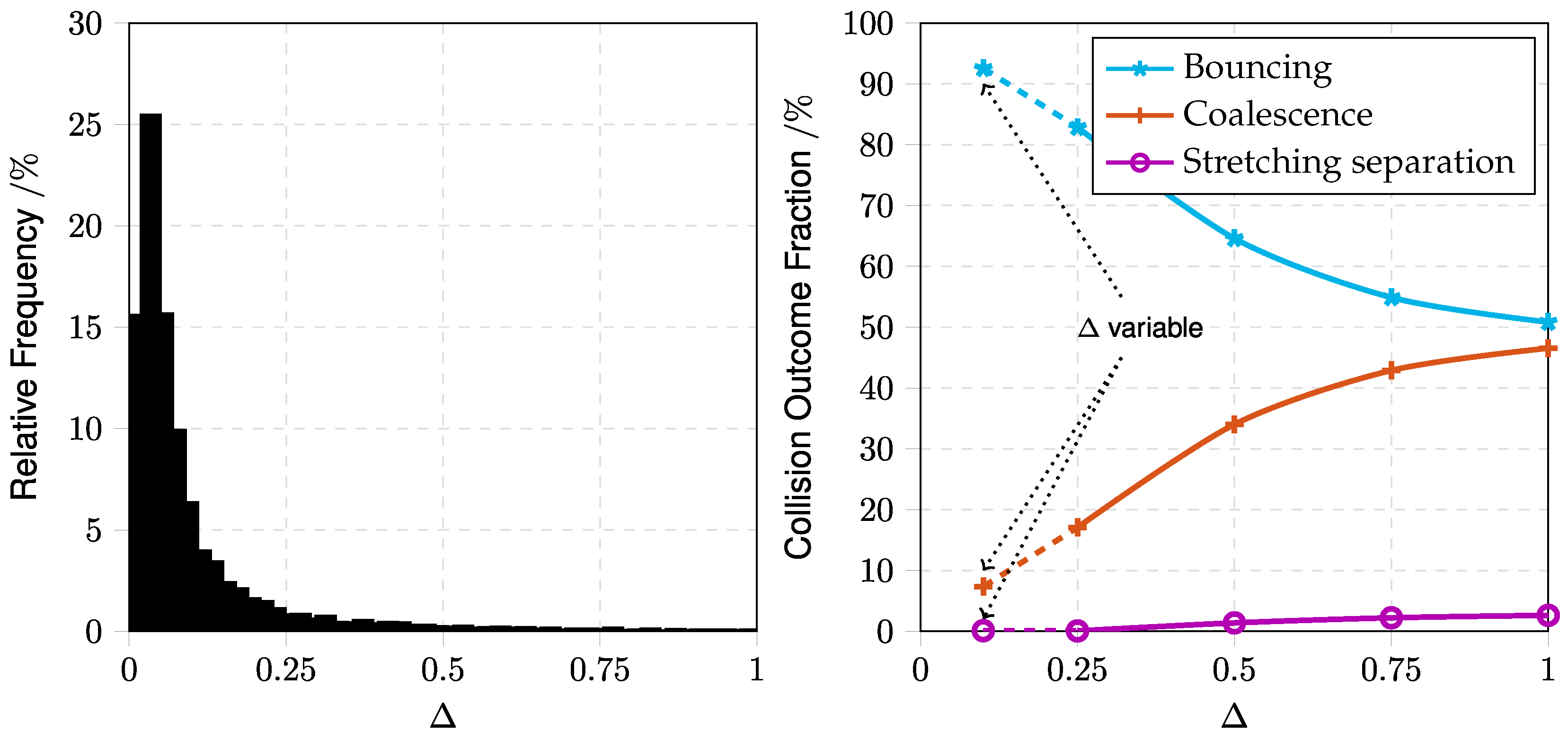
This pronounced sensitivity of the collision outcome to the droplet size ratio $\Delta$ is further quantified in Figure 10. Figure 10 shows the distribution of $\Delta$ for the investigated spray. The majority of collisions occur at small droplet size ratios $\Delta$, indicating that interactions between droplets of dissimilar sizes dominate the collision process. Figure 10b quantifies the influence of $\Delta$ on the collision outcome using the O’Rourke map. Decreasing $\Delta$ leads to a strong increase in the bouncing fraction, while coalescence is progressively suppressed. For $\Delta \approx 1$, the behavior is more balanced, whereas for smaller values, bouncing becomes dominant. The result obtained for the variable-$\Delta$ case (indicated in Figure 10b) closely follows the behavior at small $\Delta$, consistent with the distribution shown in Figure 10a. This can be explained by the functional dependence of the collision boundaries on $\Delta$ (see Appendix D). As $\Delta$ decreases, the boundary shifts towards higher Weber numbers, increasing the likelihood of bouncing. This indicates that the predicted collision behavior in the investigated polydisperse sprays is largely governed by interactions at small droplet size ratios $\Delta$, which dominate the overall collision frequency. 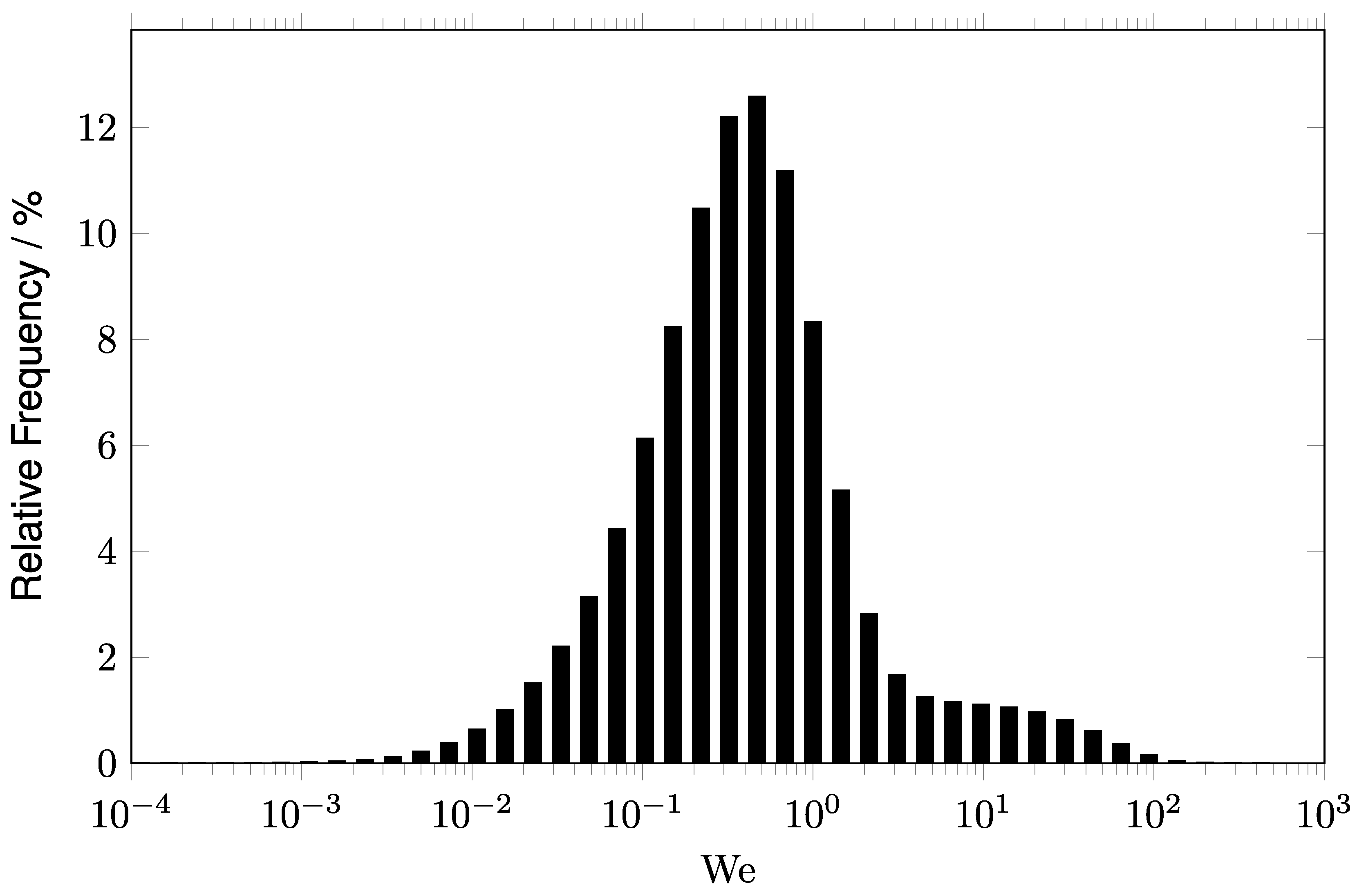To further quantify the collision conditions, Figure 11 shows the relative frequency distribution of the collision Weber number for the O’Rourke map within the validation region $z\le 200\mathrm{mm}$. The distribution is shown on a logarithmic Weber number scale and confirms that most detected collision events occur at relatively low Weber numbers, with the highest frequencies occurring below $We=1$. Collisions at higher Weber numbers are considerably less frequent, and most events remain below approximately $We\le 5$. Consequently, many collisions are low-energy events that mainly affect droplet trajectories, while high-energy collision events remain comparatively rare, which is also consistent with the negligible contribution of separation regimes.

Despite the pronounced differences in collision outcomes and their strong dependence on the droplet size ratio $\Delta$, it remains unclear to what extent these variations affect the resulting spray characteristics. To quantify this, the cross-sectional averages of the droplet number-mean diameter $D_{10,A}$ and the Sauter mean diameter $D_{32,A}$ are evaluated. The Sauter mean diameter represents the ratio of droplet volume to surface area and is a key parameter for heat and mass transfer in two-phase flows. The cross-sectional average of a general droplet diameter $D_{ij}$ is defined as

$$D_{ij,A}={\displaystyle \frac{{\sum }_k{A}_k{D}_{ij,k}}{{\sum }_k{A}_k}},$$

(8)

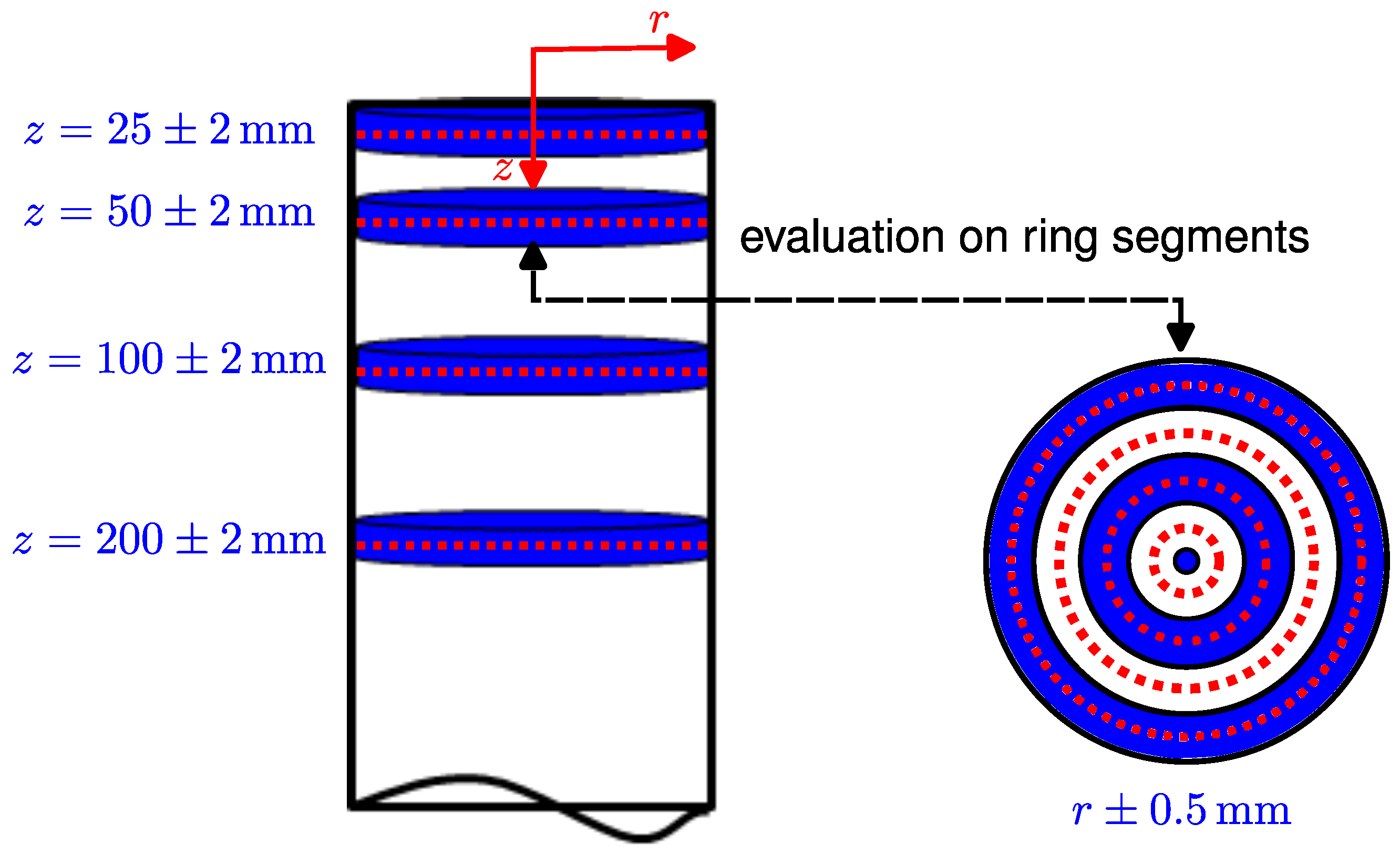
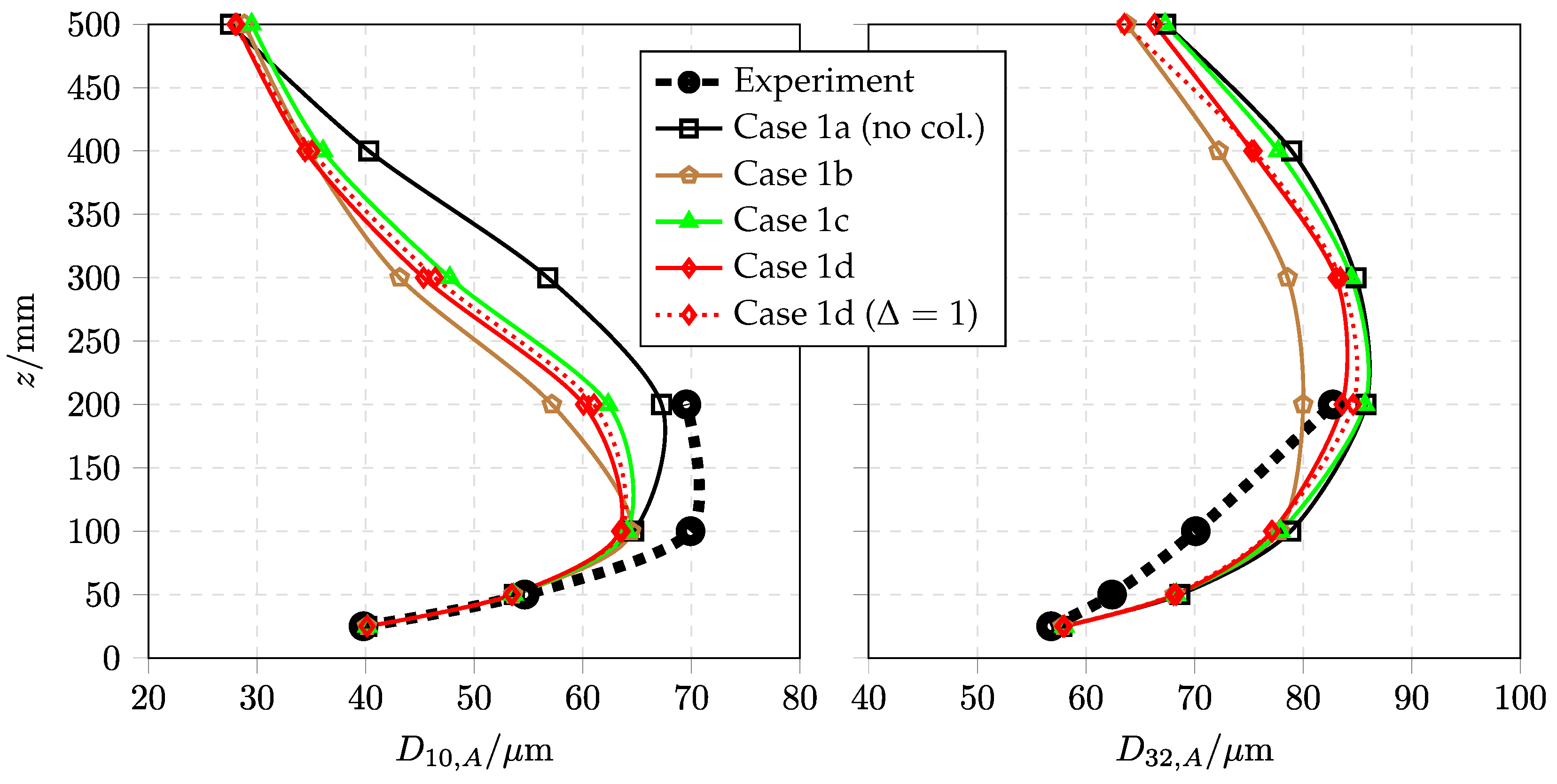
where $D_{ij,k}$ is evaluated in the k-th radial ring with corresponding area $A_k$ (see Figure 5). For consistency with the experiments, the averaging is restricted to the measured radial range. Figure 12 shows the axial evolution of both diameters for the different collision models, including a reference case without collisions and one case with fixed $\Delta =1$. The experimental data reveal that both quantities increase with downstream distance, with $D_{10,A}$ reaching its maximum at $z=100\mathrm{mm}$. The simulations reproduce this general trend, although deviations in both magnitude and axial location of the maximum are observed. While the agreement is good in the near-field ($z\le 50\mathrm{mm}$), increasing deviations occur further downstream. In this region, the droplet size evolution is strongly influenced by upstream collision processes, which are treated differently by the individual collision maps. Case 1b predicts consistently smaller values of both $D_{10,A}$ and $D_{32,A}$, which can be attributed to the strong dominance of bouncing and the associated redistribution of droplet momentum in the downstream region. Consistent with this behavior, the liquid mass removed at the wall in the downstream region ($200<z<1000\mathrm{mm}$) increases from approximately $1\%$ without collisions to approximately $2.6\%$ for the investigated collision cases. Within the validation region ($z\le 200\mathrm{mm}$), however, the liquid mass removed at the wall remains below $0.01\%$ of the injected liquid mass. In contrast, the Ashgriz-based model (Case 1c) shows good agreement with the no-collision case for $D_{32,A}$, indicating a limited impact of coalescence-dominated behavior on near-field spray characteristics, see also Figure A4. For the O’Rourke model (Case 1d), only minor differences are observed between variable and fixed $\Delta$, despite significant differences in the collision outcomes. This behavior is consistent with the local droplet distributions shown in Figure 7. Although the collision maps lead to markedly different event-based collision outcomes, the collision statistics in Table 5 represent outcome fractions among detected collision events and therefore do not directly quantify the influence on the entire droplet population. In addition, the distributions of droplet size ratios (Figure 10a) and collision Weber numbers (Figure 11) indicate that most collisions occur at small $\Delta$, and at comparatively low collision Weber numbers. For bouncing events, this mainly results in a redistribution of droplet momentum without modifying the droplet size. For coalescence events involving small $\Delta$, the resulting increase in the larger droplet diameter remains moderate because the volume contribution of the smaller droplet is comparatively small. Local differences between the collision models are nevertheless visible in the radial profiles, particularly in the downstream region (see Appendix E). The largest local differences between the investigated collision maps are observed for Case 1b in the downstream droplet-size profile at $z=200\mathrm{mm}$, where local deviations of up to approximately $24\%$ relative to the no-collision case (Case 1a) occur. In contrast, at the same axial location, the corresponding cross-sectional averaged droplet diameters differ by only $15.2\%$ for $D_{10,A}$ and $7.7\%$ for $D_{32,A}$. For example, coalescence-dominated and bouncing-dominated cases modify the radial droplet-size profiles differently. However, these local variations are partly smoothed when cross-sectional averaged quantities such as $D_{10,A}$ and $D_{32,A}$ are evaluated. This explains why the cross-sectional averaged quantities show a weaker sensitivity to the collision map than the local radial profiles. It should also be noted that the applied collision-mesh approach in STAR-CCM+ performs collision detection within dynamically reconstructed collision volumes based on parcel statistics and estimated particle mean free paths. Therefore, the collision detection is not strictly local on the CFD cell level, which may also contribute to smoothing effects in the local collision statistics.

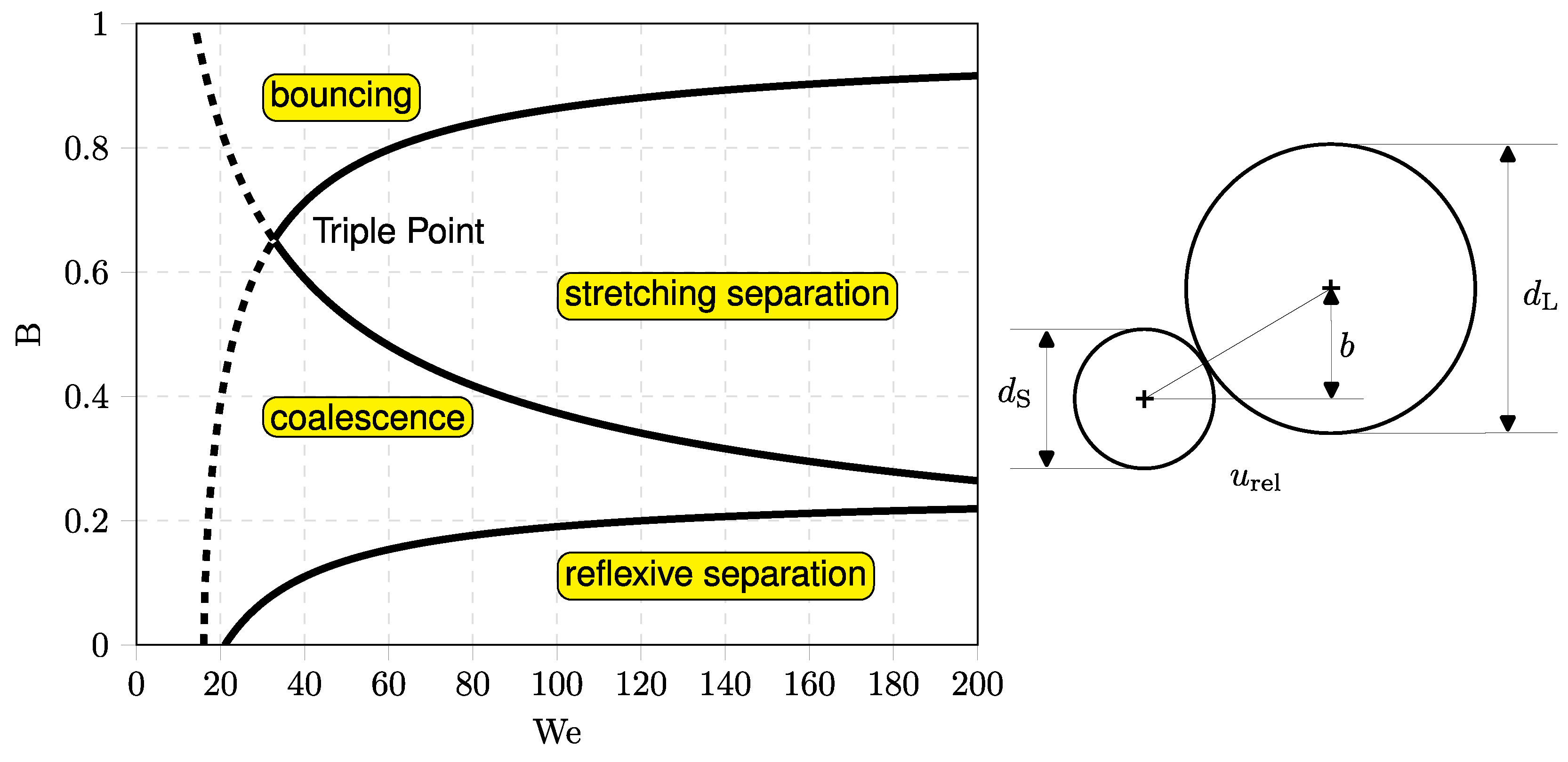
In addition to the dependence on $\Delta$, the formulation of the bouncing boundary plays a critical role. In STAR-CCM+, bouncing is allowed down to head-on collisions ($\mathrm{B}=0$), as indicated by the dashed line in Figure 4. This leads to reduced coalescence rates in Cases 1b and 1d. In the literature (e.g., [2]), the bouncing boundary is often truncated at the triple point (see Figure 4), so that bouncing is only considered at higher $\mathrm{B}$ values, where the droplets barely graze each other. Such a situation is experimentally found for water droplets as summarized by Sui et al. [36]. Furthermore, the impact efficiency, which is not considered in the present work, may reduce collision frequencies in polydisperse sprays. This parameter is especially relevant for interactions between droplets of very different sizes, where smaller droplets may follow the gas streamlines around larger ones instead of colliding [2].

4. Conclusions

The present study investigates the water spray behavior through numerical simulations, focusing on validating computational models against the experimental data of Rüger et al. [17], who measured droplet size and velocity distributions in four downstream sections of a spray nozzle. The results show that smaller droplets concentrate in the spray core and exhibit higher velocities, while larger droplets are found at the periphery as a result of inertia and hollow-cone liquid sheet breakup. Two injection modeling strategies are evaluated using the Euler/Lagrange approach in STAR-CCM+: an injector array (Case 1) and a solid-cone injector model (Case 2). Both approaches capture the essential spray characteristics, particularly the radial profiles of the droplet number-mean diameters and the number-based local particle size distributions (PDFs) in the first two measurement sections agree well with the experiments. The radial spread of the spray is slightly underpredicted in both cases, which consequently affects the downstream droplet size predictions. Velocity comparisons indicate good overall agreement, although larger deviations occur further downstream, likely due to cumulative modeling uncertainties such as in the treatment of turbulent dispersion.

Case 1, which introduces droplets based on locally measured size distributions and velocity profiles, provides the closest agreement with the experimental data for the radial velocity distributions. This improvement can be attributed to the more accurate representation of the injection conditions, leading to a more realistic spray evolution. In contrast, the simple solid-cone injector model (Case 2), while more practical, shows larger discrepancies in the first measurement section due to the absence of a direct experimental input upstream of $z=25\mathrm{mm}$. This deviation likely results from the missing correlation between the injected droplet diameter and velocity. The error analysis, based on the mean absolute error ($\mathrm{MAE}$) and the mean relative error ($\mathrm{MRE}$), quantifies these deviations and confirms that Case 1 consistently exhibits smaller error margins compared with Case 2. Nevertheless, the solid-cone injector model (Case 2) remains a viable alternative when computational efficiency is prioritized or when only limited measurement data are available, provided that its limitations are recognized. It should be noted that the solid-cone injector employs a uniform angular sampling of the injected droplets and therefore does not fully reproduce the hollow-cone spray structure of the investigated nozzle. Consequently, the model should be regarded as a practical simplified injection approach rather than a physically accurate representation of the nozzle atomization process.

Beyond the injection modeling, the influence of droplet–droplet collision models on the spray development is also examined. The results demonstrate that different collision-regime maps lead to substantially different event-based collision outcomes, with a strong sensitivity to the droplet size ratio $\Delta$. In particular, the extent of the bouncing regime is significantly affected by both the collision model and the treatment of $\Delta$. Despite these pronounced differences in collision behavior, the cross-sectional averaged spray quantities show only limited sensitivity to the selected collision model. This is mainly attributed to the fact that most collision events occur at comparatively low collision Weber numbers and small droplet size ratios, such that many collisions remain low-energy events that primarily affect droplet trajectories rather than causing strong changes in integral spray quantities. Nevertheless, local differences between the collision models remain visible in the downstream radial spray profiles, particularly for the droplet diameter distributions.

Overall, this study highlights the importance of accurate injection modeling for spray simulations, while providing insight into the role and limitations of collision modeling in polydisperse sprays. The formulation of the bouncing boundary and additional effects such as impact efficiency remain important aspects for improving the physical consistency of collision modeling in polydisperse sprays and should be addressed in future work.