Article

Rapid Prediction of Leakage Dispersion at Natural Gas Distribution Stations: A Prototype Development Using Computational Fluid Dynamics and Machine Learning

1
College of Safety Engineering, Chongqing University of Science and Technology, Chongqing 401331, China
2
School of Chemical Engineering, Oklahoma State University, Stillwater, OK 74078, USA
3
College of Chemistry and Chemical Engineering, Southwest Petroleum University, Chengdu 610500, China
4
School of Environmental Science and Safety Engineering, Tianjin University of Technology, Tianjin 300384, China
5
Southwest Oil and Gas Field Branch of China National Petroleum Corporation, Chengdu 610500, China
*
Authors to whom correspondence should be addressed.
Fluids 2026, 11(6), 137; https://doi.org/10.3390/fluids11060137
Submission received: 25 April 2026 / Revised: 27 May 2026 / Accepted: 28 May 2026 / Published: 31 May 2026
(This article belongs to the Special Issue 10th Anniversary of Fluids—Recent Advances in Fluid Mechanics)

Abstract

Leakage incidents at natural gas distribution stations (NGDSs) present severe fire and explosion risks, demanding immediate, data-driven emergency responses. While crucial for minimizing hazard impacts, real-time prediction of gas dispersion ranges remains a significant operational challenge. To partially address this critical safety need, this study introduces a rapid-response prediction framework prototype integrating computational fluid dynamics (CFD) with machine learning (ML). Specifically, a comprehensive database of 500 experimentally validated CFD leakage scenarios at 60 s was developed first, specifically focusing on mapping gas concentration contours within the critical 5–15% flammability range. To identify the most effective real-time predictive tool, three ML algorithms, including a backpropagation neural network (BPNN), long short-term memory (LSTM), and gated recurrent unit (GRU), were evaluated. The BPNN initially outperformed the sequence models, with a coefficient of determination (R2) of 0.96, a mean squared error (MSE) of 1.35, a mean absolute error (MAE) of 0.77, a maximum absolute error (MaxAE) of 4.94 and an average training time of 4.23 s per epoch. To further meet the stringent speed and precision demands of emergency scenarios, the model was enhanced via particle swarm optimization (PSO-BPNN). This optimized framework achieved exceptional accuracy (R2 = 0.99, MSE = 0.34, and MAE = 0.38) while reducing the training time to just 1.42 s per epoch under the current computational configuration. The developed CFD-ML prototype provides a practical, highly efficient tool for NGDS operators and emergency responders, enabling them to instantly visualize hazard zones, optimize evacuation protocols, and safely mitigate leakage incidents before ignition occurs.

1. Introduction

A natural gas distribution station (NGDS) is a pivotal transition network from end to end in regulating and distributing natural gas. During daily operation in an NGDS, accidental leakages could happen, possibly leading to severe consequences, such as fires and explosions, if proper emergency responses are not carried out [1,2,3,4,5]. Practically, in industrial applications, it is impossible to avoid all accidental leakages in NGDSs due to not only the fact that the distribution system is the spatially largest and most complex part of the entire natural gas supply chain, but also that direct comprehensive observation of the emissions from these systems is logistically challenging [6]. A prompt emergency response is essential to minimize losses caused by a leakage accident. To act efficiently, emergency responders require accurate and reliable information regarding the exact location of the leak and its potential dispersion range.
In general, there are three pathways to secure the dispersion range of natural gas in NGDSs, i.e., field and wind tunnel experiments, empirical models, and computational fluid dynamics (CFD) [7,8,9,10,11,12,13]. To date, only limited field experiments have been conducted to investigate natural gas dispersion scenarios with the associated critical parameters (i.e., evaporation rate, pool-spreading speed, and dispersion range) [14,15], which have been used as the fundamental data for proposing empirical models. However, due to the disadvantages of long periods, high costs, the randomness of environmental conditions and low reproducibility in the field experiments [11], such experiments have rarely been conducted in the past 30 years. To overcome these drawbacks, wind tunnel experiments have become an alternative, avoiding large-scale field experiments and ensuring that the whole test process is more controllable. Based on experimental results, some empirical models and CFD models have been proposed to investigate the dispersion properties (i.e., gas concentration, the shape of the cloud plume, vortex size and locations) of natural gases affected by wind direction and magnitude, ground obstacles, orifice size and shape, leakage rate and pressure, etc. [12,16,17,18,19]. According to the state of leakage sources, empirical leakage models can be divided into instantaneous and continuous leakage models [20], and the leakage scenarios at NGDSs are categorized into the latter one. Two representative dispersion models, i.e., the Britter–McQuaid model (also called the phenomenological model and nomogram model) [21] and the integral model (e.g., HEGADAS [22], DEGADIS [23], and SLAB [24]), have been widely used to estimate some common characteristics of gas clouds, such as the average cloud radius, the average cloud height and the average cloud temperatures. These results have been utilized as references for emergency counselling and responses. However, these empirical models cannot fit all natural gas dispersion scenarios, and the estimation accuracy is highly dependent on fundamental experimental data and appropriate parametric setups, such as safe dispersion coefficients, gas pressure drop and kinetic energy changes [8,25].
Compared with empirical models, CFD modeling has unique features that include complicated obstacles and terrains in the computational domains, which can mimic realistic flow fields and diffusion fields at an NGDS [26,27,28]. Shen et al. [13] also summarized that the primary advantage of CFD simulation models lies in their ability to account for complex interactions between obstructions and fluid flow, which is especially important when a flammable gas disperses in geometrically complex environments, such as urban areas, chemical plants, and NGDSs. This capability enables the real-time estimation of flammable material dispersion even in intricate geometric settings. The stability and accuracy of CFD modeling depend on the agreement with experimental tests, which varies with the employed turbulence models and has intensive requirements for a fundamental understanding of the mathematical calculations. Moreover, its computational efficiency depends on the number of computational mesh cells and the equipped computing sources, limiting its application in instant emergency responses once accidental leakages happen [29]; therefore, a more effective and prompt alternative is urgently needed.
Driven by the rapid development of artificial intelligence (AI) applications in fire protection and process safety engineering [30,31,32,33,34,35,36], it has become possible to find an alternative pathway to help emergency responders obtain real-time natural gas dispersion range in NGDSs precisely based on the leakage conditions by directly using machine learning (ML) algorithms, without the need for complicated CFD knowledge in emergency responders, which is, currently, the most popular method to predict gas dispersion scenarios while being time-consuming and quite complex in the computing process [36,37,38,39]. A recent review by Jiao et al. [40] highlighted that implementing machine learning surrogate models in process safety research can significantly save human, material, and financial resources, owing to their unparalleled advantages in trend identification and predictive assistance. An appropriate ML algorithm with training and testing stages can deliver decent predictions in natural gas dispersion, while the biggest challenge is how to incorporate all dispersion scenarios into the ML framework, which needs a solid database to train ML algorithms [29,40]. The natural gas dispersion parameters (i.e., wind speed and direction, leakage pressure and direction, and aperture size) in NGDSs have a close relationship with the dispersion scenarios, such as the dispersion range and gas concentration, leading to the fact that traditional regression algorithms can rarely perform well in the testing stage. The latest research shows that neural networks can learn complex time-series data and predict nonlinear and high-dimensional motions, giving new insights for predicting the gas dispersion range [41,42].
Therefore, by integrating a high-fidelity CFD tool that can produce intensive ground-truth datasets for ML training and testing under various parametric setups, neural networks have a high potential to be employed in the prediction of gas distribution in NGDSs. Indeed, the corresponding algorithms have been successfully employed in industrial fields. Integrating CFD datasets, Shi et al. employed a Bayesian-based artificial neural network (ANN) model, effectively predicting the flammable cloud volumes of offshore platform leaks [43]. Similarly, using a variational autoencoder and a deep neural network based on CFD datasets, Na et al. enhanced the accuracy in the prediction of toxic gas dispersion in urban areas [44]. Mishra et al. used a CFD modeling-secured dataset to train and test multi-layered ANNs, which could successfully predict the methane concentration with a mean square error (MSE) of 0.0304 and an R 2 of 0.942 [45]. Bi et al. used the CFD method to simulate 720 hydrogen dispersion scenarios and developed a complete ensemble empirical mode decomposition with adaptive noise algorithm (CEEMDAN) and attention-based convolutional neural network (CNN) and long short-term memory (LSTM) network, showing good performance in hydrogen leakage positioning [46]. Also, recent advancements have highlighted the potential of the recurrent neural network (RNN) architecture for complex fluid dynamics tasks. For instance, Selvaggio et al. [47] demonstrated the efficacy of long short-term memory (LSTM) networks in localizing leak sources using 3D CFD data, while Sousa et al. [48] successfully employed gated recurrent units (GRUs) for similar leakage source localization tasks. More evidence shows the growing research contributions in the gas dispersion prediction field [2,38,39,49,50,51,52,53,54,55,56], which could assist the process safety research community to secure a noninvasive, prompt, and precise pathway to predict the gas dispersion range in NGDSs.
While these pioneer studies provide valuable insights into temporal sequence learning for leak localization, predicting the full spatial dispersion range in different gas dispersion buildings, which involves distinct interactions with ground topographies and obstacles, presents a different challenge:
There is a lack of high-fidelity dispersion data to increase the robustness of ML predictions in specific NGDS dispersion accidents under various environmental conditions, which can further assist in developing large language models specifically for the fire protection and loss prevention research community.
This paper rigorously evaluates different ML architectures for spatial dispersion prediction, ultimately proposing a highly optimized ML framework that achieves state-of-the-art computational efficiency and accuracy.
To partially bridge the gaps, this study conducted experimental CFD simulations to build an ML training and testing ground-truth database with 500 datasets by considering various dispersion scenarios by changing critical factors (i.e., wind speed and direction, leakage pressure and direction, and aperture size) in a representative NGDS model, presenting detailed NGDS layouts involving various weather conditions realistically. Then, three different, widely used neural network algorithms, i.e., a backpropagation neural network (BPNN), LSTM, and a GRU network, were used to train and evaluate the CFD-ML framework (see Figure 1).
Based on the performance of the three neural networks in predicting the dispersion range, an improvement effort on an optimized ML algorithm, i.e., a particle swarm optimization (PSO)–BPNN (PSO-BPNN) network, was carried out to assess the dispersion range in the representative NGDS via a faster and more accurate pathway. The developed CFD-ML framework has high potential to be a pivotal part in emergency counseling, emergency responses and other decisions to address accidental leakages in NGDSs.

2. Methodology

2.1. Research Design

Based on the core hypothesis that there exists a CFD-ML framework that can predict the natural gas dispersion range of accidental leakages in NGDSs, the training and testing workflows of ML algorithms were proposed accordingly. Figure 1 presents the workflows of the proposed approach, i.e., constructing the databases, selecting the algorithms, and optimizing the algorithms. An NGDS model was constructed to secure the dispersion range using CFD simulation, in which a total of 500 gas dispersion scenarios were considered specifically. Considering the applicability of different models to the data, the simulated samples were preprocessed and labeled by leakage scenarios. Then, three ML algorithms (i.e., BPNN, LSTM, and GRU) were trained and tested to predict the gas dispersion range. The first-rank network structure of the employed model was determined by the designated minimum error, the highest correlation coefficient and the minimum convergence time. By evaluating the performance of the three algorithms, an improvement effort using the PSO-BPNN model was developed and conducted to improve gas dispersion range prediction in terms of both accuracy and efficiency.

2.2. Gas Dispersion Range Simulations in an NGDS Using CFD

2.2.1. Geometry and Mesh of the NGDS Model

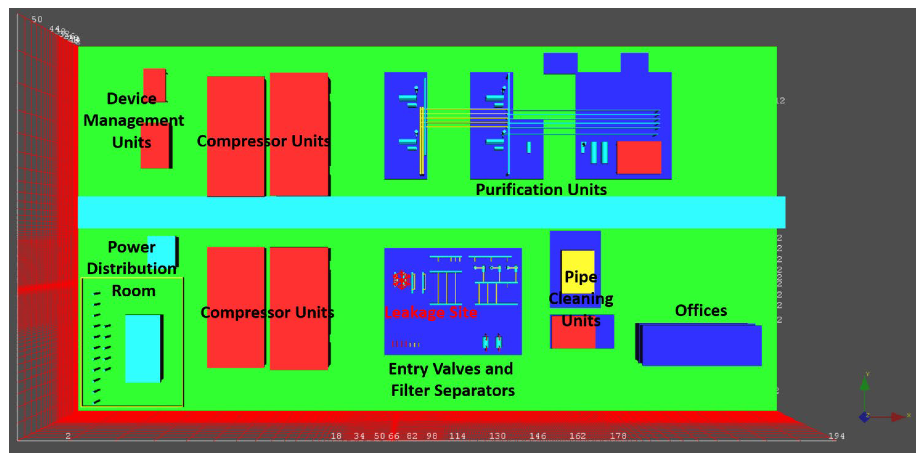
As the initial effort to test the feasibility of using ML algorithms to predict the natural gas dispersion range region, one NGDS was constructed within a 3D computational domain (326 m ×170 m × 40 m) in this in silico investigation based on a local NGDS in Chongqing, China, mimicking the realistic gas dispersion scenarios on site. As shown in Figure 2, it included a series of components, i.e., entry valve units and filter separators, compressor units, purification units, device management units, pipe-cleaning units, and an office.
It is worth mentioning that the underground storage units under the entry valve units and filter separators were not considered in the current investigation, since this study focused on predicting the gas dispersion range due to the leakage in the entry valve units and filter separators with higher leakage probabilities than other units (see Figure 2). A set of three hexahedral meshes (i.e., mesh 01, mesh 02, and mesh 03) with corresponding sizes of 1 m, 2 m, and 3 m was generated using FLACS-CFD 24.1 (Gexcon GexCon AS, Bergen, Norway), which was prepared for the mesh independence test. The final mesh, i.e., mesh 02 with 836,205 computational cells, was decided by balancing the computational time and accuracy, with the relative difference in the dispersion range at the monitoring site (see Figure 2) found to be smaller than 5% by comparing the results from the finest mesh.

2.2.2. Governing Equations

In this study, natural gas consisted of three gases, namely, CH4, C2H6, and C3H8, with corresponding ratios of 91%, 7%, and 2%, respectively. The Reynolds-averaged Navier–Stokes (RANS) model with the k-ε turbulence model was used to predict the gas dispersion range in the developed NGDS. Specifically, the governing equations of mass, momentum, enthalpy, the mass fraction of natural gas Y f , and the mixture fraction of gases ξ can be written in an integral form, that is,
t β V ρ ϕ d V + x i β i ρ u i ϕ d A = x i β i Γ ϕ ϕ x i d A + β V S ϕ + R ϕ d V
where β V is the ratio of the open volume to the total volume of each computational cell; ρ is the density; ϕ is the general variable representing either 1, u i , h , k , ε , Y f , or ξ , respectively; V is the control volume; A is the control volume surface normally pointing outwards in the ith direction; u i is the velocity in the ith direction; β i is a term excluded from the Einstein summation convection in the partial differential equations; Γ ϕ is the effective turbulence diffusion coefficient; S ϕ is the source term for ϕ ; and R ϕ is the additional resistance, turbulence, or heat transfer caused by solid obstructions in the computational domain.

2.2.3. Boundary Conditions

To mimic the realistic gas leakage scenarios, three main parameters, i.e., leakage source, weather, and ground environment, were considered in this study, according to the specific operating conditions and associated risk factors in the NGDS [57]. The leakage source conditions included leakage pressure, leakage pore diameter, and leakage direction. The environmental temperature and wind conditions were related to the weather factors, and the ground environment often considered obstructions such as buildings and equipment. The specific designs for CFD modeling are presented in Table 1, consisting of 500 gas dispersion scenarios. The detailed settings can be accessed in the Supplementary File.
The leakage pressure range was set as 2 to 8 MPa to investigate various initial leakage conditions. The leakage aperture size was set from 5 to 150 mm to capture aperture influences on gas dispersion. The leakage direction included three directions in the coordinate system. The wind speed was set from 0 to 7 m/s, with a wide range from calm to intensive windy conditions. To account for the diversity of actual wind directions, this study included eight primary wind directions, ensuring it could adapt to gas leakage diffusion predictions under various conditions. The ground condition incorporated obstacles to simulate the impact of equipment and buildings on gas diffusion within the NGDS environment.
In this study, atmospheric stability was specifically set as Category F. This selection was grounded in the worst-case-scenario principle in an NGDS leakage and dispersion accident. The high stability and limited vertical mixing characteristic of Category F often led to the maximum accumulation of leaked gas and the largest flammable cloud volumes. By prioritizing these critical conditions, the developed prototype ensures a conservative and reliable safety margin for rapid risk assessment and emergency decision making. The temperature was maintained at 20 °C, providing a standard condition for examining gas dispersion behaviors. The humidity was set at 60% to isolate the humidity variable and assess the effects of other main factors on gas diffusion. The atmospheric pressure was maintained at 0.1 MPa, offering a unified pressure reference to study pressure-related factors in the simulated gas dispersion processing.

2.2.4. Training and Testing Database Preparation

The detailed settings of 500 gas dispersion scenarios can be accessed in the Supplementary File (numbered case001 to case500), which were prepared for the ML training, verification, and testing database. The datasets consisted of five parametric features, i.e., leak pressure, leak aperture size, leak direction, wind speed, and wind direction (see Table 1). The dispersion range contours after the leakage had occurred for 60 s, used for training and testing the ML algorithms, were acquired near the leakage location with a horizontal plane for all CFD simulation cases (see left contour in Figure 1).
To reduce the data dimensionality while still delivering highly reliable and widely accepted hazard representations, the cross-section contour was selected based on two rationales, i.e., gas sensors are often installed at this location, and the dispersion range region is close to the largest cross-sectional area in the horizontal direction. It is worth mentioning that the contour figures were plotted within the natural gas explosion limits from 5% to 15%. An example of the dispersion range contour in the cross-section plane can be found in Figure 1. All contours were stored in BMP format as the training and test database. A total of 500 datasets were used to train and evaluate the investigated ML algorithms. The dataset was randomly split and divided into three folders: training set (70%), verification set (20%), and test set (10%).

2.3. ML Algorithms for Gas Dispersion Range Prediction

2.3.1. BPNN Structure

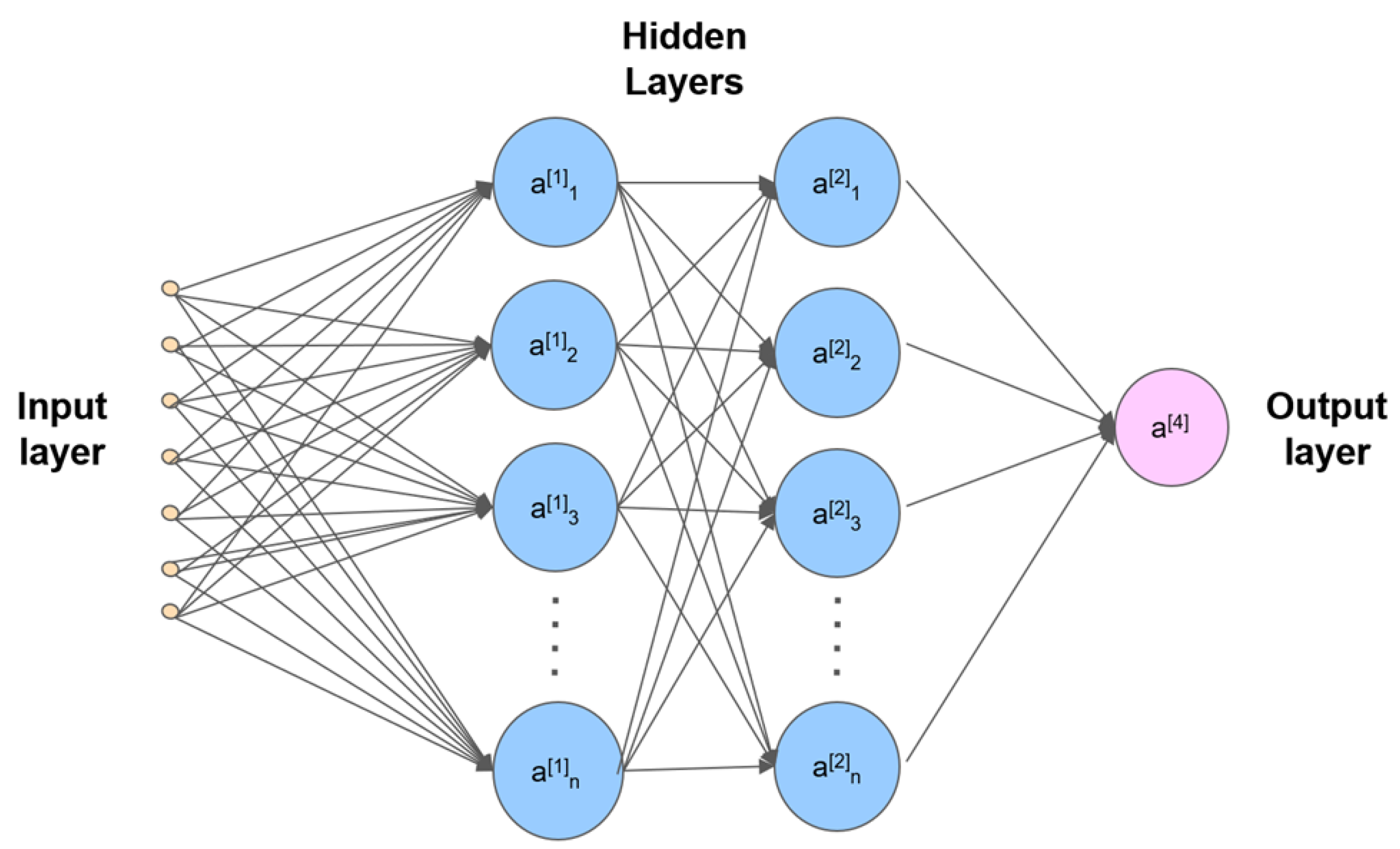
Figure 3 shows the BPNN structure with a multi-layer (a minimum of three layers consisting of input, hidden, and output layers) feedforward network trained by an error inverse propagation algorithm [58]. The learning process of the BPNN consists of forward propagation and backpropagation. In the forward propagation, the features of the training data are fed into the input layer. The calculation formula for the input data can be written as
n i m = j = 1 S m 1 w i m , y j m 1 + b i m , m = 1 , 2 , ,   M   ( M     2 )
where M is the number of layers in the neural network. The predicted output is obtained by passing through the hidden layers. Each neuron weighs the input, and then the output is obtained through the sigmoid activation function. The output of each layer and the last layer of neurons can be obtained using Equations (3) and (4), respectively, which are
y m = f m n m
y = y M
where m is the neural network in each layer, and f m represents the transfer function in each layer.
In backpropagation, the error of the predicted output is calculated by comparing the real value before it is propagated back to the network layer via the chain rule to reduce the error by updating the weight of each neuron. This process involves gradient calculation and then uses gradient descent to adjust the corresponding weight. Using the gradient descent method, the minimum error can be calculated via the partial derivatives of
F ^ ω I , j m = F ^ n i m × n i m ω I , j m
F ^ b i m = F ^ n i m × n i m b i m
where F ^ is the error function; ω I , j m is the connection weight between the i-th neuron and the j-th input in the m-th layer neural network; n i m is the weighted sum of all the input signals received by the i-th neuron in the m-th layer; and b i m is the bias parameter of the i-th neuron in the m-th layer, which provides an adjustable threshold for the neuron and affects the activation state of the neuron.
The weights can be adjusted using
ω I , j m k + 1 = w I , j m ( k ) η s i m y j m 1
b i m k + 1 = b i m ( k ) η s i m
The whole process is repeated until reaching the predetermined number of training rounds or satisfying the terminated conditions. During this process, the BPNN gradually learns the mapping relationship between the input features and the output labels, thereby improving the performance and generalization ability.

2.3.2. LSTM Structure

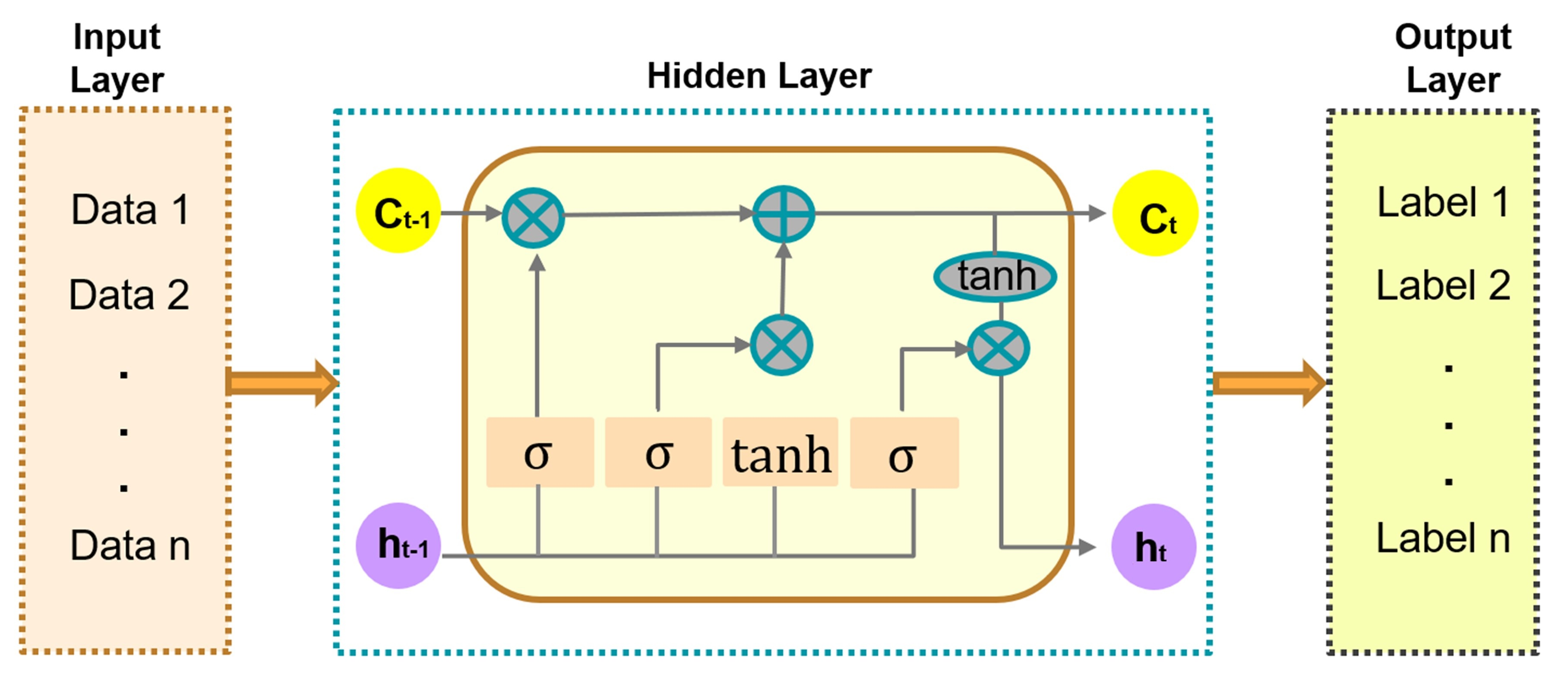
As shown in Figure 4, LSTM has three components, i.e., an input layer, an LSTM layer, and a fully connected output layer, possessing the capability to predict the gas dispersion scenarios with the features in time-series and nonlinear distributions [2,59]. Specifically, the LSTM input layer receives time-series data as inputs, which is the primary source for ML learning and prediction. Each time step contains input data information in various dimensions. The time-series data travel through the input layer into the model, and the features of each time step are passed to the LSTM layer, which processes the input sequence through the input gate, the forget gate, and the output gate, simultaneously adjusting and transmitting hidden states and capturing long-term dependencies in the sequence. In this process, the selected information can be retained by the forget gate using
f t = σ W f h t 1 , x t + b f
where f t represents the output value of the forget gate; W f represents the weight matrix; and σ representative the sigmoid activation function. When f t = 1 , it indicates that the previous moment state is retained. When f t = 0 , it indicates that the previous moment state is discarded.
The unit status is updated by
C t = f t C t 1 + i t C T ~
The outlet results are calculated via the output gate by
o t = σ ( W o h t 1 , x t ) + b o
h t = o t tanh ( C t )
The final results are in the LSTM obtained via a fully connected linear layer, which is responsible for mapping the learned hidden states to target values. The parameters of the fully connected layer are optimized during backpropagation training to minimize the difference between the predicted and real values.

2.3.3. GRU Structure

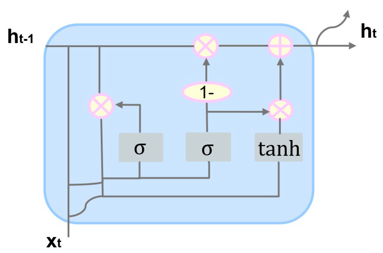
GRU is a varietal LSTM model in recurrent neural networks to improve their performance by replacing the input and forget gates with an update gate. The specific memory and forgetting gates can better solve the problems of gradient vanishing and gradient explosion in the process of time-series training [60]. As presented in Figure 5, the GRU model uses a GRU layer and a linear output layer.
During the forecasting process, the model receives time-series data as the input, where each time step contains multiple features. This input sequence is a key source of information for model learning and prediction. The GRU layer dynamically adjusts and memorizes sequence information through the mechanism of updating and resetting gates. The fully connected layer is responsible for mapping the learned hidden state to target values and generating the final predicted output. Specifically, the mathematical expressions for the update gate and the reset gate in GRU are
n e t z = w z x t + u z h t 1
z t = σ n e t z
where n e t z represents the excitation function; w z and u z are weights; x t represents the input data at the current time; h t 1 represents the hidden state in the previous moment; and z t is the output value of the update gate, and it is obtained by applying the sigmoid activation function σ to n e t z .

2.4. Numerical and ML Setups

In this study, CFD modeling was performed using FLACS-CFD 24.1 (Gexcon GexCon AS, Bergen, Norway) in a local 64-bit Windows workstation with the specifications of an Intel CPU i7-12700 (12 cores; 2.1 GHz) and 64 GB of RAM. The second-order central differencing scheme was employed to obtain diffusive fluxes, and a second-order hybrid scheme with weighting between upwind and central differences was used to obtain convective fluxes. Time marching was carried out using the first-order implicit backward Euler scheme, and the discretized equations were solved using the biconjugate gradient stabilized method (BiCGSTAB), an iterative method, with the semi-implicit method for pressure-linked equations (SIMPLE), a pressure correction algorithm. Each case took ~72 h to match the convergence criteria of 1 × 10⁻⁵.
The four ML algorithms were coded and compiled in Keras 2.4.3. The training and testing were performed on a local 64-bit Windows workstation with an Intel GPU UHD 770 with 32 GB of shared memory. The root-mean-square error (RMSE) was used to measure the difference between the predicted output of a model and the actual target value. The coefficient of determination (R2), mean squared error ( M S E ), mean absolute error ( M A E ), 95% prediction interval coverage (PICP) (95% prediction interval) [61], and false-negative rate (FNR) [62] were used to assess how well a regression model fit the observed data in this study (see Section 3). The training times were approximately 4.23 s, 14.32 s, 20.35 s, and 1.45 s per epoch for the BPNN, LSTM, GRU, and PSO-BPNN models, respectively.

2.5. Data Preprocessing for ML

The dispersion phenomena in NGDSs can be affected by many factors, such as wind speed, direction, obstacles, etc., while the dimensions and magnitude of these features can be quite different [41]. To avoid the influence of the raw data on the prediction range, different features were normalized to make the datasets uniform. Specifically, three steps were taken to preprocess the raw data, i.e.,
Parameters such as leakage pressure, leakage pore diameter, wind speed, temperature, and atmospheric pressure were categorized.
Specific characters of the input data were removed and converted into floating-point number types. For example, wind direction and leakage direction were converted into numeric values using Label Encoder. Specifically, using Label Encoder, the wind directions of east, northeast, north, northwest, west, southwest, south, and southeast were encoded into sequential angular increments of 0°, 45°, 90°, 135°, 180°, 225°, 270°, and 315°, respectively. Using the same pathway, leak directions in X and Y were encoded into 0° (east) and 90° (north), respectively.
Z-score normalization was used to standardize the standard deviation of the data and scale the data according to the mean value of the data. The mean value of the data was 0, and the standard deviation was 1.0.
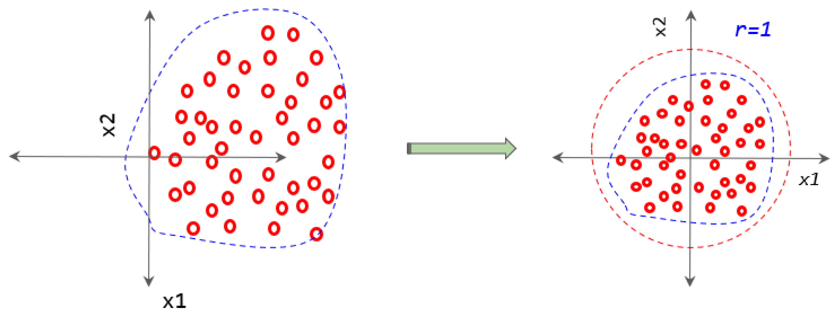
More specifically, Figure 6 illustrates the normalization process, with the raw data on the left and the normalized data on the right, with a mean value of 0 and a variance value of 1.0. This processing can normalize different parameters using the same scale, improving the convergence speed. Z-score normalization can be expressed by
Z = ( x   μ ) σ
where x represents the original sample data values; μ is the mean of the sample data, which is calculated as the average of all the data values in the original dataset; and σ is the standard deviation of the sample data, which measures the dispersion degree.

3. Results and Discussion

3.1. CFD Modeling Validation

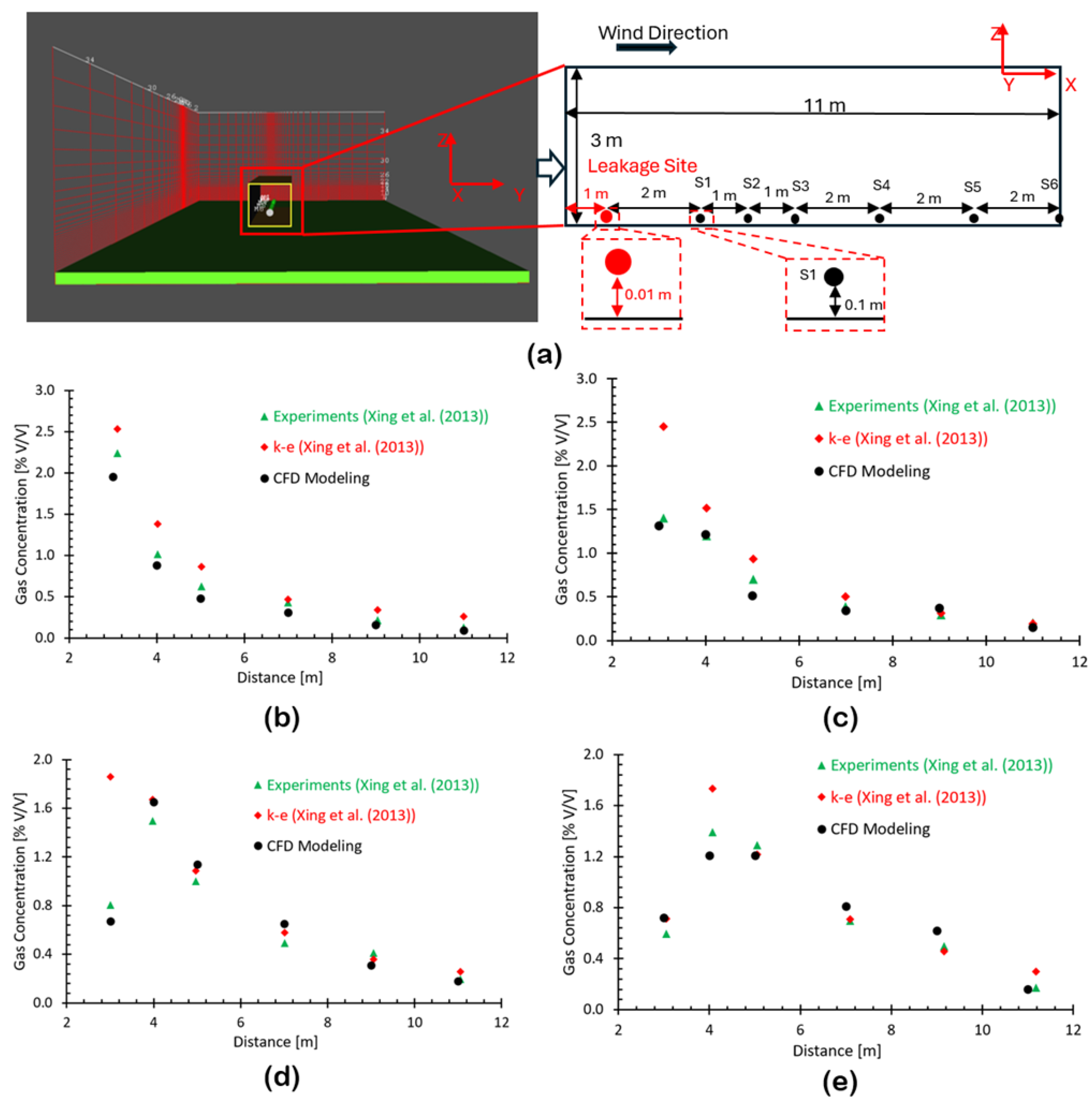
To validate the CFD model, which can be successfully employed to simulate the gas dispersion range in an NGDS, the gas concentrations obtained in this study were compared with previous experimental results and simulation results [63]. As presented in Figure 7a, a full-size wind tunnel (11 × 3 × 3 m3) was constructed, and a mesh independence test was conducted to determine the final mesh with 45,220 hexahedral volumetric cells for CFD modeling by comparing the gas concentration at the sampling point S1 with the results from the finest mesh with 112,466 volumetric cells, in which the computational accuracy and efficiency were considered specifically. The leakage site size was 0.01 m. It was oriented vertically upwards at a height of 0.01 m above the ground and horizontally forwards at 1 m from the air inlet. Four spilling scenarios were simulated with corresponding gas-spilling rates, namely, 10, 12, 15, and 18 m3/h. Since the wind velocity plays a pivotal role in the gas dispersion, according to the experimental settings [63], which considered ground fractional effects, the inlet wind velocity u at different heights Z was designated as
Z = ( x μ ) σ
where u 0 was 0.6 m/s, which was measured at a height of 2 m ( Z 0 ) at the computational center, and p was set as 0.3, since the local atmospheric stability class was F. A total of six sampling points, namely, S1, S2, S3, S4, S5, and S6 (see Figure 7a) were arrayed in the center line via the leakage jet nozzle in the downstream direction. In accordance with the experimental settings, the distances between the leakage site and sampling points (S1–S6) were 2, 3, 4, 6, 8, and 10 m, respectively [63].
It is worth noting that although the baseline experimental validation was conducted using CO2 wind tunnel data [63], the primary objective was to verify the mathematical and numerical robustness of the CFD framework, particularly the efficacy of the selected turbulence model, grid discretization, and species transport equations in resolving complex concentration gradients. Since the fundamental Navier–Stokes and advection–diffusion equations universally govern continuous fluid dispersion, the validated numerical methodology is highly transferable. Transitioning the model to simulate high-pressure natural gas jets fundamentally relies on updating the thermophysical material properties, such as density and molecular weight and the respective boundary conditions within this proven computational architecture, thereby ensuring high confidence in the predictive accuracy of the target natural gas scenarios.
In Figure 7b–e, it can be found that the gas concentrations in the CFD modeling at various distances agreed decently with the experimental data under the simulated four spillage scenarios, with the Pearson correlation coefficients R being larger than 0.9995, 0.9666, 0.9761, and 0.9728, respectively. Such results in this study even performed better than the CFD modeling using the k ε turbulence model in a previous study [63], in which the R values were registered as 0.9946, 0.9752, 0.8121, and 0.9607 under spilling rates of 10, 12, 15, and 18 m3/h, respectively. Therefore, it can be justified that the employed CFD model in this study was qualified to simulate gas dispersion scenarios in the NGDS realistically.

3.2. ML Prediction Performance

The mean squared error ( M S E ), mean absolute error ( M A E ), determination coefficient ( R 2 ), maximum absolute error (MaxAE), 95% prediction interval coverage (PICP) (95% prediction interval) [61], and false-negative rate (FNR) [62] were calculated on the test set to evaluate the prediction accuracy and generalization capability of each ML prediction model in this study. The averaged M S E and M A E , as well as R 2 , are calculated using Equations (17)–(20):
M S E   =   1 N   n   =   1 N y i ~     y i   2
M A E = 1 N   n = 1 N | y i ~ y i   |
R 2 = 1   i = 1 n ( y i ~ y i ) 2 ( y i ¯ y i )
M a x A E = N M a x i = 1 | y i ~ y i   |
where y i represents the actual data value, y i ~ represents the predicted output value from the neural network, y i ¯ represents the mean value of the ground-truth data, and N is the number of tested cases. R 2 ranges from 0 to 1. A value approaching 0 indicates poor model performance, suggesting that the model fails to capture the underlying patterns in the data. Conversely, a value close to 1 signifies excellent predictive ability, reflecting the model’s strong alignment with the observed outcomes and its effectiveness in making accurate predictions. Since the models output deterministic point predictions rather than probabilistic bounds, this study estimated the 95% prediction interval using the standard assumption of normally distributed residuals, i.e., ±1.96 × standard deviation of errors. In FNR evaluation, a false negative means the model failed to predict the gas dispersion range (e.g., the sample critical hazard threshold of 110).

3.2.1. BPNN Performance

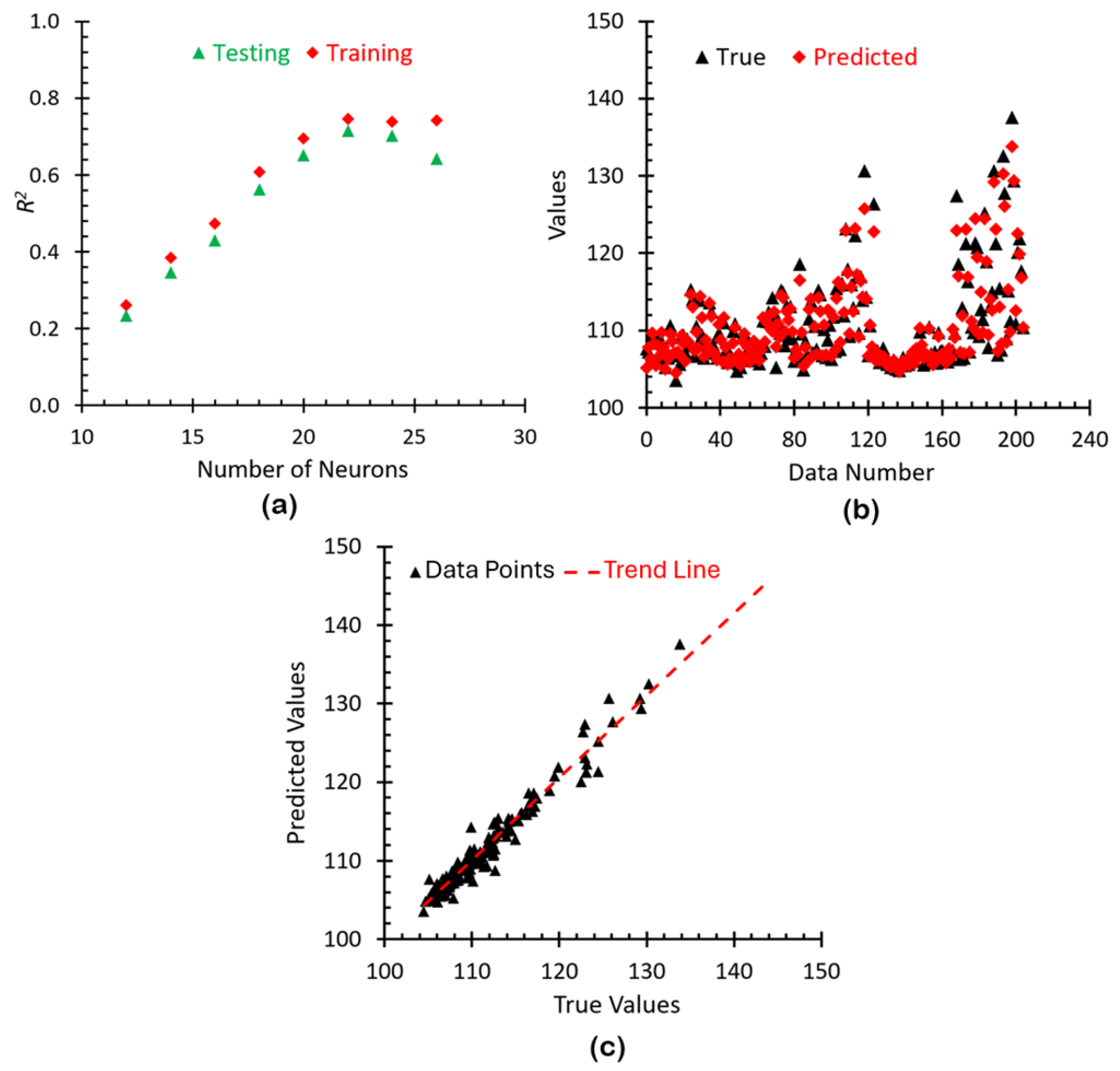
The performance of the BPNN model was estimated by comparing the predicted values with the real simulated values using Scikit-learn MLP Regressor. Specifically, the model sensitivity was investigated first to determine the appropriate number of neurons that were designated to train and test the BPNN algorithms. As shown in Figure 8a, when the neurons in the hidden layer reached 22, the calculated R 2 tended toward a stable state, with a registered value of 0.747 in the training session.
Therefore, 22 neurons were selected as the final algorithmic structure in the hidden layer to predict the gas dispersion range. The sigmoid activation function was used, and the number of iterations was set as 200. The data obtained by comparing the simulated data with the predicted data through the BPNN with hyperparameter tuning are shown in Figure 8b,c, resulting in the BPNN model being able to predict the gas dispersion range in the NGDS well, with R2 = 0.96, MSE = 1.35, MAE = 0.77, MaxAE = 4.94, PICP = 92.68%, and FNR = 6.76% (see Table 2).

3.2.2. LSTM Performance

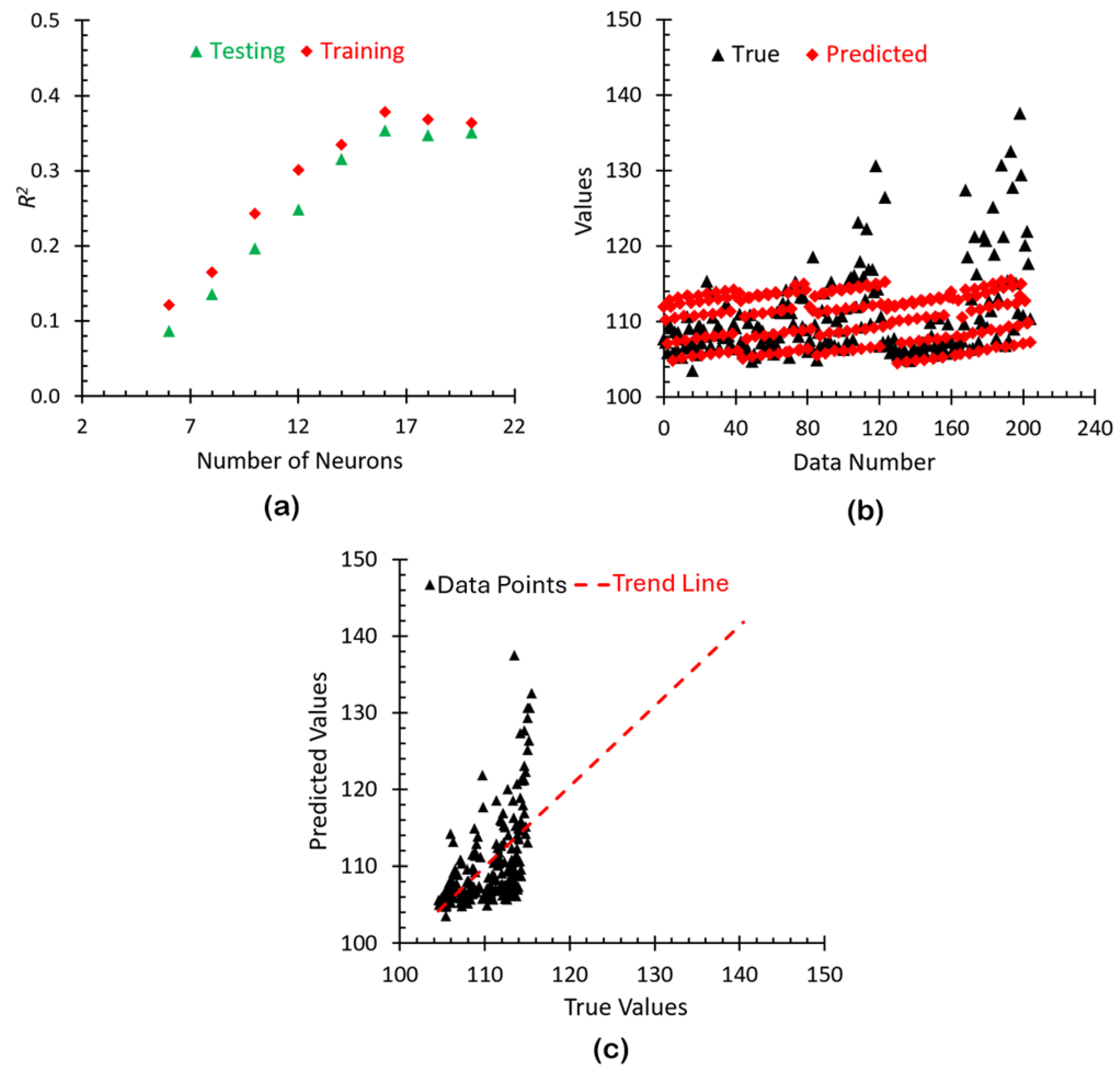
Similar to the investigations of the BPNN model, the sensitivity of LSTM was studied first, and 16 neurons were determined to train and test the LSTM algorithms, whereby a stable R 2 was obtained (see Figure 9a), i.e., 0.37. It is worth mentioning that, in this study, the Adam optimizer was used to update model parameters, and the learning rate was set as 0.001. The MSE was used as the loss function to measure the difference between the model output and the actual label. The number of iterations was set as 200 with the Tanh activation function. The performance of the LSTM model is visualized in Figure 9b,c by hyperparameter tuning (R2 = 0.32, MSE = 23.25, MAE = 3.43, MaxAE = 24.15, PICP = 95.10%, and FNR = 16.44% (see Table 2)) after epochs.

3.2.3. GRU Performance

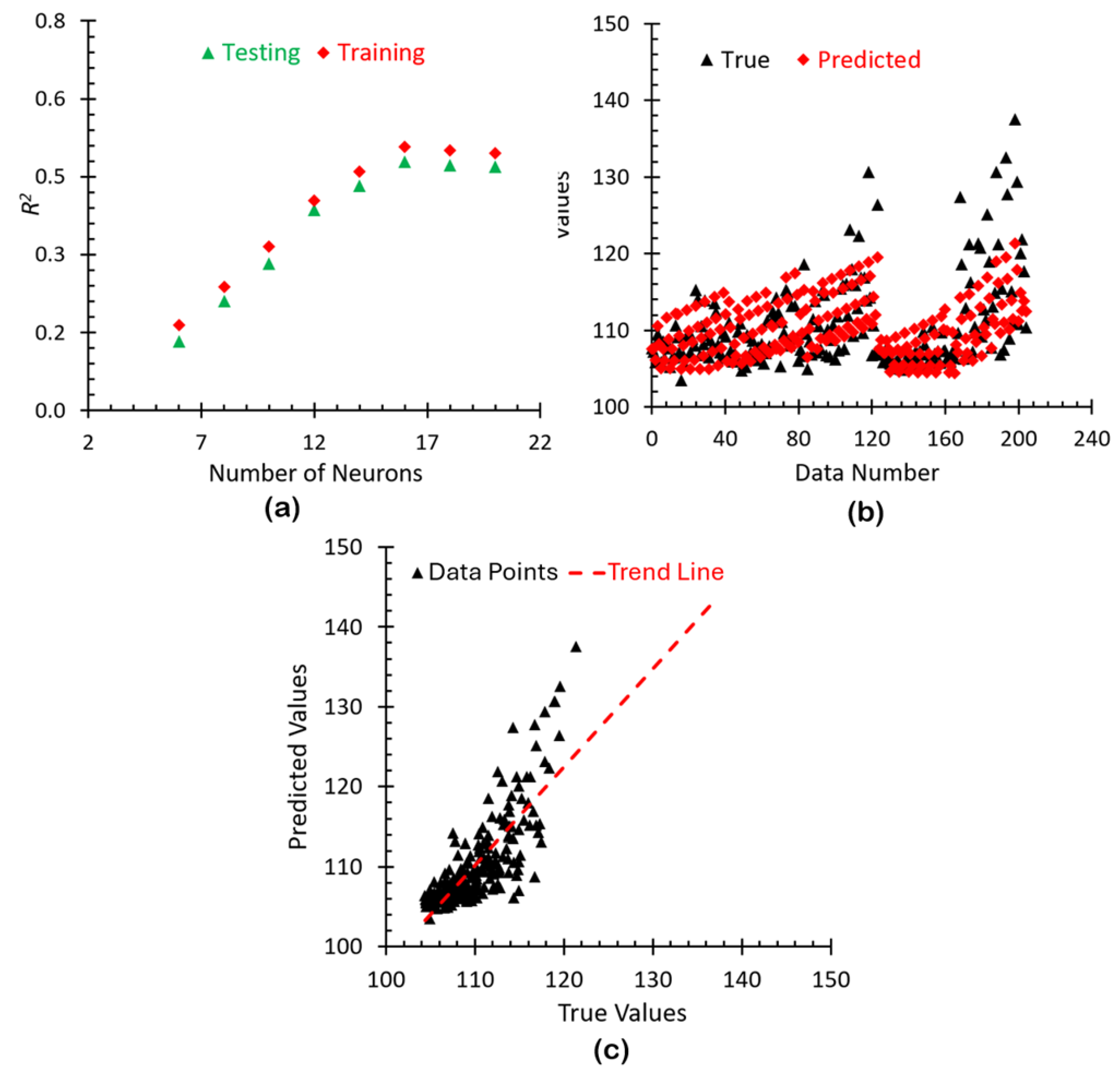
The sensitivity of the GRU model was investigated first by comparing the results with varying numbers of neurons. As shown in Figure 10a, R 2 reached a stable state, with a registered value of 0.542, as the neurons were increased to 16 in the training session. Thus, the final structure of the GRU model consisted of 16 neurons in the hidden layer. In the prediction process, one GRU layer and 11 hidden layers were employed, and the Adam optimizer was used to update the model parameters. The learning rate was set to 0.001 with the Tanh activation function. Figure 10b,c show the evaluations (R2 = 0.63, MSE = 13.41, MAE =2.49, MaxAE = 16.21, PICP = 93.66%, and FNR = 9.46% (see Table 2)) after epochs by comparing the hyperparameter tuning between true and predicted values.

3.3. PSO-BPNN Model Performance

It can be found from Section 3.2 that the capabilities of the GRU model and the LSTM model in predicting the gas dispersion range in the NGDS were lower than the performance of the BPNN model, although all employed algorithms were discreetly adjusted through cross-validation to ensure their optimal performance. Even for BPNN model, the accuracy (R2 = 0.96, MSE = 1.35, MAE = 0.77, MaxAE = 4.94, PICP = 92.68%, and FNR = 6.76%) in the gas dispersion range prediction cannot satisfy the practical conditions, since more accurate information upon the dispersion range in gas leakage accidents is mandatory to ensure the instant emergency response is carried out to reduce the loss from leakage consequences.
Nevertheless, it is worth mentioning that the superior performance of the BPNN over the other two sequence-based models (i.e., LSTM and GRU) can be primarily attributed to data suitability. The input features utilized in this study (i.e., leak pressure, leak aperture size, leak direction, wind speed, and wind direction) represent independent boundary conditions for distinct dispersion scenarios at t = 60 s rather than continuous time-series data. While LSTM and GRU are explicitly designed to capture temporal or sequential dependencies through complex internal gating mechanisms, the current dataset lacks a meaningful sequential structure for these architectures to exploit. Consequently, applying sequence-based models to non-sequential, independent spatial parameters introduces unnecessary algorithmic complexity, leading to their considerable underperformance. In contrast, the BPNN effectively establishes direct, nonlinear mappings between independent input variables and the spatial dispersion outputs, making it fundamentally better suited for the dataset evaluated in this study.
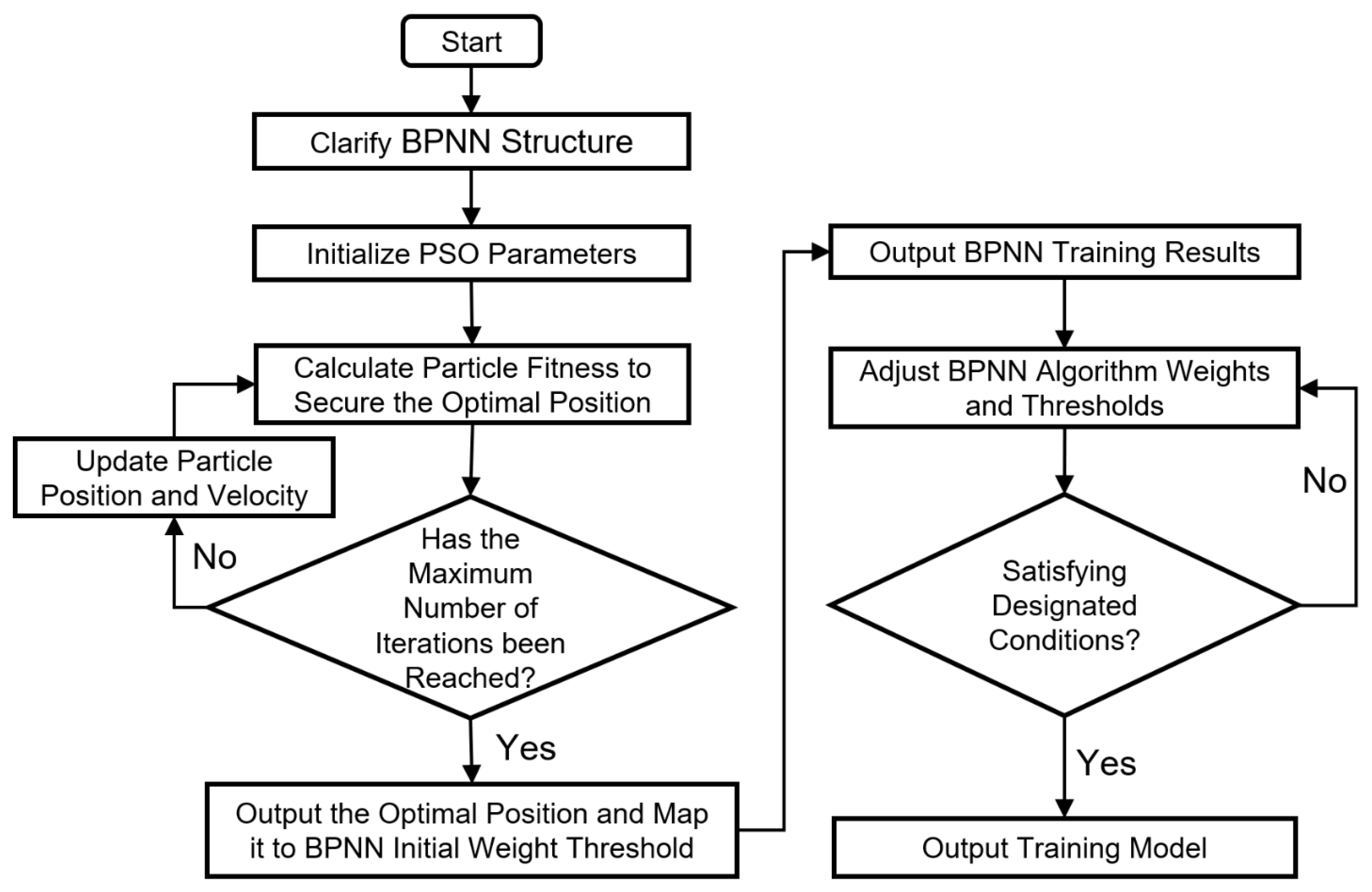
In this study, although the BPNN model has good applicability to dealing with nonlinear problems, it is prone to overfitting [44]. The BPNN model is not only time-consuming but also has intensive needs for cache during the prediction process. Local suboptimal solutions and high calculation costs limit its application as well. Alternatively, a previous study revealed that PSO algorithms assembled in the BPNN model have the capability to reduce learning time and stabilize network training [41]; thus, this study made a tentative effort to test the qualifications of the PSO-BPNN model in predicting gas dispersion range in gas leakage accidents. The program employed the synthesis of the BPNN and PSO algorithms to deliver a top-tier solution for predicting the leakage range of combustible gases in NGDSs by enhancing the optimization of neural network weights and thresholds. The specific processes of establishing the PSO-BPNN model are shown in Figure 11.
Specifically, in the process of finding the optimal value, the BPNN structure was first defined, and the particle swarm parameters were initialized; that is, the number, velocities and positions of particles in the PSO algorithm were determined. Then, the fitness of each particle was calculated to ensure an optimal position. The quality of the solution represented by each particle was assessed to determine its location in the search space. The positions and velocities of the particles were updated based on their fitness and the principles of PSO algorithms. The formulae for calculating particle velocity and position were as follows:
v i d ( t + 1 ) = w × v i d ( t ) + c 1 r 1 p id x id ( t ) + c 2 r 2 ( p gd x id ( t ) )
x id ( t + 1 ) = x id ( t ) + v id ( t + 1 )
where c 1   and c 2   represent the learning factors in the range of (0, 2); v i d represents the velocity of particle motion; x i d represents the position of the particle; and r 1   and   r 2 represent numerical values in the range of (0, 1).
After updating the particles’ positions and velocities, it was checked whether the predetermined maximum number of iterations had been reached. If not, the particles’ positions and velocities were continuously updated until either the maximum number of iterations was reached, or other stopping criteria were satisfied. The optimal particle position was chosen as the initial weight and threshold of the neural network. These initial weights and thresholds were then used to train the neural network using the BPNN algorithms. During the training process, the BPNN algorithms continuously adjusted the weights and thresholds to minimize errors. Finally, it was checked whether the training had satisfied the designated end conditions, such as reaching a predetermined error threshold or completing a predetermined number of iterations. If the end condition was met, the trained neural network model was the final output.
In the computing process, the population size (i.e., the number of particles) was set as 20 based on previous research [39] and the characteristics of the predicted data in this work. The dimension value of a single particle was calculated using
Z = a × h + h × b + h + b
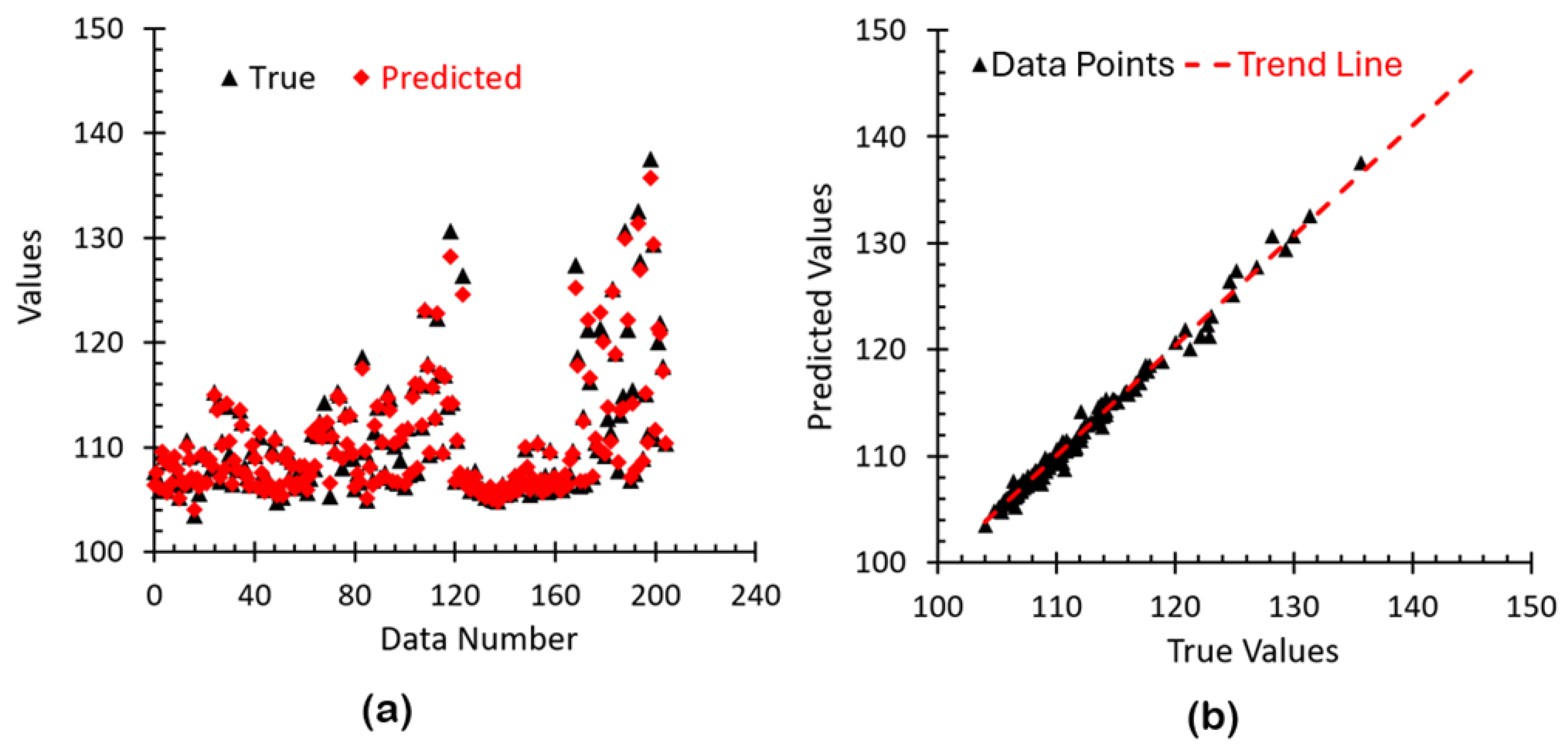
In this study, the particle dimension value was set as 542, and the velocity and position variables of the particles were initialized within (0, 1). The learning factor was set as 2, and the number of iterations was set as 100. In addition, the maximum and minimum inertia weights ω M a x   and   ω M a x were set as 0.8 and 0.4, respectively. By randomly selecting test samples and comparing the output values of the test samples with the simulated values, the reliability of the model was determined and finally reinforced. As shown in Figure 12a,b, the predicted values using the PSO-BPNN model had good performance in matching the CFD values, with R2 = 0.99, MSE = 0.34, MAE = 0.39, MaxAE = 2.47, PICP = 92.68%, and FNR = 0 (see Table 2). More specifically, by comparing the metrics’ values for the four employed models, it can be observed that
PICP 95% comparisons demonstrated that all models hovered around 92~95%, showing normal residual distributions.
The PSO-BPNN achieved a near-perfect R2 = 0.9901 and drastically lowered the MaxAE compared with the other models. It was also unequivocally proven that LSTM and GRU performed poorly on this dataset, with R2 = 0.3184 and 0.6059, respectively.
Using the threshold of 110, the PSO-BPNN never failed to predict a critical value (0% FNR), making it highly reliable for safety predictions. However, it should be mentioned that this threshold needs to be adjusted based on the specific protocol.
Therefore, the PSO algorithms realized the target of sharing information among all particles by learning the local experience for every single particle, which can obtain the global solution in the search space, making up for the shortcomings of the employed BPNN when used solely. Indeed, the standard and unoptimized BPNN serves as the primary internal baseline to demonstrate the exact performance gains achieved by introducing an optimization algorithm. The improved BPNN model (i.e., PSO-BPNN) inherits the adaptive learning ability from the original BPNN model, offering an arbitrary nonlinear map through local search [64]. Integrating the advantages of both the PSO and BPNN models, the employed PSO-BPNN model greatly improved the accuracy and efficiency of ML algorithms to predict gas dispersion ranges in NGDSs.
Although PSO demonstrates significant effectiveness in optimizing the BPNN parameters for this initial prototype, we still plan to incorporate a systematic comparison of various optimization algorithms, such as genetic algorithms (GAs) [65], to identify the most computationally efficient approach for NGDS leakage prediction frameworks. Nevertheless, it is worth mentioning that GAs rely on heavily discrete evolutionary operators, such as crossover and mutation, which are more suitable for discrete domains. PSO utilizes continuous velocity-based updating that is inherently designed for continuous optimization problems [66]. Recent comparative studies evaluating neural network optimizers consistently demonstrated that PSO converges faster than a GA when searching the continuous and high-dimensional weight and bias space of neural architectures [67]. Furthermore, direct benchmark comparisons between the PSO-BPNN and GA-BPNN models in engineering applications [68] confirmed that the PSO-BPNN achieves superior prediction accuracy and computational efficiency.

4. Conclusions

In this study, an experimentally validated CFD model for predicting NGDS leakage dispersion scenarios was developed to secure training and testing datasets under 500 designated leakage scenarios. Then, three ML algorithms, i.e., BPNN, LSTM, and GRU, were employed and compared in terms of their dispersion prediction performance. To further improve prediction accuracy and efficiency, a tentative effort, that is, employing PSO-BPNN algorithms, was made accordingly. The main conclusions are listed below:
An experimentally validated CFD model was developed to predict natural gas leakage dispersion scenarios, and 500 leakage scenarios were simulated accordingly, which were used as the training and testing database.
The prediction results based on the initial three ML models, i.e., BPNN, LSTM, and GRU, showed that the BPNN model had the best performance, with R2 = 0.96, but the shortest time consumption of 4.23 s per epoch.
The proposed PSO-BPNN model achieved a high prediction accuracy (R2 = 0.99), with an average training time of 1.42 s per epoch on the current workstation.
The developed CFD-ML prototype holds great potential for predicting gas dispersion ranges at NGDSs by providing accurate and efficient information to emergency responders, enhancing their ability to swiftly and effectively address leakage incidents.

5. Limitations and Future Study

Although the PSO-BPNN framework demonstrated high prediction accuracy (R2 = 0.99, MSE = 0.34, MAE = 0.39, and MaxAE = 2.47), with an average training time of 1.42 s per epoch, this preliminary study relied on a single NGDS geometry under controlled, fixed weather conditions (e.g., constant atmospheric stability and humidity). Real-world applicability is constrained by the absence of multi-leak interactions, transient weather dynamics, and complex terrain variations. To address these unresolved gaps and realize the full potential of this digital twin framework for emergency responders, future research is planned to focus on the following cutting-edge aspects:
(1)
Integration of transient and realistic meteorological dynamics: Future CFD simulations will incorporate time-varying weather conditions, including transient wind gusts, temperature inversions, varying atmospheric stability classes, and humidity fluctuations. Expanding the dataset to include these dynamic environmental factors will improve CFD modeling robustness in highly unpredictable real-world climates.
(2)
Geometric generalization via cross-domain transfer learning: To move beyond a single NGDS layout, our future work will generate simulation data across various realistic station topologies and complex terrains. By employing cross-domain transfer learning, the model can be generalized to predict dispersion ranges across different hazardous facilities without requiring extensive retraining from scratch for each new site.
(3)
Complex leakage scenarios and multi-source interactions: Real-world accidents often involve compounding failures; therefore, our subsequent studies will expand the predictive framework to account for complex scenarios, such as simultaneous multi-point leaks, transient release rates (e.g., decaying pressure over time), and the mitigating effects of secondary physical containments or blast walls.
(4)
Real-time adaptive learning with live sensor networks: To fully transition the model into a live digital twin, we plan to explore dynamically updating the ML framework using continuous, live data feeds from on-site IoT gas detectors and anemometers. This adaptive learning approach would allow the dispersion contours to be self-corrected in real-time as an emergency unfolds.
(5)
Although the consistent superiority of the PSO-BPNN framework across all these varied statistical dimensions effectively validates its generalization ability on unseen scenarios, as the framework is scaled to encompass broader datasets and dynamic transient leakages in future studies, standard cross-validation protocols will be integrated to further solidify reliability assessments.
(6)
Explainable AI (XAI) for safety-critical decision support: Because machine learning models often operate as black boxes, future iterations will integrate explainable AI techniques (such as SHAP or LIME). This will ensure the interpretability of the model’s predictions, allowing emergency responders and safety engineers to understand the specific weight of input parameters driving a predicted hazard zone, thereby increasing trust in safety-critical applications.

Supplementary Materials

The following supporting information can be downloaded at https://www.mdpi.com/article/10.3390/fluids11060137/s1. Table S1: Supplementary File.

Author Contributions

Conceptualization, H.M.; methodology, H.M. and R.Z.; software, R.Z. and H.Y.; validation, Y.F. and H.Y.; formal analysis, R.Z. and H.Y.; investigation, S.C., R.Z., N.L., A.H., P.S., S.W., Y.N., W.W., G.T. and H.Y.; resources, H.M. and Y.F.; data curation, R.Z., S.C. and H.Y.; writing—original draft preparation, R.Z. and H.Y.; writing—review and editing, H.M., S.C., N.L., A.H., Y.F., P.S., S.W., Y.N., W.W., G.T. and H.Y.; visualization, R.Z. and H.Y.; supervision, H.M. and Y.F.; project administration, H.M.; funding acquisition, H.M. All authors have read and agreed to the published version of this manuscript.

Funding

This work was financially supported by the National Natural Science Foundation of China (NSFC 5227-4177; 5170-4054), the Natural Science Foundation of Chongqing Scientific and Technological (CSTB2023NSCQ-MSX0862), and the Chongqing Construction Science and Technology Program (Task Letter No. Chengkezi 2024 No. 6-7).

Institutional Review Board Statement

Not applicable.

Informed Consent Statement

Not applicable.

Data Availability Statement

The datasets generated and/or analyzed during the current study are available from the corresponding author upon reasonable request.

Conflicts of Interest

Author Geng Tang was employed by the company Southwest Oil and Gas Field Branch, China National Petroleum Corporation (China), Beijing, China. The remaining authors declare that this research was conducted in the absence of any commercial or financial relationships that could be construed as a potential conflict of interest.

Abbreviations

The following abbreviations are used in this manuscript:
AIArtificial intelligence
ANNArtificial neural network
BPNNBackpropagation neural network
BiCGSTABBiconjugate gradient stabilized method
CEEMDANComplete ensemble empirical mode decomposition with adaptive noise algorithm
CFDComputational fluid dynamics
FNRFalse-negative rate
GRUGated recurrent unit network
LSTMLong short-term memory
MAEMean absolute error
MaxAEMaximum absolute error
MSEMean square error
NGDSNatural gas distribution station
PICPPrediction interval coverage
PSOParticle swarm optimization
RANSReynolds averaged Navier–Stokes
RMSERoot-mean-square error
RNNRecurrent neural network

References

  1. Li, X.; Zhao, H.; Zhang, R.; Wang, J. Risk area classification for flammable gas dispersion in natural gas distribution station. J. Loss Prev. Process Ind. 2023, 86, 105202. [Google Scholar] [CrossRef] [Scilit]
  2. Song, D.; Lee, K.; Phark, C.; Jung, S. Spatiotemporal and layout-adaptive prediction of leak gas dispersion by encoding-prediction neural network. Process Saf. Environ. Prot. 2021, 151, 365–372. [Google Scholar] [CrossRef] [Scilit]
  3. Wang, D.; Liang, P.; Yu, Y.; Fu, X.; Hu, L. An integrated methodology for assessing accident probability of natural gas distribution station with data uncertainty. J. Loss Prev. Process Ind. 2019, 62, 103941. [Google Scholar] [CrossRef] [Scilit]
  4. Yi, H.; Feng, Y.; Wang, Q. Computational fluid dynamics (CFD) study of heat radiation from large liquefied petroleum gas (LPG) pool fires. J. Loss Prev. Process Ind. 2019, 61, 262–274. [Google Scholar] [CrossRef] [Scilit]
  5. Yi, H.; Feng, Y.; Park, H.; Wang, Q. Configuration predictions of large liquefied petroleum gas (LPG) pool fires using CFD method. J. Loss Prev. Process Ind. 2020, 65, 104099. [Google Scholar] [CrossRef] [Scilit]
  6. Weller, Z.D.; Hamburg, S.P.; von Fischer, J.C. A National Estimate of Methane Leakage from Pipeline Mains in Natural Gas Local Distribution Systems. Environ. Sci. Technol. 2020, 54, 8958–8967. [Google Scholar] [CrossRef] [Scilit]
  7. Koopman, R.P.; Cederwall, R.T.; Ermak, D.L.; Goldwire, H.C.; Hogan, W.J.; McClure, J.W.; McRae, T.G.; Morgan, D.L.; Rodean, H.C.; Shinn, J.H. Analysis of burro series 40-m3 lng spill experiments. Hazard. Mater. 1982, 6, 43–83. [Google Scholar] [CrossRef] [Scilit]
  8. Montiel, H.; Vílchez, J.A.; Casal, J.; Arnaldos, J. Mathematical modelling of accidental gas releases. Hazard. Mater. 1998, 59, 211–233. [Google Scholar] [CrossRef] [Scilit]
  9. Fang, H.; Xue, H.; Bao, C.; Tang, W. Characteristics of gas leakage and typical dispersion modes for FPSO’s process modules. Ocean Eng. 2022, 266, 113117. [Google Scholar] [CrossRef] [Scilit]
  10. Puttock, J.S.; Blackmore, D.R.; Colenbrander, G.W. Field experiments on dense gas dispersion. J. Hazard. Mater. 1982, 6, 13–41. [Google Scholar] [CrossRef] [Scilit]
  11. Dong, S.-E.; He, Y.; Dong, J.; Peng, Z.; Fu, G. A Review of Leakage and Dispersion of LNG on the Ground. Energy Eng. 2021, 118, 103–118. [Google Scholar] [CrossRef] [Scilit]
  12. Briggs, G.A.; Britter, R.E.; Hanna, S.R.; Havens, J.A.; Robins, A.G.; Snyder, W.H. Dense gas vertical diffusion over rough surfaces: Results of wind-tunnel studies. Atmos. Environ. 2001, 35, 2265–2284. [Google Scholar] [CrossRef] [Scilit]
  13. Shen, R.; Jiao, Z.; Parker, T.; Sun, Y.; Wang, Q. Recent application of Computational Fluid Dynamics (CFD) in process safety and loss prevention: A review. J. Loss Prev. Process Ind. 2020, 67, 104252. [Google Scholar] [CrossRef] [Scilit]
  14. Verfondern, K.; Dienhart, B. Pool spreading and vaporization of liquid hydrogen. Int. J. Hydrogen Energy 2007, 32, 2106–2117. [Google Scholar] [CrossRef] [Scilit]
  15. Luketa-Hanlin, A. A review of large-scale LNG spills: Experiments and modeling. J. Hazard. Mater. 2006, 132, 119–140. [Google Scholar] [CrossRef] [Scilit]
  16. Krogstad, P.A.; Pettersen, R.M. Windtunnel modelling of a release of a heavy gas near a building. Atmos. Environ. (1967) 1986, 20, 867–878. [Google Scholar] [CrossRef] [Scilit]
  17. Chan, S.T. Numerical simulations of LNG vapor dispersion from a fenced storage area. J. Hazard. Mater. 1992, 30, 195–224. [Google Scholar] [CrossRef] [Scilit]
  18. Roberts, P.T.; Hall, D.J. Wind-tunnel simulation. Boundary layer effects in dense gas dispersion experiments. J. Loss Prev. Process Ind. 1994, 7, 106–117. [Google Scholar] [CrossRef] [Scilit]
  19. Tauseef, S.M.; Rashtchian, D.; Abbasi, S.A. CFD-based simulation of dense gas dispersion in presence of obstacles. J. Loss Prev. Process Ind. 2011, 24, 371–376. [Google Scholar] [CrossRef] [Scilit]
  20. Zhang, K.; Tan, C.; Lv, Z.; Chen, R. Study on LNG leakage and diffusion in dangerous goods logistics park. IOP Conf. Ser. Earth Environ. Sci. 2021, 657, 012033. [Google Scholar] [CrossRef] [Scilit]
  21. Britter, R.E. Modelling Dispersion from Accidental Releases. In Air Pollution Modeling and Its Application VII; van Dop, H., Ed.; Springer: Boston, MA, USA, 1989; pp. 39–52. [Google Scholar]
  22. Witlox, H.W.M. The HEGADAS model for ground-level heavy-gas dispersion—I. Steady-state model. Atmos. Environ. 1994, 28, 2917–2932. [Google Scholar] [CrossRef] [Scilit]
  23. Spicer, T.; Havens, J.; Guinnup, D. User’s Guide for the DEGADIS 2.1 Dense Gas Dispersion Model; US Environmental Protection Agency: Washington, DC, USA, 1989.
  24. Ermak, D.L. User’s Manual for SLAB: An Atmospheric Dispersion Model for Denser-than-Air-Releases; Lawrence Livermore National Laboratory: Livermore, CA, USA, 1990.
  25. Vílchez, J.A.; Villafañe, D.; Casal, J. A dispersion safety factor for LNG vapor clouds. J. Hazard. Mater. 2013, 246–247, 181–188. [Google Scholar] [CrossRef] [Scilit]
  26. Fiates, J.; Santos, R.R.C.; Neto, F.F.; Francesconi, A.Z.; Simoes, V.; Vianna, S.S.V. An alternative CFD tool for gas dispersion modelling of heavy gas. J. Loss Prev. Process Ind. 2016, 44, 583–593. [Google Scholar] [CrossRef] [Scilit]
  27. Mishra, K.B. CFD model for large hazardous dense cloud spread predictions, with particular reference to Bhopal disaster. Atmos. Environ. 2015, 117, 74–91. [Google Scholar] [CrossRef] [Scilit]
  28. Tan, W.; Liu, X.; Liu, Y.; Bu, Y.; Wang, Z. Modeling the two-phase cloud evolution from instantaneous flashing release using CFD. J. Loss Prev. Process Ind. 2011, 24, 420–425. [Google Scholar] [CrossRef] [Scilit]
  29. Jiao, Z.; Ji, C.; Sun, Y.; Hong, Y.; Wang, Q. Deep learning based quantitative property-consequence relationship (QPCR) models for toxic dispersion prediction. Process Saf. Environ. Prot. 2021, 152, 352–360. [Google Scholar] [CrossRef] [Scilit]
  30. Hutton, D.; Ponton, J.W.; Waters, A. AI applications in process design, operation and safety. Knowl. Eng. Rev. 1990, 5, 69–95. [Google Scholar] [CrossRef] [Scilit]
  31. Zeng, Y.; Zhang, X.; Su, L.-C.; Wu, X.; Huang, X. Artificial Intelligence tool for fire safety design (IFETool): Demonstration in large open spaces. Case Stud. Therm. Eng. 2022, 40, 102483. [Google Scholar] [CrossRef] [Scilit]
  32. Arunthavanathan, R.; Sajid, Z.; Amin, M.T.; Tian, Y.; Khan, F.; Pistikopoulos, E. Process safety 4.0: Artificial intelligence or intelligence augmentation for safer process operation? AIChE J. 2024, 70, e18475. [Google Scholar] [CrossRef] [Scilit]
  33. Bakas, I.; Kontoleon, K.J. A review of the contributions of Artificial Intelligence in fire engineering, in a world rapidly realising the need for sustainable design. IOP Conf. Ser. Earth Environ. Sci. 2023, 1196, 012112. [Google Scholar] [CrossRef] [Scilit]
  34. Nguyen, H.T.; Nguyen, K.T.Q.; Le, T.C.; Zhang, G. Review on the Use of Artificial Intelligence to Predict Fire Performance of Construction Materials and Their Flame Retardancy. Molecules 2021, 26, 1022. [Google Scholar] [CrossRef] [Scilit]
  35. Ma, D.; Zhang, Z. Contaminant dispersion prediction and source estimation with integrated Gaussian-machine learning network model for point source emission in atmosphere. J. Hazard. Mater. 2016, 311, 237–245. [Google Scholar] [CrossRef] [Scilit]
  36. Han, X.; Zhu, J.; Li, H.; Xu, W.; Feng, J.; Hao, L.; Wei, H. Deep learning-based dispersion prediction model for hazardous chemical leaks using transfer learning. Process Saf. Environ. Prot. 2024, 188, 363–373. [Google Scholar] [CrossRef] [Scilit]
  37. Jiang, Z.; Zhang, Z.; He, X.; Li, Y.; Yuan, H. Efficient and accurate TEC modeling and prediction approach with random forest and Bi-LSTM for large-scale region. Adv. Space Res. 2024, 73, 650–662. [Google Scholar] [CrossRef] [Scilit]
  38. Arunthavanathan, R.; Khan, F.; Ahmed, S.; Imtiaz, S.; Rusli, R. Fault detection and diagnosis in process system using artificial intelligence-based cognitive technique. Comput. Chem. Eng. 2020, 134, 106697. [Google Scholar] [CrossRef] [Scilit]
  39. Alauddin, M.; Khan, F.; Imtiaz, S.; Ahmed, S.; Amyotte, P. Integrating process dynamics in data-driven models of chemical processing systems. Process Saf. Environ. Prot. 2023, 174, 158–168. [Google Scholar] [CrossRef] [Scilit]
  40. Jiao, Z.; Hu, P.; Xu, H.; Wang, Q. Machine Learning and Deep Learning in Chemical Health and Safety: A Systematic Review of Techniques and Applications. ACS Chem. Health Saf. 2020, 27, 316–334. [Google Scholar] [CrossRef] [Scilit]
  41. Al-Andoli, M.N.; Tan, S.C.; Sim, K.S.; Lim, C.P.; Goh, P.Y. Parallel Deep Learning with a hybrid BP-PSO framework for feature extraction and malware classification. Appl. Soft Comput. 2022, 131, 109756. [Google Scholar] [CrossRef] [Scilit]
  42. Kim, H.; Park, M.; Kim, C.W.; Shin, D. Source localization for hazardous material release in an outdoor chemical plant via a combination of LSTM-RNN and CFD simulation. Comput. Chem. Eng. 2019, 125, 476–489. [Google Scholar] [CrossRef] [Scilit]
  43. Shi, J.; Khan, F.; Zhu, Y.; Li, J.; Chen, G. Robust data-driven model to study dispersion of vapor cloud in offshore facility. Ocean Eng. 2018, 161, 98–110. [Google Scholar] [CrossRef] [Scilit]
  44. Na, J.; Jeon, K.; Lee, W.B. Toxic gas release modeling for real-time analysis using variational autoencoder with convolutional neural networks. Chem. Eng. Sci. 2018, 181, 68–78. [Google Scholar] [CrossRef] [Scilit]
  45. Mishra, D.P.; Panigrahi, D.C.; Kumar, P.; Kumar, A.; Sinha, P.K. Assessment of relative impacts of various geo-mining factors on methane dispersion for safety in gassy underground coal mines: An artificial neural networks approach. Neural Comput. Appl. 2020, 33, 181–190. [Google Scholar] [CrossRef] [Scilit]
  46. Bi, Y.; Wu, Q.; Wang, S.; Shi, J.; Cong, H.; Ye, L.; Gao, W.; Bi, M. Hydrogen leakage location prediction at hydrogen refueling stations based on deep learning. Energy 2023, 284, 129361. [Google Scholar] [CrossRef] [Scilit]
  47. Selvaggio, A.Z.; Sousa, F.M.M.; Silva, F.V.d.; Vianna, S.S.V. Application of long short-term memory recurrent neural networks for localisation of leak source using 3D computational fluid dynamics. Process Saf. Environ. Prot. 2022, 159, 757–767. [Google Scholar] [CrossRef] [Scilit]
  48. Sousa, F.M.M.; Selvaggio, A.Z.; Silva, F.V.; Vianna, S.S.V. Leakage source localisation employing 3D-CFD simulations and gated recurrent units. Process Saf. Environ. Prot. 2023, 178, 540–546. [Google Scholar] [CrossRef] [Scilit]
  49. Kopbayev, A.; Khan, F.; Yang, M.; Halim, S.Z. Gas leakage detection using spatial and temporal neural network model. Process Saf. Environ. Prot. 2022, 160, 968–975. [Google Scholar] [CrossRef] [Scilit]
  50. Zhang, X.; Shi, J.; Yang, M.; Huang, X.; Usmani, A.S.; Chen, G.; Fu, J.; Huang, J.; Li, J. Real-time pipeline leak detection and localization using an attention-based LSTM approach. Process Saf. Environ. Prot. 2023, 174, 460–472. [Google Scholar] [CrossRef] [Scilit]
  51. Zhang, X.; Shi, J.; Huang, X.; Xiao, F.; Yang, M.; Huang, J.; Yin, X.; Sohail Usmani, A.; Chen, G. Towards deep probabilistic graph neural network for natural gas leak detection and localization without labeled anomaly data. Expert Syst. Appl. 2023, 231, 120542. [Google Scholar] [CrossRef] [Scilit]
  52. He, X.; Kong, D.; Yu, X.; Ping, P.; Wang, G.; Peng, R.; Zhang, Y.; Dai, X. Prediction model for the evolution of hydrogen concentration under leakage in hydrogen refueling station using deep neural networks. Int. J. Hydrogen Energy 2024, 51, 702–712. [Google Scholar] [CrossRef] [Scilit]
  53. Shi, J.; Xie, W.; Huang, X.; Xiao, F.; Usmani, A.S.; Khan, F.; Yin, X.; Chen, G. Real-time natural gas release forecasting by using physics-guided deep learning probability model. J. Clean. Prod. 2022, 368, 133201. [Google Scholar] [CrossRef] [Scilit]
  54. Wang, R.; Chen, B.; Qiu, S.; Zhu, Z.; Wang, Y.; Wang, Y.; Qiu, X. Comparison of Machine Learning Models for Hazardous Gas Dispersion Prediction in Field Cases. Int. J. Environ. Res. Public Health 2018, 15, 1450. [Google Scholar] [CrossRef] [Scilit]
  55. Tsoukas, V.; Gkogkidis, A.; Boumpa, E.; Papafotikas, S.; Kakarountas, A. A Gas Leakage Detection Device Based on the Technology of TinyML. Technologies 2023, 11, 45. [Google Scholar] [CrossRef] [Scilit]
  56. Kia, S.; Nambiar, M.K.; Thé, J.; Gharabaghi, B.; Aliabadi, A.A. Machine Learning to Predict Area Fugitive Emission Fluxes of GHGs from Open-Pit Mines. Atmosphere 2022, 13, 210. [Google Scholar] [CrossRef] [Scilit]
  57. American Petroleum Institute. Risk-Based Inspection Technology: API Recommended Practice 581; American Petroleum Institute: Washington, DC, USA, 2008. [Google Scholar]
  58. Rumelhart, D.E.; Hinton, G.E.; Williams, R.J. Learning representations by back-propagating errors. Nature 1986, 323, 533–536. [Google Scholar] [CrossRef] [Scilit]
  59. Yao, L.; Zhang, Y.; He, T.; Luo, H. Natural gas pipeline leak detection based on acoustic signal analysis and feature reconstruction. Appl. Energy 2023, 352, 121975. [Google Scholar] [CrossRef] [Scilit]
  60. Cho, K.; van Merriënboer, B.; Gülçehre, Ç.; Bahdanau, D.; Bougares, F.; Schwenk, H.; Bengio, Y. Learning Phrase Representations using RNN Encoder–Decoder for Statistical Machine Translation. In Proceedings of the Conference on Empirical Methods in Natural Language Processing, Doha, Qatar, 25–29 October 2014. [Google Scholar]
  61. Shrestha, D.L.; Solomatine, D.P. Machine learning approaches for estimation of prediction interval for the model output. Neural Netw. 2006, 19, 225–235. [Google Scholar] [CrossRef] [Scilit] [PubMed]
  62. Tighe, P.J.; Harle, C.A.; Hurley, R.W.; Aytug, H.; Boezaart, A.P.; Fillingim, R.B. Teaching a Machine to Feel Postoperative Pain: Combining High-Dimensional Clinical Data with Machine Learning Algorithms to Forecast Acute Postoperative Pain. Pain Med. 2015, 16, 1386–1401. [Google Scholar] [CrossRef] [Scilit]
  63. Xing, J.; Liu, Z.; Huang, P.; Feng, C.; Zhou, Y.; Zhang, D.; Wang, F. Experimental and numerical study of the dispersion of carbon dioxide plume. J. Hazard. Mater. 2013, 256–257, 40–48. [Google Scholar] [CrossRef] [Scilit]
  64. Bhattacharya, U.; Parui, S.K. Self-adaptive Learning Rates in Backpropagation Algorithm Improve Its Function Approximation Performance. In Proceedings of the ICNN’95—International Conference on Neural Networks, Perth, Australia, 27 November–1 December 1995; pp. 2784–2788. [Google Scholar]
  65. Goldberg, D.E.; Holland, J.H. Genetic Algorithms and Machine Learning. Mach. Learn. 1988, 3, 95–99. [Google Scholar] [CrossRef] [Scilit]
  66. Kachitvichyanukul, V. Comparison of three evolutionary algorithms: GA, PSO, and DE. Ind. Eng. Manag. Syst. 2012, 12, 215–223. [Google Scholar] [CrossRef] [Scilit]
  67. Munsarif, M.; Sam’an, M.; Fahrezi, A. Convolution neural network hyperparameter optimization using modified particle swarm optimization. Bull. Electr. Eng. Inform. 2024, 13, 1268–1275. [Google Scholar] [CrossRef] [Scilit]
  68. Cai, B.; Lin, X.; Fu, F.; Wang, L. Postfire residual capacity of steel fiber reinforced volcanic scoria concrete using PSO-BPNN machine learning. Structures 2022, 44, 236–247. [Google Scholar] [CrossRef] [Scilit]
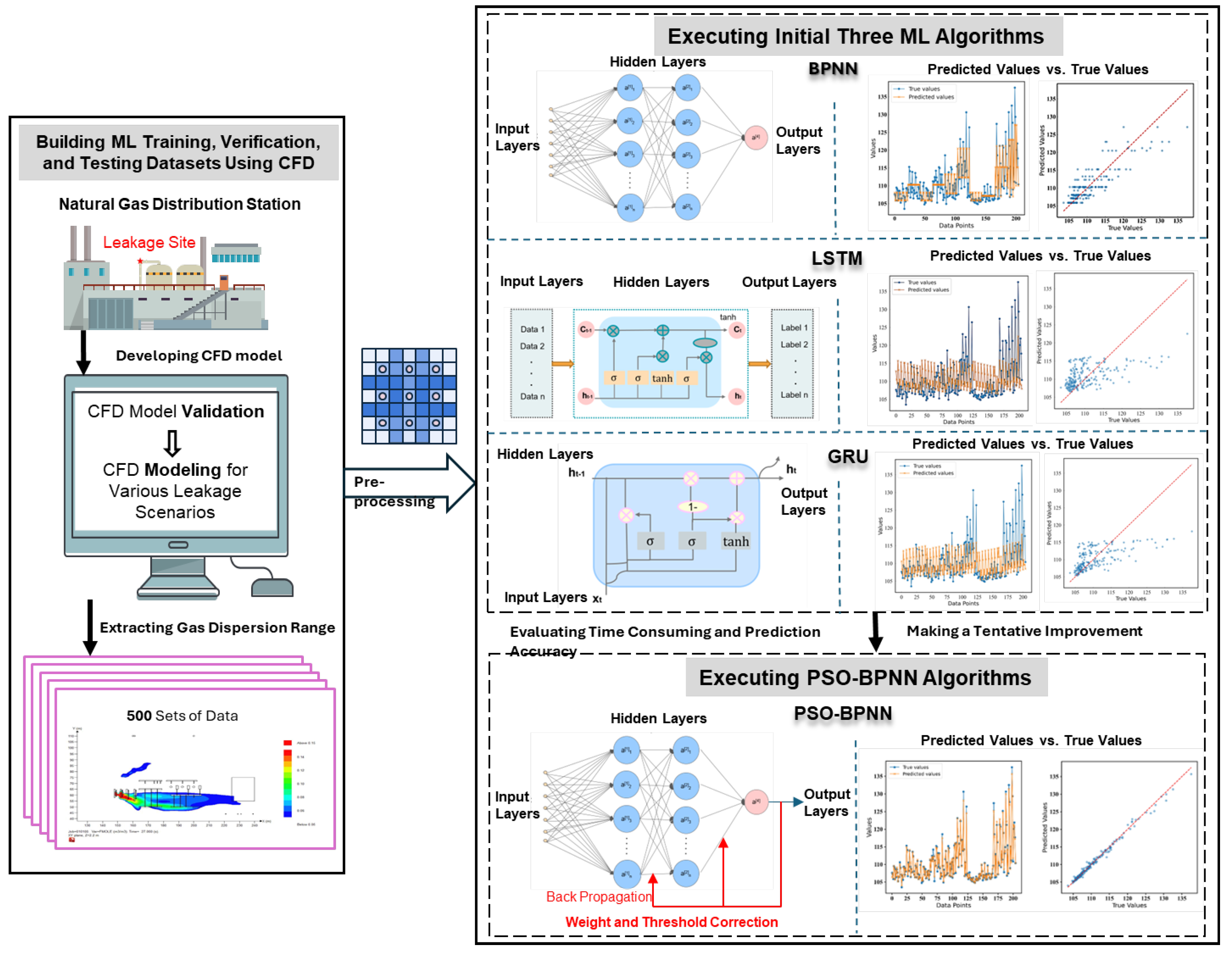
Figure 1. The CFD-ML framework to predict gas dispersion range in a virtual NGDS.
Fluids 11 00137 g001
Figure 2. Layouts and meshes of the NGDS model.
Fluids 11 00137 g002
Figure 3. BPNN structure.
Fluids 11 00137 g003
Figure 4. LSTM network structure.
Fluids 11 00137 g004
Figure 5. GRU network structure.
Fluids 11 00137 g005
Figure 6. Z-score normalization for CFD modeling data.
Fluids 11 00137 g006
Figure 7. CFD model validation [63]. (a) Geometric layouts and sampling sites; (b) comparisons at a release rate of 10 m3/s; (c) comparisons at a release rate of 12 m3/s; (d) comparisons at a release rate of 15 m3/s; and (e) comparisons at a release rate of 18 m3/s.
Fluids 11 00137 g007
Figure 8. BPNN prediction performance. (a) Relationship between neuron number and R2; (b) comparisons between true and predicted data; and (c) scatter distributions for true vs. predicted data.
Fluids 11 00137 g008
Figure 9. LSTM prediction performance. (a) Relationship between neuron number and R2; (b) comparisons between true and predicted data; and (c) scatter distributions for true vs. predicted data.
Fluids 11 00137 g009
Figure 10. GRU prediction performance. (a) Relationship between neuron number and R2; (b) comparisons between true and predicted data; and (c) scatter distributions for true vs. predicted data.
Fluids 11 00137 g010
Figure 11. PSO-BPNN model workflow.
Fluids 11 00137 g011
Figure 12. PSO-BPNN prediction performance. (a) Comparisons between true and predicted data; (b) scatter distributions of true vs. predicted data.
Fluids 11 00137 g012
Table 1. Boundary conditions for CFD modeling to develop the training and testing database.
Boundary ConditionsValues
Leak pressure2, 4, 6, and 8 MPa
Leak size5, 25, 50, 100, and 150 mm
Leak directionX and Y
Atmospheric stabilityF
Temperature20 °C
Wind speed0, 1, 3, 5, and 7 m/s
Wind directionEast, northeast, north, northwest, west, southwest, south, and southeast
Humidity60%
Atmospheric pressure0.1 MPa
Ground conditionObstacle
Table 2. ML prediction performance evaluation under three metrics.
BPNNLSTMGRUPSO-BPNN
MSE1.3523.2513.410.34
MAE0.773.432.490.39
R20.960.320.630.99
MaxAE4.9424.1516.212.47
PICP 95% [%]92.6895.193.6692.68
FNR [%]6.7616.449.460
Disclaimer/Publisher’s Note: The statements, opinions and data contained in all publications are solely those of the individual author(s) and contributor(s) and not of MDPI and/or the editor(s). MDPI and/or the editor(s) disclaim responsibility for any injury to people or property resulting from any ideas, methods, instructions or products referred to in the content.