A Novel Polynomial Approach for Particle Image Velocimetry (PIV) Image Reconstruction

Abstract

Particle Image Velocimetry (PIV) often utilizes a cross-correlation method to determine how far particles have moved between two captured images. The most common methods for vector estimation use computationally exhaustive cross-correlation functions across the interrogation window and an exhaustive search to find the maximum correlation position. This paper proposes a novel method to vector generation in which a preprocessing blur is applied to the two image before performing a cross-correlation for only nine points. These nine points are used to approximate the original cross-correlation surface as a second-order polynomial surface that can be solved analytically to find the optima point. Three iterations of the process are used for each location converging to a precise optimum. This method is very accurate on computer-generated PIV images and solves the entire vector field faster than the original basic method at any image size. However, the success is limited to in silico PIV data and cannot produce coherent vector fields when applied to experimental data captured on a supra-aortic bypass PIV experiment. This method may find applications in other domains where the input data is closer to the perfect computer-generated particle data.

1. Introduction

Particle Image Velocimetry (PIV) is a tool for analyzing flow fields in an experimental environment [1]. PIV typically seeds a working fluid with small particles that are illuminated by a plane laser [2]. A high-speed camera captures an image pair at a set time interval ($\Delta$t) and the displacement of the particles between the two images divided by $\Delta$t to produce a velocity field. The method of determining the displacement has developed over the years with advancements in digitization, computing power, and camera technology [3]. In particular, techniques for estimating the velocity field from the particle images have been developed steadily through the 1990s and 2000s [4]. However, there has been a paucity of recent developments in this field.

Popular current methods for PIV image analysis include image deformation [5,6], window shifting [7], interpolation schemes for sub-pixel accuracy [8], and the use of fast-Fourier-transforms [9]. All of these methods reach beyond the basic cross-correlation methods used in the early days of PIV [10,11,12]. Basic cross-correlation as described by Keane and Adrian [11] is shown in Equation (1). This method overlays small interrogation windows (I₁, I₂) from the two images and multiplies the pixel intensity values of the pixels (from 0 to some maximum value) in corresponding positions (x, y), with the second image shifted by a displacement vector (u, v). The displacement vector is varied across the size of the interrogation window so all possible overlap positions are calculated. This results in a field of C values where the highest value of C denotes the displacement vector with the best match of the two window’s pixel intensity values.

$$C=\sum I_1\left(x,y\right)·I_2(x+u,y+v)$$

(1)

Image-deformation methods introduce a second step after an initial run of basic cross-correlation across an interrogation window. This is an image-resampling step which determines a new layout of points corresponding to the (x, y) positions in the undeformed interrogation window using Equation (2). All terms on the right-hand side come from the data collected from the initial basic cross-correlation.

$$\begin{array}{c}{x}_s=x+\left({\displaystyle \frac{\partial u}{\partial x}}x+{\displaystyle \frac{\partial u}{\partial y}}x\right)\\ y_s=y+\left({\displaystyle \frac{\partial v}{\partial x}}y+{\displaystyle \frac{\partial v}{\partial y}}y\right)\end{array}$$

(2)

As the resulting (x_s, y_s) is often sub-integer, an interpolation scheme is needed to determine what the corresponding pixel-intensity value should be based on the original I₂. This sub-pixel interpolation can be performed with different interpolation schemes, for example bilinear [6], B-spline [13] or Gaussian peak interpolation [8]. Sub-pixel interpolation can also be used directly after an initial run of basic cross-correlation. Once the displacement vector is found at an integer whole-pixel level, iterative rounds of sub-pixel shifts in the interrogation window on the second image are performed until the difference to the previous round is close to zero.

Window shifting involves the application of a central difference interrogation algorithm, rather than the forward one employed by conventional PIV analysis techniques. Interrogation windows are shifted $-V(x,y)\Delta t/2$ and $V(x,y)\Delta t/2$ from a starting grid of points at time t, midway between the two image captures [7]. Given this process involves knowing the displacement of the interrogation window an iterative method must be involved using an initial run of basic cross-correlation.

The basis of these more complex methods still rest on the fundamental step of calculating a cross-correlation field for individual interrogation areas, which can lead to lengthy calculation time that grows with the size of the interrogation window. Some methods, such as the window shifting and sub-pixel interpolation also involve unknown rounds of iteration. This further adds to the calculation load and time. Another issue when using methods involving an interpolation scheme is peak-locking [14]. Peak-locking error comes from the sub-pixel interpolation schemes being used on originally discrete distributions from the cross-correlation step.

This paper proposes a polynomial approximation method for PIV image reconstruction. By employing a preprocessing blur on the image pairs, the cross-correlation field becomes rounded and the surface can be approximated by a standard quadric equation [15]. While other image-analysis methods use interpolation schemes to find the sub-pixel location for the best fit displacement, this polynomial method has an analytical solution for the best-fit vector so no interpolation scheme is needed.

2. Materials and Methods

2.1. The Proposed Polynomial Solution Method

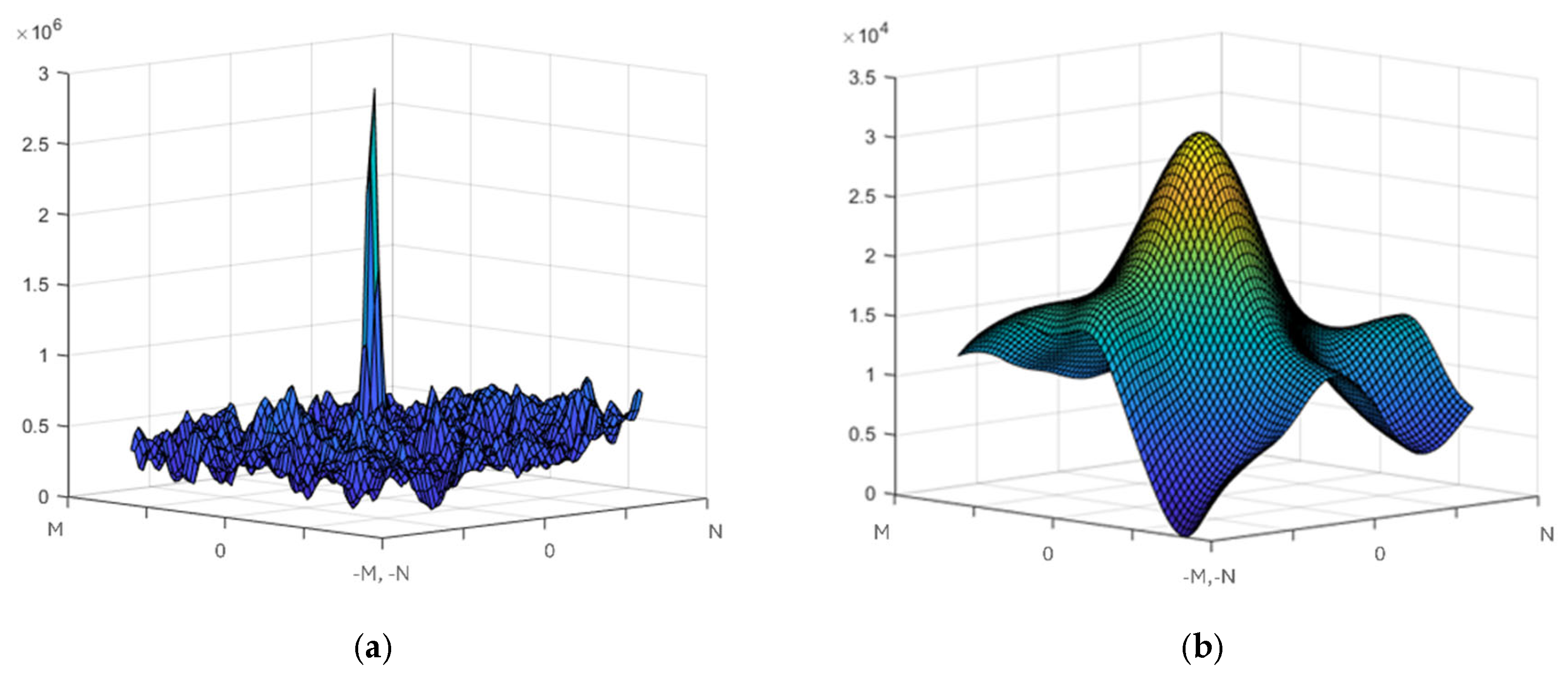
The two images $I_{1,0}$ and $I_{2,0}$ from the collected image pair are blurred using a 2-D Gaussian smoothing kernel with a standard deviation of 8 and 0 edge padding to give $I_1$ and $I_2$. This relaxation of the objective surface yields a smooth objective surface that can be relatively well defined by hyperbolic expressions. Figure 1 shows the standard objective surface often used in estimation of a velocity vector (${\left[u, v\right]}^T$) at some point (${\left[x, y\right]}^T$) (left) compared to surface generated by the proposed blurring method (right). To ensure consistency with published methods in PIV analysis, both of these surfaces were generated with the cross-correlation equation (Equation (3)) rather than the objective surface equation of the proposed method.

$$\psi \left(u,v\right)=\sum _{m=-M}^M\sum _{n=-N}^N{I}_1\left(x+m,y+n\right)\ast I_2\left(x+m+u,y+n+v\right)$$

(3)

where $\psi (u,v)$ is the cross-correlation value for a given vector displacement ($u,v$). I(x + m, y + n) is the light intensity value for the given pixel at (x + m, y + n) in the first image. The domain of consideration is centered at x, y and ranges across 2M + 1 by 2N + 1; I₂ is the intensity at the displaced second image. The candidate values of u and v range are evaluated on a domain from −M to M and −N to N.

The proposed method uses a different approach the (2M + 1) * (2N + 1) grid search for each location of interest. A grid of nine points is located around the best u and v estimates ($u^{\prime }, v^{\prime }$, respectively) on the interrogation window, defined by Equation (4). Initially, $u^{\prime }$ and $v^{\prime }$ were defined as zero, and the half-range of the initial grid (${\varphi }_b$) is defined as five pixels. ${\varphi }_b$ determines the size of the domain of nine candidate vectors that are used to characterize the objective surface across. The refining of ${\varphi }_b$ in successive iterations allows the algorithm to converge upon an optimal vector.

$$\begin{array}{c}\mathbf{g}=\left[g_1,g_2,g_3\right]=\left[-{\varphi }_b,0,{\varphi }_b\right]+u_i^{\prime }\\ \mathbf{h}=\left[h_1,h_2,h_3\right]=\left[-{\varphi }_b,0,{\varphi }_b\right]+v_i^{\prime }\end{array}$$

(4)

The u and v values of those nine points are used in Equation (7) nine times to generate the matrices defined in Equation (6). The alpha values in Equation (7) are unknowns, and will define the shape of the polynomial surface generated by Equation (5) that best matches the correlation surface created with Equation (5)

$$\begin{array}{c}\psi \left(g_k,h_l\right)={\displaystyle \sum _{m=-M}^M}{\displaystyle \sum _{n=-N}^N}{\left(I_1\left(x+m,y+n\right)-I_2\left(x+m+g_k,y+n+h_l\right)\right)}^2\\ \psi \left(g_k,h_l\right)={\alpha }_1{g}_k^2+{\alpha }_2{h}_l^2+{\alpha }_3{g}_k+{\alpha }_4{h}_l+{\alpha }_5{g}_k{h}_l+{\alpha }_6\end{array}$$

(5)

$$\begin{array}{cc}\hfill & \mathbf{A}\mathsf{\alpha }=\mathsf{\psi }\\ \mathrm{where}\hfill & \\ \hfill & \mathbf{A}=\left[\begin{array}{cccccc}{g}_1^2& h_1^2& g_1& h_1& g_1{h}_1& 1\\ g_1^2& h_2^2& g_1& h_2& g_1{h}_2& 1\\ g_1^2& h_3^2& g_1& h_3& g_1{h}_3& 1\\ g_2^2& h_1^2& g_2& h_1& g_2{h}_1& 1\\ g_2^2& h_2^2& g_2& h_2& g_2{h}_2& 1\\ g_2^2& h_3^2& g_2& h_3& g_2{h}_3& 1\\ g_3^2& h_1^2& g_3& h_1& g_3{h}_1& 1\\ g_3^2& h_2^2& g_3& h_2& g_3{h}_2& 1\\ g_3^2& h_3^2& g_3& h_3& g_3{h}_3& 1\end{array}\right];\mathsf{\alpha }=\left[\begin{array}{c}{\alpha }_1\\ {\alpha }_2\\ {\alpha }_3\\ {\alpha }_4\\ {\alpha }_5\\ {\alpha }_6\end{array}\right];\mathsf{\psi }=\left[\begin{array}{c}\psi \left(g_1,h_1\right)\\ \psi \left(g_1,h_2\right)\\ \psi \left(g_1,h_3\right)\\ \psi \left(g_2,h_1\right)\\ \psi \left(g_2,h_2\right)\\ \psi \left(g_2,h_3\right)\\ \psi \left(g_3,h_1\right)\\ \psi \left(g_3,h_2\right)\\ \psi \left(g_3,h_3\right)\end{array}\right]\end{array}$$

(6)

$$\mathsf{\alpha }={\mathbf{A}}^{-1}\mathsf{\psi }$$

(7)

Those alpha values are evaluated with Equation (7) using the inverse operation (in this paper, the MATLAB 2022b inverse operator was used). Once Equation (5) is fully defined, the minima of the surface is found with the first derivatives of the surface, Equation (8). The derivatives in Equation (8) can be set to zero to locate the minima, Equation (8). Solving the two resulting equation $\left({\displaystyle \frac{d\psi }{du}}, {\displaystyle \frac{d\psi }{dv}}\right)$, Equation (8) gives the optima u and v locations (${\left[u_{opt}, v_{opt}\right]}^T$).

$$\begin{array}{cc}\hfill & {\displaystyle \frac{d\psi }{du}}=2{\alpha }_1{u}_i+{\alpha }_3+{\alpha }_5{v}_i\\ \hfill & {\displaystyle \frac{d\psi }{dv}}=2{\alpha }_2{v}_i+{\alpha }_4+{\alpha }_5{u}_i\\ \hfill & \mathbf{P}{\left[u_{opt},v_{opt}\right]}^T=\mathbf{q}\\ \mathrm{where}\hfill & \\ \hfill & \mathbf{P}=\left[\begin{array}{cc}2{\alpha }_1& {\alpha }_5\\ {\alpha }_5& 2{\alpha }_2\end{array}\right];\mathbf{q}=\left[\begin{array}{c}{\alpha }_3\\ {\alpha }_4\end{array}\right]\\ \hfill & {\left[u_{opt},v_{opt}\right]}^T={\mathbf{P}}^{-1}\mathbf{q}\end{array}$$

(8)

As the original array of light intensity values is discretized, Equation (7) finds the closest pixel location for the minima point, and the process is repeated from Equation (4) through Equation (7) where ${\varphi }_b=3$, and a final time from Equation (4) through Equation (8) where ${\varphi }_b=1 ({\varphi }_b\in \left\{ \right\}$).

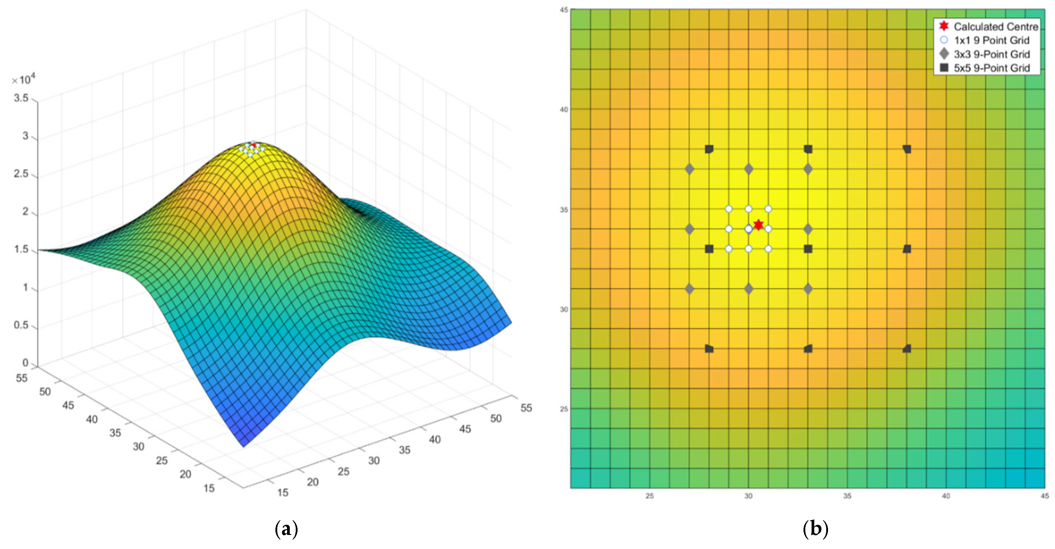
Equations (3)–(9) are repeated across $i$ = {1, 2, 3} iterations with ${\varphi }_b=5, 3, 1$, respectively. For the final iteration (${\varphi }_b=1$), Equation (9) is ignored. The locations of interest are shown for an arbitrary case in Figure 2b.

$$u_{i+1}^{\prime }=u_i^{\prime }+\mathit{round}(u_{\mathit{opt}}), v_{i+1}^{\prime }=v_i^{\prime }+\mathit{round}(v_{\mathit{opt}})$$

(9)

The final u_opt and v_opt values (depicted as the red star in Figure 2) provide the optimal shift between the two images indicating the velocity vector. The process is repeated for every location of interest to build a velocity vector field. The interrogation areas used in this implementation were 65 × 65 pixels (M = N = 32). The velocity field was identified at 12 pixel increments to generate a comprehensive velocity vector field. To avoid issues with incomplete interrogation fields, the first location of interest was located 38 pixels from the edge.

2.2. Validation of Solution on Synthetic Data

The initial validation of this method uses reference velocity vectors created with the in silico PIV-image-generation code developed by Mendes et al. [16]. The generation code outputs two PIV images based on inputs such as flow type, particle size, particle density, and velocity. The proposed method was tested with the flow type ‘Rotated Shear Flow’ which demonstrates a range of velocity magnitudes, and areas of flow that required sub-pixel accuracy to resolve. The inputs to the image-generation code are as follows: Pixel Radius = 3.0; Particle Density (Ni) = 12; Displacement Ratio (DeltaXFactor) = 0.2; Noise Level = 0; Out-of-plane standard deviation = 0.025. The velocity vectors provide a true solution to compare the results of the proposed method against. To compare the generated vectors to the reference vectors the average error per vector was found for several different particle sizes, maximum speeds and particle density. This average error per vector was taken from the total error summed from every comparison between the magnitudes of the generated and reference vectors as shown in Equation (10). The maximum relative vector error was also compared to the largest vector magnitude present in the reference vectors.

$$\mathsf{\epsilon }=\left|{\mathbf{u}}_{reference},-{\mathbf{u}}_{generated}\right|+\left|{\mathbf{v}}_{reference},-{\mathbf{v}}_{generated}\right|$$

(10)

2.3. Validation of Solution on In Vitro Data

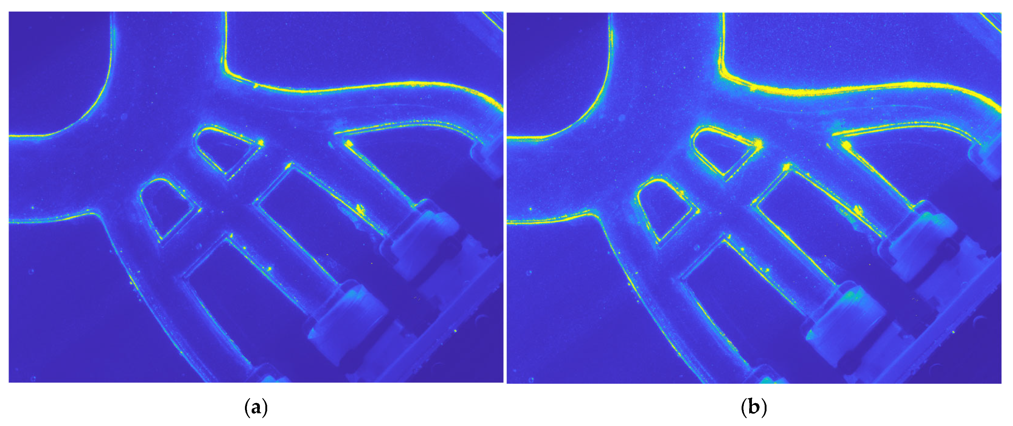
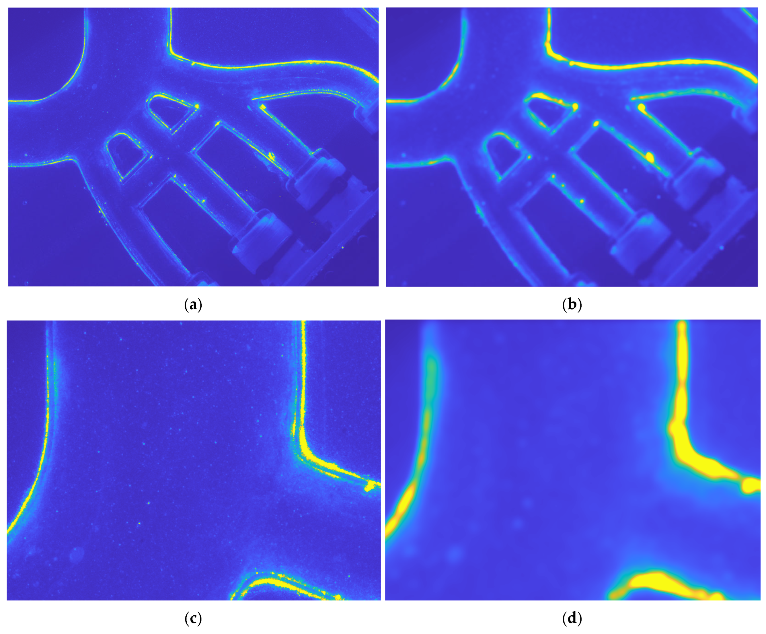
This method will also be validated on PIV image data from an experiment considering perioperative bypasses in the supra-aortic branches by Williamson et al. [17]. This experiment measured the flow in a compliant phantom of the aorta, supra-aortic arteries and their bypasses and pulsatile flow waves. The camera focus was set precisely to ensure the illuminated light sheet was in focus, and therefore there was minimal blur of the particles on the raw images. The raw image is of 1768 × 2352 pixel resolution, which allows for particles to show as an area of multiple pixels. The blur on the edge of each particle is very minimal before the preprocessing blur is applied in the polynomial method. The images used in this paper were from the peak flow of this waveform. This peak flow point was selected, as there would be strong flow signals useful for intuitive interpretation and statistical analysis. The image pair is displayed in Figure 3, with a time difference of 400 microseconds between the two image captures. Note that light refraction from the laser caused bright spots on the phantom walls.

Equations (1)–(7) were used without alteration across the in silico and in vitro datasets. Reference vectors were not available from the in vitro original experiment; however, they can be calculated using the cross-correlation method outlined above.

2.4. Processing Time Comparison Between Methods

The computer calculation time for a variety of image sizes was evaluated on an 11th Gen Intel^® Core™ i7-11700 @ 2.50 GHz with 32 GB installed RAM (HP Inc., Palo Alto, CA, USA) using Matlab 2022b. The time taken to perform the vector analysis for each method was measured using the MATLAB ‘tic-toc’ function. The difference in time between the Basic PIV method and the proposed polynomial method can be calculated and normalized by the image pixel counts that were calculated.

3. Results for the In Silico Images

3.1. Single Example Result

Figure 4 shows the initial images and the resulting vector fields from both the reference and solution methods for the Rotated Shear flow. Figure 5a shows the error magnitude. The error across y $\in$ {74, 134, 254} values is plotted in Figure 5b showing the solution vectors v component closely matches the dashed reference v component apart from the peaks of the green line and the right end of the blue line. The first row of data in

Table 1. Error results.

In Silico Settings				Approach Assessment
Flow Type	Pixel Radius [Pixels]	Pixel Density [Particles Per Interrogation Area]	Maximum Velocity in Reference [Pixel/dt]	Relative Maximum Error to Max Velocity	Average Error Per Vector [Pixel/dt]
Uniform Rankine	5.0	6	6.33	14.08%	0.208
“	2.0	5	3.17	19.20%	0.149
“	6.0	5	3.17	19.23%	0.180
“	2.0	10	3.17	17.17%	0.138
“	6.0	10	3.17	18.34%	0.160
“	2.0	5	6.33	15.29%	0.205
“	6.0	5	6.33	13.50%	0.214
“	2.0	10	6.33	19.68%	0.200
“	6.0	10	6.33	15.98%	0.241
Decaying Vortex	1.5	12	4.80	14.03%	0.209
Stagnation	4.0	8	5.78	8.18%	0.164
Parabolic	3.0	8	4.00	10.42%	0.122
Rotated Shear	5.0	5	5.87	9.14%	0.140

shows the summary statistics for this flow type.

3.2. Error over Multiple Examples

Using the error measurements from Equation (8), the solution method was performed on a range of particle radius and particle densities, and a selection of different flow types. Table 1 displays the input variables and error results, where the first line is from the image pair analyzed in Figure 4 and Figure 5.

3.3. Processing Speed Comparison Between the Original and Proposed Method

These results were found using the two methods performed on the Uniform Rankine flow type with pixel radius 5.0 and a Pixel Density of 6. The Speed Ratio value increases as the original image size increases. This demonstrates the difference in time between the Basic and Polynomial Proposed methods does not increase linearly with respect to the image size increase.

4. In Vitro Image Results

The blurred image is shown in Figure 6, with comparison to the unblurred image, and a zoomed in area of the flow path below. The code was run, and produced these vector fields in Figure 7. For clarity, Figure 7b shows the same outcome with all vectors over 15 pixels in magnitude removed.

Additionally, the code was run on the isolated section shown in Figure 6d to determine how it performs when not facing any effect from the wall brightness. The results of this, compared to the original cross-correlation method are shown in Figure 8.

It is clear the proposed approach failed to capture an accurate velocity vector field in the in vitro dataset. The coherence of the flow indicated by the traditional method [17] indicates that the problem was not with the data itself. Rather, the proposed method failed to properly identify the vectors from the data. The incoherence of the resultant vectors precludes further statistical analysis.

5. Discussion of In Silico Data Results

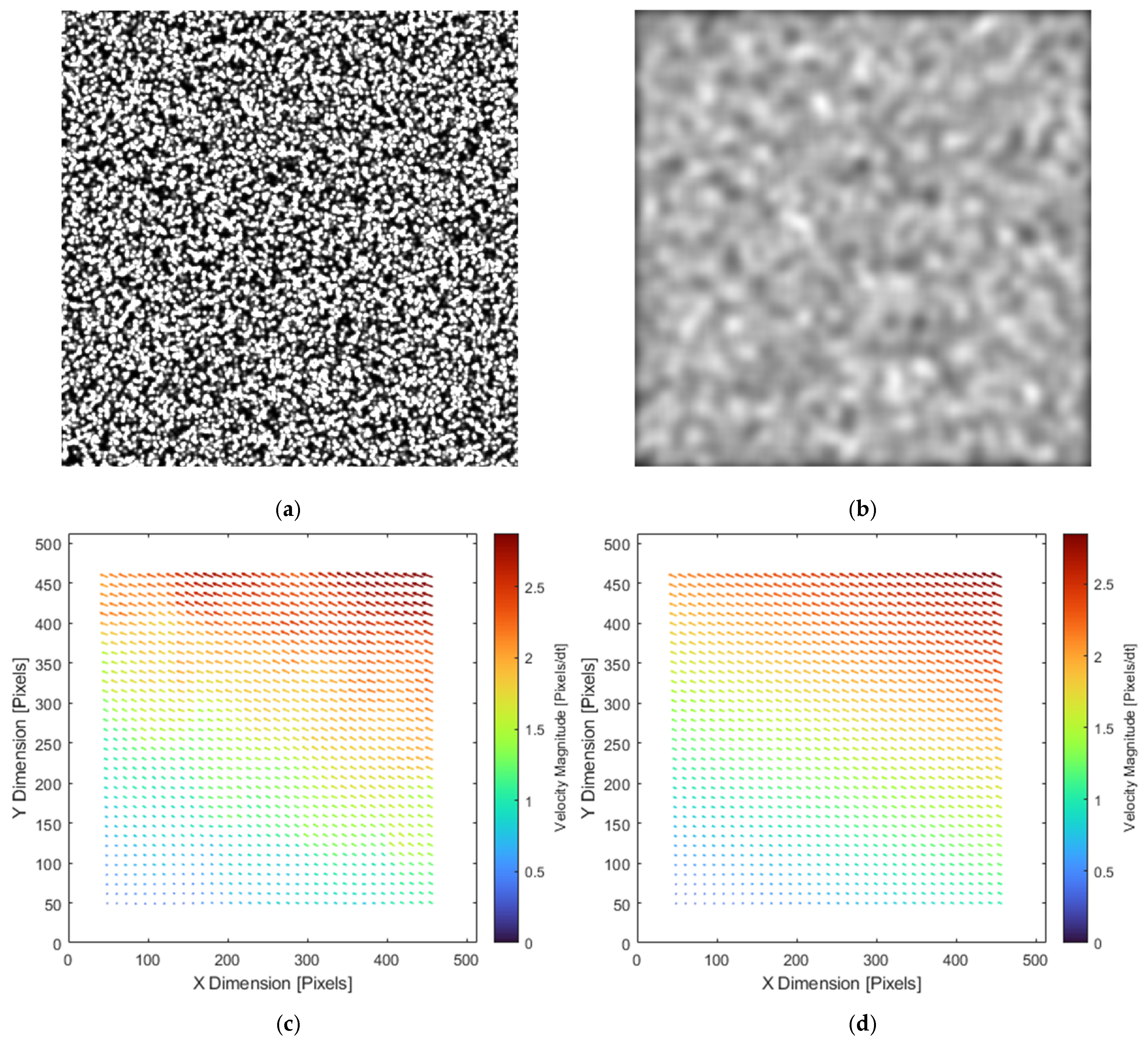
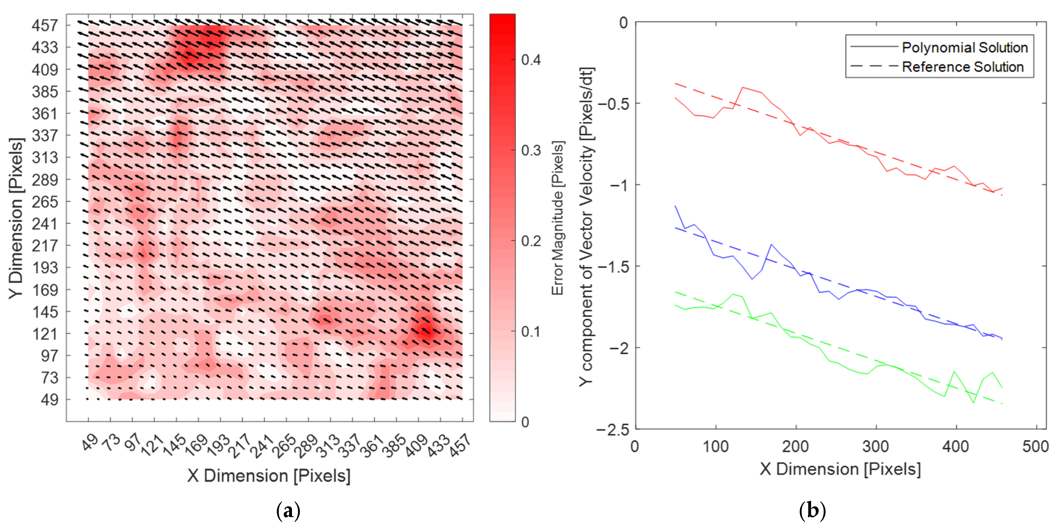
The in silico results (Figure 4 and Figure 5, Table 1) indicated the proposed method was promising. The velocity vector fields generated by the polynomial approximation method look very similar to the reference velocity fields (Figure 4c,d). There was a low level of error in the vector field in a variety of flow cases (Table 1). For context, competitors in the PIV challenge reported errors in the range of 2–6 pixel magnitudes for a similar problem using a Rankine Vortex flow [18]. The proposed approach was robust to changes in the image generation code as the particle size and density was varied. This demonstrated the method’s potential across a wide range of PIV situations. The maximum error percentage stayed under 20% for every case displayed in Table 1 and under an average of 0.25 pixel/dt per vector.

This low average error rate shows an improvement over methods that do not determine the sub-pixel cross-correlation peak. Methods that do not optimize to the subpixel scale have a minimum average expected error of 0.383 (based on ${\int }_{-0.5}^{0.5}{{\int }_{-0.5}^{0.5}‖x,y‖}_{2}dxdy$). The lowest error for the proposed method occurred in the parabolic test case with small particles, moderate density and lower maximum velocity with an average error per vector of only 0.122 pixels. The accuracy which exceeds the theoretical maximum accuracy is due to the smoothing effects of the approach effectively capturing flow-vector coherence information from not just the optimal vector, but also from vectors close to the optimal vector. Furthermore, the appearance of PIV particles in discrete pixel-space does not necessarily preserve the pixel shape for a particle across image pairs. Hence, the relaxation (or convolution) phase of the proposed approach ultimately leads to a smoother objective surface that is more coherently observed by the optimization process.

The particularly strong performance in the ‘parabolic’ case was somewhat expected, as the parabolic flow type only has horizontal flow that changes magnitude depending on the y value. The solution with the lowest relative error was the ‘stagnation flow’ case with medium particle size, moderate density, and high maximum velocity (however, this had a higher average error per vector than the parabolic flow). Both of these cases had flow in only one orthogonal direction. When the particles are moving uniformly in one direction, the vector has only one component, so the potential for error is reduced. The largest relative error occurred in the Uniform Rankine flow with small particles, high density, and high maximum velocity. This error behavior was expected, as a Rankine vortex has a sharp change in flow velocity at the horizon radius, which physical flow situations cannot experience due to the coherence between fluid layers.

The worst errors were in the velocity transition zones near the Rankine vortex horizon. The in silico simulation of the Rankine vortex had a sharp change in velocity profile, which is not typical in subsonic flows. Thus, any peak within the interrogation window is ultimately smoothed off. However, this error is common to most PIV approaches as velocity is typically assumed constant across the interrogation window. Nonetheless, increased camera resolution and a higher seeding-particle density would allow a smaller interrogation region and thus smaller averaging error.

The proposed method only needs to calculate 27 correlation values to find the optimum displacement position. This is significantly less than the typical (2M + 1) * (2N + 1) exhaustive search. The results from

Table 2. Processing Time Comparison.

Image Dimensions (Pixels)	Basic PIV Method Speed [s]	Proposed Polynomial Method Speed [s]	Difference in Time (Δt) [s]	Total Pixels in Image	$\mathbf{Speed} \mathbf{Ratio} \frac{∆\mathit{t}}{\mathit{M}\ast \mathit{N}}$
512 × 512	0.912	0.740	0.172	0.262 × 106	0.656 × 10−6
1766 × 2352	22.3	17.0	5.30	4.15 × 106	1.27 × 10−6
7072 × 9408	494	281	213	66.5 × 106	3.20 × 10−6

with the processing time calculations show this difference in computational burden has a demonstrable effect. Other methods, including those used by OpenPIV and PIVlab, perform an entire field cross-correlation before using a Gaussian-fit method to get the subpixel accuracy. This approach is computationally expensive for large interrogation windows, as the number of entries needing to be calculated in the correlation matrix is a 4:1 ratio of the number of pixels in the interrogation window. The proposed method bypasses the unnecessary calculations from {u, v} values, which, after some preliminary calculations, are highly unlikely to contain the optima. By measuring the performance on the course 3 × 3 grid of nine points, then refining the grid size and reevaluating, the proposed approach is similar to a bisection method. This approach is only achievable due to the Gaussian smoothing of the original pictures. This smoothing allows locations proximal to the optima to have a moderate correlation score. This allows convergence to the optimal value. In contrast, when only points in space are illuminated, locations proximal to the optimum will have a low correlation, and an exhaustive search is necessary. When the image size increased, the speed ratio also increased. This indicates that the proposed polynomial method gets faster in comparison to the basic PIV method [19] when the image size is increased, and is still faster in the smaller images.

The validation process used when evaluating this proposed polynomial approach also has some limitations. Some of the aspects of in vitro data that were not included in this experiment were background noise from the material behind the experiment phantom, difference in contrast between images due to the laser pulse timing, out-of-plane motion or artifacts from either the camera, or flaws in the experiment materials. None of this is captured in the in silico data. Thus, the proposed approach was not validated with respect to these known effects. Nonetheless, this preliminary in silico analysis was undertaken to evaluate the approach with a known true value to compare the optimization against. This direct comparison allowed a direct validation against known values rather than the axiomatic validation of using in vitro data. The images were generated from exact equations, and thus the reference vectors could be found directly from these equations. The majority PIV work is applied to in vitro flows. However, the accuracy of a proposed method is much harder to evaluate statistically when applied to data that lacks a known perfect solution. The behavior of the in vitro flow can be theorized based on the experiment set-up and previous published work on the flow characteristics but there will not be a perfect reference to evaluate against.

6. Discussion of In Vitro Results

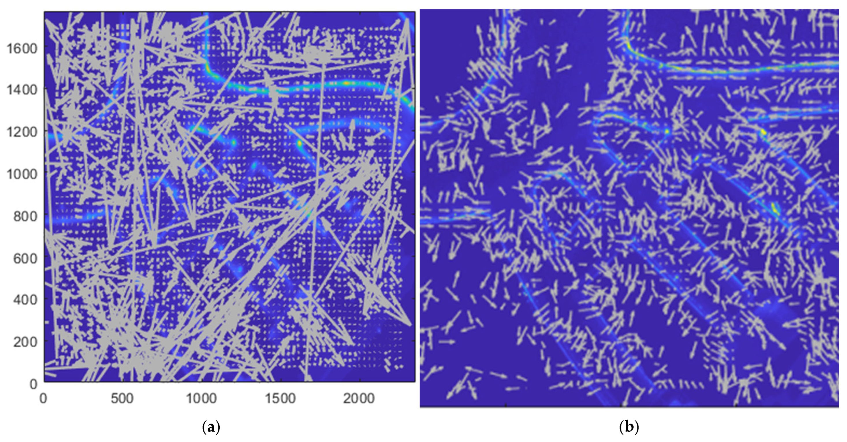
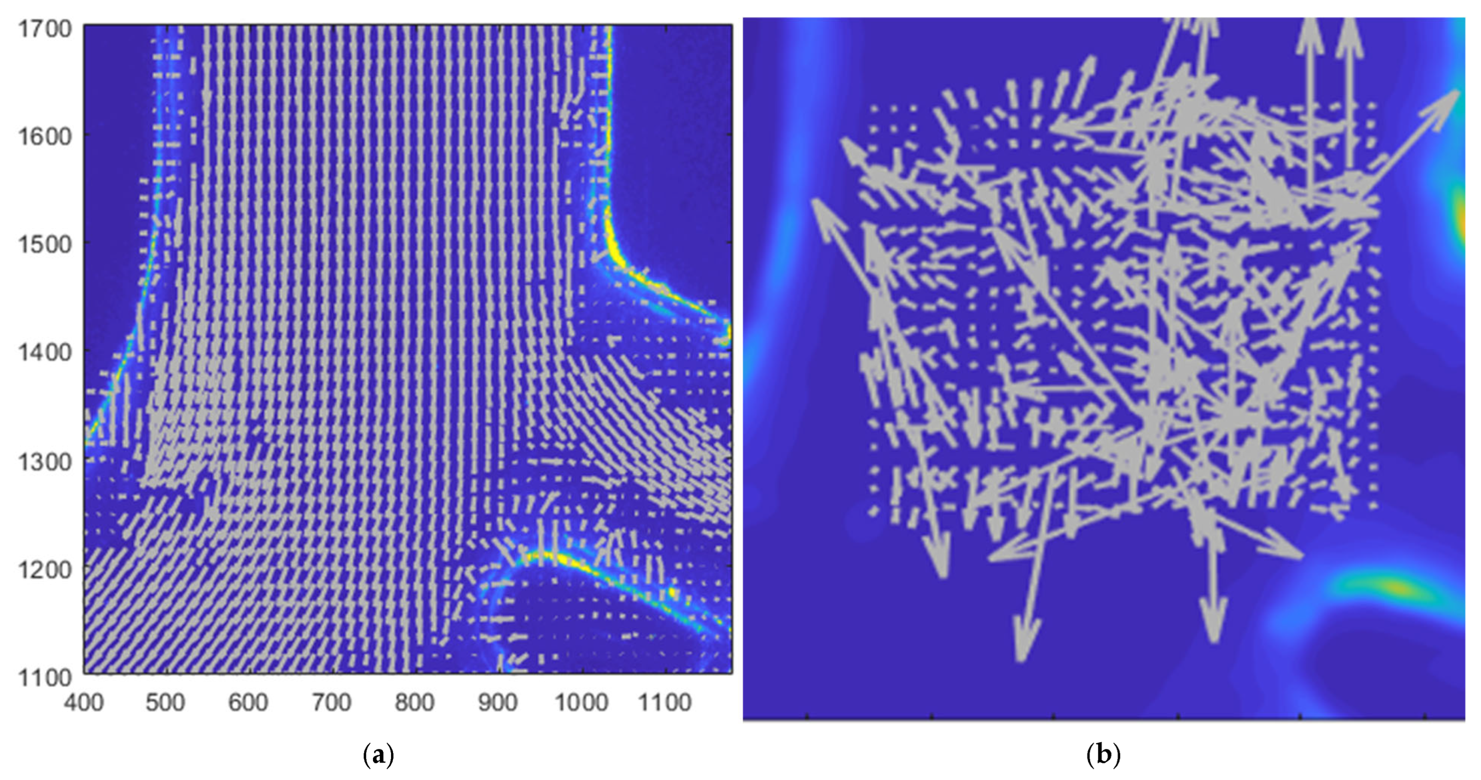
The proposed method was proven to be efficient and effective when applied to PIV data that was generated in silico. However, the proposed method yielded unusable, incoherent images when applied to the in vitro PIV images (Figure 7). The traditional method was successful in the in vitro data (Williamson et al. [17]) and exhibited coherent image reconstruction using the same data (Figure 7). A large portion of the vectors in the in silico data are above 15 pixels in magnitude, which is equivalent to 2.25 ms⁻¹. The known velocity was in the region of 0.1 to 0.5 ms⁻¹, which is shown in the findings of Williamson et al. [17]. That velocity equates to a pixel offset of approximately one to four pixels between image pairs, and was well within the accepted recommendation of pixel offsets no more than 1/4th the size of the interrogation window [20] of 32 pixels by 32 pixels. This pixel offset would have been within the $-5\to +5$ pixel bounds of the proposed methods. The consistently erratic vector directions and magnitudes indicate an absolute failure in the method. As the haemodynamics this in vitro experiment is mimicking are through cylindrical smooth geometry with simple boundary conditions, the flow vector field is expected to be coherent with no discontinuities. This is because the flow must adhere to the Navier–Stokes equations [21], and at the Reynolds Number calculated for this in vitro example [17] the flow is expected to be laminar [22]. The incoherence of the flow profiles generated by the proposed method imply that statistical analysis is superfluous.

As Figure 6 shows, the wall imperfections dominate, as they are much brighter than the areas around them, and the zoom in section in (Figure 6c) displays how much brighter the wall is than the particles in the flow space. After blurring, these particles lose light intensity and noise in the background is amplified. While this issue could be mitigated by masking the wall regions, incoherent vector estimations were observed in regions distant from the walls (Figure 7 and Figure 8). These results mean the approach, which was validated in in silico data, was not valid for use in in vitro data.

To attempt to overcome the issues with the application of the method to the real data, a number of preprocessing methods were applied to the in vitro data images. These included applying scaling curves to ensure light-intensity matching across image pairs and transforming the images using sigmoidal functions that amplify particles and mitigate the lightness where there were no pixels apparent, and thresholding. However, none of the preprocessing methods yielded suitable velocity vectors.

While the in vitro results were disappointing and indicate the approach is not currently fit for our purpose, there is excellent performance of the approach in in silico data as well as apparent, and theoretically justifiable, consistent improvement of the theoretical limit of precision. The authors feel this implies that it is suitable for presentation to the academic community. Despite the initial success of the in silico results it was important to consider in vitro testing. PIV is a useful tool for validating computational fluid dynamic models or to capture flow with complex fluid to solid interactions. This is why testing and reporting on the proposed approach with PIV data was important.

Future work to improve this method for use in PIV experimental image processing seems possible if the right prepossessing is determined. However, such an augmentation will alter the in vitro image characteristics to conform to the characteristics of the in silico data and therefore could negate the savings in time and computational load.

7. Conclusions

While there has been stagnation in the development of new PIV image analysis methods in recent decades, the proposed approach described in this paper shows there is still potential to progress the field. To the authors’ knowledge, the proposed approach is a novel concept that utilizes image blurring to allow smoother objective surfaces that conform to second-order parabolic functions local to the optima point, especially in in silico-generated data. The low relative errors over a large variety of flow types, particle sizes, and densities demonstrate the flexibility and precision of the method. However, the proposed method was unable to find a coherent vector field for the in vitro images. Nonetheless, the proposed method is novel and solved a particular problem very quickly and with high accuracy. Hence, it may be suitable for a class of image analysis tasks outside the PIV field.