Three-Dimensional CFD Simulations of the Flow Around an Infinitely Long Cylinder from Subcritical to Postcritical Reynolds Regimes Using DES

Abstract

The flow around circular cylinders is a classic problem in fluid mechanics with significant implications for offshore engineering. While extensive numerical and experimental research has focused on the subcritical and critical Reynolds regimes, the supercritical and postcritical regimes remain challenging and relatively unexplored, primarily due to the complex nature of turbulence and the high computational requirements. In this study, we perform three-dimensional detached eddy simulations using the finite volume method in OpenFOAM v1906, employing Menter’s k-$\omega$ SST turbulence model, to systematically investigate the flow past an infinitely long smooth cylinder from the subcritical through the postcritical regimes. The numerical setup ensures accurate near-wall resolution and reliable representation of unsteady flow features. We present a detailed analysis of vortex shedding patterns, wake evolution, and statistical properties of lift and drag coefficients for selected Reynolds numbers representative of each regime. The simulation results are benchmarked against experimental data from the literature, demonstrating good agreement for Strouhal number and mean drag. Special emphasis is placed on the evolution of wake topology and force coefficients as the flow transitions from laminar to fully turbulent conditions. The findings contribute to the limited numerical literature on flow around circular cylinders across subcritical, critical, supercritical, and postcritical Reynolds number regimes, providing insights that are fundamentally relevant to the broader scope of understanding vortex shedding phenomena.

1. Introduction

The study of fluid flow around circular cylinders is a cornerstone in fluid mechanics, driven by both its practical relevance to engineering systems and the fundamental insights it provides into complex flow phenomena. This type of flow behavior is present in many applications, such as bridge piers, offshore structures, heat exchangers, and aerospace components. The classification of regimes in the flow around a circular cylinder is usually based on the nature of the boundary layer, which may be laminar, transitional, or turbulent, and is directly related to the Reynolds number ($Re$) of the flow. For a smooth cylinder, the transition from the subcritical to the critical regime occurs at a Reynolds number of approximately $2.8\times {10}^5$. Below this value, the boundary layer remains laminar up to separation, which leads to periodic vortex shedding and a characteristic Strouhal number close to 0.2 [1,2,3]. The classical nature of this problem makes it a reference case for both experimental and computational studies on bluff body flows.

According to Zdravkovich [4] and Roshko [5], the critical regime for the flow over a circular cylinder extends from $\mathit{Re}=1.4\times {10}^5$ to $\mathit{Re}=1\times {10}^6$. The transition from the supercritical to the postcritical regime is marked by the transcritical regime, which occurs within the range $\mathit{Re}=1\times {10}^6$ to $\mathit{Re}=3.5\times {10}^6$. The postcritical regime, defined by $\mathit{Re}>8\times {10}^6$, is considered the final stage of flow development [4]. These higher-Reynolds-number regimes are commonly encountered in large-scale offshore structures, including wind turbine towers, oil and gas platforms, and risers [6]. In such environments, the structural elements are exposed to the combined action of ocean currents and wind, resulting in a complex setting where the interaction between the fluid and the structure is governed by nonlinear effects [7].

From the perspective of fluid dynamics, the incompressible flow around a circular cylinder represents a significant challenge, both theoretically and experimentally [4]. As the Reynolds number increases, the complexity of the flow structures and the physical mechanisms involved also increases. For example, the drag coefficient deviates from its subcritical value in the critical regime, indicating the onset of the drag crisis as the separation point shifts downstream and the drag is significantly reduced [8]. Simultaneously, the wake narrows and the Strouhal number rises, reaching values as high as 0.33 in the critical regime. A steady mean lift force may also develop due to asymmetries in the flow, resulting in a bistable pattern associated with the transition of the boundary layer between laminar and turbulent states and the appearance of random lift fluctuations. The minimum drag coefficient observed in the critical regime is a key marker, and the end of this regime is characterized by the formation of separation bubbles on both sides of the cylinder. When the supercritical regime is reached, these bubbles become stable and periodic vortex shedding resumes, with Strouhal numbers as high as 0.48 [9].

The transcritical regime is distinguished by the disruption and fragmentation of separation bubbles along the span of the cylinder, producing an irregular separation line [4]. In this upper transitional range, the disappearance of the separation bubble and the establishment of relatively stable turbulent separation points signal the reappearance of periodic vortex shedding [4,9]. Finally, the postcritical regime is attained when the free shear layers, wake, and boundary layers are fully turbulent. Although no additional regime transitions are expected beyond the postcritical state, the flow remains sensitive to further increases in Reynolds number. This leads to continued thinning of the boundary and shear layers, which can alter the separation point location and thus affect both the width of the near wake and the Strouhal number [4].

One of the persistent challenges in the study of high-Reynolds-number flows around cylinders is the accurate experimental measurement of turbulent and three-dimensional flow structures. Also, in numerical simulations at such regimes, substantial computational resources are required because of the need for fine grids, small time steps, and robust numerical algorithms to solve the details of the flow [10]. As a result, despite the importance of these flows for engineering applications, the supercritical and postcritical regimes remain insufficiently explored, both in terms of experimental data [5,11] and high-fidelity numerical simulations [12,13]. For high Reynolds numbers, detailed information on the effects of Reynolds number on the flow features of circular cylinders is especially difficult to obtain experimentally [4,9]. Recent studies confirm that in the postcritical regime the drag coefficient becomes nearly insensitive to Reynolds number, highlighting the scarcity of reliable experimental measurements in this range [14].

Given this context, the main objective of the present work is to address these gaps by estimating the unsteady loads acting on a circular cylinder, including lift, drag, and pressure coefficients, as the flow transitions from the subcritical to the postcritical regime. Using a robust Computational Fluid Dynamics methodology based on the Finite Volume Method implemented in OpenFOAM v1906, the present study analyzes the flow at Reynolds numbers of $5\times {10}^4$, $1\times {10}^5$, $5\times {10}^5$, $1\times {10}^6$, $3.6\times {10}^6$, and $1\times {10}^7$. Flow structures are characterized in terms of instantaneous iso-contours of normal vorticity and three-dimensional perspectives of Q criterion isosurfaces colored by vorticity magnitude.

2. Methodology

The CFD modeling developed in this work employs the Detached Eddy Simulation (DES) approach with the k-$\omega$ SST turbulence model, which has been widely used and validated for bluff body flows at high Reynolds numbers due to its ability to handle flow separation and adverse pressure gradients [15,16,17]. The primary advantage of the DES approach is its ability to combine the robust near-wall modeling of URANS (k-$\omega$ SST) with the explicit resolution of large-scale, three-dimensional turbulent structures in the wake via LES. This hybrid character is particularly important in the supercritical and postcritical regimes, where both accurate near-wall treatment and computational efficiency are critical for reliable simulations. The near-wall region is modeled using wall functions, and mesh refinement strategies are applied to ensure accurate resolution of the boundary layer, following established recommendations [18]. Numerical simulations were carried out for three Reynolds numbers, $5\times {10}^4$, $1\times {10}^5$, and $5\times {10}^5$, corresponding to the subcritical, transitional, and critical regimes. Results for higher Reynolds numbers, $1\times {10}^6$, $3.6\times {10}^6$, and $1\times {10}^7$, associated with the supercritical, transcritical, and postcritical regimes, were obtained in a previous study by some of the authors of this paper and reported in [19]. By combining the new simulations with the analyses already established in that earlier work, it is possible to provide a unified discussion encompassing the subcritical, transitional, critical, supercritical, transcritical, and postcritical regimes, in agreement with the classifications discussed by Zdravkovich [4,20] and Niemann & Hölscher [9]. For all simulations, the Courant–Friedrichs–Lewy (CFL) number was fixed at 1 to ensure numerical stability and consistency. Additional information on temporal discretization sensitivity for unsteady loading in circular cylinders at high Reynolds numbers is available in de Oliveira et al. [19].

2.1. Governing Equations

The fluid dynamics of the flow around a circular cylinder are modeled as three-dimensional, transient, turbulent, and incompressible. To facilitate numerical modeling, the flow variables are decomposed according to Reynolds averaging, whereby any instantaneous quantity $\varphi$ (such as velocity or pressure) is expressed as the sum of a time-averaged component $\overline{\varphi }$ and a fluctuating part ${\varphi }^{\prime }$, as shown below:

$$\varphi =\overline{\varphi }+{\varphi }^{\prime }.$$

(1)

Applying this decomposition to the Navier–Stokes equations results in the unsteady Reynolds-averaged Navier–Stokes (URANS) equations, which govern the conservation of mass and momentum for the mean flow:

$$\begin{array}{c}{\displaystyle \frac{𝜕{\overline{u}}_j}{𝜕x_j}}=0,\end{array}$$

(2)

$$\begin{array}{c}\rho {\displaystyle \frac{𝜕\left({\overline{u}}_i\right)}{𝜕t}}+\rho {\displaystyle \frac{𝜕\left({\overline{u}}_j{\overline{u}}_i\right)}{𝜕x_j}}=-{\displaystyle \frac{𝜕\overline{p}}{𝜕x_i}}+{\displaystyle \frac{𝜕}{𝜕x_j}}\left(\mu {\displaystyle \frac{𝜕{\overline{u}}_i}{𝜕x_j}}-\rho \overline{u_i^{\prime }{u}_j^{\prime }}\right),\end{array}$$

(3)

where ${\overline{u}}_i$ and ${\overline{u}}_j$ are the averaged velocity components in the i and j spatial directions, $x_j$ denotes spatial coordinates, $\rho$ is the fluid density, $\mu$ is the dynamic viscosity, and $\overline{p}$ is the mean pressure field. The terms $\overline{u_i^{\prime }{u}_j^{\prime }}$ represent the Reynolds stresses, which encapsulate the effects of turbulent velocity fluctuations on the mean flow and are essential to close the system of equations [21,22].

To express the Reynolds stresses in terms of known quantities, the Boussinesq hypothesis is typically adopted, relating these stresses to the mean rate of strain through the turbulent or eddy viscosity, ${\nu }_t$:

$$-\overline{u_i^{\prime }{u}_j^{\prime }}=-{\delta }_{ij}{\displaystyle \frac{2}{3}}k+{\nu }_t\left({\displaystyle \frac{𝜕{\overline{u}}_i}{𝜕x_j}}+{\displaystyle \frac{𝜕{\overline{u}}_j}{𝜕x_i}}\right),$$

(4)

where ${\delta }_{ij}$ is the Kronecker delta, $k={\displaystyle \frac{1}{2}}\overline{u_k^{\prime }{u}_k^{\prime }}$ is the turbulent kinetic energy, and ${\nu }_t$ is the turbulent (eddy) viscosity. The challenge of appropriately modeling the Reynolds stresses is known as the turbulence closure problem, and it motivates the development of various turbulence models [21,23].

Among the closure strategies, the Boussinesq hypothesis remains the basis for most widely used eddy-viscosity models. While this approach has limitations, particularly for complex, anisotropic turbulence, it enables practical application of two-equation models such as k-$ϵ$ and k-$\omega$ for a broad range of turbulent flows [15,23,24].

In the present study, the k-$\omega$ shear stress transport (SST) model developed by Menter [15] is adopted for the URANS component of the DES method, given its strong performance for flows with separation and adverse pressure gradients, which are characteristic of the flow around bluff bodies [15,16,20]. The governing equations for k (turbulent kinetic energy) and $\omega$ (specific dissipation rate) are

$$\begin{array}{c}{\displaystyle \frac{𝜕k}{𝜕t}}+{\displaystyle \frac{𝜕\left({\overline{u}}_{j}k\right)}{𝜕x_j}}= {\displaystyle \frac{𝜕}{𝜕x_j}}\left[(\nu +{\sigma }_k{\nu }_t){\displaystyle \frac{𝜕k}{𝜕x_j}}\right]+\tilde{P}k-{\beta }^{*}k\omega ,\end{array}$$

(5)

$$\begin{array}{c}{\displaystyle \frac{𝜕\omega }{𝜕t}}+{\displaystyle \frac{𝜕\left({\overline{u}}_j\omega \right)}{𝜕x_j}}= {\displaystyle \frac{𝜕}{𝜕x_j}}\left[(\nu +{\sigma }_{\omega }{\nu }_t){\displaystyle \frac{𝜕\omega }{𝜕x_j}}\right]+{\displaystyle \frac{\gamma }{{\nu }_t}}\tilde{P}k-\beta {\omega }^2+2(1-F_1){\displaystyle \frac{1}{\omega }}{\sigma }_{w_2}{\displaystyle \frac{𝜕k}{𝜕x_j}}{\displaystyle \frac{𝜕\omega }{𝜕x_j}},\end{array}$$

(6)

where $\nu$ is the kinematic viscosity, ${\sigma }_k$ and ${\sigma }_{\omega }$ are model constants, $\tilde{P}k$ denotes the limited production of k, ${\beta }^{*}$ and $\beta$ are empirical constants, $F_1$ is the blending function for the SST model, $\gamma$ and ${\sigma }_{w_2}$ are additional model coefficients, $x_j$ is the spatial coordinate, and t is time. Further details on the constants and their calibration can be found in Menter [25] and Wilcox [23].

For the Detached Eddy Simulation (DES) modification, the model dynamically switches between RANS and LES behavior by substituting the turbulence length scale $l_{k,\omega }$ with a hybrid length scale $\tilde{l}$, which incorporates the local grid size.

$$\begin{array}{c}\hfill \hspace{1em}\hspace{1em}\hspace{1em}\hspace{1em}\tilde{l}=min(l_{k,\omega },C_{\mathrm{DES}}{\Delta }_{\mathrm{DES}}),\end{array}$$

(7)

$$\begin{array}{cc}\hfill {\Delta }_{\mathrm{DES}}& =max({\delta }_x,{\delta }_y,{\delta }_z),\hfill \end{array}$$

(8)

where $l_{k,\omega }=k^{1/2}/\left({\beta }^{*}\omega \right)$, $C_{\mathrm{DES}}$ is a model constant, and ${\Delta }_{\mathrm{DES}}$ is the maximum local mesh spacing, with ${\delta }_x$, ${\delta }_y$, and ${\delta }_z$ representing the grid cell dimensions in each Cartesian direction. The value of $C_{\mathrm{DES}}$ depends on the turbulence model and is interpolated using the blending function $F_1$ as

$$C_{\mathrm{DES}-\mathrm{SST}}=(1-F_1)C_{\mathrm{DES}}^{k-ϵ}+F_1{C}_{\mathrm{DES}}^{k-\omega },$$

(9)

where $C_{\mathrm{DES}}^{k-\omega }=0.78$ and $C_{\mathrm{DES}}^{k-ϵ}=0.61$. Here, $d_w$ denotes the distance from the cell center to the nearest wall. When $\tilde{l}$ is comparable to $d_w$, the model operates in URANS mode; otherwise, in regions farther from the wall, the DES model transitions to an LES-like mode, enabling resolution of large-scale turbulent eddies [17,26].

2.2. Spatial Discretization Schemes

The spatial discretization of the governing equations is accomplished using the finite volume method (FVM), which integrates the equations over each control volume in the computational mesh. This approach ensures conservation of mass, momentum, and turbulence quantities across the computational domain [22,27].

In OpenFOAM, different discretization schemes can be applied to the convective and diffusive terms of each equation. The choice of scheme impacts both solution accuracy and numerical stability, especially in turbulent, high-Reynolds-number flows. Following the best practices for discretizing turbulent flows in complex geometries [28], the convective term of the momentum equation in the DES simulations was discretized using the Linear-Upwind Stabilized Transport (LUST) scheme, as proposed by Weller et al. [29]. This approach blends central differencing with a linear upwind scheme, providing a compromise between numerical accuracy and stability. In the present work, a blending factor of 0.25 was adopted, resulting in face values composed of 75% central differencing and 25% linear upwind, consistent with the recommendations of Jasak et al. [30]. For the turbulence transport equations of k and $\omega$, the convective terms were discretized using a second-order upwind scheme. For the remaining operators, gradients were computed using the Gauss linear scheme with linear interpolation, while Laplacian terms were discretized with central differences, following the practices recommended by Ferziger et al. [22]. Further details regarding the application of the LUST scheme in similar DES studies can be found in [31]. For the divergence terms, a second-order upwind scheme was applied, gradients were computed using the Gauss linear scheme with linear interpolation, and Laplacian terms were discretized with central differences, as also supported by Ferziger et al. [22]. The resulting linear systems were solved using the geometric-algebraic multi-grid (GAMG) method for symmetric matrices, while the preconditioned bi-conjugate gradient (PBiCG) solver with DILU preconditioner was used for non-symmetric systems, ensuring robust and scalable solutions for large CFD problems.

2.3. Temporal Discretization Schemes

The unsteady terms in the governing equations were discretized using an implicit, second-order accurate backward differencing scheme (backward Euler). This method, implemented in OpenFOAM as the “backward” scheme, was favored for its numerical stability and ability to handle stiff problems in transient turbulent flows [27,28].

The stability of the time integration is governed by the Courant–Friedrichs–Lewy (CFL) condition, which links the time step size to the mesh spacing and local velocity. The Courant number ($Co$) is defined as

$$Co={\displaystyle \frac{U_f\Delta t}{\left|\mathbf{d}\right|}},$$

(10)

where $U_f$ is the flow speed at the face of each control volume, $\Delta t$ is the time step, and $\left|\mathbf{d}\right|$ is the distance between the centers of adjacent cells. To ensure numerical convergence and accuracy in transient simulations, the Courant number is typically restricted to $Co\le 1$ for implicit schemes [27,28]. The backward differencing approach is unconditionally stable for linear problems and robust for the non-linear systems encountered in DES and URANS simulations, making it suitable for high-Reynolds-number flows [28,30].

2.4. Turbulence Modeling in the Near-Wall Region

The near-wall region is critical for capturing the dynamics of boundary layer development and separation, especially in flows over smooth cylinders [18,21]. To ensure that wall effects are accurately represented, the computational mesh was refined near the cylinder so that the dimensionless wall distance, $y^{+}$, was within the range recommended for wall function use. The $y^{+}$ parameter is defined as $y^{+}=u_{\tau }y/\nu$, where $u_{\tau }$ is the friction velocity, y is the distance from the wall, and $\nu$ is the kinematic viscosity. In OpenFOAM, wall functions are implemented following the approach described in [32], and a threshold $y_{\mathrm{lam}}^{+}$ is computed as:

$$y_{\mathrm{lam}}^{+}={\displaystyle \frac{\log \left(\max \left(E{y}^{+},1\right)\right)}{\kappa }},$$

where E is typically set to $9.8$ for hydraulically smooth walls and $\kappa$ is the von Kármán constant (0.41). This method allows the solver to distinguish between the viscous sublayer, buffer layer, and fully turbulent region, applying the appropriate model for each zone. Further details regarding the near-wall modeling approach can be found in [33].

3. Numerical Simulations

As extensively reported in the literature, the flow around a circular cylinder has been the subject of substantial experimental and numerical investigation due to its canonical importance in fluid mechanics and its direct relevance to a wide range of engineering applications [1,34]. Beyond its fundamental role in elucidating bluff-body aerodynamics, the cylinder wake provides a rigorous benchmark for assessing turbulence models and numerical strategies.

In the present study, CFD simulations were conducted to investigate the flow characteristics over a wide range of Reynolds numbers, specifically at $\mathit{Re}=5\times {10}^4$, $1\times {10}^5$, $5\times {10}^5$, $1\times {10}^6$, $3.6\times {10}^6$, and $1\times {10}^7$. These values were selected to cover the transition from the subcritical to the postcritical regime, where distinct wake dynamics and load fluctuations are observed. Flow structures were analyzed using instantaneous iso-contours of the normal vorticity field and three-dimensional visualizations of Q-criterion isosurfaces, colored by the vorticity magnitude, in order to capture coherent vortical structures across a range of scales. The Q-criterion, which is defined as the second invariant of the velocity gradient tensor ($Q={\displaystyle \frac{1}{2}}{\left(\right|\Omega |}^2-{\left|S\right|}^2)$, where $\Omega$ and S are the antisymmetric and symmetric parts of the velocity gradient, respectively), provides a robust measure for identifying vortex-dominated regions and distinguishing them from shear-dominated areas. This approach allows the primary features of the wake dynamics to be visualized in detail.

The investigations focused on the unsteady hydrodynamic loads acting on an infinitely long circular cylinder, expressed in terms of lift, drag, and pressure coefficients. The numerical model was based on a smooth three-dimensional cylinder with an aspect ratio of $l/D=2$, subject to periodic boundary conditions in the spanwise direction. To adequately capture the complex unsteady dynamics, the simulations employed a two-equation Detached Eddy Simulation (DES) turbulence model, which has proven effective in resolving large-scale unsteadiness while retaining RANS-type near-wall treatment [17,35].

The present section provides details of the computational setup and the parameters employed in the numerical investigations.

3.1. Computational Domain and Boundary Conditions

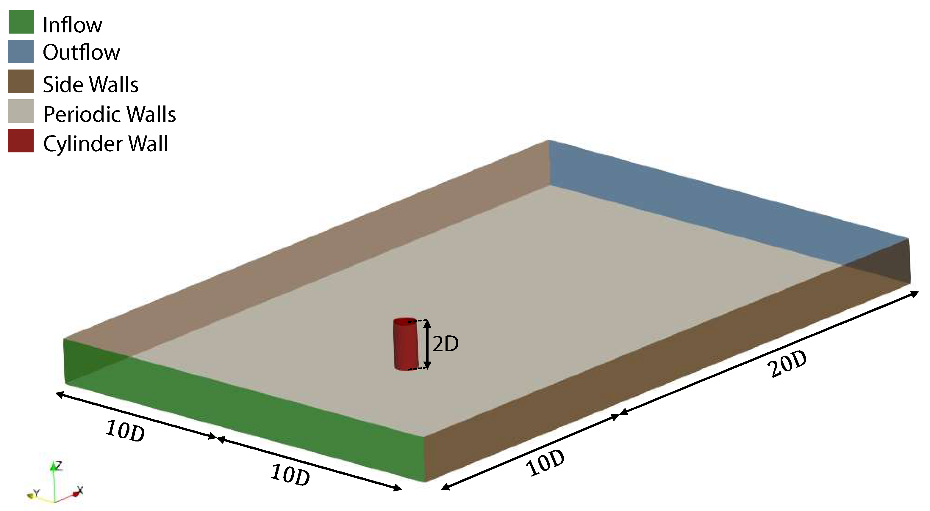
The computational domain was designed following the guidelines established in Saltara et al. [36], who examined a comparable problem for $\mathit{Re}=1\times {10}^4$. As depicted in Figure 1, the circular cylinder of diameter D was positioned $10D$ downstream of the inflow plane and $20D$ upstream of the outflow boundary. Lateral boundaries were symmetrically placed at a distance of $10D$ from the cylinder centerline, ensuring negligible blockage effects.

A critical parameter in three-dimensional simulations of bluff-body wakes is the domain spanwise extent, which must exceed the turbulence correlation length in the spanwise direction to ensure physically consistent vortex dynamics. Importantly, the turbulence correlation length decreases as the Reynolds number increases [1,37]. The present simulations employ a spanwise length of $L/D=2$, following the established practices from both LES and DES studies of high-Reynolds-number circular cylinder flow. Breuer [38] demonstrated via LES at $Re=1.4\times {10}^5$ that increasing the spanwise extent beyond $L/D=2$ does not significantly affect the main wake statistics or force coefficients. Travin et al. [39], employing DES at the same Reynolds number, likewise found that $L/D=2$ captures the essential three-dimensional wake structures. Therefore, the present domain extent is consistent with best practices for accurately representing the physics of interest.

At the inflow, the velocity boundary condition was specified as Dirichlet type, with a uniform value of $U=1$. The desired Reynolds number was imposed by adjusting the kinematic viscosity in the transport properties (the cylinder diameter was $D=1$, so $\mathit{Re}=1/\nu$), a common practice in high-Reynolds-number CFD studies [21,40]. The pressure was prescribed with a Neumann boundary condition (zero normal gradient), while turbulence quantities were imposed as Dirichlet values estimated consistently with the Reynolds number. In particular, the turbulence kinetic energy and specific dissipation rate were scaled according to the turbulence Reynolds number and integral length scale of the flow, as suggested in turbulence modeling guidelines [21,41]. This procedure ensured consistency across the multiple Reynolds regimes investigated, ranging from $5\times {10}^4$ to $1\times {10}^7$, without prescribing arbitrary case-dependent values.

On the lateral boundaries, symmetry plane conditions were applied, enforcing zero normal velocity and zero normal gradients for tangential velocity, pressure, and turbulence quantities. On the spanwise boundaries, cyclic conditions were imposed, effectively replicating an infinitely long, fully submerged cylinder and allowing for periodic continuation of the turbulent structures.

At the cylinder surface, the no-slip condition was enforced for velocity. A Neumann condition (zero gradient) was applied for pressure, while turbulence properties were treated with standard wall functions, consistent with the local $y^{+}$ distribution. This approach has been widely employed in high-Reynolds-number bluff-body simulations, where fully resolving the viscous sublayer is computationally prohibitive [15,40].

At the outflow, the static pressure was fixed at zero, while Neumann conditions (zero normal gradient) were imposed for velocity and turbulence quantities. This combination provided numerical stability while ensuring that the flow exited the domain without artificial reflection of vortical structures.

The drag ($C_D=F_D/\left(\raisebox{1ex}{$1$}\!\left/ \!\raisebox{-1ex}{$2$}\right.\rho U_{\infty }^{2}DL\right)$) and lift ($C_L=F_D/\left(\raisebox{1ex}{$1$}\!\left/ \!\raisebox{-1ex}{$2$}\right.\rho U_{\infty }^{2}DL\right)$) coefficients reported in this work are obtained by full three-dimensional surface integration of the pressure and viscous forces acting on the entire cylindrical surface, as computed by the forceCoeffs utility of OpenFOAM. The integrated forces are projected onto the prescribed streamwise (drag) and transverse (lift) directions and normalized using the reference velocity $U_{\infty }$, reference length D, and the projected reference area $A_{\mathrm{ref}}$, according to the standard definition of force coefficients for incompressible flows.

3.2. Mesh Generation and Refinement

The computational domain was discretized as a non-uniform structured grid, developed based on two-dimensional investigations of the cylinder wake reported by Saltara et al. [36] and extended to the present three-dimensional high-Reynolds-number configurations. The final grid comprised approximately $4.66\times {10}^6$ finite volume cells, with enhanced resolution in the near-wall and wake regions to capture the boundary-layer development and vortex shedding processes accurately.

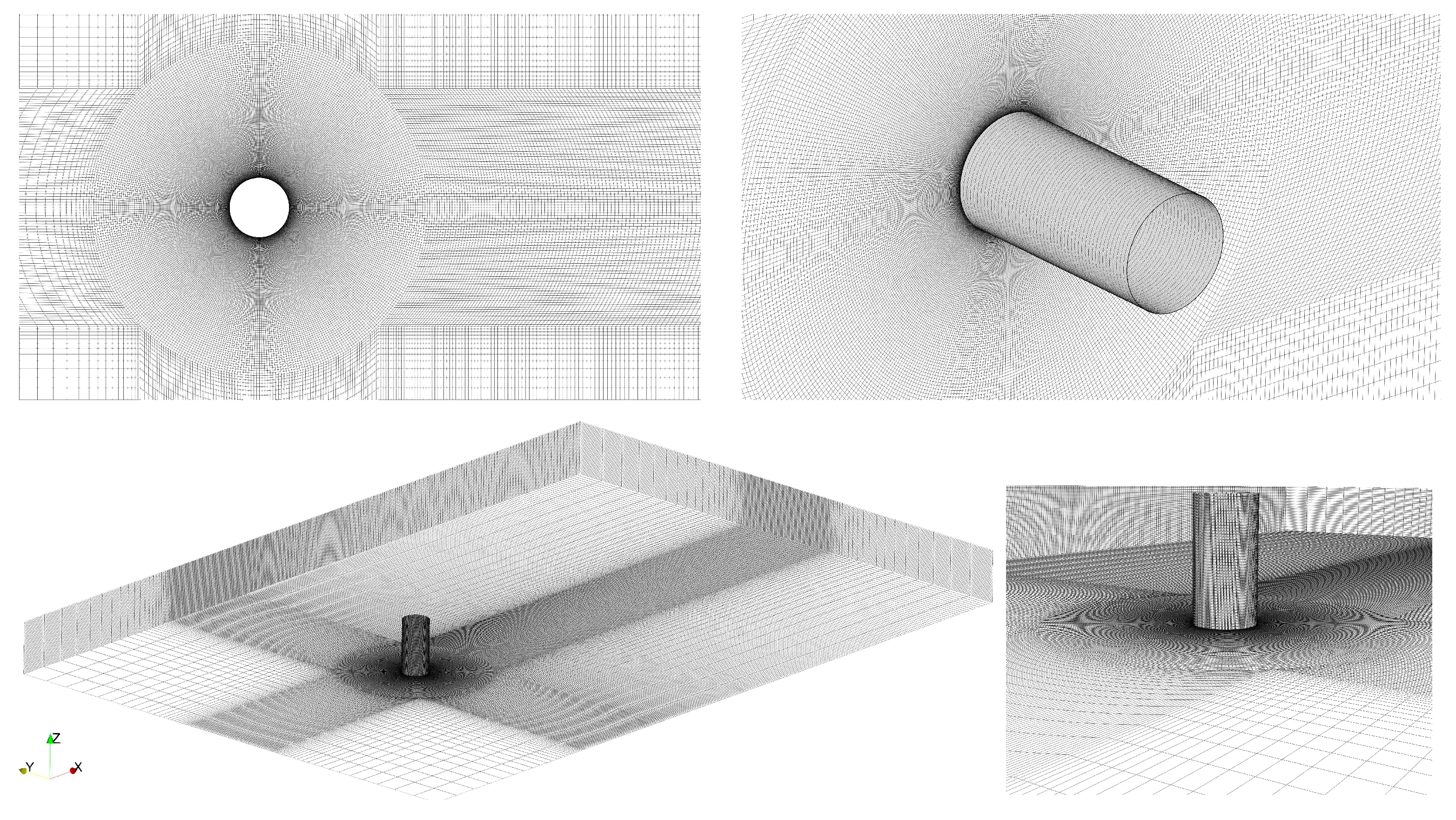
In the wall-normal direction, the first cell height was set to ${10}^{-4}D$. For the Reynolds numbers investigated, this yielded dimensionless wall coordinates of approximately $y^{+}\approx 0.3$, $0.6$, $2.5$, 5, 15, and 40 for $Re=5\times {10}^4$, $1\times {10}^5$, $5\times {10}^5$, $1\times {10}^6$, $3.6\times {10}^6$, and $1\times {10}^7$, respectively. This range of resolutions ensured that, while the lowest Reynolds number cases resolved the viscous sublayer, the most demanding case at $Re={10}^7$ placed the first cell within the logarithmic region, consistent with wall-function requirements widely used in high-Reynolds-number simulations [15,40]. In the spanwise direction, the domain was discretized into 48 divisions, following the guidelines of Catalano et al. [12], who demonstrated the necessity of sufficient spanwise resolution for capturing three-dimensional instabilities at high Reynolds numbers. A representative view of the grid is provided in Figure 2.

The mesh refinement strategy was specifically tailored to the turbulence model, with increased resolution in the shear layers and the near wake, where large-scale, unsteady structures dominate. A coarser mesh was employed in regions far from the cylinder to save computational effort. Similar refinement approaches have been reported in other studies of high-Reynolds-number bluff-body aerodynamics [41,42]. The quality metrics of the mesh satisfied established best-practice guidelines, with a maximum aspect ratio of 83 and a maximum skewness of 0.43, values well within the recommended thresholds for ensuring numerical stability and accuracy [41].

To ensure robust and accurate near-wall treatment across a wide range of $y^{+}$ values, the present study employs the y+lam wall function in OpenFOAM, which adaptively applies the appropriate velocity law depending on the local $y^{+}$: linear (viscous sublayer) law for $y^{+}<5$, logarithmic law for $y^{+}>30$, and a smooth blend for intermediate values [23,32]. This adaptive wall-function methodology has proven reliable and robust in previous hybrid RANS–LES simulations of bluff-body flows and is recommended for engineering applications spanning subcritical to postcritical regimes [31,43].

3.3. Simulations Parameters

In the present simulations, a pressure-based iterative solver employing the Pressure Implicit with Splitting of Operators (PISO) algorithm was adopted to integrate the governing equations in time. The PISO method, originally proposed by Issa [44], is widely recognized for its accuracy and robustness in transient incompressible flows, particularly when strong pressure–velocity coupling is required. In each time step, five sub-iterations and two pressure corrections were applied, following established guidelines for ensuring stability and convergence in high-Reynolds-number simulations [27,45].

The solver implementation was complemented with an additional face-flux correction for pressure, which has been shown to enhance numerical stability during the convergence process, particularly in unsteady flow problems with complex vortex dynamics [33]. A Courant–Friedrichs–Lewy (CFL) number equal to unity was employed for all Reynolds numbers investigated, namely $\mathit{Re}=5\times {10}^4$, $1\times {10}^5$, $5\times {10}^5$, $1\times {10}^6$, $3.6\times {10}^6$, and $1\times {10}^7$. This setting corresponds to the maximum allowed CFL value, meaning that the instantaneous CFL number during the simulations remained below one. The condition corresponds to a non-dimensional time step defined as $\Delta t^{*}=U\Delta t/D$, which yielded $\Delta t^{*}=0.0025$ across all cases. Each simulation was advanced for $80,000$ time steps, ensuring sufficient temporal resolution to capture vortex shedding phenomena and to provide statistically converged flow quantities.

By considering the Strouhal frequencies obtained in each case (see

Table 1. Comparison of mean drag coefficient ($C_{D_{Mean}}$), root mean square of the lift coefficient ($C_{L_{RMS}}$), and Strouhal number ($St$) for all cases investigated in this work, as well as for the previous results reported by de Oliveira et al. [19].

Reynolds Range	CFL	${\mathit{C}}_{{\mathit{D}}_{\mathit{Mean}}}$	${\mathit{C}}_{{\mathit{L}}_{\mathit{RMS}}}$	St
$\mathit{Re}=5\times {10}^4$	1	1.683	0.9718	0.18
$\mathit{Re}=1\times {10}^5$	1	1.102	0.9227	0.18
$\mathit{Re}=5\times {10}^5$	1	0.3502	0.2129	0.21
$\mathit{Re}=1\times {10}^6$ [19]	1	0.5617	0.0498	0.30
$\mathit{Re}=3.6\times {10}^6$ [19]	1	0.4572	0.0645	0.28
$\mathit{Re}=1\times {10}^7$ [19]	1	0.4471	0.0786	0.33

), the chosen temporal resolution corresponded to approximately 1200 time steps per vortex-shedding cycle. Over the entire simulation window, this resulted in about 65 shedding periods being resolved for each Reynolds number investigated.

3.4. Hardware and Parallelization

The simulations were executed on the NEXTGenIO supercomputer at EPCC, University of Edinburgh. For each case, the computational grid was decomposed into 48 sub-domains using the Scotch graph-partitioning algorithm, which provides efficient load balancing and minimizes inter-processor communication in parallel CFD applications. The computations were performed on a single node equipped with two Intel Xeon Platinum 8260M Cascade Lake processors operating at 2.4 GHz, providing 48 physical cores in total, and supported by 192 GB of RAM. For the highest Reynolds number case ($Re=1\times {10}^7$), each 0.1 s of physical simulation required approximately 551 s of wall-clock computational time, leading to a total of roughly 153 h (7344 CPU-hours) for 100 s of simulated flow. In contrast, for the lowest Reynolds number ($Re=5\times {10}^4$), the same interval required about 107 s per 0.1 simulated seconds, totaling 30 h (1440 CPU-hours) for 100 s.

4. Results and Discussion

This section presents a comparative analysis of the flow past a circular cylinder for Reynolds numbers ranging from $5\times {10}^4$ to $1\times {10}^7$, covering subcritical, critical, supercritical, and postcritical regimes. The present study provides new high-fidelity results for the low and intermediate regimes ($Re=5\times {10}^4$, $1\times {10}^5$, $5\times {10}^5$), and integrates them with previous high-Reynolds DES investigations ($Re=1\times {10}^6$, $3.6\times {10}^6$, $1\times {10}^7$) reported in de Oliveira et al. [19]. The intent of this paper is to integrate new and previously published results into a unified, comprehensive discussion, thereby covering all major transition regimes of flow past a circular cylinder. Additionally, the results are benchmarked against established numerical and experimental data from Stringer et al. [46], Catalano et al. [12], and others, to provide a comprehensive understanding of the physical trends observed across regimes.

4.1. Integral Flow Quantities and Reynolds Regimes Analysis

The primary global flow quantities analyzed in this study include the mean drag coefficient ($C_{D_{Mean}}$), the root mean square of the lift coefficient ($C_{L_{RMS}}$), and the Strouhal number ($St$), all evaluated across a wide range of Reynolds numbers and summarized in Table 1. These results provide a comprehensive picture of how the force characteristics and wake structure evolve as the Reynolds number increases, encompassing subcritical, critical, supercritical, and postcritical flow regimes.

A key observation from Table 1 is the significant reduction in mean drag coefficient as the Reynolds number increases from $5\times {10}^4$ to $1\times {10}^6$. This drop is a hallmark of the drag crisis phenomenon, which is driven by the laminar-to-turbulent transition of the boundary layer and the delay in flow separation along the cylinder surface [20,47]. The calculated values for $C_{D_{Mean}}$ decrease from 1.68 in the subcritical regime to about 0.45 in the postcritical regime at $Re=1\times {10}^7$, which closely agrees with data from experimental and high-fidelity numerical studies [12,46]. This sharp decline in drag coefficient indicates a fundamental change in wake dynamics, as the separated shear layers shift downstream and the recirculation zone becomes narrower [1,20].

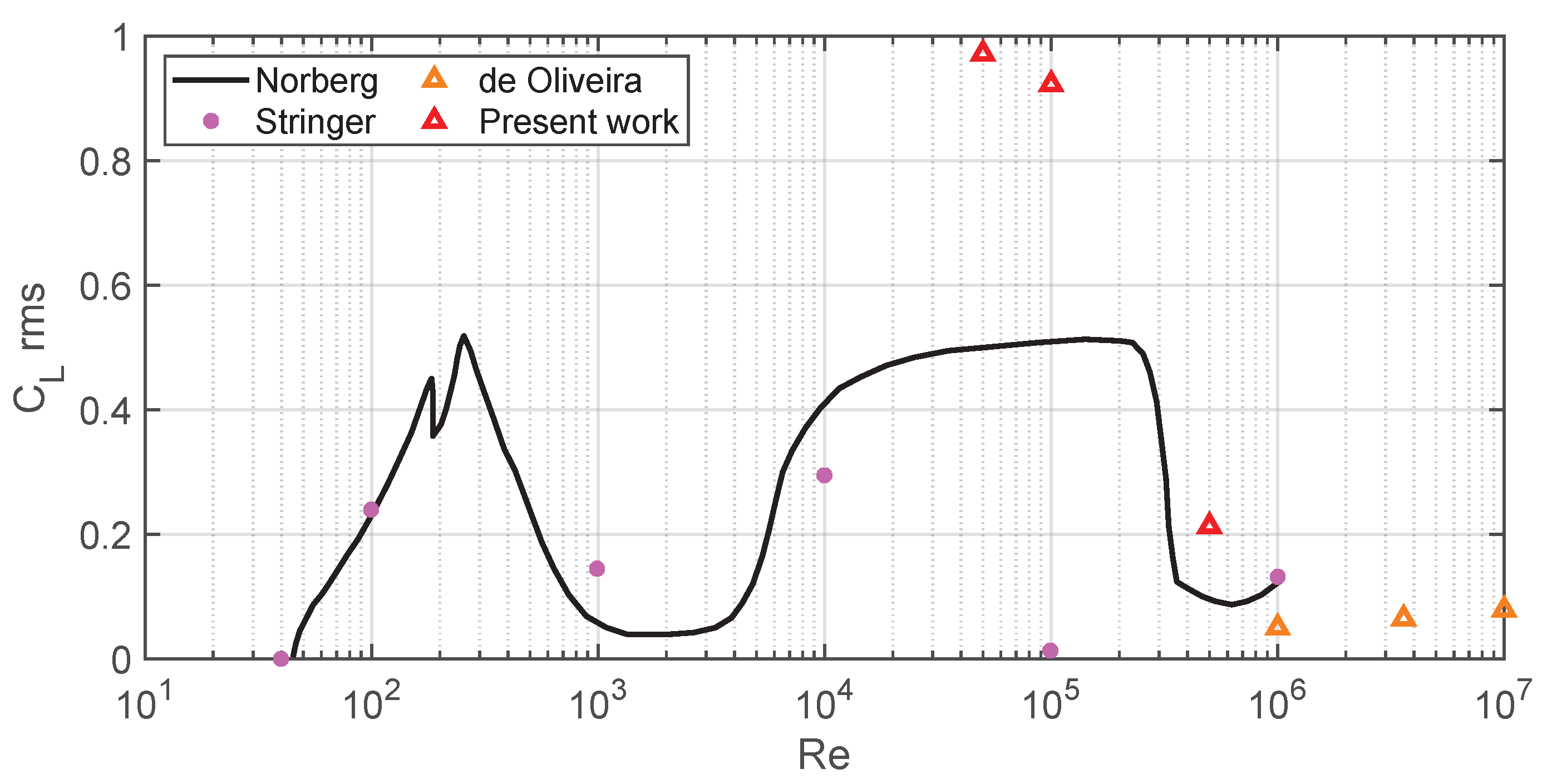
The connection between three-dimensional vortex shedding and hydrodynamic force fluctuations is evident in these trends. As the flow evolves from coherent, spanwise-aligned vortex structures in the subcritical and critical regimes to highly fragmented, three-dimensional wakes at higher Reynolds numbers, the amplitude and regularity of hydrodynamic forces are directly affected. In particular, the loss of spanwise coherence leads to a sharp reduction in the root mean square of the lift coefficient ($C_{L_{RMS}}$), as shown in Figure 3, and a broadening of the spectral content of lift and drag fluctuations. These results are in agreement with the literature [1,12,20] and demonstrate that the observed reduction in force fluctuation intensity is causally linked to the breakdown of organized vortex shedding and the onset of three-dimensional turbulence in the wake.

The fluctuations in lift force, represented by $C_{L_{RMS}}$, also show a marked dependence on Reynolds number. As shown in Table 1, the lift coefficient fluctuations are large and highly regular at lower Reynolds numbers, which is a result of strong, two-dimensional vortex shedding that dominates the subcritical regime. With increasing Reynolds number, particularly into the critical and supercritical regimes, the magnitude of these fluctuations drops sharply. This reduction points to a transition towards a more three-dimensional and turbulent wake, where the coherence of vortex structures is diminished [1,46].

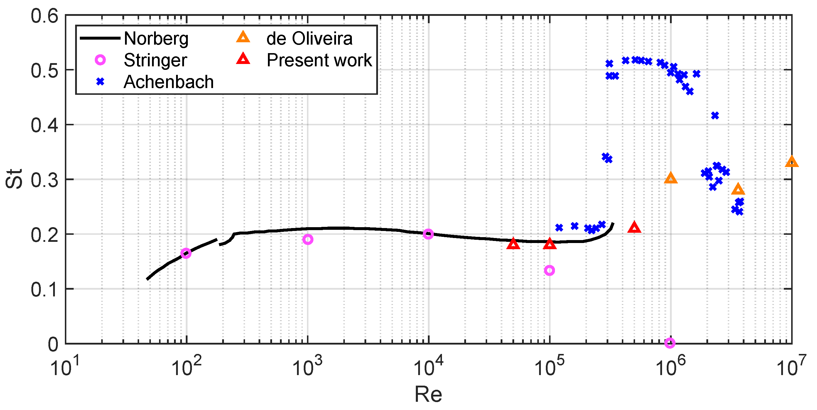
Additionally, the Strouhal number, which describes the normalized vortex shedding frequency, remains nearly constant at around 0.18 for lower Reynolds numbers. As the flow transitions into the supercritical and postcritical regimes, the Strouhal number increases to values near 0.3 and above. This behavior corresponds to the narrowing of the wake and the increase in vortex shedding frequency as the boundary layer becomes turbulent and flow separation is further delayed. These results are in agreement with the experimental data from Achenbach [47] and Norberg [48], and modern high-fidelity simulations from [12,46], which can also be observed in Figure 4.

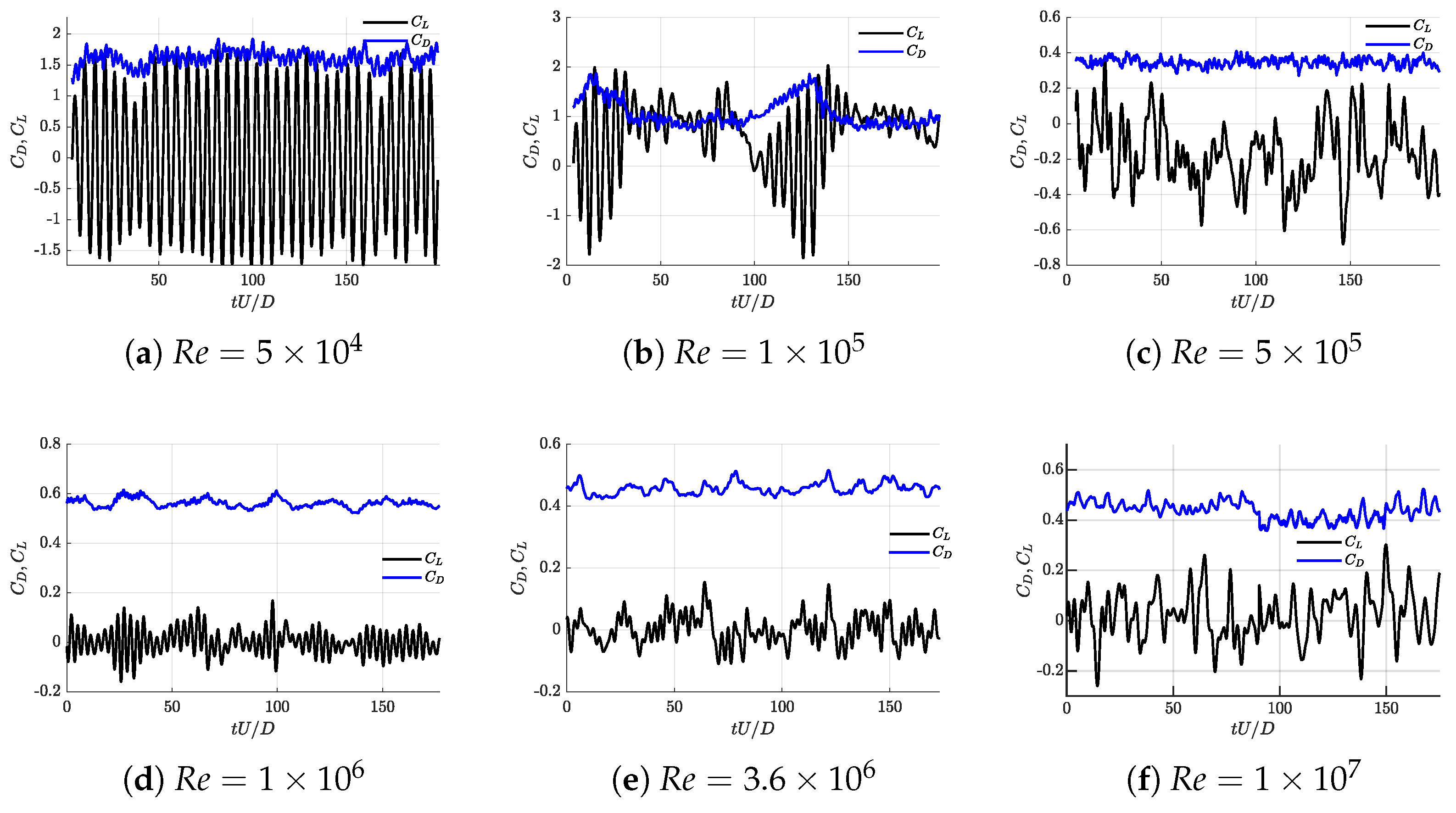
The time series of $C_L$ and $C_D$ shown in Figure 5 provide a clear illustration of these transitions. At low Reynolds numbers, both signals display strong periodicity and high amplitude, reflecting the dominance of organized two-dimensional vortex shedding [1]. This behavior has important consequences for flow-induced vibrations and structural fatigue in practical engineering systems. As the Reynolds number increases, particularly above $1\times {10}^6$, the force signals become less periodic, and the amplitude of fluctuations decreases, which is consistent with the onset of more chaotic, three-dimensional wake dynamics. These findings are in agreement with both experimental data and theoretical models described in the literature [20].

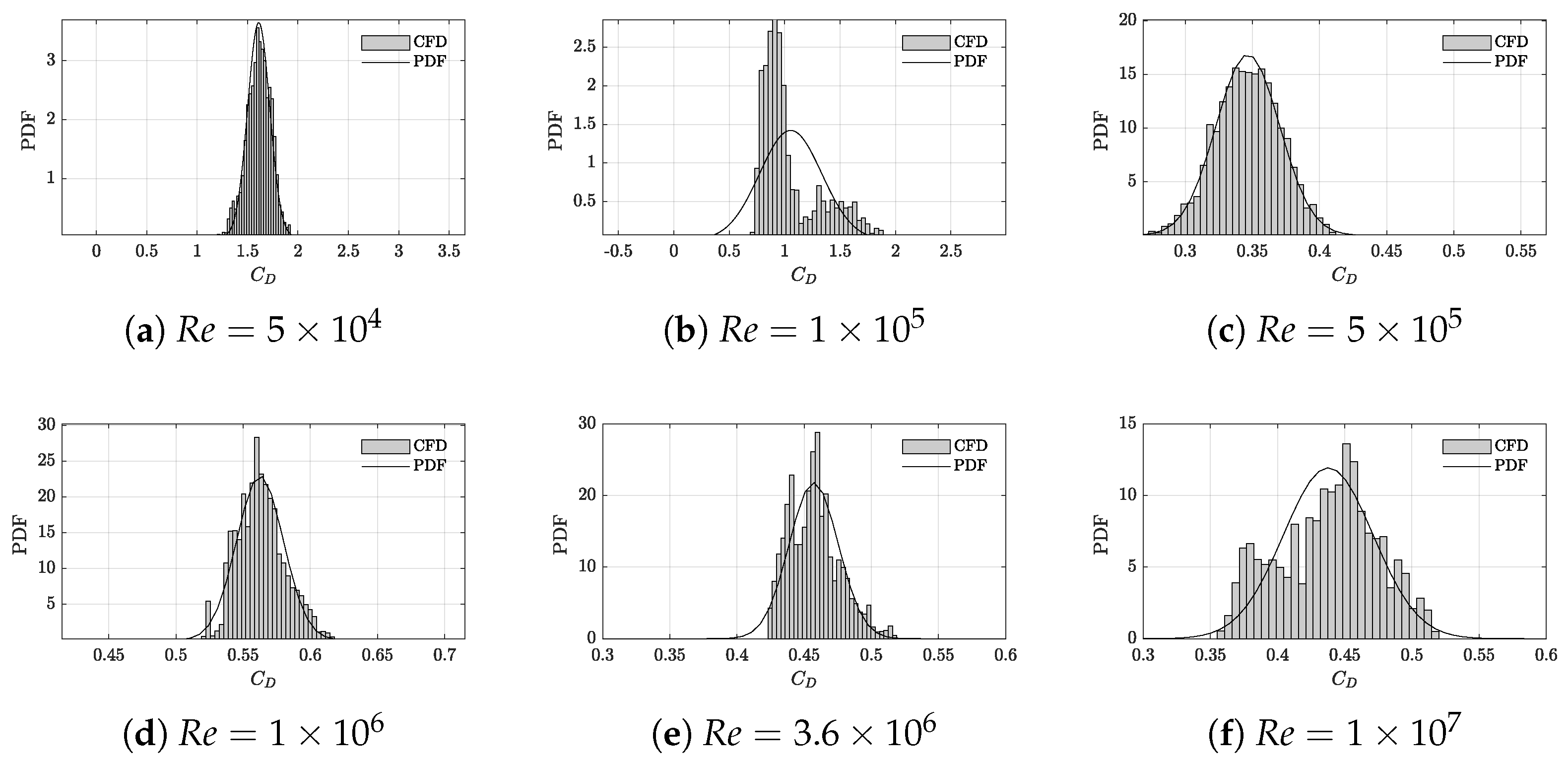
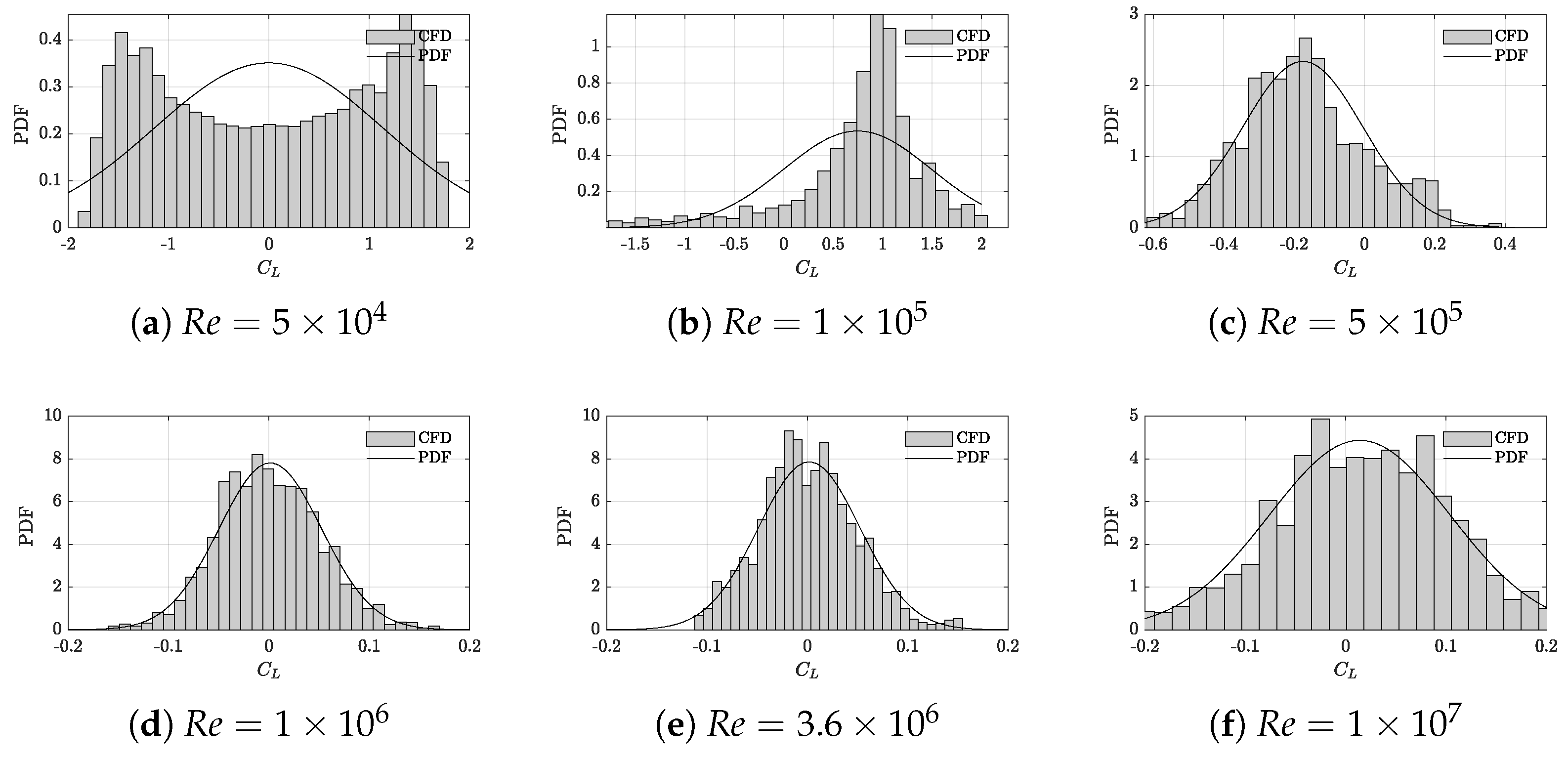
To further quantify the statistical nature of the unsteady hydrodynamic loads observed in the time series, the probability density functions (PDFs) of the drag and lift coefficients were computed from the fully time-resolved CFD signals for all Reynolds numbers investigated. The probability density functions (PDFs) of the lift and drag coefficients shown in Figure 6 and Figure 7, respectively, provide a detailed statistical description of the unsteady loading acting on the cylinder across the investigated Reynolds number range. The PDF represents the normalized frequency of occurrence of a given force coefficient value, thus quantifying not only the mean behavior but also the variability, intermittency, and symmetry of the force fluctuations. At low Reynolds numbers ($Re=5\times {10}^4$ and $Re=1\times {10}^5$), both $C_D$ and $C_L$ PDFs exhibit broader and bimodal distributions, reflecting the strong periodic vortex shedding and the high level of coherence of the wake observed in the corresponding time series. As the Reynolds number increases into the critical regime ($Re=5\times {10}^5$), the distributions progressively narrow and approach a near-Gaussian shape, indicating a reduction in the regularity of vortex shedding and the onset of enhanced three-dimensional instabilities in the wake. In the supercritical, transcritical, and postcritical regimes ($Re\ge {10}^6$), the PDFs of both $C_D$ and $C_L$ become sharply peaked and closely Gaussian, demonstrating that the force fluctuations are increasingly governed by fully developed turbulent dynamics rather than by organized periodic structures. This statistical transition is fully consistent with the marked reduction in $C_{L,\mathrm{RMS}}$, the stabilization of the mean drag coefficient following the drag crisis, and the loss of spanwise coherence observed in the wake visualizations (Figure 3 and Figure 4). Together, the PDFs of $C_D$ and $C_L$ provide a complementary quantitative confirmation of the progressive breakdown of coherent vortex shedding and the dominance of three-dimensional turbulent wake dynamics at high Reynolds numbers.

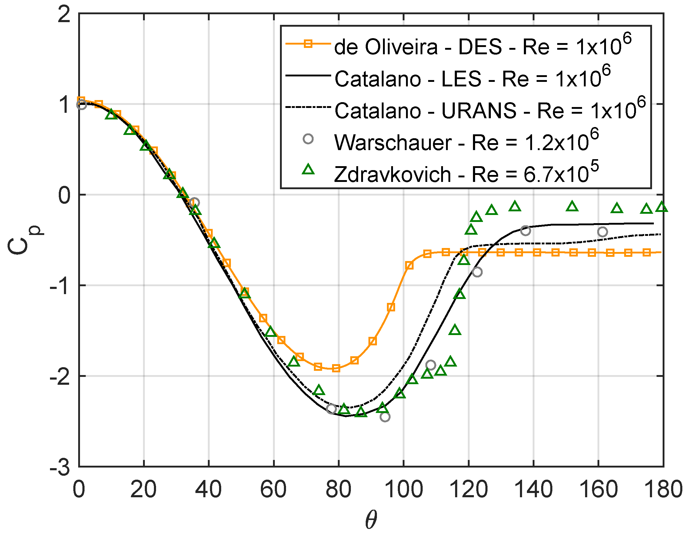
As the force signals evolve across Reynolds regimes, these trends are closely linked to changes in surface pressure distribution and wake separation around the cylinder. Analyzing the time-averaged pressure coefficient provides deeper insight into the underlying physics responsible for the observed variations in drag and lift coefficients. A detailed comparison of the time-averaged pressure coefficient ($C_p=p/\left(\raisebox{1ex}{$1$}\!\left/ \!\raisebox{-1ex}{$2$}\right.\rho U_{\infty }^2\right)$) over the cylinder surface at $Re=1\times {10}^6$ is shown in Figure 8. Here, results from the DES calculations from our previous work [19] are contrasted with LES and URANS data from Catalano et al. [12], as well as experimental measurements from Warschauer ($Re=1.2\times {10}^6$) and Falchsbart in Zdravkovich ($Re=6.7\times {10}^5$) [20,49].

The present DES results reproduce the main trends of the pressure coefficient, including the delayed separation and reduction in base pressure that characterize the onset of the drag crisis. Agreement with high-fidelity LES and experimental data is observed in the attached boundary layer region and along most of the cylinder surface. However, some discrepancies become apparent near the separation point and in the wake, where the DES values tend to deviate from the reference curves.

These discrepancies can be attributed in part to the inherent characteristics of the Detached Eddy Simulation methodology. DES models are known to blend RANS and LES formulations depending on the local grid and flow features, which may lead to a less precise prediction of the separation location and the fine-scale wake dynamics, especially when compared to full wall-resolved LES or highly resolved experiments [12].

Additionally, the accurate capture of pressure recovery and the subtle three-dimensional effects in the supercritical regime is highly sensitive to grid resolution, turbulence modeling, and numerical implementation [12,20]. The DES approach captures the main characteristics of the pressure distribution, including the key features associated with the drag crisis at high Reynolds numbers. The differences observed in the base pressure region suggest that alternative strategies for mesh refinement or enhancements in turbulence modeling may improve the prediction of separation and wake behavior, particularly in transitional flow regimes.

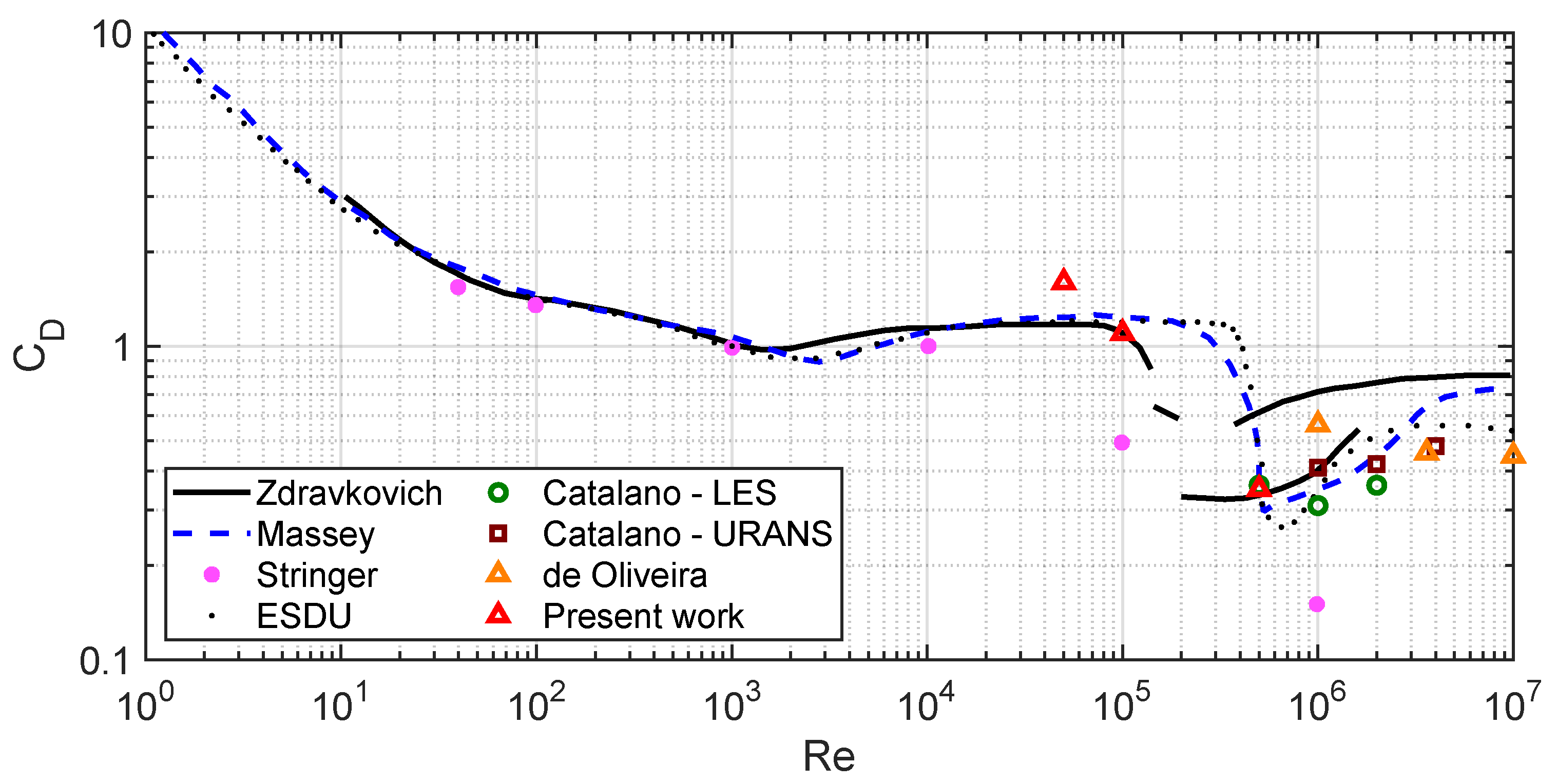
The variation in the mean drag coefficient ($C_{D_{Mean}}$) as a function of the Reynolds number is a fundamental feature for analyzing the flow around bluff bodies and has been extensively studied both experimentally and numerically. As shown in Figure 9, the results from the present study are in agreement with the classic trend reported in the literature [1,20,47]. At low Reynolds numbers, $C_{D_{Mean}}$ decreases gradually as the boundary layer remains laminar and separates early, leading to a broad wake. As $Re$ approaches the critical regime, the curve exhibits a pronounced drop, commonly referred to as the drag crisis. This behavior is attributed to the transition of the boundary layer from laminar to turbulent before separation, causing delayed separation, a narrower wake, and consequently, a sharp reduction in drag [4,42]. For $Re>{10}^6$, the drag coefficient stabilizes at lower values as the flow fully transitions into the supercritical and postcritical regimes, where the wake becomes increasingly turbulent and three-dimensional. The results from the present study, as well as from DES, LES, and URANS simulations by de Oliveira et al. [19], Catalano et al. [12], and Stringer et al. [46], are consistent with the experimental data compiled by Zdravkovich [4], Massey [50], and the ESDU database [51]. Minor discrepancies across the datasets can be attributed to differences in experimental setups, numerical methodologies, and the sensitivity of drag to surface roughness and boundary layer tripping, which are widely recognized challenges in representing flows governed by high Reynolds numbers [1,47].

The root mean square of the lift coefficient ($C_{L_{RMS}}$) provides a measure of the intensity of unsteady transverse forces acting on the cylinder due to vortex shedding. Figure 3 demonstrates how $C_{L_{RMS}}$ varies with Reynolds number, highlighting the transitions between distinct wake regimes. At low $Re$, $C_{L_{RMS}}$ rises sharply as periodic vortex shedding becomes well established, reaching peak values in the subcritical and lower critical regimes. This is in agreement with experimental observations by Norberg [48], and with the simulations of Stringer et al. [46] and de Oliveira et al. [19]. As $Re$ increases further and the flow transitions into the supercritical and postcritical regimes, $C_{L_{RMS}}$ drops significantly. This decrease is attributed to the increasing three-dimensionality and turbulence of the wake, which disrupt the coherence of vortex structures and reduce the amplitude of lift fluctuations [1,20]. The agreement among the present numerical results and the referenced experimental and computational studies supports the conclusion that both the methodology and grid resolution employed are adequate to capture the primary trends in unsteady lift behavior across regimes. Remaining differences can often be traced to the sensitivity of lift fluctuations to spanwise correlation length, surface roughness, and even the specific implementation of turbulence models [46,48].

As illustrated in Figure 4, regarding the Strouhal number, the results from the present study are in close agreement with both experimental and numerical benchmarks across a wide range of Reynolds numbers. For subcritical and early critical regimes, $St$ remains nearly constant, reflecting a stable vortex shedding process dominated by periodic, mostly two-dimensional structures. This behavior transitions as the Reynolds number increases, with $St$ rising sharply in the supercritical and postcritical regimes due to the delayed separation and the narrowing of the wake, which are directly linked to the drag crisis and the reduction in mean drag coefficient previously discussed. The agreement with data from Norberg [48], Achenbach [47], Stringer et al. [46], and de Oliveira et al. [19] further supports the robustness of the present numerical approach in capturing the coupled evolution of unsteady vortex dynamics and hydrodynamic loading. The observed trends underscore the importance of accurately predicting Strouhal number variations for offshore structures, as changes in vortex shedding frequency can lead to resonance and flow-induced vibrations, thereby impacting both structural integrity and operational performance.

4.2. Quantitative Validation and Error Analysis

While the evolution of mean drag, lift, and Strouhal number demonstrates trends consistent with the literature, it is essential to quantify the accuracy and reliability of the DES results through direct, quantitative comparison with established experimental and numerical data.

Table 2. Quantitative comparison of mean drag coefficient ($C_{D_{Mean}}$) between the present DES results and selected reference datasets.

Reynolds Number	${\mathit{C}}_{\mathit{D},\mathit{DES}}$ (Present)	${\mathit{C}}_{\mathit{D},\mathit{Ref}}$ (Literature)	Error (%)
$5\times {10}^4$	1.683	1.63 [1]	3.2
$1\times {10}^5$	1.102	1.12 [1]	1.6
$5\times {10}^5$	0.3502	0.34 [2]	3.0
$1\times {10}^6$	0.5617	0.54 [2]	4.0
$3.6\times {10}^6$	0.4572	0.44 [2]	3.9
$1\times {10}^7$	0.4471	0.43 [2]	4.0

^[1] Experimental values from Zdravkovich [4]; ^[2] Experimental values from Achenbach [47] and Massey [50].

summarizes the percentage error of the mean drag coefficient ($C_{D_{Mean}}$) predicted in this work relative to widely cited references for selected Reynolds numbers. The percentage error is calculated as $\mathrm{Error}=100 \times |C_{D,DES}-C_{D,Ref}|/C_{D,Ref}$.

As seen in Table 2, the percentage errors in $C_{D_{Mean}}$ are generally below 5% for all Reynolds numbers investigated, indicating that the DES methodology yields results in close quantitative agreement with benchmark experiments and previous high-fidelity simulations. The largest deviations are observed at the highest Reynolds numbers, where the sensitivity to turbulence modeling, mesh resolution, and near-wall treatment is most pronounced. Notably, the present DES approach slightly overpredicts the mean drag coefficient in the postcritical regime, consistent with known tendencies of hybrid RANS–LES methods when compared with full wall-resolved LES or experiments on smooth cylinders.

Despite these sources of uncertainty, the quantitative agreement (within 5%) for the mean drag coefficient is within the range commonly reported for DES and hybrid RANS–LES approaches in bluff body flows at high Reynolds numbers [12,16,46]. This level of accuracy is sufficient for most engineering applications, especially for preliminary design and the assessment of flow-induced loads on offshore structures.

Furthermore, the trends observed for the Strouhal number and the root-mean-square lift coefficient also fall within the experimental scatter reported in the literature, reinforcing the overall reliability of the present simulations. For future work, additional grid sensitivity studies, inclusion of surface roughness effects, and the use of inflow turbulence generation could further reduce these discrepancies.

4.3. Flow Structures

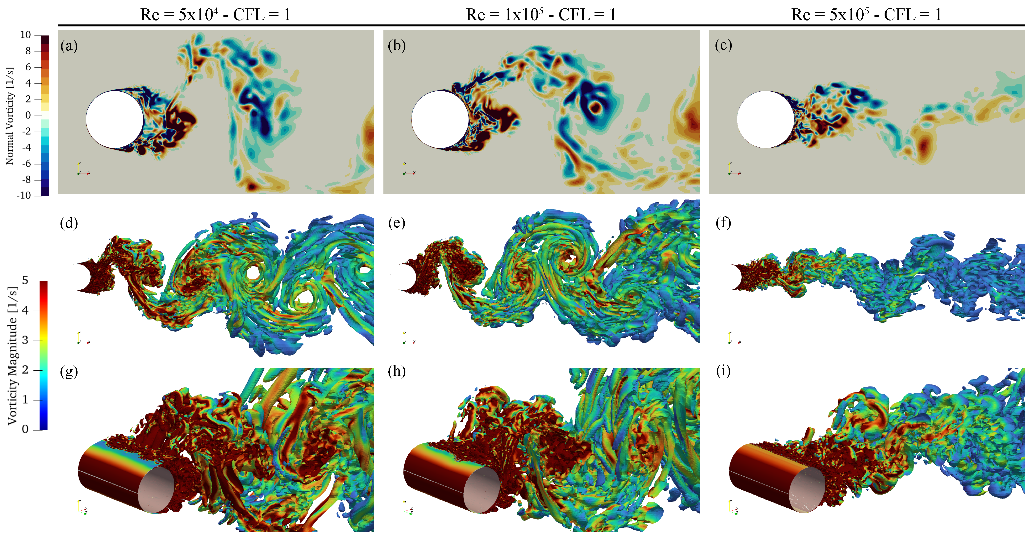
The instantaneous flow visualizations presented in Figure 10 provide direct insight into the wake dynamics and vortex formation mechanisms for the subcritical and critical Reynolds number regimes investigated in this work. At $Re=5\times {10}^4$ and $Re=1\times {10}^5$, the wake is characterized by the formation of large, coherent two-dimensional vortices that are periodically shed from the cylinder surface. The vorticity fields and Q-criterion isosurfaces reveal the classic von Kármán vortex street, where the alternating shedding of vortices dominates the wake structure and induces strong periodic lift and drag fluctuations, as previously discussed. This flow organization is consistent with canonical visualizations and laboratory observations reported by Zdravkovich [20], Williamson [1], and Bearman [34], and is reflected in the elevated $C_{L_{RMS}}$ and nearly constant Strouhal number observed for this regime. As the Reynolds number increases to $Re=5\times {10}^5$, subtle but significant changes in the wake structure become apparent. While large-scale vortex shedding persists, there is increased evidence of three-dimensional instabilities and fragmentation in the wake, particularly downstream of the cylinder. The Q-criterion visualizations show the development of smaller-scale structures and a reduction in spanwise coherence, indicating the initial stages of transition towards the critical regime. This evolution in wake dynamics is aligned with that fact that the flow becomes increasingly three-dimensional and turbulent [1,20,42].

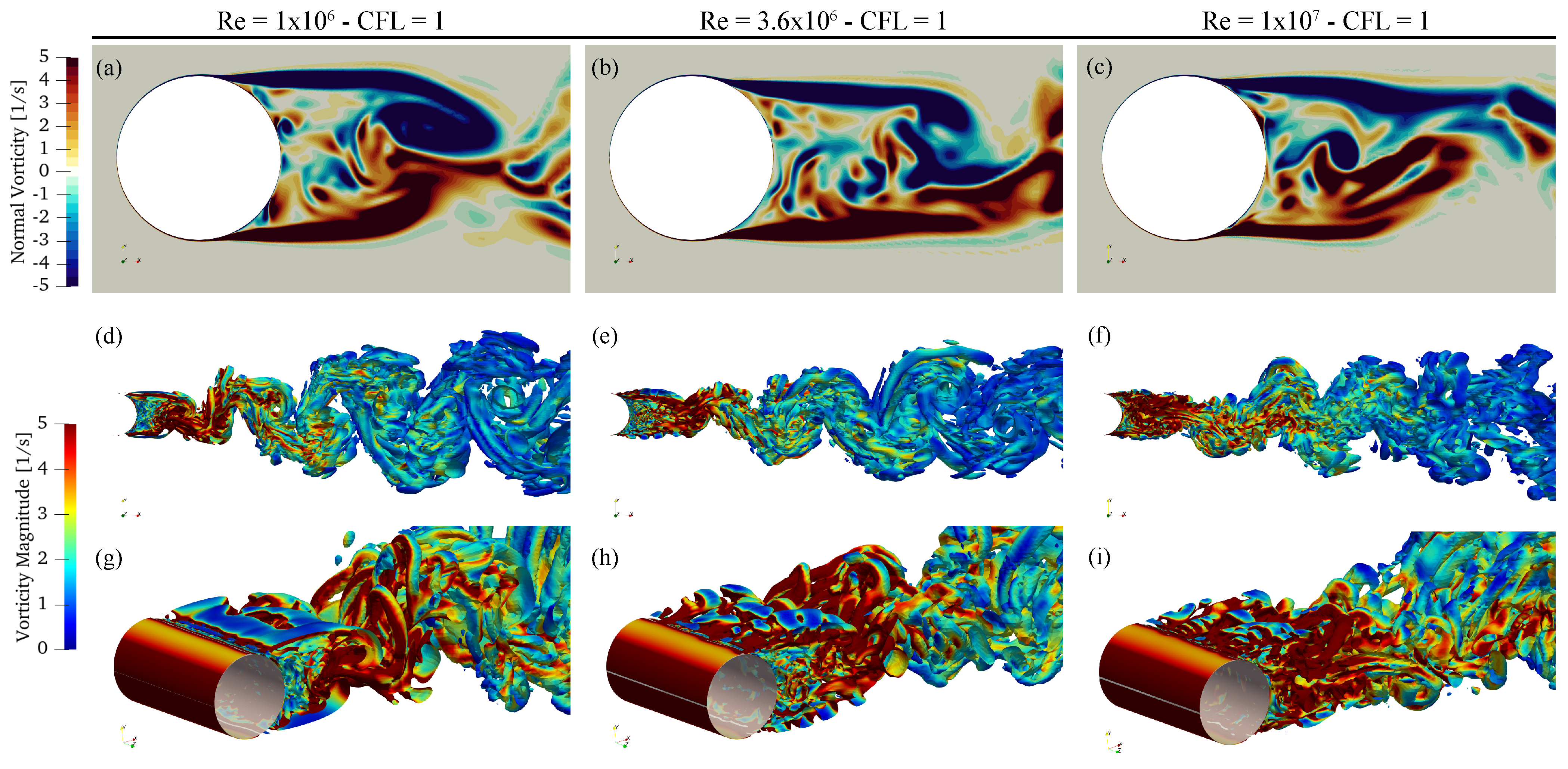
Transitioning to higher Reynolds numbers, as shown in Figure 11 for the cases previously reported by de Oliveira et al. [19], the wake structure changes dramatically. For $Re=1\times {10}^6$ and above, the vorticity fields and Q-criterion isosurfaces indicate a highly fragmented and disordered wake, dominated by fine-scale turbulent structures and the loss of periodic vortex shedding. The flow separation is significantly delayed, and the recirculation zone narrows, consistent with the classic signatures of the drag crisis. These features have been well documented in experimental studies by Achenbach [47] and Roshko [52], and in high-fidelity numerical investigations [12,46]. The suppression of organized vortex shedding and the dominance of turbulence in the wake result in a substantial reduction in drag and a sharp change in the Strouhal number, as observed in the previous section.

The comparison across Figure 10 and Figure 11 for the different regimes demonstrates a clear progression from organized, two-dimensional vortex dynamics at low Reynolds numbers to highly three-dimensional and turbulent wake behavior in the supercritical and postcritical regimes. This transition is central to understanding the fluid–structure interaction phenomena relevant for offshore engineering, as the nature of wake dynamics directly impacts flow-induced vibrations, structural fatigue, and operational stability of cylindrical structures exposed to ocean currents and waves.

5. Concluding Remarks

This study presented high-fidelity detached eddy simulations (DES) of the flow around an infinitely long smooth circular cylinder, systematically covering the subcritical, critical, supercritical, and postcritical Reynolds regimes ($5\times {10}^4$ to $1\times {10}^7$). The numerical methodology, based on OpenFOAM with Menter’s k-$\omega$ SST turbulence model and careful near-wall resolution, enabled accurate investigation of the evolution of wake structures, force coefficients, and unsteady flow phenomena across this broad range.

The results corroborate the classical hallmarks of transitional flow regimes as established by Zdravkovich [20], Achenbach [47], Roshko [52], and Williamson [1]. Key observations include the sharp drop in mean drag coefficient (the drag crisis), the progressive delay of boundary layer separation, and the significant changes in Strouhal number and lift fluctuations as the Reynolds number increases. These features were clearly captured by the present DES methodology and validated against benchmark experimental and numerical datasets [12,20,46,48,50].

A unified analysis of mean drag, root mean square lift, and Strouhal number confirms that the present simulations reproduce the expected trends: a marked reduction in drag coefficient and lift fluctuations with increasing $Re$, and a rise in Strouhal number in the supercritical regime. The evolution of the wake, from organized two-dimensional vortex streets at low $Re$ to highly fragmented and turbulent wakes at high $Re$, is consistent with canonical visualizations and the theoretical framework for bluff-body flows [1,20].

The DES approach demonstrated strong robustness across all regimes, but some limitations remain. In particular, discrepancies observed in the prediction of base pressure and separation location highlight the need for further mesh refinement or hybrid modeling strategies, especially in the transitional and supercritical regimes. These observations echo the findings of Catalano et al. [12] and Stringer et al. [46]. Further investigation into the sensitivity of DES and hybrid URANS–LES approaches to grid resolution, wall functions, and inflow turbulence conditions would provide valuable guidance for future simulations of large-scale offshore structures.

From a quantitative standpoint, the DES results show mean drag coefficients that are generally within 5% of experimental benchmarks across all regimes, demonstrating the robustness and reliability of the adopted methodology (see Section 4.2). The main numerical uncertainties stem from the interplay among mesh resolution, wall treatment, and subgrid modeling, especially in transitional and supercritical regimes, where small changes in grid density can affect separation location and base pressure predictions. The scarcity of experimental data against which the results of our calculations could be validated is an important limitation of this work.

Future investigations should focus on systematic mesh and domain refinement, uncertainty quantification using alternative indices (e.g., LES-IQ, ER-QI), and the incorporation of realistic inflow turbulence and surface roughness effects. Expanding the scope to include fluid–structure interaction and flexible cylinder response will be particularly relevant for offshore engineering applications, such as risers, cables, and support structures exposed to vortex-induced vibrations. The continuous development of open-source CFD platforms and high-performance computing resources is expected to further advance the predictive capability and engineering relevance of simulations in high-Reynolds-number flows.

The overall research provides a comprehensive investigation of unsteady wake dynamics and force coefficients for circular cylinders across subcritical, critical, and transitional Reynolds number regimes. By integrating new results with previous studies, the analysis offers a more unified and detailed understanding of flow physics throughout these regimes. The use of a robust computational methodology, implemented in open-source software, demonstrates both the reliability and accessibility of high-fidelity simulations for practical analysis. The findings establish a valuable numerical benchmark and deliver relevant insights for the design and assessment of offshore structures exposed to vortex-induced forces. Continued advances in turbulence modeling, mesh refinement strategies, and fluid–structure interaction simulations are expected to further enhance the predictive capability of computational fluid dynamics for complex, high-Reynolds-number flows.

References

1. Williamson, C.H.K. Vortex dynamics in the cylinder wake. Annu. Rev. Fluid Mech. 1996, 28, 477–539. [Google Scholar] [CrossRef]
2. Bearman, P.W.; Obasaju, E.D. The interaction between a bluff body and a downstream flat plate in a uniform flow. J. Fluid Mech. 1969, 35, 431–448. [Google Scholar]
3. Achenbach, E. Influence of surface roughness on the cross flow around a circular cylinder. J. Fluid Mech. 1971, 46, 321–335. [Google Scholar] [CrossRef]
4. Zdravkovich, M.M. Conceptual Aspects of Bluff Body Aerodynamics; Springer: Berlin/Heidelberg, Germany, 1990. [Google Scholar]
5. Roshko, A. Experiments on the flow past a circular cylinder at very high Reynolds number. J. Fluid Mech. 1961, 10, 345–356. [Google Scholar] [CrossRef]
6. Carlson, D.; Chaplin, J. Vortex induced vibration of large diameter risers and pipelines. Philos. Trans. R. Soc. A 2018, 376, 20170102. [Google Scholar]
7. Blevins, R.D. Flow Induced Vibration; Van Nostrand Reinhold: New York, NY, USA, 1976. [Google Scholar]
8. Achenbach, E. Vortex shedding from cylinders at high Reynolds numbers. J. Fluid Mech. 1981, 109, 239–251. [Google Scholar] [CrossRef]
9. Niemann, H.; Hölscher, N. Review of flow past bluff bodies with applications to circular cylinders. J. Wind Eng. Ind. Aerodyn. 1990, 33, 197–209. [Google Scholar] [CrossRef]
10. Baggett, J.S.; Jiménez, J.; Kravchenko, A.G.; Moin, P. Resolution requirements for large eddy simulation of shear flows. In Annual Research Briefs; Center for Turbulence Research, Stanford Univ.: Stanford, CA, USA, 1997; pp. 51–66. [Google Scholar]
11. Fung, Y.C. Fluctuating lift and drag on a circular cylinder at high Reynolds numbers. J. Appl. Mech. 1960, 27, 336–337. [Google Scholar]
12. Catalano, P.; Wang, M.; Bertoglio, J.P.; Shao, L. Numerical simulation of the flow around a circular cylinder at high Reynolds numbers. Int. J. Heat Fluid Flow 2003, 24, 463–469. [Google Scholar] [CrossRef]
13. Kim, J.; Choi, H. Prediction of flow over a circular cylinder at high Reynolds numbers. Phys. Fluids 2005, 17, 085101. [Google Scholar]
14. Pasam, R.S.; Prucker, T.; Dinkelacker, F.; Worth, N.A. Influence of surface roughness on postcritical flow over circular cylinders revisited. J. Fluid Mech. 2023, 964, A23. [Google Scholar] [CrossRef]
15. Menter, F.R. Two-equation eddy-viscosity turbulence models for engineering applications. AIAA J. 1994, 32, 1598–1605. [Google Scholar] [CrossRef]
16. Traverso, S.; Menter, F.R.; Deng, G. Assessing DES and hybrid RANS–LES approaches for high Reynolds number bluff body flows. J. Fluids Eng. 2020, 142, 061201. [Google Scholar]
17. Spalart, P.R.; Jou, W.H.; Strelets, M.; Allmaras, S.R. Comments on the feasibility of LES for wings, and on a hybrid RANS/LES approach. In Advances in DNS/LES; Liu, C., Liu, Z., Eds.; Greyden Press: Columbus, OH, USA, 1997; pp. 137–147. [Google Scholar]
18. Launder, B.E.; Spalding, D.B. The numerical computation of turbulent flows. Comput. Methods Appl. Mech. Eng. 1974, 3, 269–289. [Google Scholar] [CrossRef]
19. de Oliveira, M.; da Silva, L.S.P.; Saltara, F.; Carmo, B.S.; Gonçalves, R.T. Temporal discretization investigation of the unsteady loading on an infinitely long cylinder in high Reynolds numbers using DES. In Proceedings of the ASME 2023 International Conference on Ocean, Offshore and Arctic Engineering (OMAE2023), Melbourne, VIC, Australia, 11–16 June 2023. Paper OMAE2023-104427. [Google Scholar] [CrossRef]
20. Zdravkovich, M.M. Flow Around Circular Cylinders. Vol. 1: Fundamentals; Oxford University Press: Oxford, UK, 1997. [Google Scholar]
21. Pope, S.B. Turbulent Flows; Cambridge University Press: Cambridge, UK, 2001. [Google Scholar] [CrossRef]
22. Ferziger, J.H.; Perić, M.; Street, R.L. Computational Methods for Fluid Dynamics, 4th ed.; Springer: Cham, Switzerland, 2020. [Google Scholar] [CrossRef]
23. Wilcox, D.C. Turbulence Modeling for CFD, 2nd ed.; DCW Industries: La Cañada, CA, USA, 1998. [Google Scholar]
24. Spalart, P.R. Strategies for turbulence modelling and simulations. Int. J. Heat Fluid Flow 2000, 21, 252–263. [Google Scholar] [CrossRef]
25. Menter, F.R. Zonal two equation kω turbulence models for aerodynamic flows. In Proceedings of the 23rd Fluid Dynamics, Plasmadynamics, and Lasers Conference, Orlando, FL, USA, 6–9 July 1993. AIAA Paper 1993-2906. [Google Scholar] [CrossRef]
26. Spalart, P.R. Detached-eddy simulation. Annu. Rev. Fluid Mech. 2009, 41, 181–202. [Google Scholar] [CrossRef]
27. Versteeg, H.K.; Malalasekera, W. An Introduction to Computational Fluid Dynamics: The Finite Volume Method, 2nd ed.; Pearson: Harlow, UK, 2007. [Google Scholar]
28. Moukalled, F.; Mangani, L.; Darwish, M. The Finite Volume Method in Computational Fluid Dynamics; Springer: Cham, Switzerland, 2016. [Google Scholar] [CrossRef]
29. Weller, H.G.; Tabor, G.; Jasak, H.; Fureby, C. Controlling convection schemes in the finite volume method. Comput. Phys. Commun. 1998, 85, 273–285. [Google Scholar]
30. Jasak, H. Error Analysis and Estimation for the Finite Volume Method with Applications to Fluid Flows. Ph.D. Thesis, Imperial College London, London, UK, 1996. [Google Scholar]
31. de Oliveira, M.; Puraca, R.C.; Carmo, B.S. A study on the influence of the numerical scheme on the accuracy of blade-resolved simulations employed to evaluate the performance of the NREL 5 MW wind turbine rotor in full scale. Energy 2023, 283, 128394. [Google Scholar] [CrossRef]
32. Liu, F. A thorough description of how wall functions are implemented in OpenFOAM. In Proceedings of CFD with OpenSource Software; Chalmers University of Technology: Gothenburg, Sweden, 2016. [Google Scholar]
33. de Oliveira, M.; Puraca, R.C.; Carmo, B.S. Blade-resolved numerical simulations of the NREL offshore 5 MW baseline wind turbine in full scale: A study of proper solver configuration and discretization strategies. Energy 2022, 254, 124368. [Google Scholar] [CrossRef]
34. Bearman, P.W. Vortex shedding from oscillating bluff bodies. Annu. Rev. Fluid Mech. 1984, 16, 195–222. [Google Scholar] [CrossRef]
35. Travin, A.; Shur, M.; Strelets, M.; Spalart, P.R. Physical and numerical upgrades in the detached-eddy simulation of complex turbulent flows. In Advances in LES of Complex Flows; Friedrich, R., Rodi, W., Eds.; Springer: Dordrecht, The Netherlands, 2000; pp. 239–254. [Google Scholar]
36. Saltara, F.; D’Agostini Neto, A.; Lopez, J.I.H. 3D CFD Simulation of Vortex-Induced Vibration of Cylinder. Int. J. Offshore Polar Eng. 2011, 21, 192–197. [Google Scholar]
37. Cantwell, B.J.; Coles, D. An experimental study of entrainment and transport in the turbulent near wake of a circular cylinder. J. Fluid Mech. 1981, 136, 321–374. [Google Scholar] [CrossRef]
38. Breuer, M. A challenging test case for large eddy simulation: High Reynolds number circular cylinder flow. Int. J. Heat Fluid Flow 2000, 21, 648–654. [Google Scholar] [CrossRef]
39. Travin, A.; Shur, M.; Strelets, M.; Spalart, P.R. Detached-eddy simulations past a circular cylinder. Flow Turbul. Combust. 1999, 63, 293–313. [Google Scholar] [CrossRef]
40. Wilcox, D.C. Turbulence Modeling for CFD, 3rd ed.; DCW Industries: La Cañada, CA, USA, 2006. [Google Scholar] [CrossRef]
41. Franke, J.; Hellsten, A.; Schlünzen, H.; Carissimo, B. Best Practice Guideline for the CFD Simulation of Flows in the Urban Environment; COST Action 732 Report; University of Hamburg, Meteorological Institute: Hamburg, Germany, 2007. [Google Scholar]
42. Roshko, A. Perspectives on bluff-body aerodynamics. J. Wind Eng. Ind. Aerodyn. 1993, 49, 79–100. [Google Scholar] [CrossRef]
43. de Oliveira, M.; Silva, L.; Puraca, R.; Carmo, B. CFD Investigation of the IEA Offshore 15 MW Reference Wind Turbine Performance in Full Scale: A Temporal Discretization Analysis. In International Conference on Offshore Mechanics and Arctic Engineering; American Society of Mechanical Engineers: New York, NY, USA, 2023; p. V008T09A056. [Google Scholar] [CrossRef]
44. Issa, R.I. Solution of the implicitly discretised fluid flow equations by operator-splitting. J. Comput. Phys. 1986, 62, 40–65. [Google Scholar] [CrossRef]
45. Ferziger, J.H.; Perić, M. Computational Methods for Fluid Dynamics, 3rd ed.; Springer: Berlin/Heidelberg, Germany, 2002. [Google Scholar]
46. Stringer, R.M.; Zang, J.; Hillis, A.J. Unsteady RANS computations of flow around a circular cylinder for a wide range of Reynolds numbers. Ocean Eng. 2014, 87, 1–9. [Google Scholar] [CrossRef]
47. Achenbach, E. Distribution of local pressure and skin friction around a circular cylinder in cross-flow up to Re = 5 × 10⁶. J. Fluid Mech. 1968, 34, 625–639. [Google Scholar] [CrossRef]
48. Norberg, C. Fluctuating lift on a circular cylinder: Review and new measurements. J. Fluids Struct. 2003, 17, 57–96. [Google Scholar] [CrossRef]
49. Warschauer, K.A.; Leene, J.A. Experiments on mean and fluctuating pressures of circular cylinders at cross flow at very high Reynolds numbers. In Proceedings of the International Conference on Wind Effects on Buildings and Structures; Cambridge University Press: Cambridge, UK, 1971; pp. 305–315. [Google Scholar]
50. Massey, B.S. Mechanics of Fluids, 6th ed.; Van Nostrand Reinhold: London, UK, 1989. [Google Scholar]
51. ESDU. Mean Forces, Pressures and Flow Field Velocities for Circular Cylindrical Structures: Single Cylinder with Two-Dimensional Flow; Engineering Sciences Data Unit: London, UK, 1980; Item No. 80025. [Google Scholar]
52. Roshko, A. On the wake and drag of bluff bodies. J. Aeronaut. Sci. 1955, 22, 124–132. [Google Scholar] [CrossRef]
Figure 1. Computational domain dimensions and boundary conditions employed in all simulations.
Fluids 11 00026 g001
Figure 2. Spatial discretization of the computational domain employed in all simulations.
Fluids 11 00026 g002
Figure 3. Root mean square of the lift coefficient ( C L R M S ) as a function of Reynolds number, compared with data from the present study, de Oliveira et al. [19], Stringer et al. [46] simulations, and experimental data from Norberg [48].
Fluids 11 00026 g003
Figure 4. Strouhal number ( S t ) as a function of Reynolds number, compared with data from the present study, de Oliveira et al. [19], Stringer et al. [46] simulations, and experimental data from Norberg [48] and Achenbach [47].
Fluids 11 00026 g004
Figure 5. Lift ( C L ) and drag ( C D ) coefficient time series for Reynolds numbers equal to 5 × 10 4 , 1 × 10 5 , 5 × 10 5 , investigated in this work, as well as for the previous results reported by de Oliveira et al. [19] for Reynolds numbers equal to 1 × 10 6 , 3.6 × 10 6 , 1 × 10 7 . The signals illustrate the transition from strong periodic vortex shedding at low R e to more complex wake dynamics at high R e .
Fluids 11 00026 g005
Figure 6. Probability density functions (PDFs) of the lift coefficient ( C L ) obtained from three-dimensional DES simulations for Reynolds numbers equal to (a) 5 × 10 4 ; (b) 1 × 10 5 ; (c) 5 × 10 5 ; (d) 1 × 10 6 [14]; (e) 3.6 × 10 6 [14]; and (f) 1 × 10 7 . The bars represent the CFD-based statistical distributions computed from the time-resolved C L signals, while the solid lines correspond to Gaussian fits based on the mean and standard deviation of each case. For the higher Reynolds numbers (df), the PDFs were constructed in the present study using the original time-series data from de Oliveira et al. [19]. The progressive transition from a bimodal distribution at low Reynolds numbers to an approximately Gaussian distribution at higher Reynolds numbers reflects the breakdown of coherent vortex shedding and the increasing dominance of three-dimensional turbulent wake dynamics.
Fluids 11 00026 g006
Figure 7. Probability density functions (PDFs) of the drag coefficient ( C D ) obtained from three-dimensional DES simulations for Reynolds numbers equal to (a) 5 × 10 4 ; (b) 1 × 10 5 ; (c) 5 × 10 5 ; (d) 1 × 10 6 [14]; (e) 3.6 × 10 6 [14]; and (f) 1 × 10 7 . The bars represent the CFD-based statistical distributions computed from the time-resolved C D signals, while the solid lines correspond to Gaussian fits based on the mean and standard deviation of each case. For the higher Reynolds numbers (df), the PDFs were constructed in the present study using the original time-series data from de Oliveira et al. [19].
Fluids 11 00026 g007
Figure 8. Comparison of the time-averaged pressure coefficient C p calculated for Re = 1 × 10 6 [12,19] LES and URANS investigations, experiment by Warschauer for R e = 1.2 × 10 6 [49] and experiment by Falchsbart in Zdravkovich [20] for R e = 6.7 × 10 5 .
Fluids 11 00026 g008
Figure 9. Mean drag coefficient ( C D M e a n ) as a function of Reynolds number, compared with data from the present study, de Oliveira et al. [19], Catalano et al. [12] LES and URANS investigations, Stringer et al. [46] investigations conducted with OpenFOAM, and experimental data from Zdravkovich [4], Massey [50] and ESDU [51].
Fluids 11 00026 g009
Figure 10. Flow around a circular cilinder. Comparison of the instantaneous normal vorticity (ac), isosurfaces of the Q-criterion ( 0.1 ) colored by the vorticity magnitude (df) plane view, (gi) perspective view, for the Reynolds regime investigated in the present work of Re = 5 × 10 4 , Re = 1 × 10 5 , and Re = 5 × 10 5 .
Fluids 11 00026 g010
Figure 11. Flow around a circular cilinder. Comparison of the instantaneous normal vorticity (ac), isosurfaces of the Q-criterion ( 0.1 ) colored by the vorticity magnitude (df) plane view, (gi) perspective view, for Reynolds regime of Re = 1 × 10 6 , Re = 3.6 × 10 6 and Re = 1 × 10 7 investigated in the previous work by de Oliveira et al. [19].
Fluids 11 00026 g011