Turbulent Flow Analysis of a Representative Low-Height Urban Landscape in Mexico

Abstract

This article analyzes the applications of computational fluid dynamics (CFD) in addressing the issue of flow patterns in a realistic urban landscape, specifically in the Metropolitan Area of Monterrey. CFD enables the simulation of physical phenomena such as turbulence, which is useful for studying the transport behavior of pollutants in urban environments. The computational model was obtained from satellite imaging and covered a surface of about 1.134 km × 1.227 km. It was composed of 173 urban blocks, representing around 3570 houses, including hospitals, schools, recreation centers and other gathering places. The population of the urban landscape was estimated at around 11,400 inhabitants. Three velocity scenarios, low, average, and high (air gusts), were simulated, using data from a local weather station. The Reynolds numbers (Re) ranged from 1.9 × 10⁶ to 21.2 × 10⁶, falling within the fully developed turbulence regime, which was modeled using the renormalization group (RNG) k–ε turbulence model. Results showed that the mean velocity patterns were preserved independent of the Reynolds number (Re) and were characterized by regions of high velocity in the main avenues, as well as other regions of low velocity between urban blocks. This methodology may also be applicable for understanding the flow patterns of similar urban regions composed of irregularly arranged low-rise blocks.

1. Introduction

Air pollution is a growing problem in highly industrialized urban areas, and the state of Nuevo León, Mexico, is no exception. In this region, rapid industrial development, the increase in the vehicle fleet, and urban expansion have led to a significant decline in air quality, directly impacting public health. Among the most concerning pollutants are suspended particles such as PM_2.5, which, due to their size being smaller than 2.5 µm, are easily transported by air currents, enter the body through inhalation, and can reach the bloodstream, causing chronic and even irreversible damage [1]. These particles do not have a simple chemical composition; on the contrary, they consist of a complex mixture of organic and inorganic substances such as sulfates, nitrates, elemental carbon, heavy metals, and salts, which, when accumulated in the human body, pose considerable risks in areas of high exposure [2]. In this context, there is a clear need to understand pollutant transport in urban environments such as Monterrey, characterized by low-rise buildings spread over a wide area. Over the years, several approaches have been used to understand turbulent flows in urban environments, all valuable but with their particular constraints. For example, statistical methods that rely on measurements on-site require long data collection periods, in fixed measurement points [3,4]. On the other hand, wind/water tunnel measurements face scaling challenges and have a need for additional development lengths for the atmospheric boundary layer. For example, Pavageau and Schatzmann studied simplified urban canyons in a wind tunnel 1 m high, 1.5 m wide and 4 m long, with a development length of 7 m, by single hot wire anemometry [5]. Ricci et al. reported measurements of the boundary layers over the historical site Quartiere La Venezia of Livorno, Italy [3]. They obtained the velocity profiles in representative points by the fast-response multi-hole pressure probe method. More recently, Zhao et al. applied PIV and PLIF to analyze velocity patterns in urban canyons under buoyancy effects using a water tunnel comprising a 6 m long development section and a measurement section with a cross area of 0.6 × 1 m² [6].

As an alternative, CFD emerges as a highly valuable tool for analyzing urban flow patterns, as it enables high-precision simulations of airflow in complex three-dimensional environments. CFD allows for the exploration of multiple wind speeds, directions, and urban geometries [7]. This flexibility, along with its ability to reproduce flow patterns in external aerodynamics, provides significant added value compared to other techniques, thereby enabling more effective and evidence-based environmental planning. From a geometrical perspective, a large number of CFD studies have been devoted to understanding the flow and transport of contaminants in simplified urban landscapes—represented as cubic forms [8,9,10], including skyscrapers, and the wind loads in the surrounding environments, e.g., those featuring other, smaller, buildings [11,12]—or in realistic urban landscapes, i.e., cities, such as Bangkok, Thailand [13], Trondheim, Norway [14], or Lisbon, Portugal [15]. Some representative studies are listed in

Table 1. Idealized and realistic urban models.

Idealized Urban Models
Authors	Domain Model	Methods	Parameters of Interest
Xiaomin et al., [10]	Simplified urban canyons	k-ε standard	Flow field, pollutant dispersion
Moradpour et al., [16]	Simplified urban canyons with Green roofs	k-ε standard, wall function modifications and radiation models	Temperature, turbulence, gases concentrations.
Zhang et al., [12]	Super tall buildings surrounded by square urban blocks	k-ε-realizable	Wind velocities and turbulence in the surrounded blocks, wind comfort
Ishihara et al., [17]	Simplified and reconstructed urban models of 300 m × 300 m	Modified k-ε including source terms considering the vegetation effects in the energy cascade of turbulence; LES model	Velocity, turbulence intensity, and influence of the surrounding roughness height
Realistic Urban Models
Authors	Domain Model	Methods	Parameters of Interest
Yoshie et al. [18]	Niigata and Shinjuku, simplified urban blocks with tall buildings	RANS and RNG k-ε model	Wind speed ratios, velocity profiles
Hussein and El-Shishiny [19]	Giza Egypt	Standard, RNG, and realizable k-ε models	Streamlines, friction forces, pressure loads
Blocken et al. [20]	Eindhoven University campus realistic urban area	3D steady RANS with realizable k-ε model	Wind flow patterns, pedestrian wind comfort and safety
Amorim et al. [15]	Street canyons in Lisbon and Aveiro with urban trees	Standard k-ε CFD coupled with vegetative canopy model	CO dispersion, wind field modification by trees
Ricci et al. [3]	Livorno district realistic urban environment	3D steady RANS with various k-ε and k-ω models	Mean wind speed, turbulent kinetic energy, dissipation sensitivity
Buccolieri et al. [21]	District in Lecce (Southern Italy) with urban greening	CFD microclimate model ENVI-met	NOx dispersion, CO2 storage impacts, aerodynamic effects of vegetation
Chaisri and Ponpesh [13]	Bangkok Pathumwan district street canyon	RANS standard k-ε with Discrete Phase Model	PM2.5 concentration, effects of structures, meteorological conditions
Brozovsky et al. [14]	Trondheim, Norway, the effect of urban composition in a tall building under a realistic representation	RANS and realizable k-ε model	Temperature profiles, energy demand for different heights, CP, for different cases involving vegetated areas and grass

. While valuable in urban planning, the wind characteristics featured in the studies based on realistic landscapes do not necessarily represent typical Mexican landscapes. In this sense, it is recognized that Mexican urban areas are typically composed of low-rise buildings arranged irregularly, and are distributed over large areas. Accordingly, this work presents an analysis of the flow patterns of a representative region of Monterrey, characteristic of the Mexican urban landscape. The geometrical configuration was obtained from satellite imaging, using wind velocities and directions from the weather station of the least polluted district in Nuevo León, known as La Pastora (LP), for the least polluted month of 2019. The resulting flow patterns are useful for detecting and quantify regions of high probability of pollution retention, as well as other regions where contaminants may be transported in high capacities. Based on this knowledge, tailored green strategies can then be implemented to improve urban planning guidelines. Furthermore, this methodology can be useful for characterizing the urban ventilation in similar urban scenarios in Latin America.

2. Materials and Methods

2.1. Selection of the Representative Urban Environment

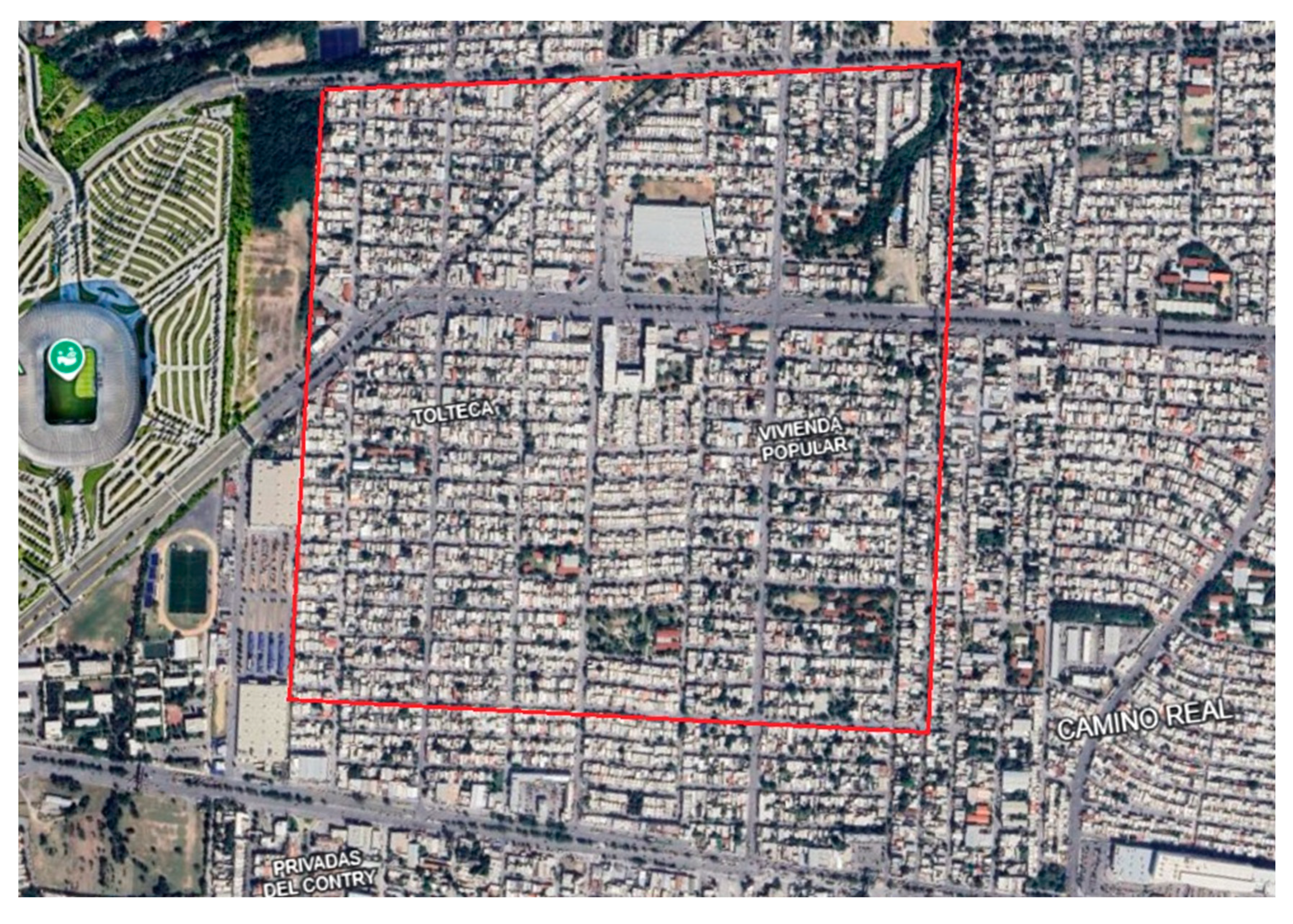
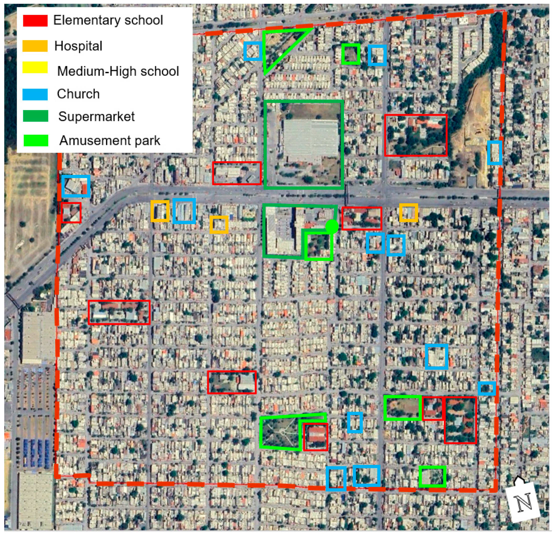
A densely populated representative region of the Monterrey metropolitan area (MMA) was carefully digitized from satellite imagery. The selected site corresponded to La Pastora, located within the municipality of Guadalupe. The DMS coordinates of the region shown within the green dot in Figure 1 were 25°40′5.5″ N 100°14′4.5″ W.

The estimated population of the mapped region was 11,400, with 3570 low-rise buildings, comprising 173 urban blocks. As shown in Figure 1, the urban blocks were mainly residential, but also included elementary schools, clinics, and recreational centers, which serve as community gathering places.

2.2. Generation of the Urban Model

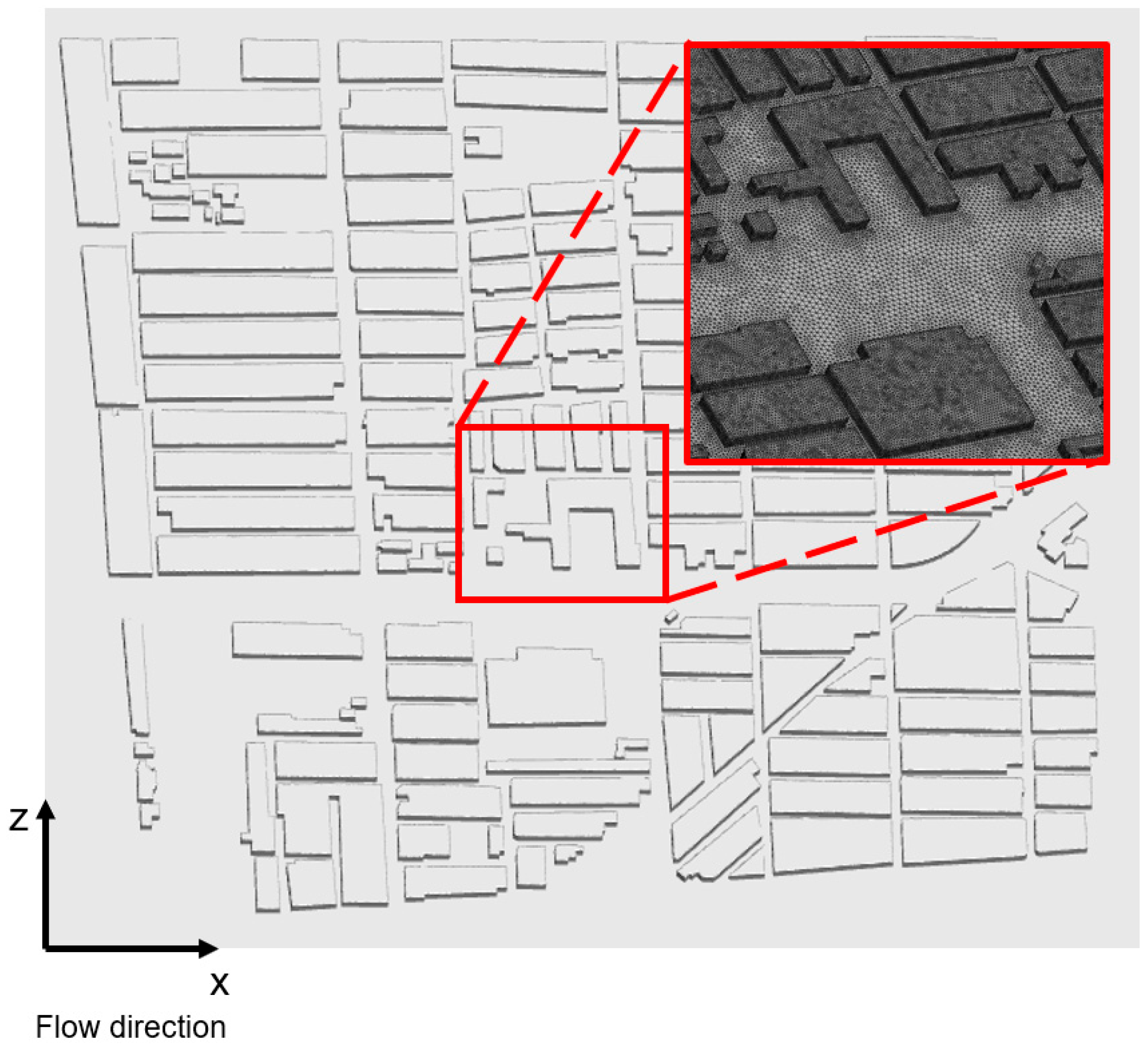
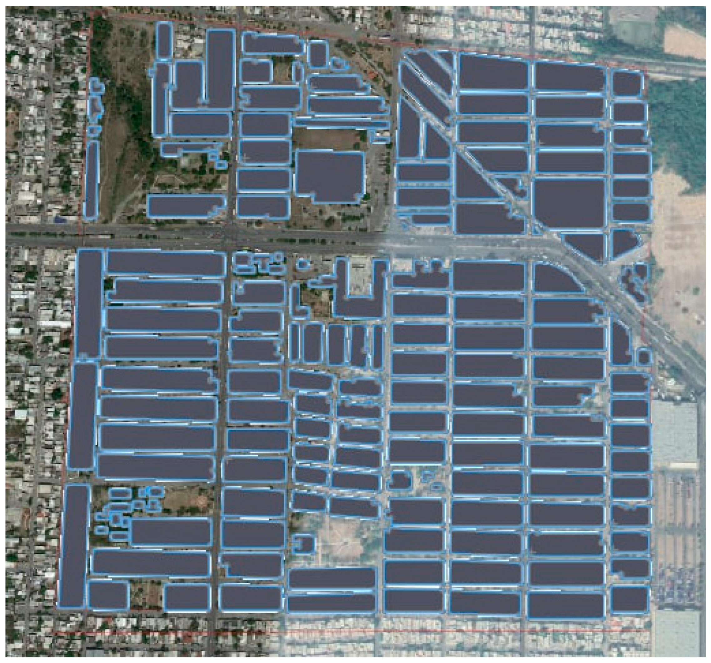
Once the region was selected, the x–y boundaries were defined using the polygon drawing tool in Google Earth. Figure 2 illustrates how a perimeter was delineated to guide the scaling process. Then, as shown in Figure 3, the image was imported into Solidworks^® software (V. 2014.) and used as a template to construct the urban blocks, first as sketches and then as solid volumes, by extruding the block surfaces by 10 m along the normal direction. The distances were scaled properly by measuring, in-site, the longest side of one representative block, using this measure to scale the imported image used as a template. The associated error for this procedure has been estimated to be less than 5% [22]. Other sources of error included the loss of information regarding trees, green fences, and other small-scale complex geometries that were not feasible to reconstruct.

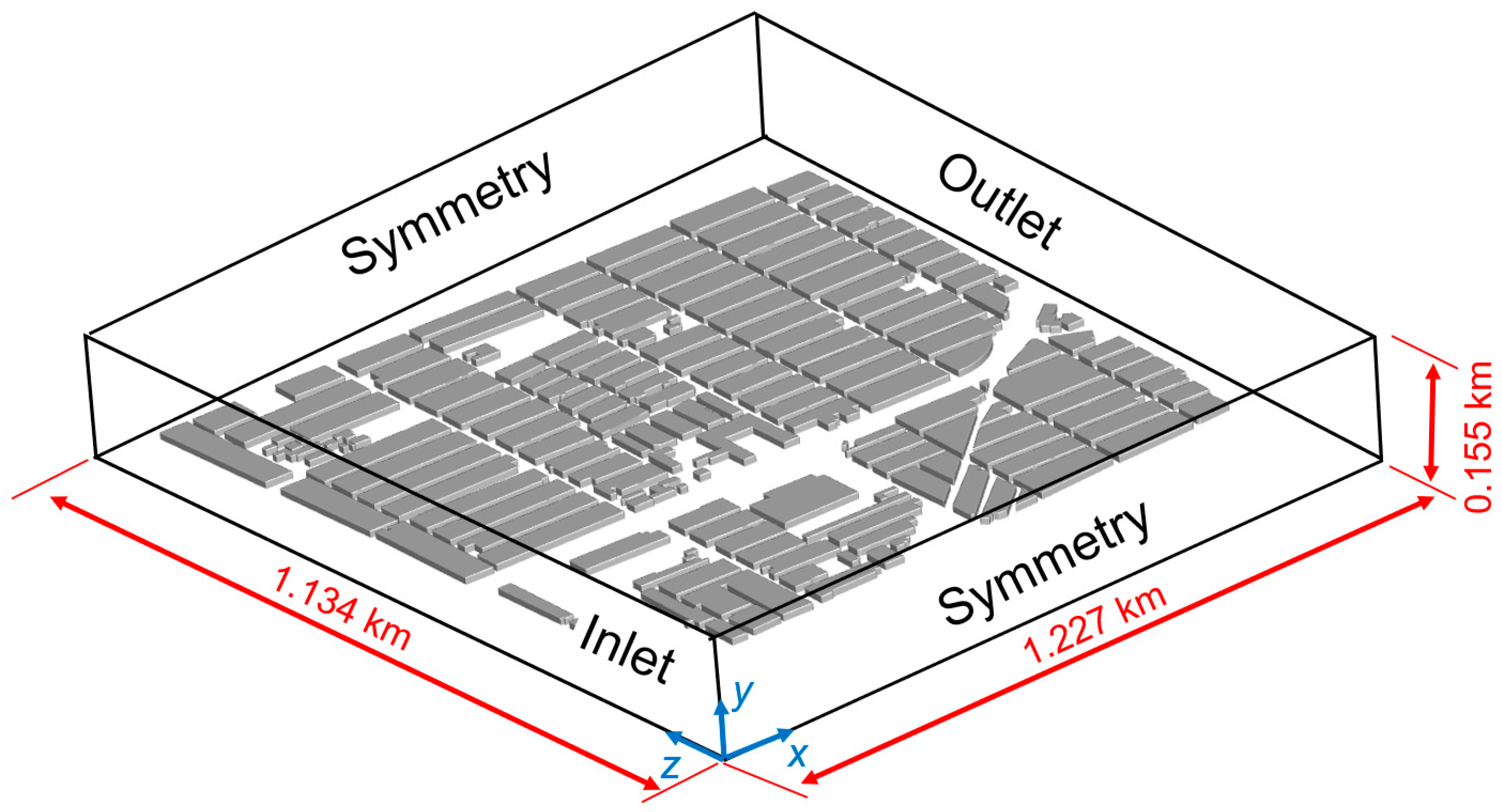
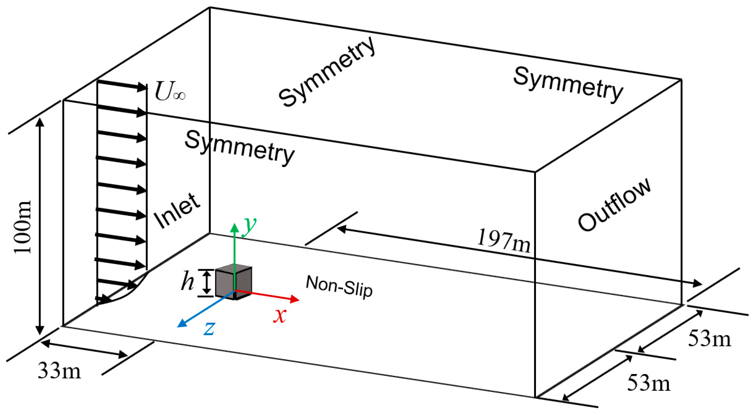
Finally, the computational air domain (1.134 km × 1.227 km × 0.155 km) was generated by subtracting the building volumes using Boolean operations. The resulting air domain is shown in Figure 4.

2.3. Estimation of the Wind Velocities Applied at the Reference Height

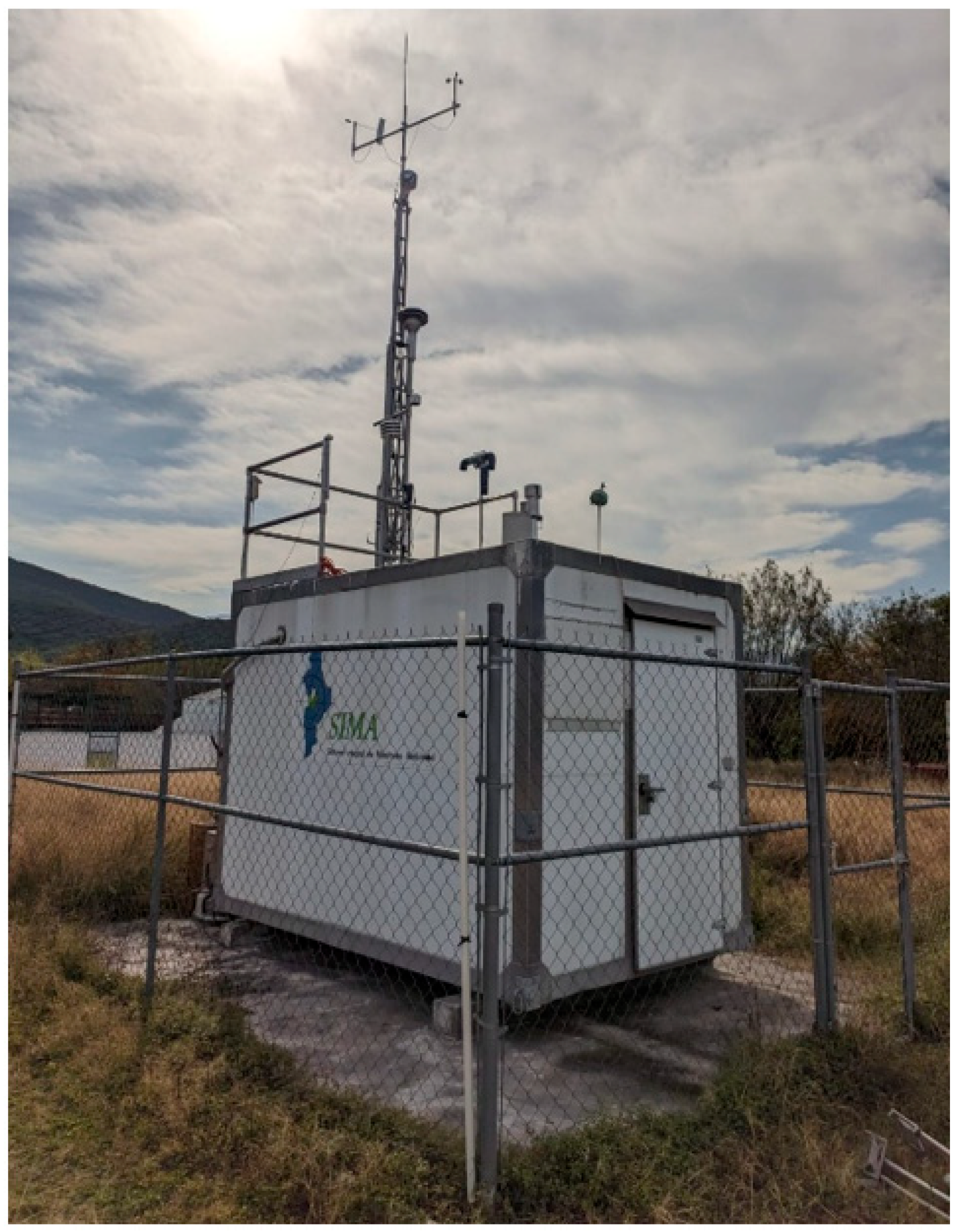
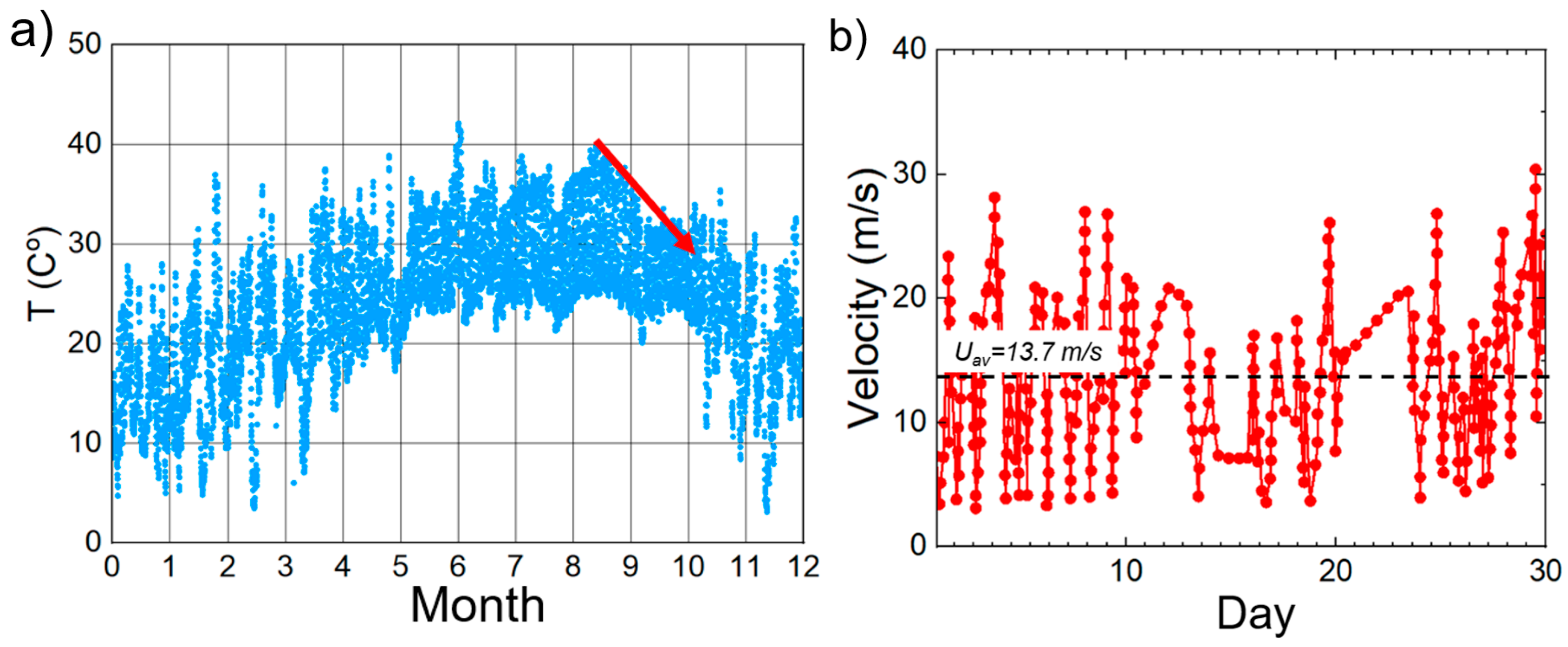
The simulated velocities were acquired from reports from the MMA south weather station, located in the LP area. The velocity signal collected by the anemometer at the reference height h = 10 m, shown in Figure 5, was processed on a monthly basis throughout 2019, by considering pre-COVID19 data to avoid pandemic-related effects. The month of September was chosen as it corresponded to a month with drastic changes in temperatures, related to increases in respiratory diseases, which affected newborn babies and older people in particular. The temperature data for the analyzed year reported by the LP weather station is shown in Figure 6a, with the red arrow pointing out decreases in temperatures from peaks of 40 °C in August to about 20 °C to 33 °C in September. For the selected month, the anemometer signal was processed to obtain the average wind direction, as well as the lowest, peak and average velocities, representing scenarios of low transport, (u_ref = 2.9 m/s), average transport (u_ref = 13.7 m/s) and high transport (air gusts) (u_ref = 30.9 m/s). The velocity data for September are shown in Figure 6b.

The corresponding Reynolds numbers (Re) obtained from Equation (1) were 1.9 × 10⁶, 9.4 × 10⁶ and 21.2 × 10⁶, corresponding to the fully developed turbulent flow regime. The kinematic viscosity was ν = 1.461 × 10⁻⁵ m²/s. In the absence of satellite information on the heights of the buildings (e.g., that contained in the .gis data arrays), the block heights were fixed to h = 10 m. While the different building heights induced uncertainty, especially under low-velocity conditions, in a recent work, the importance metric according to the results of a random forest analysis of the r.m.s. of the building heights indicated low influence regarding the velocity ratios under high-Re conditions [23].

$$Re={\displaystyle \frac{u_{ref}·h}{\nu }},$$

(1)

2.4. Governing Equations and Turbulence Model

At a high Re, the gradient of temperature in the vertical direction is considered negligible, and therefore the air streams are unaffected by buoyancy effects [8,24,25]. The turbulent flow is described by the Navier–Stokes equations, expressed in Cartesian coordinates in Equations (2) and (3). The indexes i,j = 1, 2, 3 represent the x, y and z directions in the Cartesian space, respectively.

$${\displaystyle \frac{\partial {\overline{u}}_i}{\partial x_i}}=0,$$

(2)

$$\rho {\displaystyle \frac{\partial {\overline{u}}_j{\overline{u}}_i}{\partial x_j}}=-{\displaystyle \frac{\partial \overline{P}}{\partial x_i}}+{\displaystyle \frac{\partial }{\partial x_j}}\left[\mu {\displaystyle \frac{\partial {\overline{u}}_i}{\partial x_j}}-\rho \overline{{u^{\mathit{\prime }}}_i{u^{\mathit{\prime }}}_j}\right],$$

(3)

The average Reynolds stress tensor $(-\rho \overline{{u^{\prime }}_i{u^{\prime }}_j})$, which represents the average contributions of the turbulent eddies, is modeled using the turbulent viscosity and the strain rate according to the Boussinesq approximation, described in Equation (4):

$$-\rho \overline{{u^{\prime }}_i{u^{\prime }}_j}={\mu }_t\left({\displaystyle \frac{\partial {\overline{u}}_i}{\partial x_j}}+{\displaystyle \frac{\partial {\overline{u}}_j}{\partial x_i}}\right)-{\displaystyle \frac{2}{3}}\left(\rho k\right){\delta }_{ij}.$$

(4)

In Equation (4), the term k is the turbulent kinetic energy, while µ_t, is the eddy viscosity defined by Equation (5):

$${\mu }_t=\rho C_{\mu }{\displaystyle \frac{k^2}{\epsilon }}.$$

(5)

The closure differential equations for the turbulent kinetic energy k and its dissipation rate ε correspond to the RNG model and are listed in Equations (6) and (7). The details of the theory for this are presented in [26].

$${\displaystyle \frac{\partial \left(\rho k\right)}{\partial t}}+{\displaystyle \frac{\partial \left(\rho k{u}_i\right)}{\partial x_i}}={\displaystyle \frac{\partial }{\partial x_i}}\left[\left(\mu +{\displaystyle \frac{{\mu }_t}{{\sigma }_k}}\right){\displaystyle \frac{\partial k}{\partial x_i}}\right]+\rho \left(P_k-\epsilon \right),$$

(6)

$${\displaystyle \frac{\partial \left(\rho \epsilon \right)}{\partial t}}+{\displaystyle \frac{\partial \left(\rho \epsilon u_i\right)}{\partial x_i}}={\displaystyle \frac{\partial }{\partial x_i}}\left[\left(\mu +{\displaystyle \frac{{\mu }_t}{{\sigma }_{\epsilon }}}\right){\displaystyle \frac{\partial \epsilon }{\partial x_i}}\right]+C_1{\displaystyle \frac{\epsilon }{k}}{P}_k-\alpha {\displaystyle \frac{{\epsilon }^2}{k}}-C_2{\displaystyle \frac{{\epsilon }^2}{k}}.$$

(7)

In Equation (6), the P_k term represents the production of k, and it is described by Equation (8), taking the kinematic turbulent viscosity as υ_t = µ_t/ $\rho$:

$$P_k={\nu }_t\left({\displaystyle \frac{\partial u_i}{\partial x_j}}+{\displaystyle \frac{\partial u_j}{\partial x_i}}\right){\displaystyle \frac{\partial u_i}{\partial x_j}}.$$

(8)

The constant values for the RNG model used in the simulations are listed in

Table 2. Constant values for the k-ε RNG model.

Coefficient	Value	Coefficient	Value
C1	1.42	σε	1.3
C2	1.68	η0	4.38
Cμ	0.0845	β	0.012
σk	1.0	α	1.39

.

According to Blocken et al. [27],the RNG k-ε model has better performance than the standard in replicating recirculation bubbles and velocities in urban models, and has also been applied in the works of Ferreira et al. [28] and Liu et al. [29]. However, as reported by Blocken et al. [7], it is well recognized that conventional RANS models present some drawbacks in regions where the flow is highly decelerated, i.e., regions with impingement, recirculation downstream of windward edges and vortex shedding.

2.5. Boundary Conditions

A logarithmic velocity profile was imposed at the inlet, along with profiles for k and ε, as described in Equations (9)–(11), following the recommendations reported for CFD studies on urban environments [30]. These were implemented as “user defined functions” (UDF) in the ANSYS FLUENT V.18.1 solver.

$$u={\displaystyle \frac{u_f}{{\kappa }_C}}\ln \left({\displaystyle \frac{z+z_0}{z_0}}\right),$$

(9)

$$k={\displaystyle \frac{u_f^2}{\sqrt{C_{\mu }}}},$$

(10)

$$\epsilon ={\displaystyle \frac{u_f^3}{k\left(z+z_0\right)}}.$$

(11)

In the latter relations, u is the velocity component in the main direction, u_f = (τ_w/ $\rho$)^1/2 is the friction velocity, and ${\kappa }_C$ = 0.4 is the von Karman constant. The roughness height z₀ was obtained from Equation (12), in accordance with [31], for the study of low-height urban environments.

$$z_0=1.6{\lambda }_{f}h\left(1-1.67{\lambda }_p\right),$$

(12)

The indexes for plane area λ_p and face area λ_f are defined in Equations (13) and (14), respectively:

$${\lambda }_p={\displaystyle \frac{A_S}{A_T}},$$

(13)

$${\lambda }_f={\displaystyle \frac{A_f}{A_T}}.$$

(14)

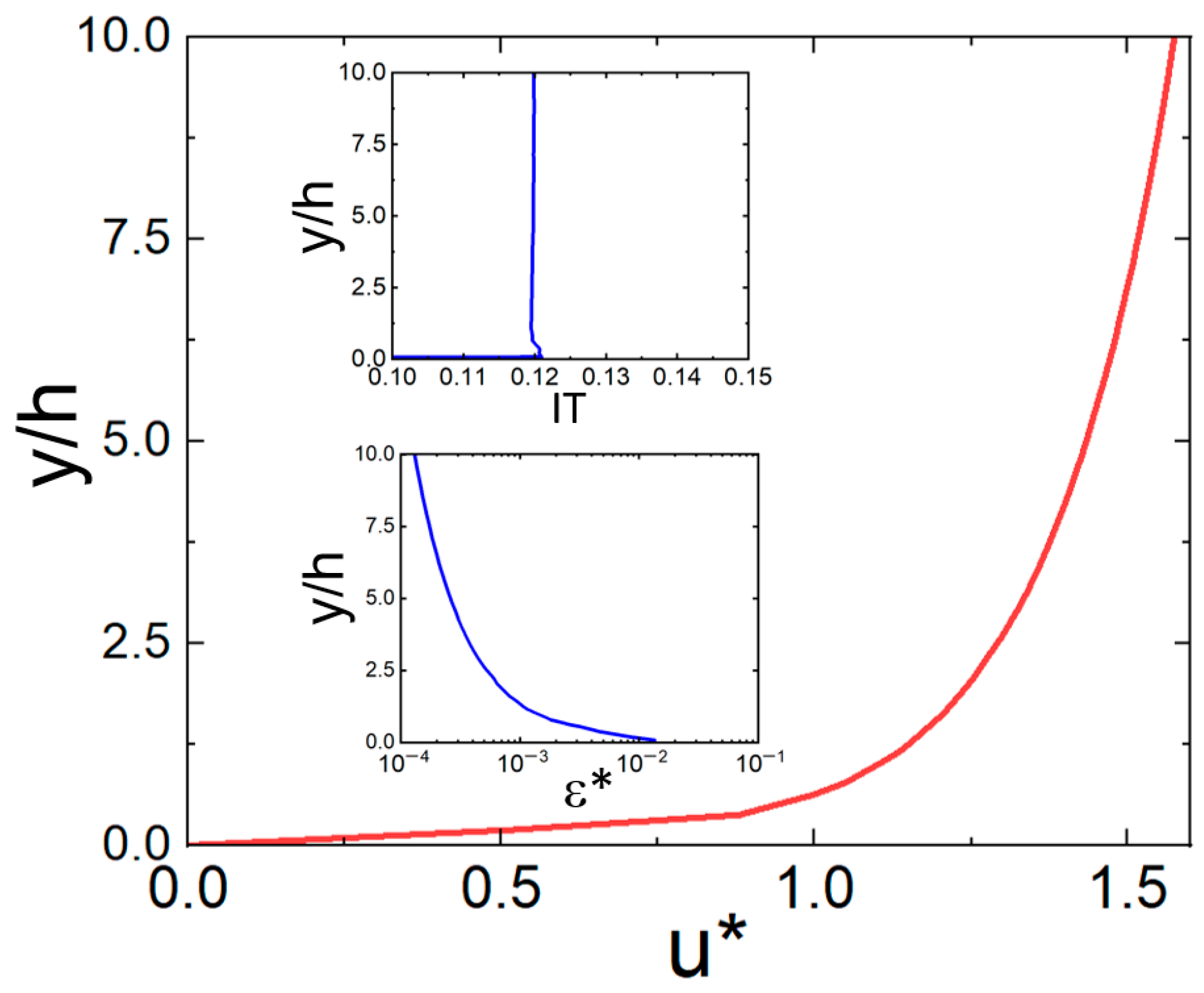
A_T represents the total planar area, A_S is the urban area projected along the normal coordinate, and A_f is the projected building area at the domain inlet. The resulting values were λ_p = 0.40, and λ_f = 7 × 10⁻³, respectively, resulting in z₀ = 0.037 m. A symmetry boundary condition was applied on the lateral and top walls, setting all normal derivatives to zero, that is dψ/dn = 0, where ψ represents any flow variable. The domain outlet was defined as a convective exit by applying the condition dψ/dx = 0. At the ground and building walls, the no-slip boundary condition u_i = 0 was imposed. The minimum distances from the domain boundaries to the first urban elements were adjusted to 10h from the inlet, 5h from the lateral boundaries, and 15h from the outlet, following the guidelines reported in Ref. [32]. The location of the boundary conditions is shown in Figure 4. The SIMPLE pressure– velocity coupling algorithm was implemented in the solver. Second-order pressure discretization and a second-order upwind scheme for the velocity, k and ε terms were applied. All variables were considered converged once they reached the convergence criterion of 1 × 10⁻⁶. For illustrative purposes, Figure 7 shows the normalized x-velocity profile (u* = u/u_ref), turbulence intensity (TI = (2k/3)^1/2/u_ref) and dimensionless dissipation rate (ε* = εh/u_ref³) profiles for u_ref = 13.7 m/s.

2.6. Grid Independence Analysis

To assess the effect of grid spatial resolution on the results, three grids were generated and classified as coarse (7.57 M), medium (16.85 M) and fine (29.68 M), doubling their sizes to avoid false convergence. All grids were composed of tetrahedral cells, which are suitable for complex geometries. The minimum element size was fixed at below 0.56 m near building walls. The grids were generated using the proximity and curvature options in the ANSYS-Meshing module, with several growth ratios. All grids presented average skewness values below 0.23, with maximum values below 0.79, fulfilling the requirements of average values below 0.3 and maximum values below 0.95 stated in the FLUENT user manual for tetrahedral cells (ANSYS, 2009).

Table 3. Sizes and growth characteristics of the grid convergence analysis.

Mesh	N × 106	hmin (m)	Growth Ratio	Iteration Time (s)
Coarse	7.57	0.556	1.20	8
Medium	16.85	0.520	1.08	16
Fine	29.68	0.396	1.08	60

shows some details of the evaluated grids and the simulation times. All simulations were performed using a Dell^® T7600 server with two Intel-Xeon E5-2620 @ 2.0 GHz processors and 64 GB of RAM. The simulations took approximately three days for the coarse grid, six days for the medium grid and twenty days for the fine grid.

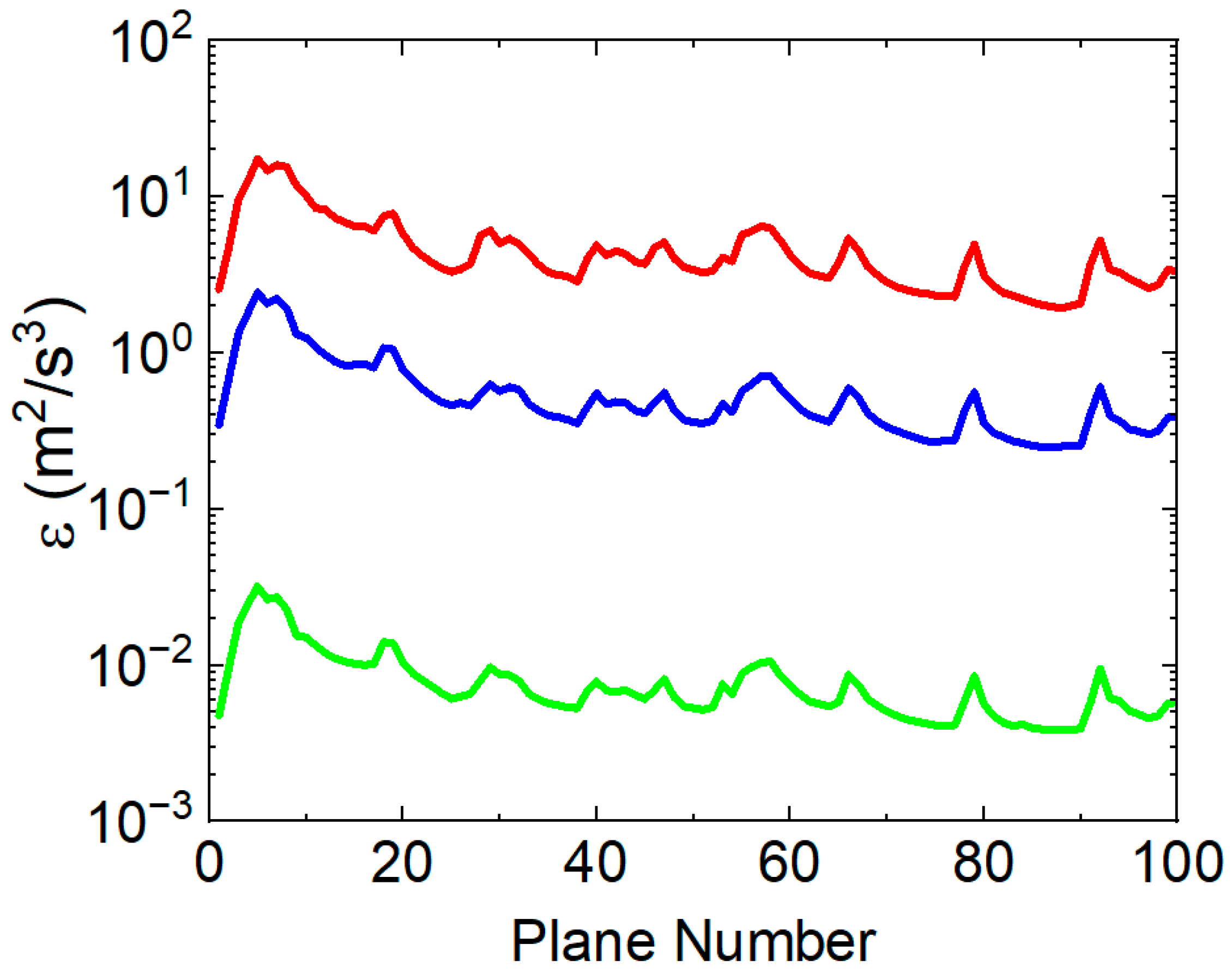
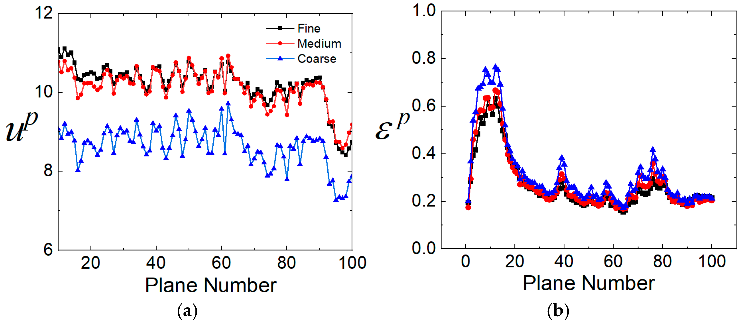
Once the grids were built, the surface-averaged values for x-velocity and dissipation rate (ε) were evaluated using the average velocity of 13.7 m/s as the representative case. For that purpose, one hundred planes perpendicular to the flow were generated to compute plane-averaged values across the entire domain through a custom pseudo-code implemented in the solver. The plane averages of these variables were computed following Equation (15), and the results were plotted in Figure 8a,b.

$${\psi }^p={\displaystyle \frac{1}{ZY}}{\int }_0^Z{\int }_0^Y\psi \left(z,y\right)dzdy.$$

(15)

As shown in Figure 8a,b, for both x-velocity and dissipation rate, the responses of the medium and fine grids were very similar, but the simulation times were significantly higher for the fine grid. The maximum deviations between these plots were below 5% for $u$^P and 10% for ε^p within some regions. Further assessment included the grid convergence index (GCI) method [33,34]. The method was applied to the volume-averaged values of x-velocity 〈u〉^f and the dissipation rate 〈ε〉^f. For that metric, the GCI was 0.014% for the x-velocity and 4.14% for the dissipation rate, respectively. According to this analysis, and considering the simulation times, the medium grid was selected for the remaining velocities. A visual representation of this grid is shown in Figure 9.

2.7. Validation of the Simulation

The performance of the RNG model was validated using data from the turbulent flow over a mounted cube under an atmospheric boundary layer, preserving the same nodal strategy of the medium grid. The height of the cube was fixed at h = 6 m, and the wall distances replicated the wall distance used in the Ref. [35]. This case was chosen to be representative of the expected physics in the most complex urban terrain, that is, flow separation, recirculation, front pressurization, etc. During this analysis, special care was taken to preserve the number of elements in the main flow direction, that is, about 1350 cells, and the same growth ratio.

In addition, the cell type, coupling schemes, spatial discretization orders, and convergence criteria remained unchanged. Figure 10 shows the domain lengths and cube position of the tested case. A logarithmic velocity profile was set at the inlet along with the corresponding profiles for k and ε, in accordance with Equations (9)–(11), described in the main text, taking u_ref = 6 m/s and z₀ = 0.01 m. The lower boundary and the cube surfaces were set as walls where the no-slip condition was imposed, the lateral and upper boundaries were set as symmetries and the rear boundary was set as a velocity outlet.

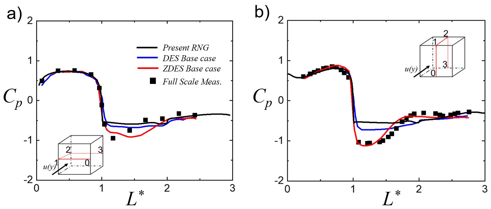
The results for the pressure coefficients, C_P, defined in Equation (16), along the mid-lateral and vertical lines covering the cube faces, as well as their comparison with the data presented in the Refs. [35,36], are presented in Figure 11a,b. Here, L^* = l/h, with l denoting the position along the red arrows shown in detail in both figures. A good agreement is observed in the results for both front and rear face profiles. The differences in the upper walls, especially evident in Figure 11b, may be explained by the limitations of the RNG model to capture the unsteady behavior near the upper separation region, but also the experimental uncertainties arising from full-scale outdoor measurements.

$$C_P=2·{\displaystyle \frac{P-P_{ref}}{\rho u_{ref}^2}},$$

(16)

Another parameter used for validation purposes is the drag coefficient (C_D), defined in Equation (17). For this parameter, F_x is the bulk force in the main direction, resulting from the decomposition of the shear and normal stresses acting on all cube walls, and A_s is the area of the front cube face.

$$C_D={\displaystyle \frac{2F_x}{\rho u_{ref}^2 A_s}},$$

(17)

The predicted value using the present RNG model was 0.97, which matched the value reported in Ref. [37], obtained by LES, and the 0.95 value obtained from the experiments reported in Ref. [38]. It is well recognized that both stress and normal force components define separation strength, reattachment and recirculation extents. Accordingly, the discussed trends based on the simulation methods are considered reasonably valid.

3. Results

3.1. Velocity Analysis Along Several Normal Planes

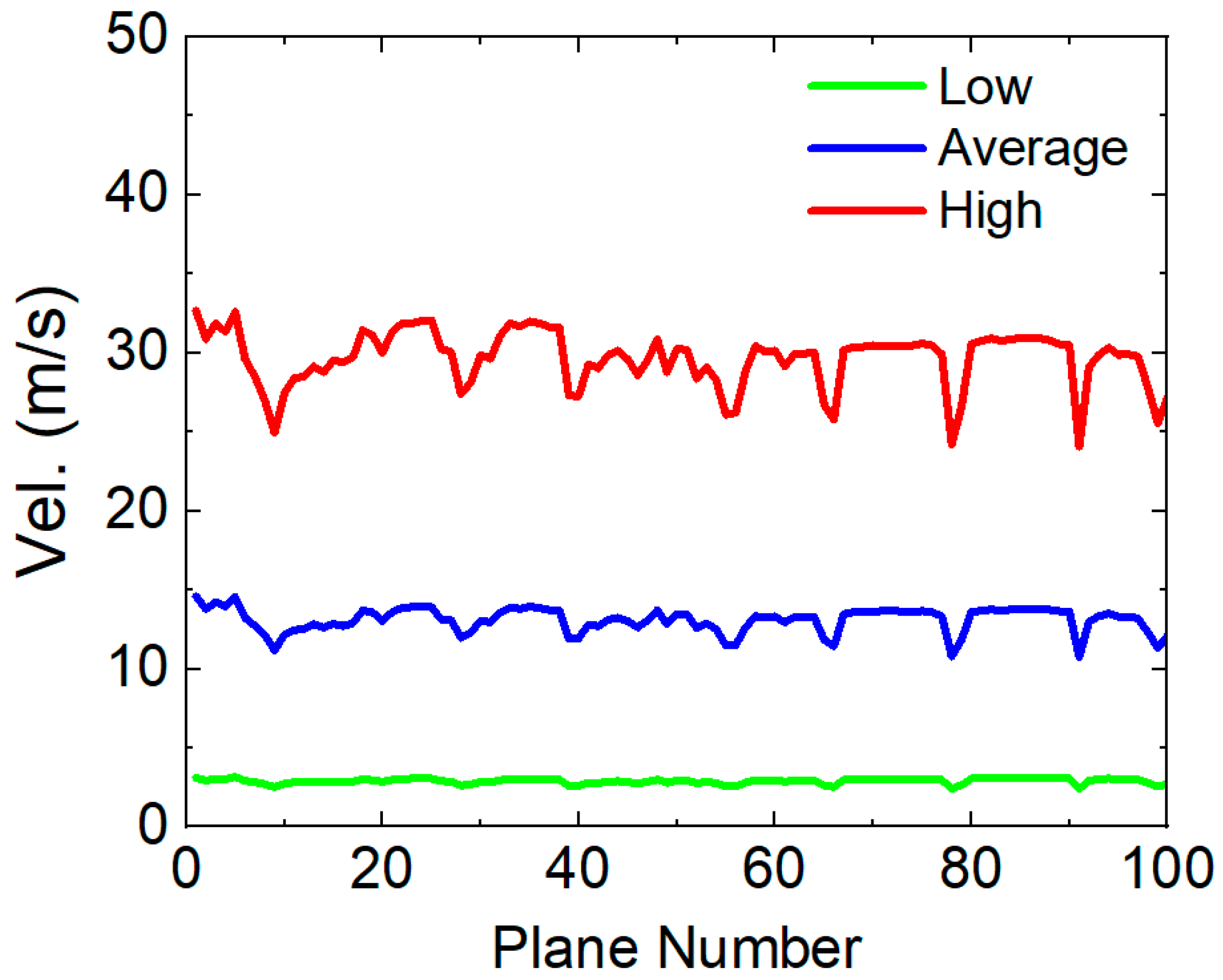
As shown in Figure 12, under high-speed conditions (red line), the flow exhibited a pulsatile irregular behavior, oscillating between 25 m/s and 30 m/s due to urban blocks acting as barriers. At the average speed, the effect was smoothed, reaching almost constant conditions at the lowest reference velocity of u_ref = 2.9 m/s.

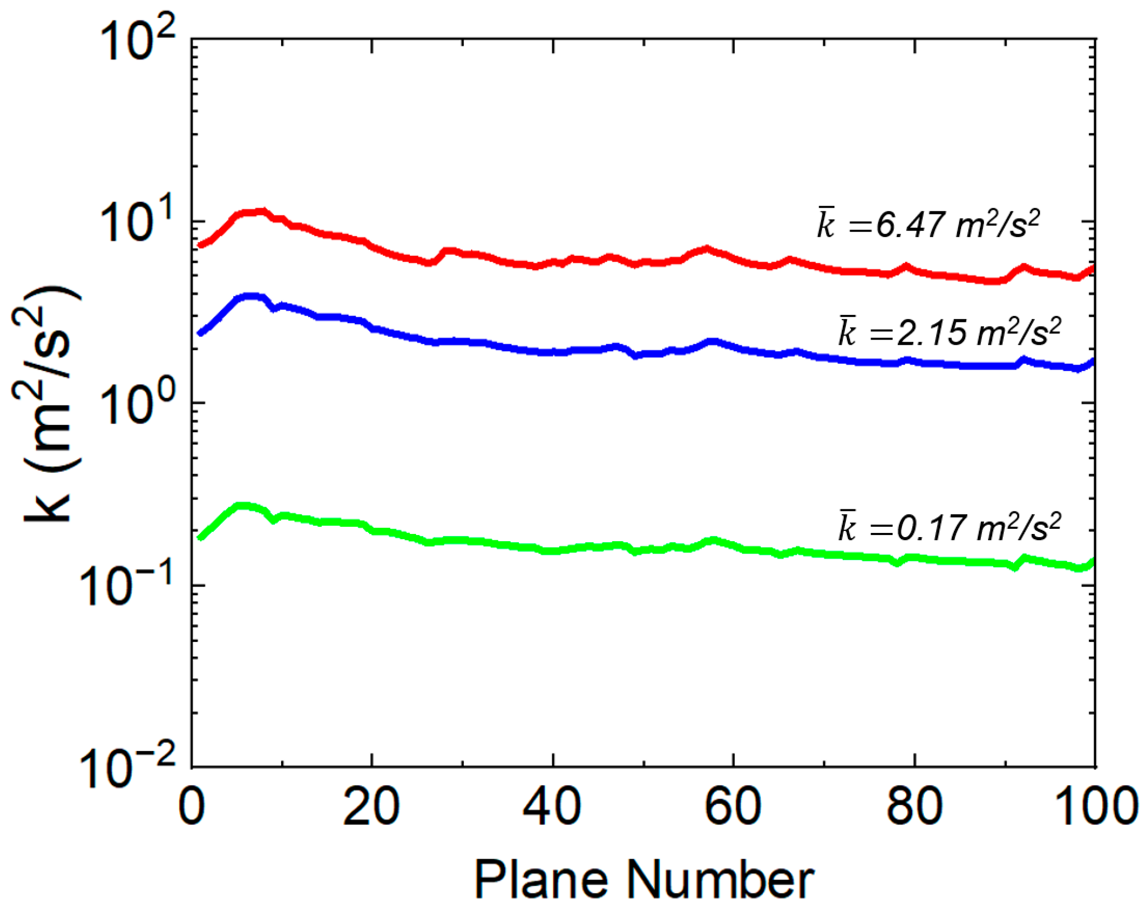
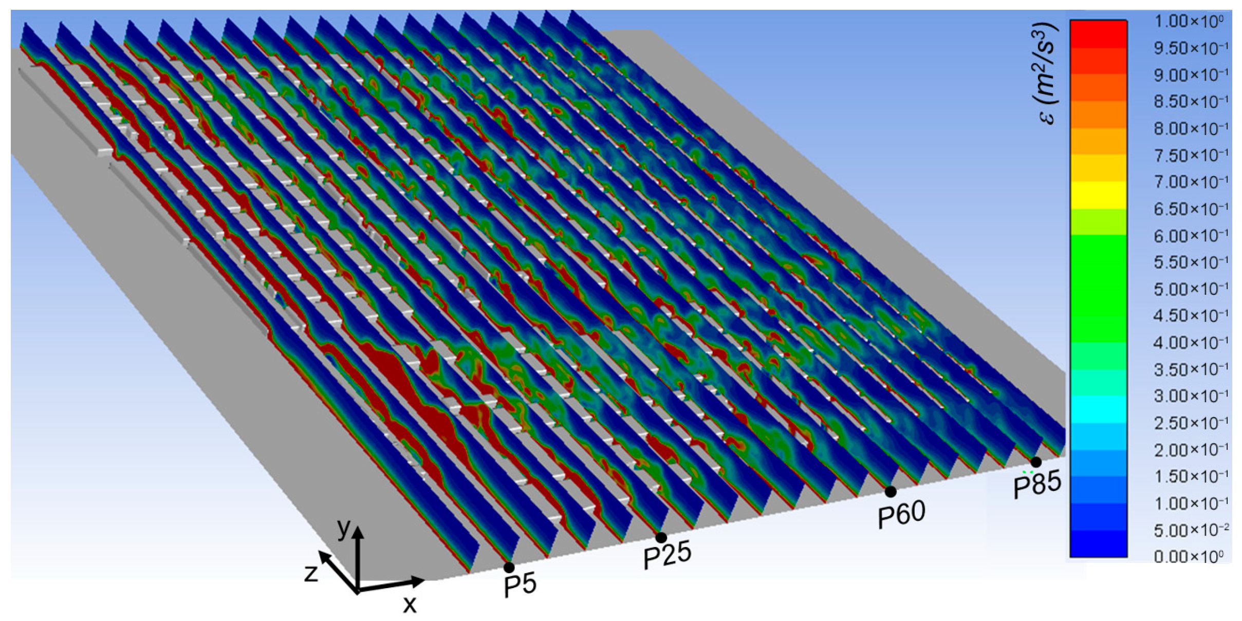
Turbulent kinetic energy (k) is a flow parameter that allows for the quantification of the average energy of the turbulent eddies. As shown in Figure 13, all cases showed almost constant values, but with magnitudes of approximately 38 times larger for the highest u_ref in contrast to the lowest one. Regarding ε, as shown in Figure 14, all signals presented peaks of high dissipation in certain planes, indicating regions that promoted energy losses by friction or viscous dissipation effects, affecting the overall flow transport capability. As shown in Figure 15, these regions surrounded the urban blocks, which have a non-aerodynamic shape, presenting flow separation in their front faces, enhancing energy losses by turbulence dissipation.

3.2. Contours of Velocity in Several x-z Planes

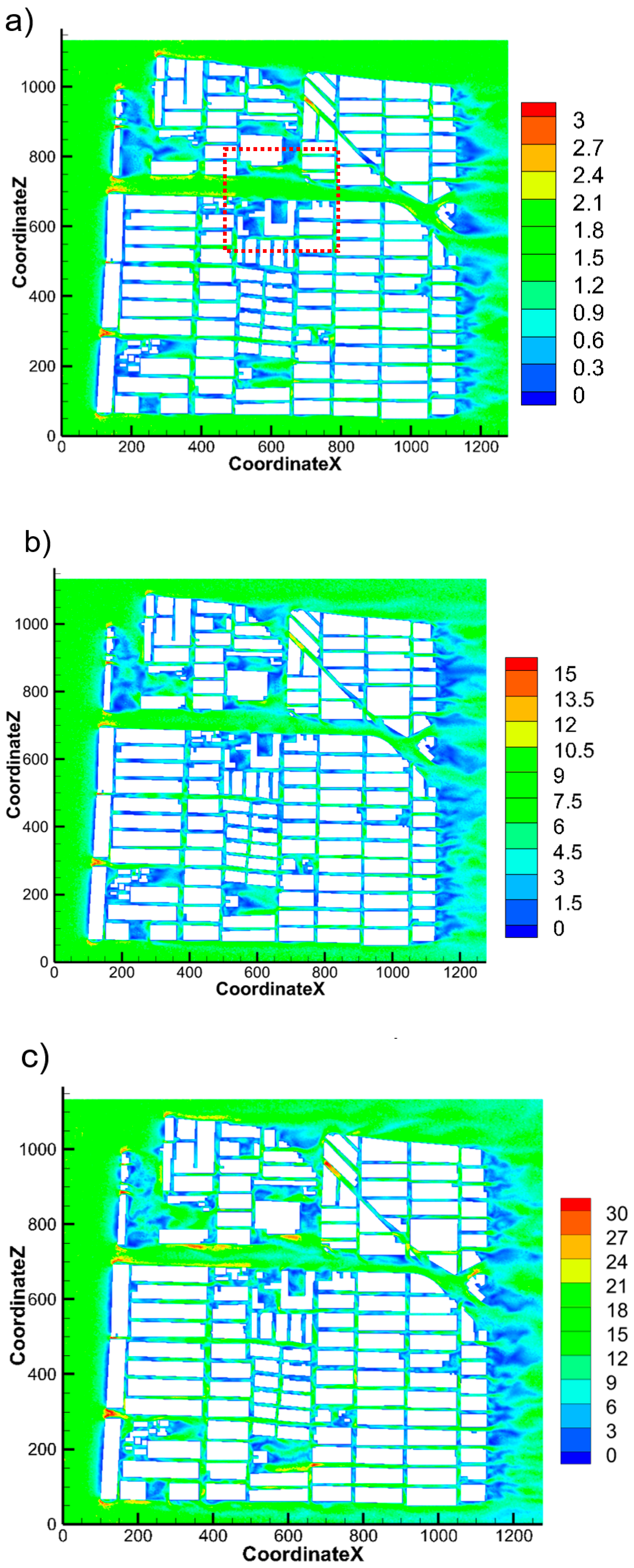
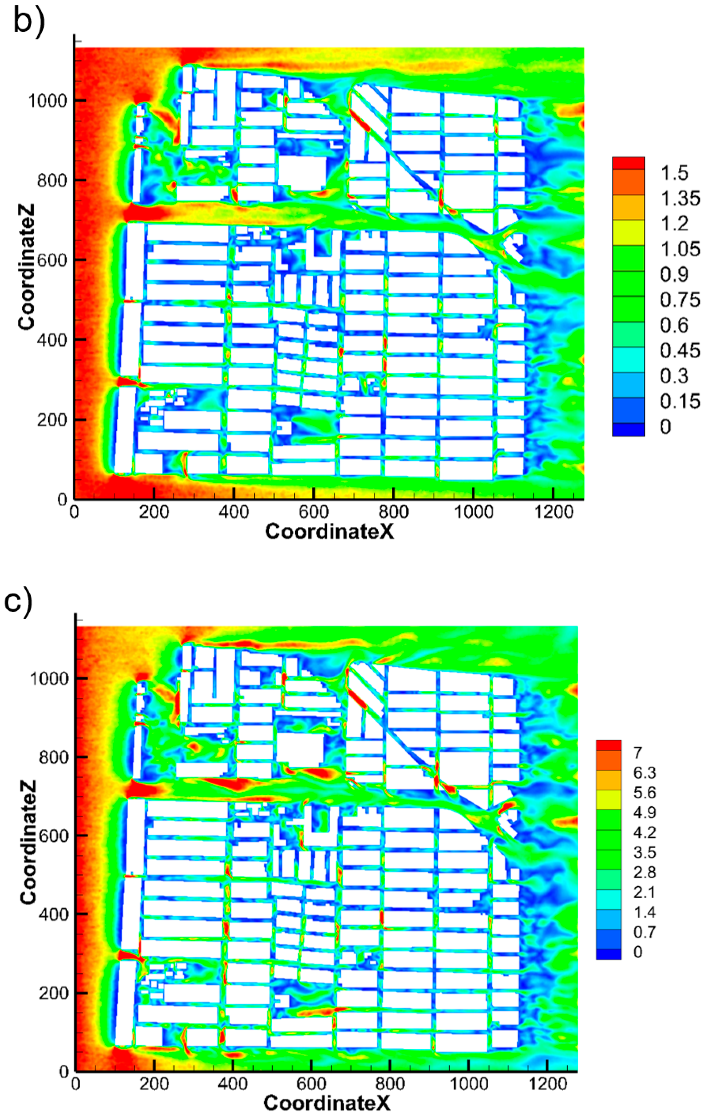
Figure 16a–c show the x-z plane at the pedestrian height h = 2 m for the assessed velocities. Independently of u_ref, the main avenue and parallel percolated paths act as flow channels of high transport, which, in the case of polluted streams, would contribute to pollutant dispersion. On the other hand, between most of the blocks, the velocities are slow, suggesting that if a source of pollution is located there, emitted particles will tend to remain, suggesting zones where trees or green strategies may be applied.

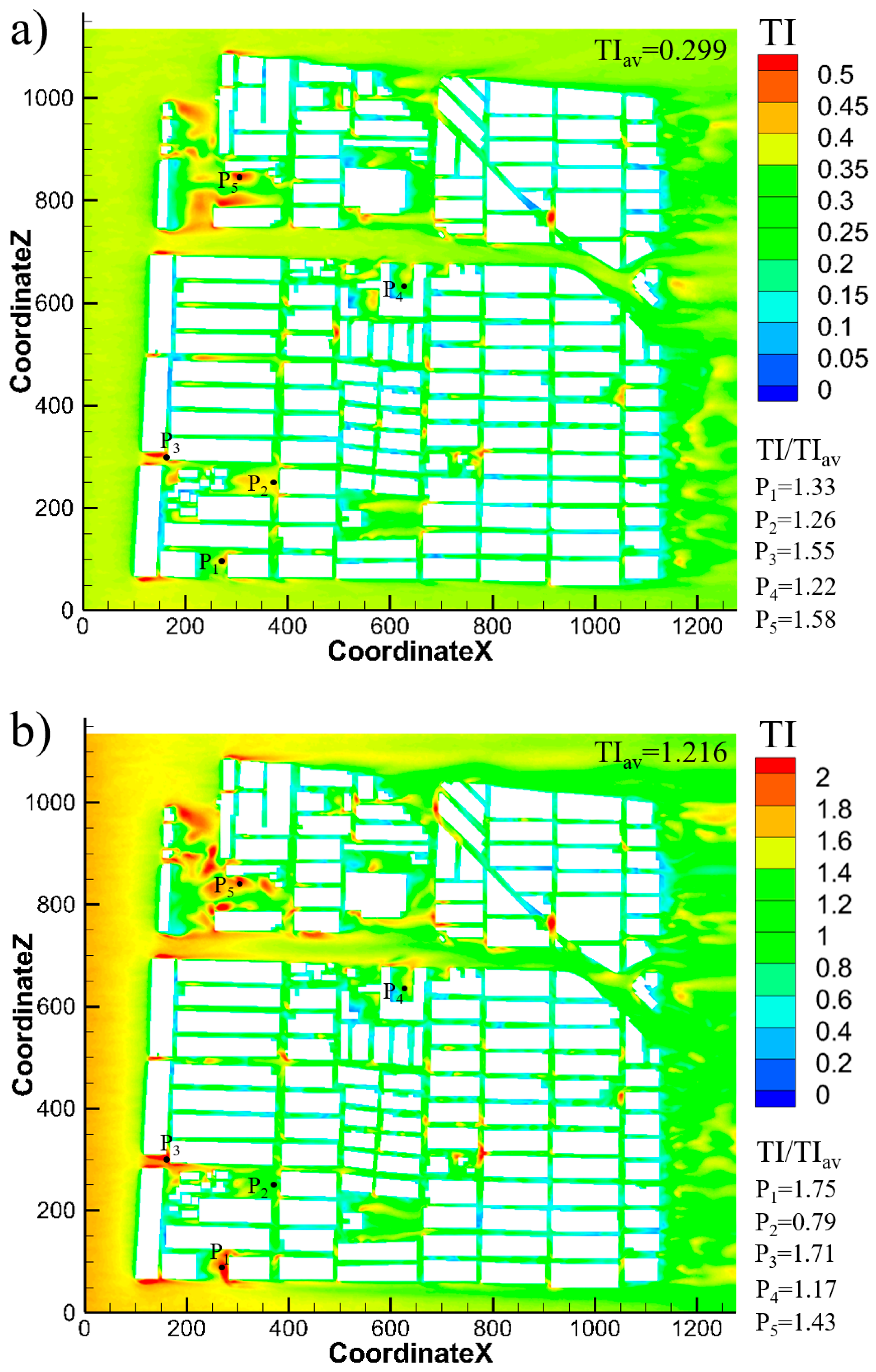
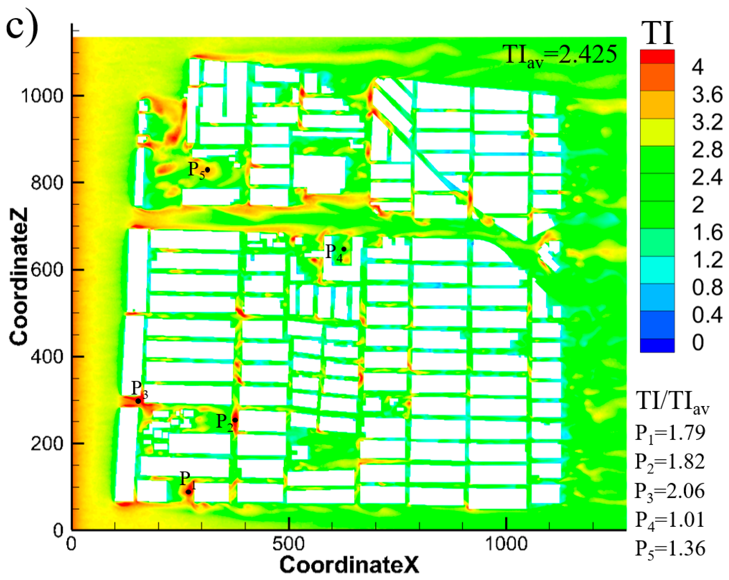
Figure 17a–c show the turbulence intensity (TI) at the pedestrian height. This parameter is an indicator of the strength of the turbulent fluctuations, expressed as a percentage relative to the mean wind flow. As for the velocity, the TI distributions were similar but with different peak levels. Starting from the lowest, u_ref = 2.9 m/s, the higher levels of TI were sequentially doubled at the other velocities. In all cases, the highest turbulence levels were found in open spaces and in the main avenues, where the flow was channeled, and accelerated by contraction. Some local values of the ratio between the TI and the plane-averaged TI are also listed. The irregular trends shown at certain sampling points for a different velocity case indicated that while the accelerations given by gap flows and impingements induce high TI levels, their local values may change, as the flow patterns are highly three-dimensional and complex. For example, for the lowest velocity, and P₂, which is detached near a corner entering a gap, the value was of 1.26, decreasing to 0.79 for the averaged velocity, increasing to 1.79 for the highest velocity.

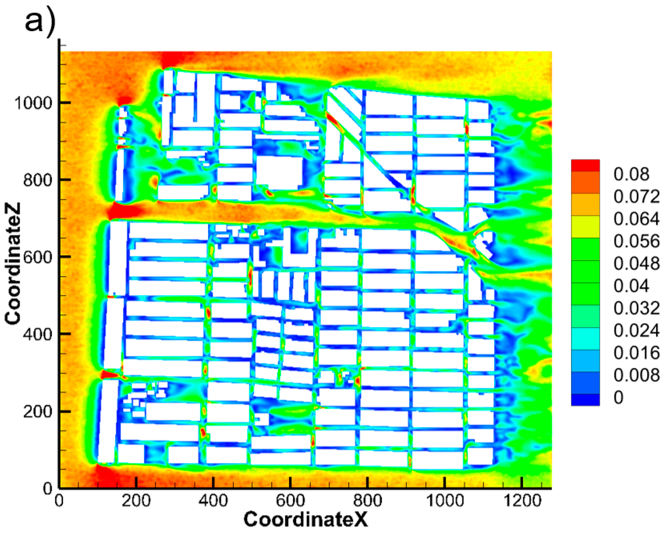
The wall friction coefficient (C_f) maps for each case in the ground plane (y = 0 m) are shown in Figure 18a–c. These were computed using Equation (18), with $\tau$_w referring to the shear stress magnitude on the ground, calculated as ${\tau }_w={\mu \left.{\displaystyle \frac{du}{dy}}\right|}_{y=0}$, with $\mu =1.789\times 10^{-5}kg/(m·s)$ as the dynamic viscosity of air.

$$C_f={\displaystyle \frac{{\tau }_w}{\frac{1}{2}\rho u_{ref}^2}}.$$

(18)

The C_f contours showed that the main friction losses occur in the largest avenue and the lateral interconnected regions, matching some of the high velocity zones at the pedestrian scale. Between blocks, the velocities are slow, and friction is not a significant contributor to flow energy losses.

3.3. Flow Analysis over Several x–y Planes and Other Parameters of Interest

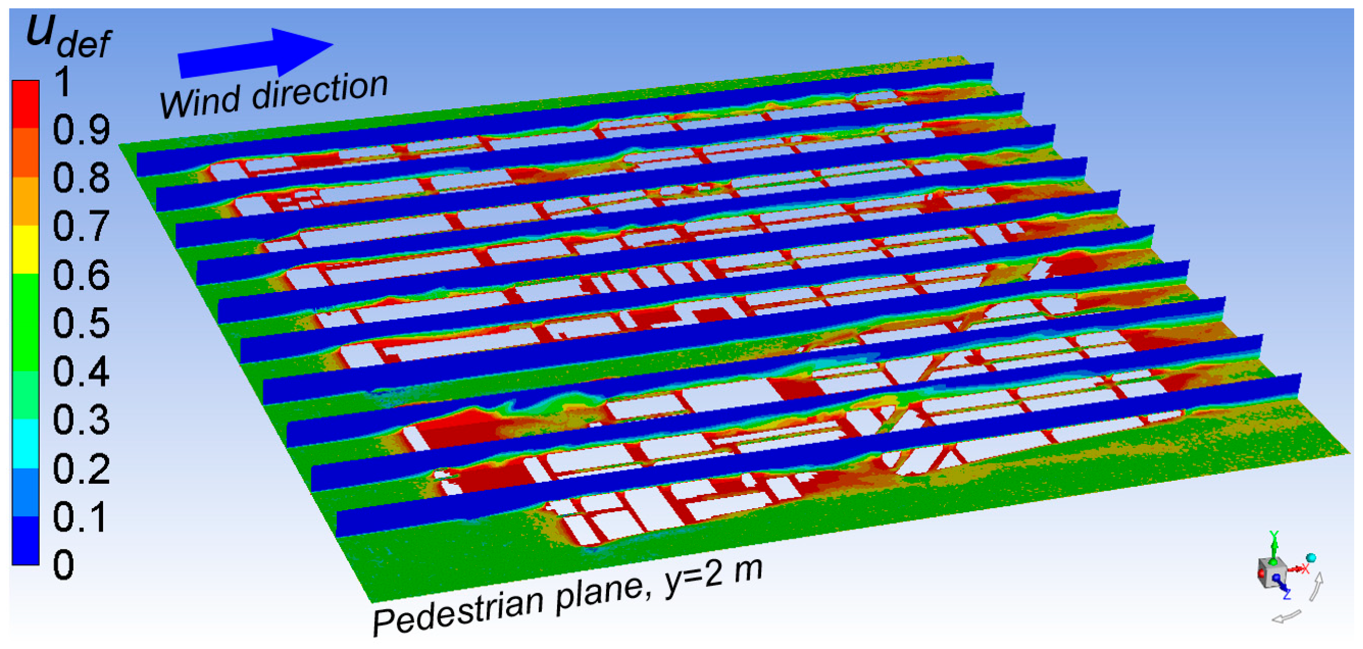
Additional insight into the recirculation regions of the urban blocks is provided by means of the velocity deficit, u_def, using Equation (19), where “u” denotes the streamwise velocity component. As shown in Figure 19, the largest velocity deficits occur downstream of the urban blocks, coinciding with open areas where wakes can fully develop. In the inter-block spaces, the low-velocity cavity flows also generate high u_def.

$$u_{def}={\displaystyle \frac{u_{ref}-u}{u_{ref}}}.$$

(19)

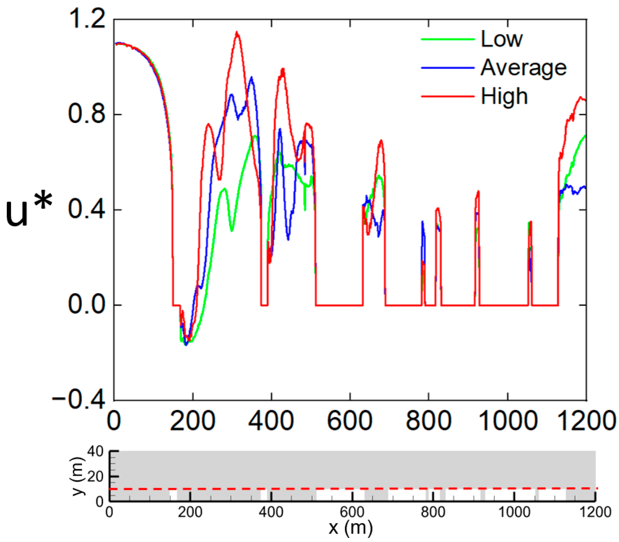
To explore wake recovery lengths, a plot of the normalized velocity was generated along the line at y = 10 m, extracted from the x–y plane located at z = 840 m. As shown in Figure 20, the highest recovery levels occurred downstream of the first two isolated blocks, within the ranges 200 m < x < 350 m and 400 m < x < 500 m. In the remaining gaps, the wakes were more confined, and the profiles displayed a pulsatile pattern resulting from the cavity flows.

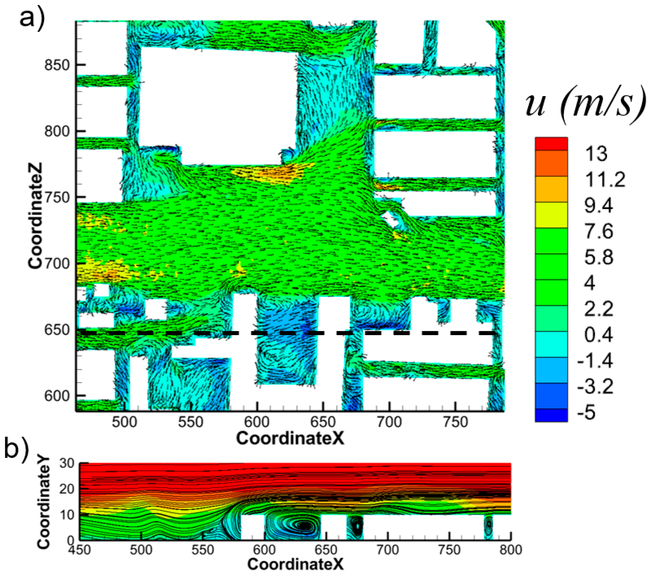
Additional details based on velocity vectors in a representative region are shown in Figure 21a. This region corresponds to the dashed square in Figure 16a, and it is composed of an open space and urban blocks connected laterally to the largest avenue. A high-velocity stream, with vectors of approximately 7.6 m/s, is observed passing through this region and feeding the adjacent lower plaza, where counter-rotating eddies are clearly formed. Other relevant flow features include flow detachment and acceleration at the corners of several blocks—visible in the red-highlighted regions—as well as stream collisions and gap-flow accelerations. From the vertical x–y plot extracted along the dashed line in Figure 21b, both the impingement of the boundary layer and the characteristics of the cavity flows are evident. Similar impingement patterns were reported numerically for a surface-mounted cube in the DNS study by Díaz-Daniel [39].

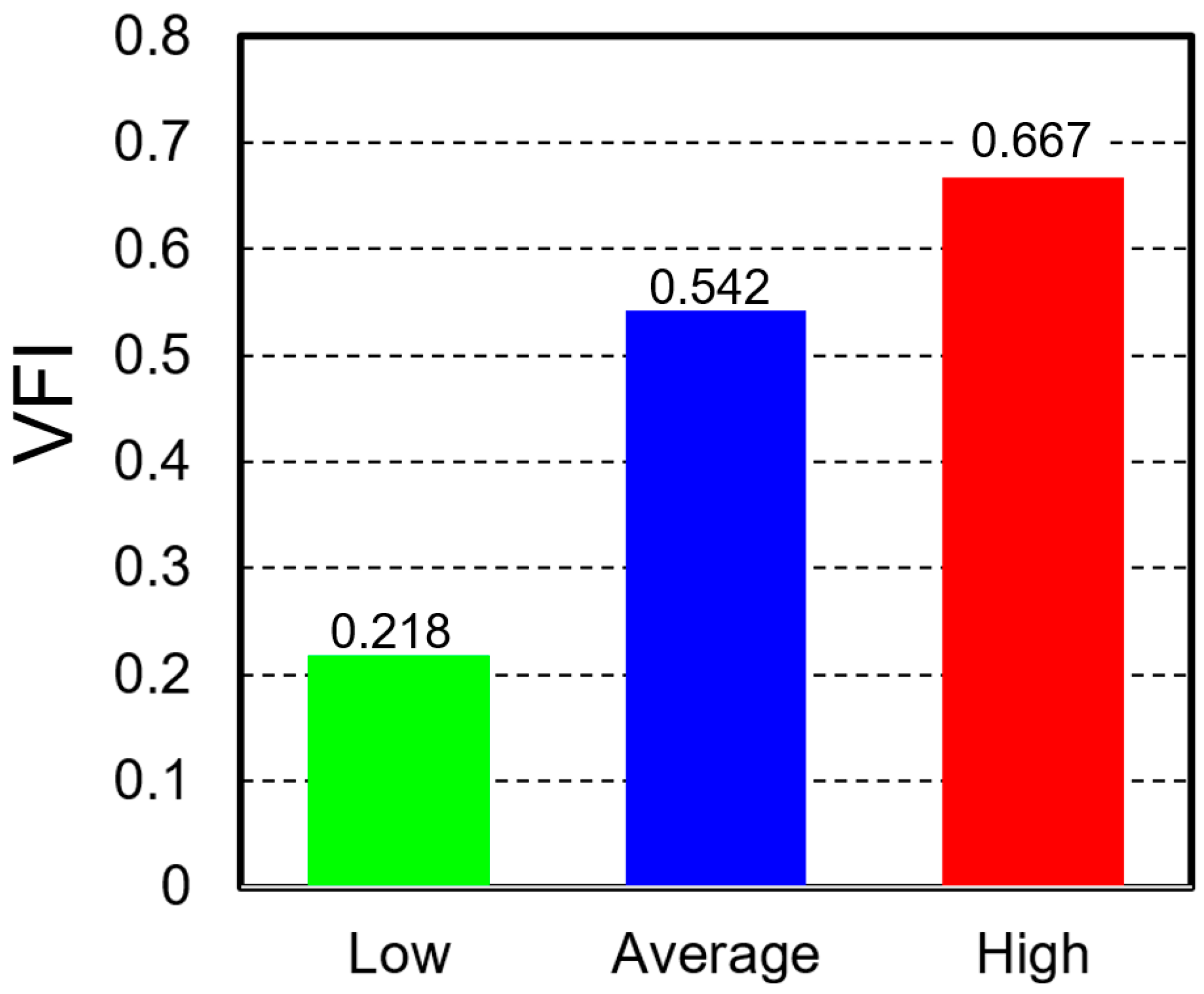
The vertical flushing indicator (VFI) was included to evaluate the vertical momentum induced by the vortices formed between the blocks and, consequently, the ventilation of the cavities. It is defined in Equation (20), where the double-integral operator represents the surface average of the normal velocity component v over the building height x–z plane. As shown in Figure 22, the VFI exhibited strong sensitivity to the Reynolds number, increasing by a factor of 2.5 from the low-velocity conditions to the average-velocity conditions, and by approximately 1.25 between the average- and high-velocity cases, highlighting the complexity of the resulting flow patterns.

$$v^P={\displaystyle \frac{1}{ZX}}{\int }_0^Z{\int }_0^{X}vdzdx,VFI=100\times {\displaystyle \frac{v^P}{u_{ref}}}.$$

(20)

4. Conclusions

The CFD analysis, using the RNG k-ε model, of the turbulent patterns of a representative region of the Monterrey metropolitan area has been performed. The resolved domain was located inside La Pastora district and covered a surface of 1.134 km × 1.227 km, populated by about 11,400 inhabitants. The inlet velocities were processed from the reports of a local weather station and resulted in a Reynolds number range from 1.9 × 10⁶ to 21.2 × 10⁶, corresponding to the fully developed turbulence regime. Results showed that the mean velocity patterns were preserved independently of the Reynolds number and were characterized by regions of high velocity in the main avenues, feeding turbulence into the lateral open spaces, as well as other regions of low velocity between urban blocks. In the latter regions, green strategies such as tree planting can be useful to capture the pollution, while in the main avenues, the same strategy may affect the transport of polluted particles. This methodology may be replicable for other urban regions composed of irregular blocks of low heights arranged irregularly over large surfaces areas, such as those commonly found in Latin American countries. In future work, the same methodology will be applied to other locations and cities in order to correlate the flow patterns and turbulence with the amounts of emitted particulate matter detected by weather stations.

References

1. Okada, T.; Iwayama, T.; Murakami, S.; Torimura, M.; Ogura, T. Nanoscale observation of PM2.5 incorporated into mammalian cells using scanning electron-assisted dielectric microscope. Sci. Rep. 2021, 11, 228. [Google Scholar] [CrossRef] [Scilit]
2. Guo, T.; Wang, Y.; Zhang, H.; Zhang, Y.; Zhao, J.; Wang, Q.; Shen, H.; Wang, Y.; Xie, X.; Wang, L.; et al. The association between ambient PM2.5 exposure and the risk of preterm birth in China: A retrospective cohort study. Sci. Total Environ. 2018, 633, 1453–1459. [Google Scholar] [CrossRef] [Scilit]
3. Ricci, A.; Kalkman, I.; Blocken, B.; Burlando, M.; Repetto, M.P. Impact of turbulence models and roughness height in 3D steady RANS simulations of wind flow in an urban environment. Build. Environ. 2020, 171, 106617. [Google Scholar] [CrossRef] [Scilit]
4. Zou, J.; Yu, Y.; Liu, J.; Niu, J.; Chauhan, K.; Lei, C. Field measurement of the urban pedestrian level wind turbulence. Build. Environ. 2021, 194, 107713. [Google Scholar] [CrossRef] [Scilit]
5. Pavageau, M.; Schatzmann, M. Wind tunnel measurements of concentration fluctuations in an urban street canyon. Atmos. Environ. 1999, 33, 3961–3971. [Google Scholar] [CrossRef] [Scilit]
6. Zhao, Y.; Xue, Y.; Mei, S.; Chao, Y.; Carmeliet, J. Enhancement of heat removal from street canyons due to buoyant approaching flow: Water tunnel PIV-LIF measurements. Build. Environ. 2022, 226, 109757. [Google Scholar] [CrossRef] [Scilit]
7. Blocken, B. 50 years of Computational Wind Engineering: Past, present and future. J. Wind Eng. Ind. Aerodyn. 2014, 129, 69–102. [Google Scholar] [CrossRef] [Scilit]
8. Buccolieri, R.; Santiago, J.L.; Martilli, A. CFD modelling: The most useful tool for developing mesoscale urban canopy parameterizations. Build. Simul. 2021, 14, 407–419. [Google Scholar] [CrossRef] [Scilit]
9. Shirzadi, M.; Mirzaei, P.A.; Tominaga, Y. RANS model calibration using stochastic optimization for accuracy improvement of urban airflow CFD modeling. J. Build. Eng. 2020, 32, 101756. [Google Scholar] [CrossRef] [Scilit]
10. Xiaomin, X.; Zhen, H.; Jiasong, W. The impact of urban street layout on local atmospheric environment. Build. Environ. 2006, 41, 1352–1363. [Google Scholar] [CrossRef] [Scilit]
11. Ehi-Eremosele, F.; Maclaine, A.; Osadolor, A.O.; Bilqees, D.M. Effects of Varying Wind Angles and Increasing Concentration on Air Pollutant Dispersion from Cooling Towers to Urban Area using Computational Fluid Dynamics Software. J. Appl. Sci. Environ. Manag. 2022, 26, 1231–1237. [Google Scholar] [CrossRef] [Scilit]
12. Zhang, X.; Weerasuriya, A.U.; Zhang, W.; Tse, K.T.; Lu, B.; Li, C.Y.; Liu, C.H. Pedestrian wind comfort near a super-tall building with various configurations in an urban-like setting. Build. Simul. 2020, 13, 1385–1408. [Google Scholar] [CrossRef] [Scilit]
13. Chaisri, P.; Ponpesh, P. Prediction of PM2.5 Dispersion in Bangkok Pathumwan District Using CFD Modeling. Eng. J. 2022, 26, 1–13. [Google Scholar] [CrossRef] [Scilit]
14. Brozovsky, J.; Radivojevic, J.; Simonsen, A. Assessing the impact of urban microclimate on building energy demand by coupling CFD and building performance simulation. J. Build. Eng. 2022, 55, 104681. [Google Scholar] [CrossRef] [Scilit]
15. Amorim, J.H.; Rodrigues, V.; Tavares, R.; Valente, J.; Borrego, C. CFD modelling of the aerodynamic effect of trees on urban air pollution dispersion. Sci. Total Environ. 2013, 461, 541–551. [Google Scholar] [CrossRef] [Scilit]
16. Moradpour, M.; Afshin, H.; Farhanieh, B. A numerical study of reactive pollutant dispersion in street canyons with green roofs. Build. Simul. 2018, 11, 125–138. [Google Scholar] [CrossRef] [Scilit]
17. Ishihara, T.; Qian, G.W.; Qi, Y.H. Numerical study of turbulent flow fields in urban areas using modified k ε model and large eddy simulation. J. Wind Eng. Ind. Aerodyn. 2020, 206, 104333. [Google Scholar] [CrossRef] [Scilit]
18. Yoshie, R.; Mochida, A.; Tominaga, Y.; Kataoka, H.; Harimoto, K.; Nozu, T.; Shirasawa, T. Cooperative project for CFD prediction of pedestrian wind environment in the Architectural Institute of Japan. J. Wind Eng. Ind. Aerodyn. 2007, 95, 1551–1578. [Google Scholar] [CrossRef] [Scilit]
19. Hussein, A.S.; El-Shishiny, H. Influences of wind flow over heritage sites: A case study of the wind environment over the Giza Plateau in Egypt. Environ. Model. Softw. 2009, 24, 389–410. [Google Scholar] [CrossRef] [Scilit]
20. Blocken, B.; Janssen, W.D.; van Hooff, T. CFD simulation for pedestrian wind comfort and wind safety in urban areas: General decision framework and case study for the Eindhoven University campus. Environ. Model. Softw. 2012, 30, 15–34. [Google Scholar] [CrossRef] [Scilit]
21. Buccolieri, R.; Gatto, E.; Manisco, M.; Ippolito, F.; Santiago, J.L.; Gao, Z. Characterization of Urban Greening in a District of Lecce (Southern Italy) for the Analysis of CO2 Storage and Air Pollutant Dispersion. Atmosphere 2020, 11, 967. [Google Scholar] [CrossRef] [Scilit]
22. Lopes, E.E.; Nogeira, R.E. Proposta Metodológica para Validação de Imagens de Alta Resolução do Google Earth para a Produção de Mapas. In Proceedings of the Anais XV Simpósio Brasileiro de Sensoriamento Remoto–SBSR, Curitiba, PR, Brasil, 30 April 2011–5 May 2026; 2011; pp. 2308–2315. [Google Scholar]
23. Guo, B.; Chen, M.; Zhu, X.; Wang, Z.; Li, L.; Pei, L.; Chen, H.; Chen, P.; Guo, T. Exploring the effect of the architecture morphology on urban ventilation at block scale using CFD-GIS and random forest combined method. Sustain. Cities Soc. 2025, 122, 106241. [Google Scholar] [CrossRef] [Scilit]
24. Lauriks, T.; Longo, R.; Baetens, D.; Derudi, M.; Parente, A.; Bellemans, A.; van Beeck, J.; Denys, S. Application of Improved CFD Modeling for Prediction and Mitigation of Traffic-Related Air Pollution Hotspots in a Realistic Urban Street. Atmos. Environ. 2021, 246, 118127. [Google Scholar] [CrossRef] [Scilit]
25. Vervoort, R.; Blocken, B.; van Hooff, T. Reduction of particulate matter concentrations by local removal in a building courtyard: Case study for the Delhi American Embassy School. Sci. Total Environ. 2019, 686, 657–680. [Google Scholar] [CrossRef] [Scilit] [PubMed]
26. Yakhot, V.; Orszag, S.A.; Thangam, S.; Gatski, T.B.; Speziale, C.G. Development of turbulence models for shear flows by a double expansion technique. Phys. Fluids A Fluid Dyn. 1992, 4, 1510–1520. [Google Scholar] [CrossRef] [Scilit]
27. Blocken, B.; Stathopoulos, T.; Carmeliet, J.; Hensen, J. Application of computational fluid dynamics in building performance simulation for the outdoor environment: An overview. J. Build. Perform. Simul. 2011, 4, 157–184. [Google Scholar] [CrossRef] [Scilit]
28. Ferreira, A.D.; Sousa, A.C.M.; Viegas, D.X. Prediction of building interference effects on pedestrian level comfort. J. Wind Eng. Ind. Aerodyn. 2002, 90, 305–319. [Google Scholar] [CrossRef] [Scilit]
29. Liu, S.; Pan, W.; Zhao, X.; Zhang, H.; Cheng, X.; Long, Z.; Chen, Q. CFD simulations of wind distribution in an urban community with a full-scale geometrical model. Build. Environ. 2018, 117, 11–23. [Google Scholar] [CrossRef] [Scilit]
30. Hargreaves, D.M.; Wright, N.G. On the use of the k–ε model in commercial CFD software to model the neutral atmospheric boundary layer. J. Wind Eng. Ind. Aerod. 2007, 95, 355–369. [Google Scholar] [CrossRef] [Scilit]
31. Shen, C.; Shen, A.; Cui, Y.; Chen, X.; Liu, Y.; Fan, Q.; Chan, P.; Tian, C.; Wang, C.; Lan, J.; et al. Spatializing the roughness length of heterogeneous urban underlying surfaces to improve the WRF simulation-part 1: A review of morphological methods and model evaluation. Atmos. Environ. 2022, 270, 118874. [Google Scholar] [CrossRef] [Scilit]
32. Blocken, B. Computational Fluid Dynamics for urban physics: Importance, scales, possibilities, limitations and ten tips and tricks towards accurate and reliable simulations. Build. Environ. 2015, 91, 219–245. [Google Scholar] [CrossRef] [Scilit]
33. Roache, P.J. Perspective: A Method for Uniform Reporting of Grid Refinement Studies. J. Fluids Eng. 1994, 116, 405–413. [Google Scholar] [CrossRef] [Scilit]
34. Celik, I.; Karatekin, O. Numerical Experiments on Application of Richardson Extrapolation with Nonuniform Grids. J. Fluids Eng. Trans. ASME 1997, 119, 584–590. [Google Scholar] [CrossRef] [Scilit]
35. Haupt, S.E.; Zajaczkowski, F.J.; Peltier, L.J. Detached Eddy Simulation of Atmospheric Flow About a Surface Mounted Cube at High Reynolds Number. J. Fluids Eng. 2011, 133, 031002. [Google Scholar] [CrossRef] [Scilit]
36. Richards, P.J.; Hoxey, R.P.; Short, L.J. Wind pressures on a 6m cube. J. Wind Eng. Ind. Aerodyn. 2001, 89, 1553–1564. [Google Scholar] [CrossRef] [Scilit]
37. da Silva, B.L.; Sumner, D.; Bergstrom, D.J. Revisiting the surface-mounted cube: An updated perspective of the near wake and near-wall flow field. Int. J. Heat Fluid Flow 2024, 106, 109288. [Google Scholar] [CrossRef] [Scilit]
38. Sakamoto, H.; Oiwake, S. Fluctuating Forces on a Rectangular Prism and a Circular Cylinder Placed Vertically in a Turbulent Boundary Layer. J. Fluids Eng. 1984, 106, 160–166. [Google Scholar] [CrossRef] [Scilit]
39. Diaz-Daniel, C.; Laizet, S.; Vassilicos, J.C. Direct numerical simulations of a wall-attached cube immersed in laminar and turbulent boundary layers. Int. J. Heat Fluid Flow 2017, 68, 269–280. [Google Scholar] [CrossRef] [Scilit]
Figure 1. Satellite imaging and representative zones of the LP area. The green dot refers to the GMS coordinates.
Fluids 11 00023 g001
Figure 2. Definition of the perimeter of the modeled region. At the left it is observed the BBVA-Stadium.
Fluids 11 00023 g002
Figure 3. Reconstruction of the urban blocks using the satellite image as a template.
Fluids 11 00023 g003
Figure 4. Dimensions of the air domain and locations of the boundary conditions.
Fluids 11 00023 g004
Figure 5. Measurement station located in the LP area.
Fluids 11 00023 g005
Figure 6. (a) Annual temperature recorded for the LP weather station; (b) velocity measurements made every 2 h.
Fluids 11 00023 g006
Figure 7. Logarithmic profile imposed at the inlet for uref = 13.7 m/s.
Fluids 11 00023 g007
Figure 8. (a) Plane average velocity distribution along 100 x-z planes; (b) turbulence kinetic energy dissipation rate.
Fluids 11 00023 g008
Figure 9. Illustration of the near block nodal distribution.
Fluids 11 00023 g009
Figure 10. Domain for the flow over an isolated cube.
Fluids 11 00023 g010
Figure 11. Pressure coefficients obtained along the horizontal and vertical mid-face lines. DES, ZDES taken from [35,36].
Fluids 11 00023 g011
Figure 12. Profiles of plane-averaged velocity magnitudes. Note that the high value is 30.7 m/s, the average one is 13.7 m/s and the low one is 2.9 m/s.
Fluids 11 00023 g012
Figure 13. Plane-averaged profiles for k.
Fluids 11 00023 g013
Figure 14. Plane-averaged profiles for the turbulence kinetic energy dissipation rate.
Fluids 11 00023 g014
Figure 15. Contour maps for ε at some representative planes for the average-velocity case, shown in a sequence of five.
Fluids 11 00023 g015
Figure 16. Contours of velocity magnitude at the pedestrian height for (a) low uref, (b) average uref, (c) and high uref. Units are in m/s.
Fluids 11 00023 g016
Figure 17. Contours of TI and representative sampling points at the pedestrian height for (a) low uref, (b) average uref, and (c) high uref.
Fluids 11 00023 g017aFluids 11 00023 g017b
Figure 18. Wall friction coefficient maps at the ground for (a) low uref, (b) average uref, and (c) high uref.
Fluids 11 00023 g018aFluids 11 00023 g018b
Figure 19. Deficit of x-velocity for 10 representative x–y planes spaced 100 m apart for the averaged velocity case of uref = 13.7 m/s.
Fluids 11 00023 g019
Figure 20. Normalized streamwise velocity for the planes z = 840 m and y = 10 m.
Fluids 11 00023 g020
Figure 21. (a) Details of velocity vectors for uref = 13.7 m/s at the pedestrian height plane in a representative region. (b) Streamline and contour maps of velocity in the x–y plane.
Fluids 11 00023 g021
Figure 22. Vertical flushing indicator for the representative velocities.
Fluids 11 00023 g022