Abstract
The current study examines the influence of a varying gravity field and its interaction with density stratification. This represents a novel area in baroclinic flow analysis. The classical vortex and internal wave structures in stratified flows are shown to be significantly modified when gravity varies with height. Vortices may shift, stretch, or weaken depending on the direction and strength of gravity variation, and internal waves develop asymmetries or damping that are not present under constant gravity. We examine the influence of gravity variation on the flow of both homogeneous and density-stratified fluids in a channel with topography consisting of a Gaussian obstacle lying at the bottom of the channel. The flow is without inertia, induced by the translation of the top plate. Both the density and gravity are assumed to vary linearly with height, with the minimum density at the moving top plate. The narrow-gap approach is used to generate the flow field in terms of the pressure gradient along the top plate, which, in turn, is obtained in terms of the bottom topography and the three parameters of the problem, namely, the Froude number and the density and gravity gradients. The resulting stream function is a fifth-order polynomial in the vertical coordinate. In the absence of stratification, the flow is smooth, affected rather slightly by the variable topography, with an essentially linear drop in the pressure induced by the contraction. For a weak stratified fluid, the streamlines become distorted in the form of standing gravity waves. For a stronger stratification, separation occurs, and a pair of vortices generally appears on the two sides of the obstacle, the size of which depends strongly on the flow parameters. The influence of gravity stratification is closely coupled to that of density. We examine conditions where the coupling impacts the pressure and the velocity fields, particularly the onset of gravity waves and vortex flow. Only a mild density gradient is needed for flow separation to occur. The influence of the amplitude and width of the obstacle is also investigated.
1. Introduction
In most natural and astrophysical settings, gravity is rarely uniform. From the Earth’s core to stellar interiors, the gravitational field typically varies with position, especially in the vertical direction due to self-gravitating effects. This study extends beyond traditional fluid dynamics. Gravity gradients are common in planetary interiors, stellar atmospheres, and black hole accretion flows; the insight offered here is directly relevant to astrophysicists and geophysicists when observing flow patterns under variable gravitational fields. Such a coupling of gravitational physics with baroclinic fluid behavior causes the potential inference of the gravitational structure from observable flow fields, offering an indirect diagnostic tool in celestial modeling. Gravity variation is often accompanied by density stratification, which is prevalent in a range of flow regimes, such as in the Earth’s atmosphere, oceans, lakes, magmas, and cosmic gas clusters [1,2,3,4]. Density stratification is particularly significant in large-scale movements, such as atmospheric recirculation [5], ocean currents, and double-diffusive convection, influencing climate and weather patterns [6]. In addition, the density stratification of the flow can significantly shape localized motion, transport, and interactions between objects within a fluid.
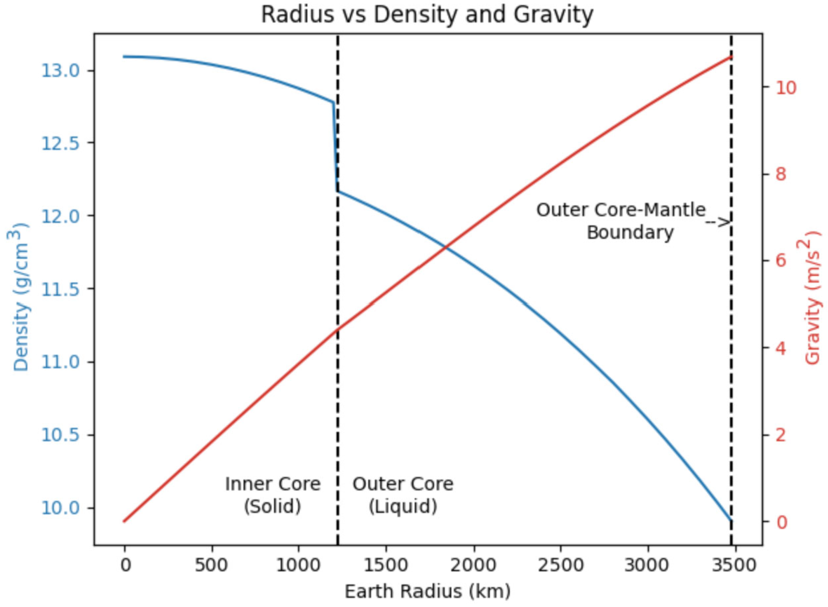
Simultaneously, there are large- and small-scale flows where gravity stratification is also present. For a body with uniform density, the gravitational force inside the celestial body increases linearly with distance from the center. This is because, at any point inside, only the mass enclosed within that radius contributes to the gravitational attraction given by Newton’s law of gravitation. The influence of gravity on the atomic scale is still unknown due to its weak nature, but at the celestial scale, the forces are well defined. For our Earth, the gravity and density variations along the outer core radius are shown by Preliminary Reference Earth model (PREM) data [7], which is reproduced here in Figure 1. In the outer core, the matter is in the liquid state, where convection currents act like a dynamo and produce the magnetic field of our planet. For further details, the reader is referred to Stevenson [8] and Turcotte and Schubert [9].
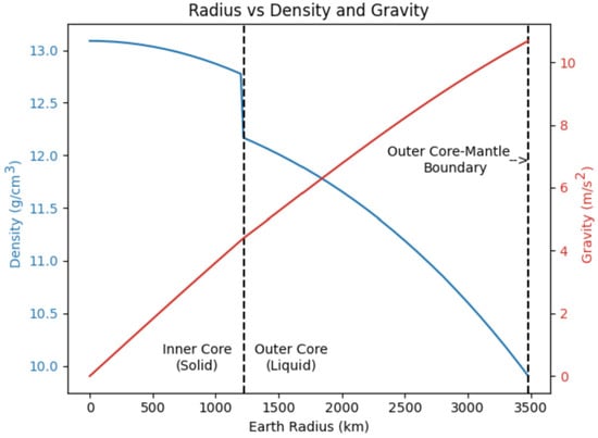
Figure 1.
Variation in the density and gravity acceleration in the core of the Earth. This figure is produced based on the data of Dziewonski et al. [7].
The dual presence in Figure 1 of the density and gravity stratification in the outer core suggests an almost linear trend for both density and gravity; this is certainly the case over shorter distance ranges. The aim of the present study is to elucidate the impact of such a dual presence by examining the flow in a channel of variable topography. The flow in a channel of variable imposed geometry is relevant to a wide range of applications such as static seals formed by compressing two rough metallic surfaces [10], microfluidic systems [11,12], and atmospheric flow [13]. The narrow-gap or lubrication approximation is made, which is an approximation of the boundary-layer equations with negligible inertia at low Reynolds numbers for narrow geometries with slow changes in curvature [14,15,16]. The lubrication approach for non-stratified flow has been widely adopted in the literature, such as for the flow of a Newtonian fluid in a channel with a variable boundary [17]. For a boundary with mild curvature, Tavakol et al. [17] extended the classical lubrication approach by starting with the Stokes equations and considering higher-order terms in a systematic perturbation expansion. The comparison of their analytical high-order results with the experimental results and numerical solutions of the Navier–Stokes equations showed a substantial improvement in the accuracy of the leading-order solution. The work by Tavakol et al. [17] was recently extended by Housiadas and Tsangaris [18] to study a channel with two variable walls, as well as an axisymmetric tube with a variable cross-section. Luberto and de Payrebrune [19] investigated a laminar Couette flow in a channel with theoretically variable geometry, both numerically and experimentally, by placing three square bars or hexagonal bars at the bottom spanning the entire width of the fluid tank.
There are fewer investigations on a channel flow of stratified fluid. One of these pioneering studies is that of Long [13], who investigated the flow induced by the moving obstacle in a channel of a continuous density-stratified fluid. Long [13] proposed a theoretical model for the flow over an obstacle of finite dimensions and found a laminar wave motion if the height of the obstacle is below a certain value; an increase from this height results in closed circulation and negative horizontal velocities. To verify his theory, Long established an experimental device consisting of a long channel with both upper and bottom walls, and an obstacle placed on the bottom wall, which can be moved horizontally along the wall. For small obstacle heights, his experiments verified all the important features predicted by his theory. Later, Long’s [13] theory was employed and extended by multiple other researchers [20,21] for various problems. More recently, Sutherland and Aguilar [22] carried out experiments on the stratified flow over topography and reported on wave generation and mechanisms of boundary-layer separation in the lee of periodic ridges. The recent work of Zaza and Iovieno [23] investigates the influence of coherent vortex rolls on particle motion in unstably stratified channel flow.
Recently, Wang and Khayat [24] examined the flow of a density-stratified fluid in a channel with topography under constant gravity. The flow field was determined using a narrow-gap approach, which was successfully validated against a numerical simulation. While our earlier work focused solely on the influence of density stratification on the flow, the current study focuses on the effect of gravity stratification and its interplay with density stratification. Therefore, the earlier paper forms a baseline study for density-stratified flows over topography. Various assumptions were made, which were validated against a numerical simulation using OpenFOAM (https://www.openfoam.com/). These assumptions included narrow-gap approximation, negligible inertia and convective effects, and the Boussinesq approximation. The study confirmed the plausibility of the theoretical approach in capturing the complex flow structure. Similar assumptions are made in the current study to examine the effect of (positive and negative) gravity gradients on the density-stratified flow. Other similarities between the two studies include the same physical domain and topography. In the present work, we examine the influence of a gravity gradient on the flow of a density-stratified fluid. We thus examine the Couette flow of a fluid with linear density and gravity stratifications in a channel with an obstacle on the bottom stationary plate. This paper is organized as follows: The general formulation and physical domain are described in Section 2. The narrow-gap formulation is elaborated in Section 3. The results of the flow both with and without stratification are given in Section 4. Finally, concluding remarks and discussion are given in Section 5.
2. Physical Domain and General Problem Formulation
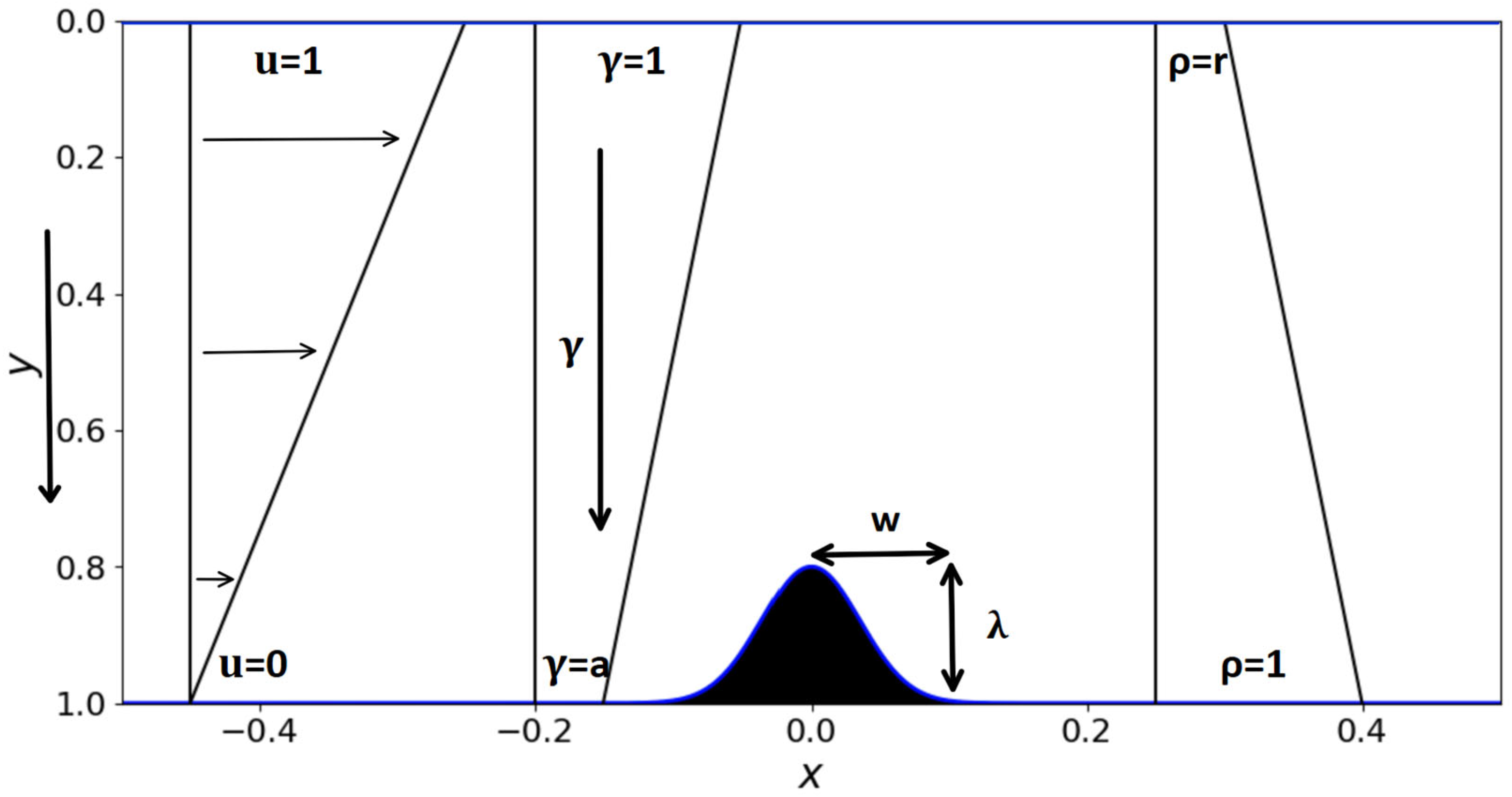
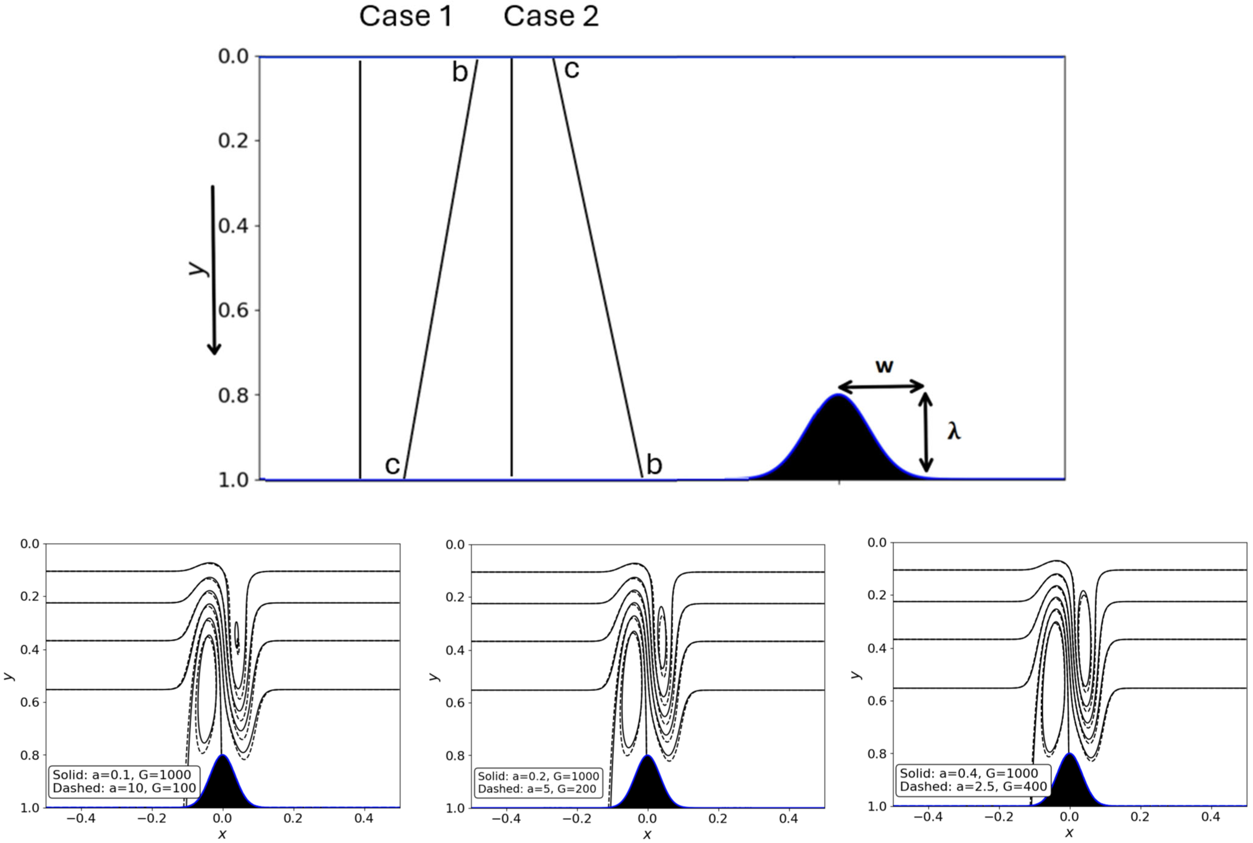
Consider the planar flow in a channel bounded by two rigid boundaries: a straight top plate, translating at a velocity U, and a bottom rigid surface of variable shape, in the form of an obstacle or a depression. The bottom topography is symmetric, with the origin coinciding with the middle of a Gaussian bump. We let ρb and ρt denote the constant density along the bottom and top boundaries.
We choose the channel length L and depth D as the horizontal and vertical length scales, and corresponding velocity scales U and in the horizontal and vertical directions, respectively, where is the aspect ratio. An appropriate choice for L and D is the width and height of the topographic bump. The physical domain is illustrated in Figure 2, where dimensionless notations are used. The coordinate axes are such that the positive x-axis is directed from left to right, and the y-axis points are directed downwards. Gravity is in the positive y direction. Here, u and v denote the dimensionless velocity components scaled by U and in the (x, y) directions, respectively.

Figure 2.
A schematic diagram of the physical domain for a channel with a symmetric obstacle at the bottom boundary. The incoming Couette flow, density, and gravity variations with height are illustrated. All notations are dimensionless. Here, λ = 0.2 and w = 0.05.
The density ρ and pressure p are scaled by the density at the bottom, and , respectively, where g is the acceleration due to gravity. Finally, we denote the top-to-bottom density ratio and bottom-to-top gravity ratios as and , respectively. In addition to , r and a, we have three dimensionless parameters: the Reynolds number, ; the Froude number, ; and the Peclet number, , where and are the dynamic viscosity and stratification agent diffusivity.
The shape of the bottom wall is given by y = h(x), as shown in Figure 2. We are particularly interested in the flow over an obstacle or a depression, so h(x) is a dimensionless Gaussian curve:
where λ and w are the amplitude and half-width of the obstacle (see Figure 2). Note that both the slope and concavity are continuous in x. For an obstacle, the slope is negative upstream of the obstacle (x < 0) and positive downstream (x > 0).
The density and gravity are assumed to vary with height. Whereas decreasing density with height reflects stable stratification, increasing gravity with height mimics the common behavior of self-gravitation inside a celestial body, where gravity is generated by the mass of fluid itself [25].
In this work, dimensionless gravity is assumed to vary linearly with height, so that
The density will also vary linearly with height when the convective effects are neglected, as outlined below.
2.1. Governing Equations and Boundary Conditions
In general, the flow is governed by the Navier–Stokes equations, subject to the Boussinesq approximation for density. An advection–diffusion equation for the stratifying agent (temperature, salinity, or nutrients), incorporating the relationship between the density and the stratifying agent, results in a nonlinear equation governing the density field. The fluid is assumed to be Newtonian and incompressible. The dimensionless conservation of mass and momentum equations for a two-dimensional steady flow are as follows:
and the convective-diffusion equation for density is the following:
Equations (3)–(6) are solved subject to the following boundary conditions at the top and bottom solid surfaces, consisting of adherence and a lack of penetration of the fluid:
and the imposed constant values of the density are as follows:
Clearly, assigning boundary values for the density at the top and bottom plates can be equivalent to imposing a constant temperature along the two boundaries. Alternatively, the heat flux or density gradient can be imposed.
Finally, the conservation of mass produces the following relationship:
2.2. The Flow Far Upstream and Downstream
In addition, boundary conditions are needed both far upstream and downstream of the obstacle, where the flow is assumed to be fully developed. In this case, h(x) ~ 1, v(x, y) ~ 0 and u ~ u(y), and Equations (3)–(6) are reduced to the following:
where . Upon integrating Equation (12) subject to Equation (8), we obtain a linear density profile. In the absence of an imposed pressure gradient, the solution of Equation (11) yields a pressure independent of x, so that the following is calculated:
3. The Narrow-Gap Formulation
The narrow-gap limit is obtained by assuming that ε = H/L << 1. Assuming that Re = O(1), Fr2 = O(ε), and Pe = O(1), all convective and elongation terms in Equations (4) and (5) become negligible to the leading order, yielding the following equations:
Clearly, only three parameters remain, namely G, a, and r. We note that the narrow-gap approximation for fluid without stratification is recovered for incompressible flow (Tavakol et al., 2017) [17].
Upon integrating Equation (12), we recover the linear density profile. In this case,
where is the variable and unknown pressure along the top plate. In particular, the pressure along the bottom is given by the following:
The linear density profile successfully approximates the profile across the interface of a two-layer fluid [26]. Substituting for p from Equation (21) into Equation (17) and integrating this twice, subject to Equation (7), the velocity profile in the channel is the following:
where a prime denotes a derivative with respect to x. The equation for the pressure gradient can be obtained by invoking the conservation of mass relation (Equation (9)), yielding the following:
We observe from Equation (25) that, regardless of the level of density and gravity stratification, the pressure maximum/minimum does not coincide with the mid-obstacle location where since . This is, of course, expected for lubrication flow. However, this is the case as long as G is not too large (otherwise, the middle term becomes negligible).
It is not difficult to see that , which is established from Equations (15) and (22). In this case, the integration of Equation (24) gives the following:
Substituting Equation (24) into Equation (23), we obtain the following:
We note that the velocity profile for a flow without stratification (r = 1) is the same as the classical Couette flow velocity profile [19,27]
Before proceeding further, we determine the velocity component v(x, y) using the continuity equation. Although Equation (3) is first order in y, we expect it to satisfy two boundary conditions, v (x, 0) = v(x, h(x)) = 0. Integrating the continuity equation, and using Equation (7), v(x, 0) = 0, we obtain the following:
The flow field is obtained analytically for any bottom topography. Noting that the flow far upstream is a pure Couette flow under atmospheric pressure, the pressure anywhere is then obtained by integrating Equation (25), subject to Equation (15), yielding the following:
Another important variable is vorticity. In particular, along the moving plate, the vorticity is equal to the wall shear stress(ω). In general,
Another important related quantity worth mentioning is the difference in pressure between the bottom and top boundaries:
Two limit flows naturally emerge in this case. The first is the flow under constant gravity, and the second is the absence of density stratification, which will be discussed shortly.
4. Results
4.1. In the Absence of Density and Gravity Stratifications
The flow in the absence of density and gravity stratification is well established and, therefore, serves as a reference limit that is useful when interpreting complex physics in the presence of stratification. Thus, setting r = a = 1, the flow field is reduced to the following:
Here, G is the only parameter in the problem. In this case, the streamwise pressure gradient is only a function of x, and the velocity component, u, cannot display a change in concavity along the y direction, allowing no possibility of vortex formation. In other words, since for any x, the pressure gradient from Equation (36) is , which is independent of y for any x, thus driving the flow forward and enhancing the plate movement.
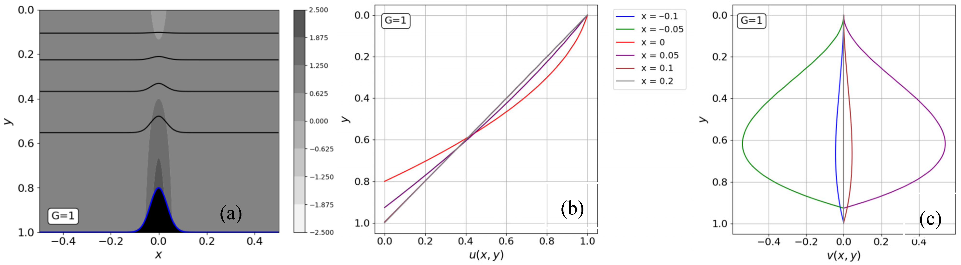
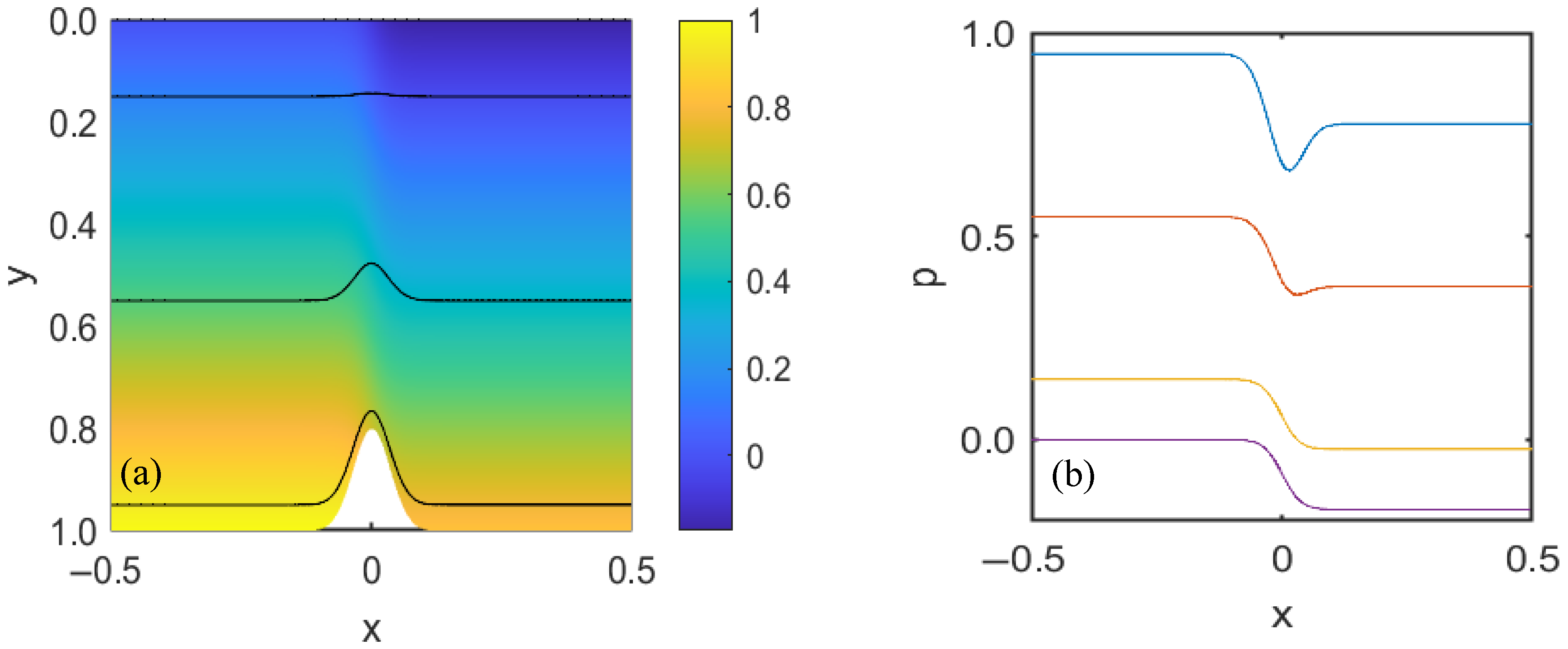
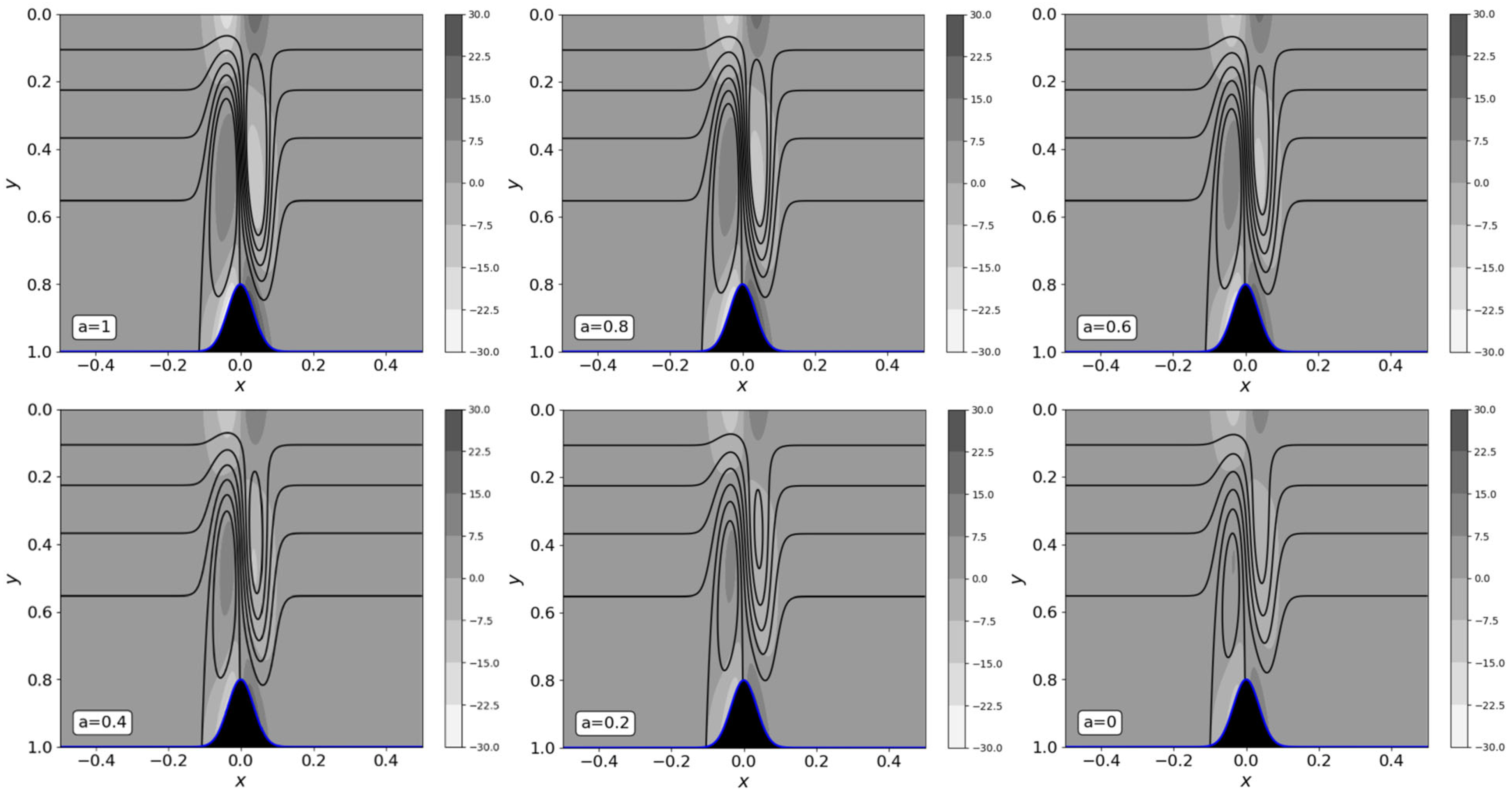
The flow fields for constant density and gravity are shown in Figure 3. The obstacle shape in Equation (1) corresponds to . The streamlines and vorticity contours in Figure 3a show the expected gradual deviation from parallel flow near the top translating plate to the distorted flow near the bottom boundary where the obstacle is located. Figure 3b,c confirm the symmetric and antisymmetric velocity profiles as predicted by Equations (32) and (33), respectively. For , the flow remains Couette and unaffected by the obstacle. Closer to the origin, the flow displays the Couette–Poiseuille characteristic typically predicted by the Reynolds equation for a homogeneous fluid. We note that the v component may appear to be of the same order of magnitude as u (order one in this case), but the true magnitude is of order due to the scaling.
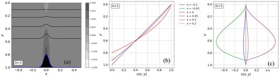
Figure 3.
The flow at G = 1 in the absence of density and gravity stratification (r = a = 1). The (a) flow field and vorticity contours, and the (b) u and (c) v profiles plotted at different values of x (legends common to both u and v) are shown. Here λ = 0.2 and w = 0.05.
Figure 4 illustrates the pressure distribution for the flow in Figure 3. The pressure contours in Figure 4a reflect a decrease in pressure with x and an increase with distance from the top towards the bottom boundary. The pressure gradient is zero upstream and downstream of the obstacle (h = 1). Referring to Equations (34)–(36) and Figure 4b, we can see that the pressure gradient in the x-direction is negative everywhere since h < 1, except along the bottom downstream of the obstacle, where due to the variation in height of the bottom boundary. However, within the interior of the flow, adverse pressure gradients along streamlines develop in the lee of the obstacle, as shown in Figure 3. In a uniform-density fluid, an adverse pressure gradient develops in the expanding flow, leading to deceleration; however, given the absence of stratification, flow reversal cannot occur at the bottom boundary regardless of the bottom’s topography. This is confirmed by the streamwise velocity, u, which is always positive everywhere in the flow. Given the symmetry of the obstacle, the velocity field is also symmetric, as reflected in the symmetric and antisymmetric streamwise and transverse velocity components.
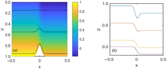
Figure 4.
The flow pressure at G = 1 in the absence of density and gravity stratification (r = a = 1). The (a) pressure distribution and (b) pressure along streamlines starting at far-away upstream heights of y = 0.15 (purple), 0.55 (yellow), 0.95 (red), and along the bottom surface (blue) are shown. Here, λ = 0.2 and w = 0.05.
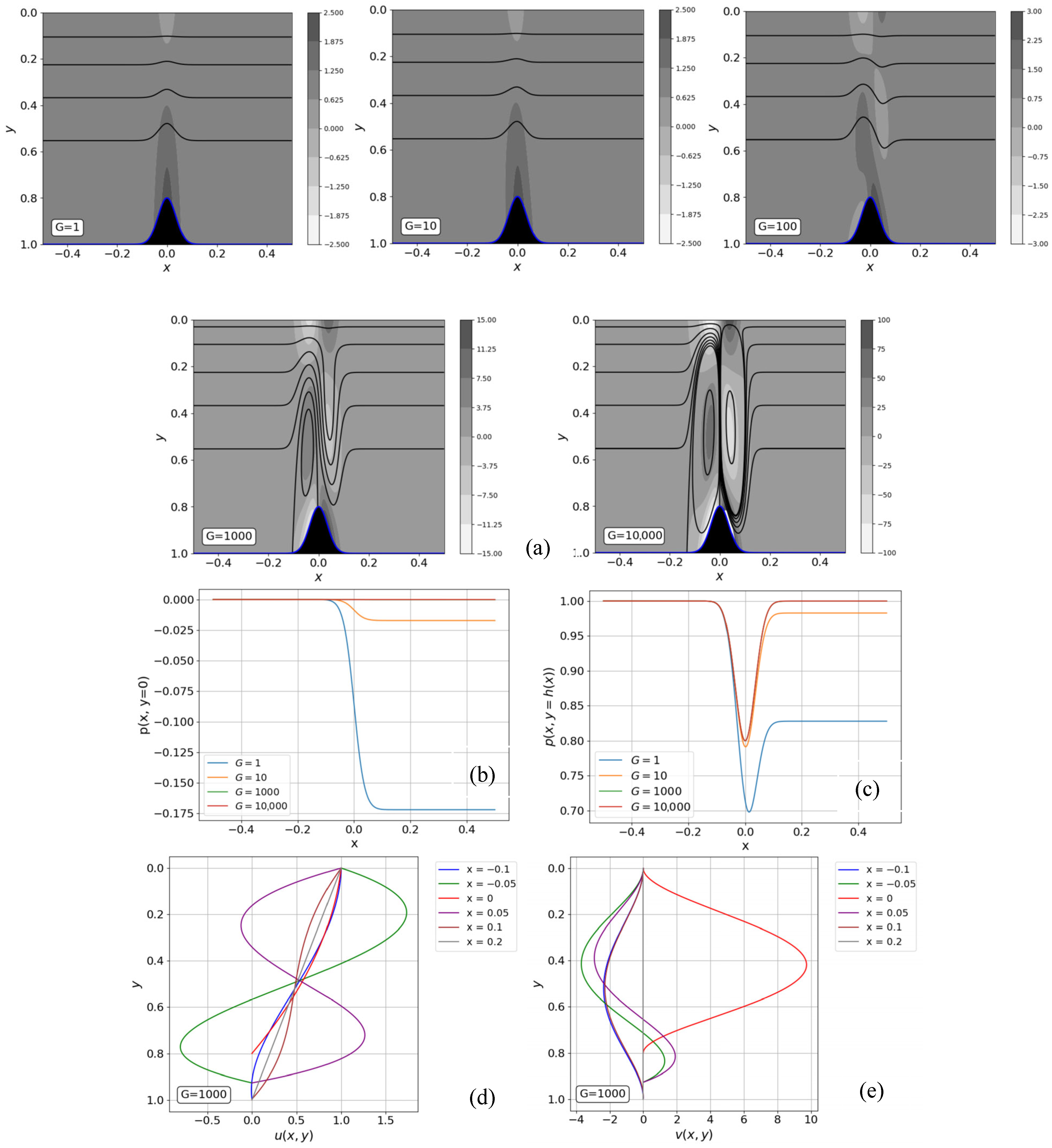
4.2. The Influence of G
We examine the influence of G to investigate the range of flow regimes for fixed moderate density and gravitational stratifications given by r = a = 0.9. The overall influence of G is illustrated in Figure 5, where the flow field and vorticity contours are depicted for 1 < G < 10,000 (Figure 5a). The corresponding pressure distributions along the top and bottom boundaries are also shown in Figure 5b and Figure 5c, respectively, as well as the u and v profiles at different x positions for G = 1000 in Figure 5d,e. It is worth mentioning that the relatively large G value in Figure 5 may appear too large for the narrow-gap approximation to hold. However, we recall that , reflecting the competence between the effects of inertia and gravity. Consequently, the narrow-gap approach should remain valid for large values of G, as long as Re remains moderately small (with Fr being small). Indeed, in our previous work [24], we conducted an extensive comparison between the numerical solution of the Navier–Stokes equation and the narrow-gap results for the zero-gravity gradient. For example, a comparison for an aspect ratio of 0.1 and the cases Re = 1, Fr = 3.2 × 10⁻⁴ (G = 100,000)), Re = 10, Fr = 3.2 × 10⁻³ (G = 1000) and Re = 100, and Fr = 3.2 × 10⁻² (G = 100) led to a very significant agreement in the flow and vortex structure as well as the velocity and pressure fields. Before discussing Figure 4 in detail, the flow may be described for moderately small G and large G ranges. For this, it is helpful to consider the small and large limits of G.
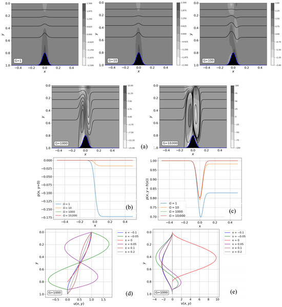
Figure 5.
The influence of G on the flow field for r = a = 0.9. The (a) flow field for 1 < G < 10,000, and the corresponding pressure distributions along the top (b) and bottom (c) boundaries are shown. Also shown are the u (d) and v (e) velocity profiles at different x positions for G =1000 (legends common to both u and v). Here, λ = 0.2 and w = 0.05.
For small G, the velocity in Equation (27) is reduced to the classical profile, with no influence of stratification:
whereas the expressions of the pressure and wall shear stress are reduced to the following:
This shows, in particular, that the pressure gradient is independent of y. More importantly, and as expected, the small G limit obliterates the effects of both the density and gravitation stratifications, even when and . In this case, the flow field remains, as given by Equations (27)–(29). This behavior is typically reflected in Figure 5 for G < 10. In this range, the streamlines are essentially parallel to the bottom topography near the bottom of the plate, gradually becoming horizontal closer to the top of the moving plate. There is a slight loss of symmetry in the flow field for G = O(10) and an increase in the symmetry of the pressure along the bottom topography.
On the other hand, for large values of G, assuming density stratification, the following is obtained :
Clearly, this limit is singular since Equation (43) does not satisfy the condition at the top plate. Both the velocity components and wall shear stress are of O(G). Interestingly, Equation (44) indicates that the pressure remains at O(1). We should, therefore, expect that, as the value of G increases, the flow transitions to a different regime near the top moving plate where the velocity gradient becomes large. In this case, Equation (43) remains valid away from the top plate (in the bulk region of the flow). The boundary-layer characteristic became clearer as we examined the flow by increasing G.
In particular, we assessed the conditions for the onset of vortex motion, which is reflected by the condition for flow separation. In this regard, Equations (39)–(48) for small and large G, as well as the general Equation (30), clearly reflect the role of density and gravity stratification in causing separation and vortex motion. We observe that for G = O(100), the flow field exhibits antisymmetric standing waves across the channel, especially above the obstacle region. For a higher G value, namely when G = O(1000), the standing waves give way to vortex flow upstream of the obstacle, spanning across the channel, accompanied by a significant distortion of the standing wave downstream of the obstacle. The singularity of the velocity predicted in Equation (43) is reflected in Figure 4, where both u and v evolve rapidly near the boundaries.
As outlined below, the vortex flow intensifies both upstream and downstream of the obstacle for more pronounced stratification.
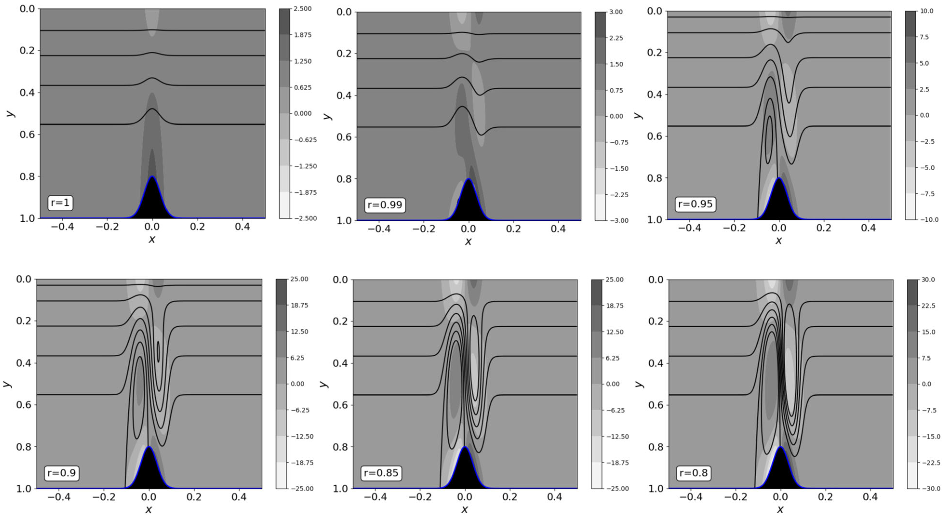
4.3. The Effect of the Density Stratification
The effect of density stratification is assessed by examining the flow for constant gravity (a = 1) and varying the density gradient r for G = 1000. The reduced key expressions are conveniently reproduced here as follows:
Figure 6 illustrates the increasing influence of the density stratification (decreasing r from 1) on the flow field. The sequence in Figure 6 shows that in the absence of a density gradient (r = 1), the flow field is affected by the presence of the obstacle, as suggested by (49) when r = 1. For a small density gradient (r = 0.99), internal antisymmetric gravity waves are visible, which are reminiscent of those observed in the lee of ridges by Sutherland and Aguilar [22] in their experiments. The waves in Figure 6 intensify in amplitude when r = 0.95, resulting in the loss of symmetry and a vortex that forms upstream of the obstacle. For a stronger density gradient (r = 0.9), the vortex is pushed down as a result of the flow distortion near the moving top plate. Simultaneously, a second vortex forms downstream of the obstacle, and a jet of fluid forms between the two vortices, resulting in a blocking flow pattern similar to that described by Long [28,29]. Upon further decreases in r, the figures for r = 0.85 and 0.8 indicate that the vortex structure remains essentially and qualitatively unchanged, but the vortical flow intensifies, as reflected by the tightening of the streamlines.
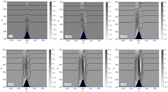
Figure 6.
The influence of density stratification over the range 0.8 ≤ r ≤ 1 in the absence of a gravity gradient (a = 1) on the flow field for G = 1000. Streamlines and vorticity contours are shown. Here, λ = 0.2 and w = 0.05.
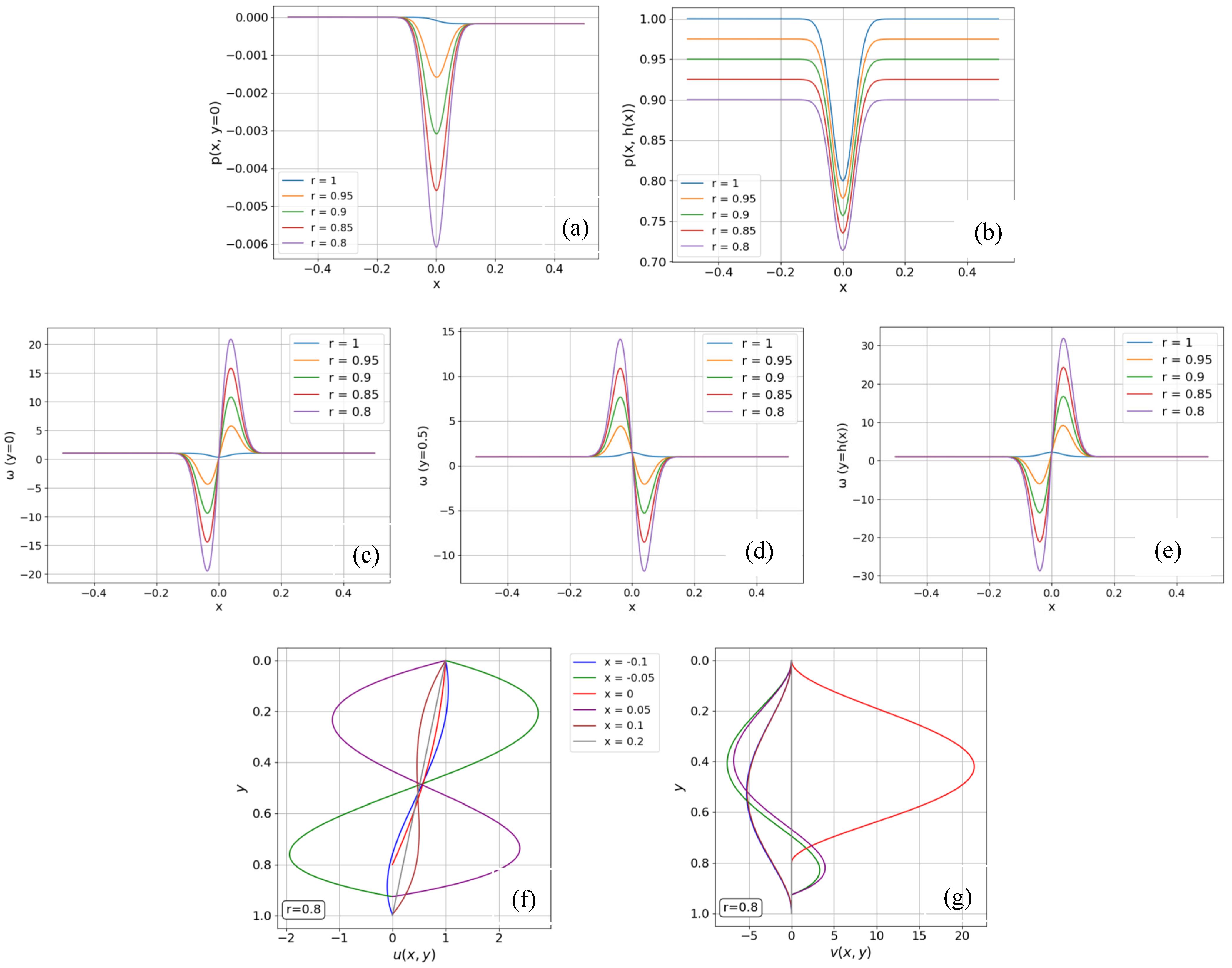
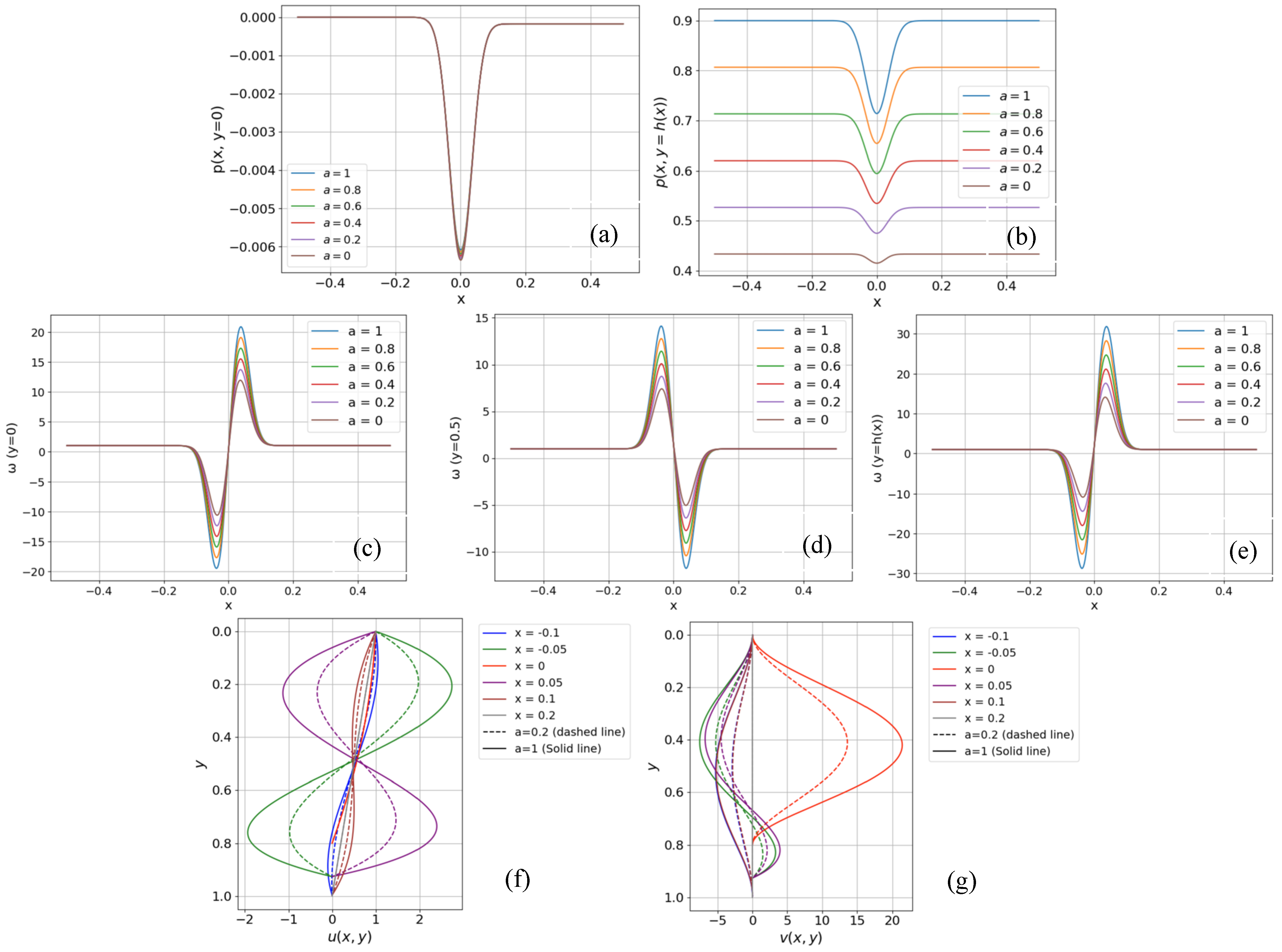
Further details on the flow are shown in Figure 7, namely the distributions of pressure and shear stress along the top and bottom boundaries as well as the velocity distributions for r = 0.8. The behavior of the pressure becomes clearer when inspecting the pressure gradients from Equation (51) along both the top (Figure 7a) and bottom (Figure 7b) boundaries:
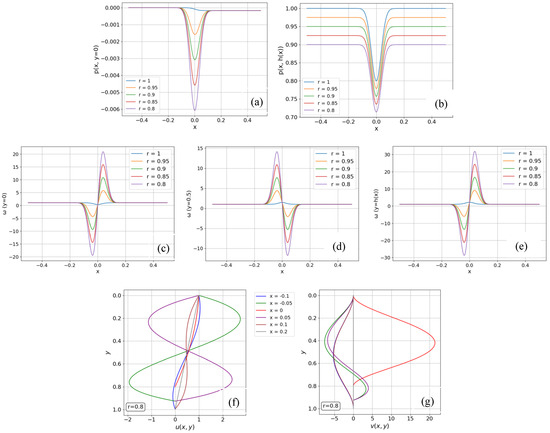
Figure 7.
The influence of density stratification at constant gravity (a = 1) on the flow field over the range 0.8 ≤ r ≤ 1 for G = 1000. The pressure distributions along the top (a) and bottom (b) boundaries are shown alongside the vorticity distributions along the top (c), midway (d), and bottom (e) boundaries. The u (f) and v (g) velocity profiles at different x positions are also shown (legends common to both u and v). Here, λ = 0.2 and w = 0.05.
Clearly, for relatively large G values, the pressure gradient along the two boundaries is dominated by the term proportional to the bottom slope. Figure 7a illustrates how the pressure transitions from a monotonically decreasing function along the top plate for a constant density fluid (r = 1) to a pressure developing a minimum that strengthens with increasing density stratification (r < 1). This change in behavior is also reflected in the pressure gradient at y = 0 from Equation (52). The presence of an adverse pressure gradient at the upper boundary, which is parallel to a streamline in the flow, allows flow separation to occur in a stratified flow, forming the vortices shown in Figure 7c–e. The pressure along the bottom boundary in Figure 7b shows a similar trend except that, for r = 1, the pressure still displays a minimum instead of the monotonically decreasing trend reported in Figure 4. Interestingly, this behavior is exhibited regardless of the G value.
The vorticity or wall shear stress along the top (Figure 7c) and bottom (Figure 7e) boundaries for a = 1 from Equation (30) is reduced to the following:
We can see that the vorticity (shear stress) is negative except along the top wall if either h < ¾ or G is relatively small 1 − r. Vorticity along the boundaries is antisymmetric for a constant-density fluid, and this symmetry is lost as r decreases from one. Symmetry is gradually regained (see the r = 0.8 curves) as the density gradient increases because of the dominance of the G(1 − r) term in Equation (53).
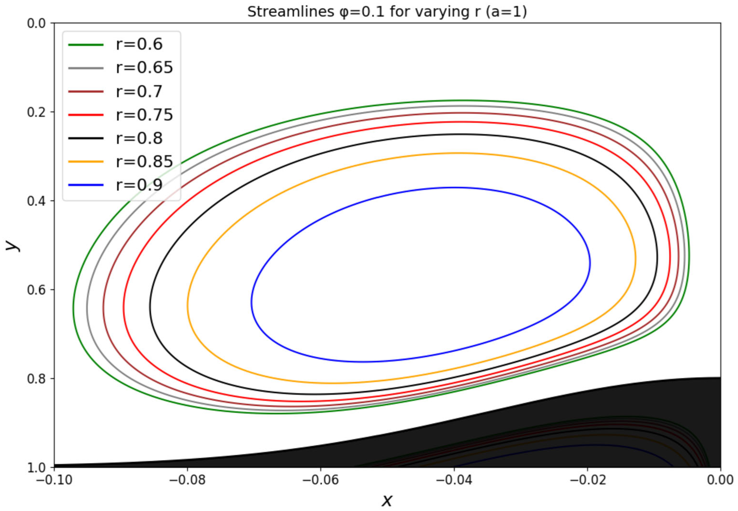
A closer assessment of the influence of density stratification on the vortex structure is depicted in Figure 8, where we plotted the closed central vortex above the left-hand side of the obstacle for different values of . As expected, the size of the vortex grew with density stratification, both in width and height. Given the fluid confinement between two rigid boundaries, the vortex cannot grow indefinitely with increasing density stratification. Indeed, Figure 8 indicates that growth saturation occurs for r < 0.6, when the vortex occupies 70% of the fluid gap in height. The saturation is particularly obvious near the obstacle and the vertical line x = 0. The vortex size is examined further below when we discuss the interplay between the density and gravity stratifications.
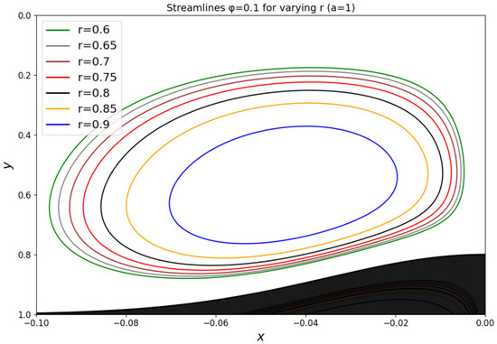
Figure 8.
The influence of density stratification on the vortex shape upstream of the obstacle over the range 0.6 ≤ r ≤ 1 in the absence of a gravity gradient (a = 1) for G = 1000. Here, λ = 0.2 and w = 0.05.
4.4. Interplay Between Density and Gravity Stratifications
Gravity acts on density variation, which is, therefore, required for gravity and its stratification to affect the flow; Equations (27)–(30) confirm that for gravity stratification to significantly manifest itself in the flow, the effect of density stratification cannot be negligible. In fact, on setting r = 1, some interesting observations are worth noting here. The effect of gravity stratification vanishes entirely from Equations (27) and (28) for the velocity components, which is expected because the full Navier–Stokes equations show that, without density variation, gravity only affects the vertical pressure profile and not the velocity field. The velocity field is now independent of any parameter, namely of both G and a, while the deviation from the linear pressure profile is due to the variation in gravity. The velocity profile is parabolic and of the Poiseuille–Couette type, as seen in Equation (32). Consequently, unlike density stratification, gravity stratification alone cannot lead to vortex generation. Gravity stratification remains only influential on the pressure as Equation (29) suggests, which is reduced to the following:
The pressure is parabolic instead of cubic in y, and the gravity gradient (a < 1) diminishes its value everywhere. The streamwise pressure gradient is independent of the height, depending solely on the bottom topography. Simultaneously, the pressure does not exhibit the modulation in x reported earlier in Figure 4 and Figure 5. In fact, since and h < 1, the pressure decreases monotonically regardless of obstacle shape and gravity gradient, as seen in Equation (35).
The interplay between density and gravity stratifications is further assessed in Figure 9 and Figure 10 by examining the flow for a constant density gradient (r = 0.8) and varying the gravity gradient. The impact of gravity variation modulates the effect of stratification on the flow. We discuss the influence of gravity stratification on the flow field by referring to Figure 9, where the streamlines are plotted along with the vorticity contours for r = 0.8 and . The increase in the gravity gradient diminishes the vortex intensity, which is clearly visible when a is decreased from 1 to 0 in Figure 9. For a small gravity variation, the flow tends to compress the upstream vortex and causes the downstream vortex to open from the top, as shown for . Upon the further increase in the gravity gradient, the upstream vortex is further compressed and distorted while the downstream vortex continues to open at the top but with little change at the bottom (0 < a < 0.4). As the gravity gradient increases, gravity becomes weaker toward the bottom of the domain, weakening the overall effect of stratification. This occurs because stratification only affects the flow field in the presence of gravity, so as gravity weakens, the effect of stratification decreases, and the vortices, which only form due to stratification, become smaller and weaker.
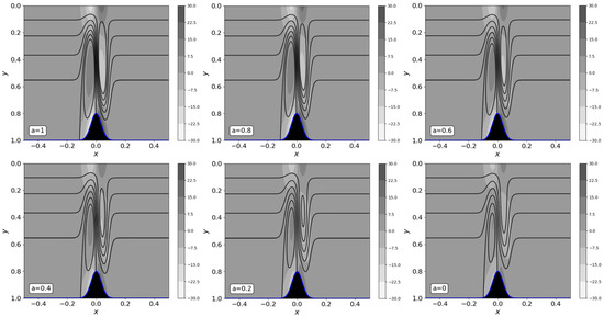
Figure 9.
The influence of gravity stratification in the range 0 ≤ a ≤ 1 in the presence of a density gradient (r = 0.8) in the flow field for G = 1000. Streamlines and vorticity contours are shown. Here, λ = 0.2 and w = 0.05.
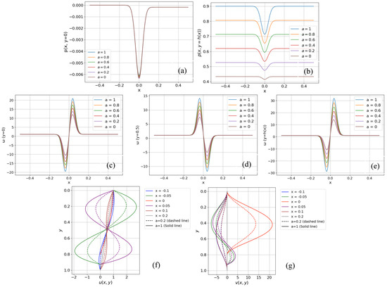
Figure 10.
The influence of gravity stratification at a constant density gradient (r = 0.8) on the flow field in the range 0 ≤ a ≤ 1 for G = 1000. The pressure distributions along the top (a) and bottom (b) boundaries are shown, as well as the vorticity distributions along the top (c), midway (d), and bottom (e) boundaries. Also shown are the u (f) and v (g) velocity profiles at different x positions (legends common to both u and v). Here, λ = 0.2 and w = 0.05.
The relatively small change in qualitative behavior is also reflected rather starkly in Figure 10, where the pressure and vorticity distributions are shown. Recalling Equation (29), the pressure distribution along the boundaries is as follows:
The pressure distributions in Figure 10 indicate that the pressure at the upper boundary (Figure 10a) remains essentially unaffected by the gravity gradient, whereas the pressure at the bottom (Figure 10b) decreases rather significantly as a decreases. This decrease is essentially linear with a as the terms following the integral in Equation (56) suggest. Since G is relatively large, the pressure is essentially given by Equation (44), which shows that the pressure distribution is indeed symmetric everywhere.
This is also reflected in the vorticity from Equation (30) along the top (Figure 10c) and bottom (Figure 10e) boundaries:
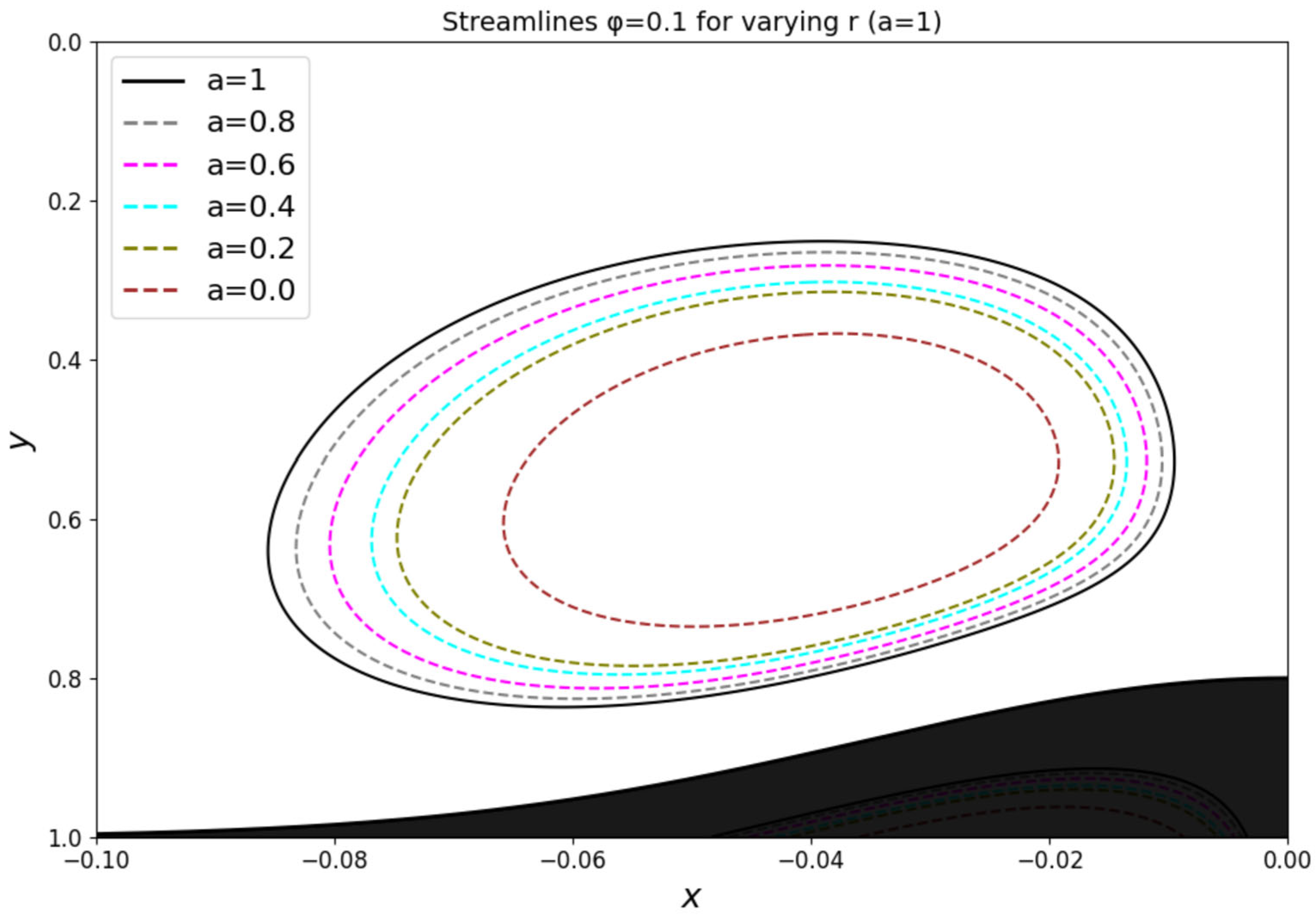
The interplay between density and gravity stratifications was further assessed by examining the effect on the vortex shape and size. Figure 11 depicts the dependence of the vortex shape on gravity stratification in the range for r = 0.8. A strong gravity stratification prohibits vortex formation (the smallest vortex corresponds to a = 0).
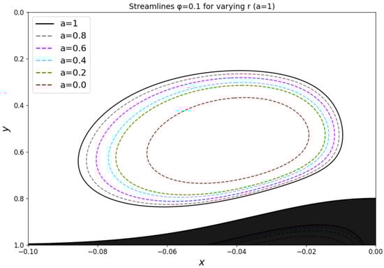
Figure 11.
The influence of gravity stratification on the vortex shape upstream of the obstacle over the range 0 ≤ a ≤ 1 for r = 0.8 and G = 1000. Here, λ = 0.2 and w = 0.05.
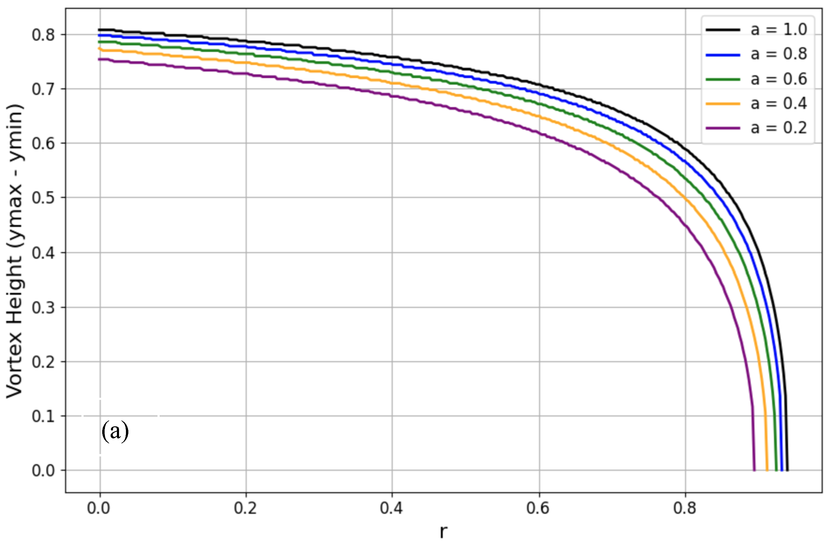
A further quantitative assessment is reported in Figure 12, where the height of the vortex is plotted against r (Figure 12a) and against a (Figure 12b). A three-dimensional perspective is given in Figure 12c. Figure 12a suggests a slow decrease in the vortex size with an increasing value of r, except for r > 0.8, in which range the vortex size decreases sharply as a result of the fluid layer’s confinement between two rigid boundaries. Figure 12b reflects a mild increase in vortex size with a diminishing gravity gradient. This increase is mildest for a heavily density-stratified layer (r = 0). Although the overall vortex height diminishes with density stratification, the growth rate as a increases. Eventually, the vortex height must tend towards zero as . Figure 12b suggests that the vortex tends to shrink with density stratification and disappears completely in the small a range of r > 0.85.


Figure 12.
The influence of density and gravity stratifications on the vortex shape upstream of the obstacle over the ranges (0 ≤ a ≤ 1, 0 ≤ r ≤ 0.85) and G = 1000. The dependence of the vortex size on (a) r for different a and (b) for different r values is shown. A three-dimensional perspective is given in (c). Here, λ = 0.2 and w = 0.05.
The effect of gravity stratification on the vortex structure can also be illustrated by considering instances when gravity increases toward the bottom of the domain and comparing the results to the original case with gravity decreasing toward the bottom of the domain. Corresponding cases with the same vertical integral of gravity, and therefore, the same overall strength of gravity, can be considered by taking and for a case with gravity increasing toward the top and and for a case with gravity increasing toward the bottom. The relevant non-dimensional parameters in the flow are a, r, and G. In the case with decreasing gravity from dimensional values of b to c (c < b) toward the bottom of the domain, as illustrated in Figure 13, , while in the case of increasing gravity from c to b towards the bottom of the domain, In the case of decreasing gravity from the dimensional values of b to c toward the bottom of the domain, while for increasing gravity toward the bottom, , since Re and ε are unchanged from case 1 to case 2.
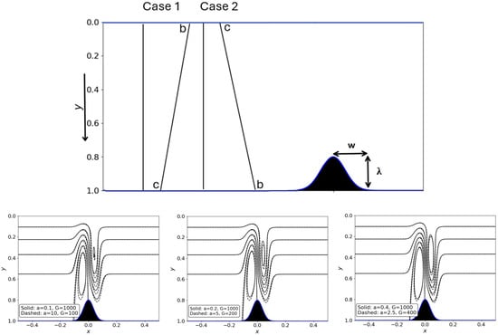
Figure 13.
Dimensional gravity profiles for corresponding cases of decreasing and increasing gravity toward the bottom of the domain, where both cases have an equivalent vertical integral of gravity (top). The streamlines for pairs of corresponding cases with gravity increasing or decreasing toward the bottom of the domain are given.
Streamlines for pairs of corresponding cases with gravity increasing toward the top and bottom show that the vortex shifts toward the direction of stronger gravity, as seen in Figure 13. This occurs due to the vortices resulting from the combined effect of gravity and stratification. For a specified, constant stratification, the vortex is stronger in the region of stronger gravity and weaker in the region of weaker gravity. The shift is small because the topographic bump is essential in generating the vortex, and its position remains the same for both cases. In the case of stronger gravity near the bottom of the domain, where the topography is located, the upstream vortex is larger than in the case of larger gravity near the top of the domain; gravity and topography both contribute to generating the vortices, so when stronger gravity occurs in the vicinity of the bump, the vortex is stronger. The downstream vortex appears to exhibit a shift without a significant change in size.
4.5. Influence of Obstacle Size
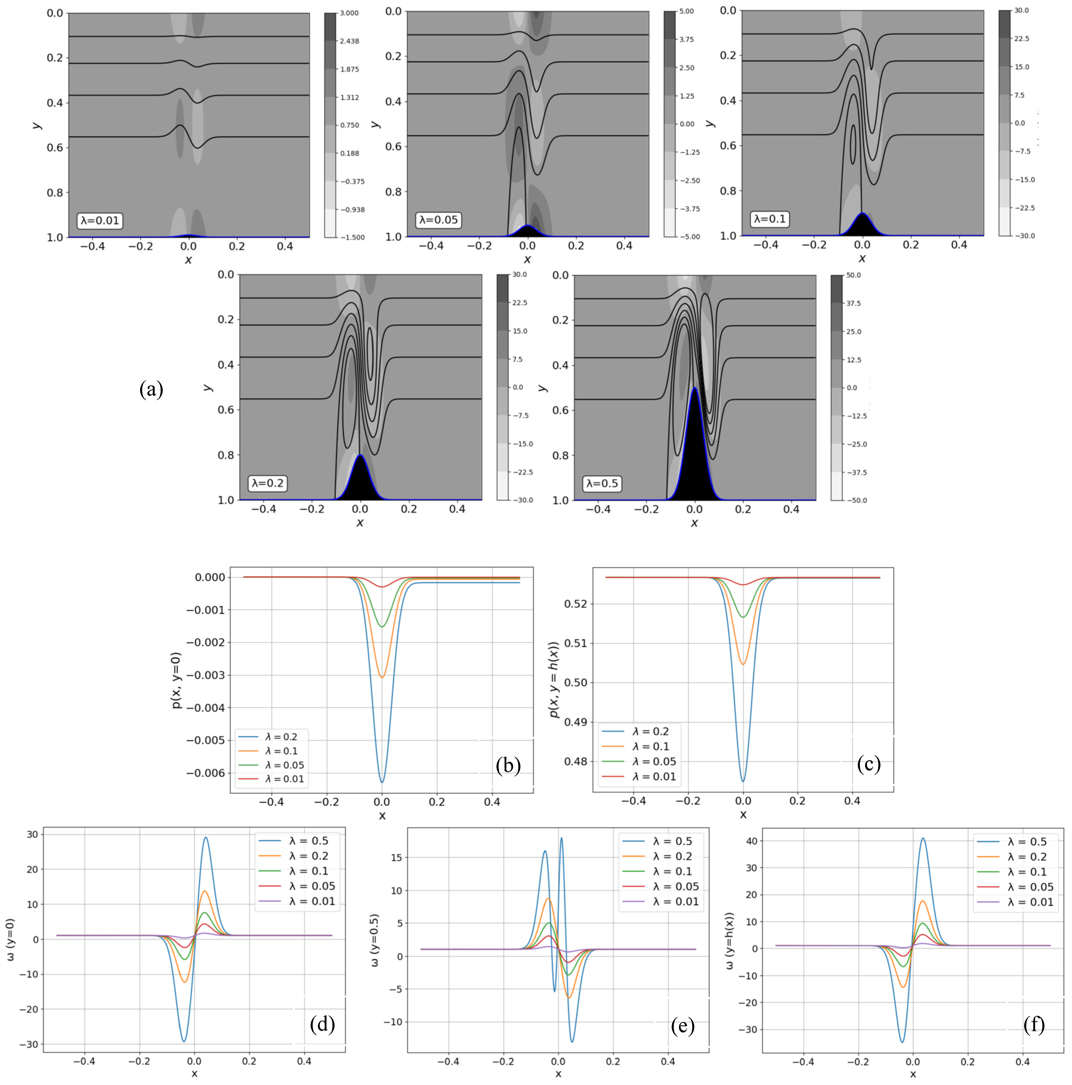
We next consider the influence of the obstacle size on the flow by examining obstacles of various heights and widths. The results correspond to G = 1000, r = 0.8, and a = 0.2. Figure 14 depicts the influence of the obstacle amplitude for a fixed width w = 0.05. We plotted the flow field (Figure 14a), pressure (Figure 14b,c), and vorticity (Figure 14c,e) along the solid boundaries for the range . Even when the amplitude was negligibly small (λ = 0.01), the flow displayed how non-symmetric gravity waves were weakened in amplitude with increasing distance from the obstacle. As the obstacle height increased (λ = 0.05), the wave amplitude increased with additional distortion; a vortex began to emanate upstream of, and close to, the obstacle. For λ = 0.1, the vortex was well established upstream of the obstacle, but the standing waves still persisted downstream, with increased amplitude and distortion. Interestingly, despite the strong dissymmetry in the flow field, which was also exhibited by vorticity, the pressure remained symmetric for all obstacle amplitudes considered (Figure 14), which seemed to be controlled by the large G value. As the obstacle height increased further, a vortex appeared downstream of the obstacle for λ = 0.2, and became well established by λ = 0.5. Simultaneously, both the pressure and vorticity intensified in magnitude with no qualitative change.
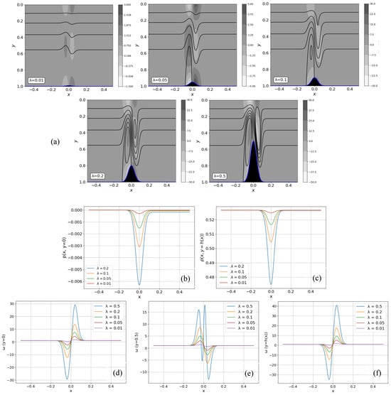
Figure 14.
The influence of the obstacle height on the flow field over the range 0.01 ≤ λ ≤ 0.2 in the presence of density and gravity gradients (r = 0.8, a = 0.2) for G = 1000. The streamlines and vorticity contours (a), as well as the pressure distributions along the top (b) and bottom (c) boundaries, and the vorticity distributions along the top (d), midway (e), and bottom (f) boundaries are shown. The obstacle width is fixed at w = 0.5.
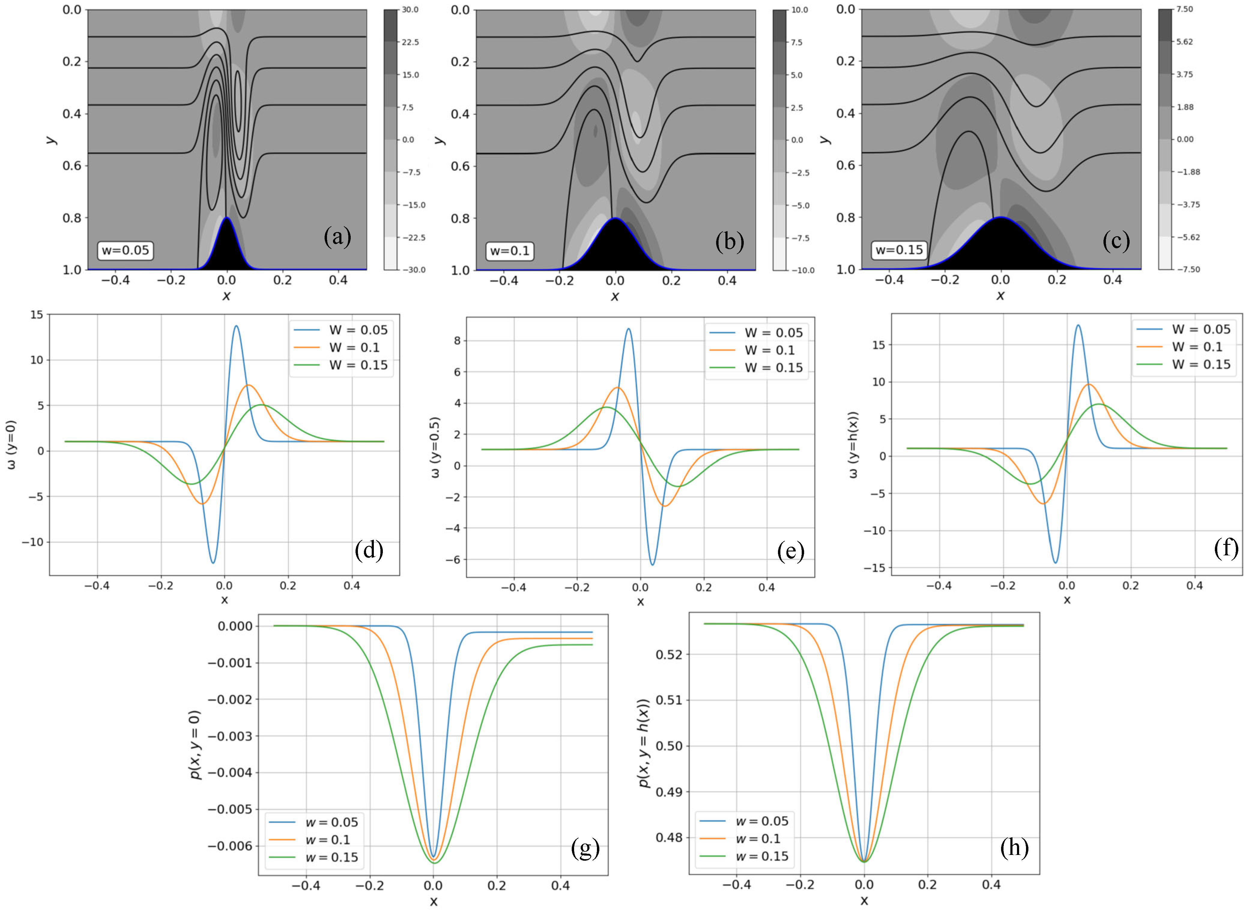
Finally, we consider the impact of the obstacle width on the flow for a fixed obstacle amplitude (λ = 0.2) and variable width (0.05 < w < 0.15) as shown in Figure 15. The flow for w = 0.05 in Figure 15a corresponds to the last case examined in Figure 14a (λ = 0.5, w = 0.05), depicting well-established vortices both upstream and downstream of the obstacle. For a larger obstacle width (w = 0.1), Figure 15b suggests that both vortices are distorted, spanning the obstacle width. The upstream vortex widens, and the downstream vortex disappears, giving way to standing waves, suggesting that the presence of the downstream vortex is dependent on the slope of the topography, as well as the topographic height and stratification. For an even wider obstacle (w = 0.15), Figure 15c shows only standing waves prevailing over the obstacle region. Interestingly, both the vorticity (Figure 15d–f) and pressure (Figure 15g,h) along the boundaries retained the same magnitude independently of the obstacle width.
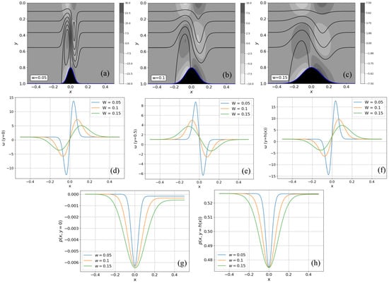
Figure 15.
The influence of the obstacle width on the flow field over the range 0.05 ≤ w ≤ 0.15 in the presence of density and gravity gradients (r = 0.8, a = 0.2) for G = 1000. The streamlines and vorticity contours (a–c), and the vorticity distributions along the top (d), midway (e), and bottom (f) boundaries, as well as the pressure distributions along the top (g) and bottom (h) boundaries, are shown. The obstacle height is fixed at λ = 0.5.
5. Discussion and Conclusions
In the absence of gravity stratification for reference, a wider range of realistic physical parameters, and additional details on the complex vortex structure were included. Thus, while the setup may appear structurally similar, the governing physical mechanisms are fundamentally altered through the addition of a varying gravitational field, which is a modification that has profound implications on the flow behavior. This forms a critical and realistic extension with important physical and interdisciplinary implications. Since gravity is a volume force, it can easily represent other volume forces, such as varying magnetic and electric fields for a stratified conducting fluid, widening the range of fundamental investigations using the current formulation.
This narrow-gap approach is used to study the effects of gravity variation on a density-stratified flow over topography in a channel, driven by the motion of the upper plate. Without stratification, the flow passes smoothly over the topography. While an adverse pressure gradient develops along streamlines close to the topography, the velocity profile shows that flow separation does not occur. For a weak density-stratified fluid, the streamlines become distorted, forming standing gravity waves. As the strength of stratification increases, separation occurs, and vortices appear upstream and downstream of the obstacle. The effects of stratification strength, gravity variation, the magnitude of topographic height, and topography width are investigated, and two factors are ultimately found to affect the strength of the vortices: the coupling of gravity and stratification, and the slope of the topography, described by the aspect ratio ε.
Stratification is found to be a necessary condition for vortex generation in the region of topographic variation, and stronger stratification results in stronger vortices. The effect of density stratification is negligible without the influence of gravity, and therefore, the two effects are coupled. Similarly, gravity only affects the velocity field in the presence of density variation. Gravity variation is introduced as a reduction in the strength of gravity toward the bottom of the domain, and as the overall strength of gravity decreases, the coupled effect of stratification and gravity decreases. Therefore, the strength of the vortices also decreases when gravity variation is introduced.
The other effect contributing to vortex strength is the topographic slope; a steeper topography, presenting as either a taller or narrower bump, increases the vortex strength. A higher magnitude of the non-dimensional grouping also results in stronger vortices. The parameter incorporates both of the aforementioned effects; a larger G value may result from stronger gravity relative to the inertia of the flow or a larger ε, which corresponds to a higher aspect ratio topography, with steeper sides.
Finally, while this study is obviously of a fundamental nature, it has widespread relevance to applications. As we mentioned in the introduction, in most natural and astrophysical settings, gravity is rarely uniform. From the Earth’s core to stellar interiors, the gravitational field typically varies with position, especially in the vertical direction due to self-gravitating effects. The current study uniquely models this by introducing a varying gravity field into the governing equation, boundary conditions, and solution, and explores its interaction with density stratification. This represents a new area in baroclinic flow analysis. The classical vortex and internal wave structures in stratified flows are shown to be significantly modified when gravity varies with height, which is an insight not available in the existing literature. Vortices may shift, stretch, or weaken depending on the direction and strength of gravity variation, and internal waves develop asymmetries or damping that were not present under constant gravity. The current study potentially extends beyond traditional fluid dynamics. Gravity gradients are common in planetary interiors, stellar atmospheres, and black hole accretion flows; the insight offered here is directly relevant to astrophysicists and geophysicists when observing flow patterns under variable gravitational fields. Such a coupling of gravitational physics with baroclinic fluid behavior allows the potential inference of gravitational structures from observable flow fields, offering an indirect diagnostic tool in celestial modeling.
Author Contributions
K.S.G.: Conceptualization (equal); Data curation (equal); Formal analysis (equal); Methodology (equal). R.E.K.: Conceptualization (equal). K.A.O.: Conceptualization (equal). All authors have read and agreed to the published version of the manuscript.
Funding
The financial support of the Natural Sciences and Engineering Research Council of Canada (NSERC) is gratefully acknowledged.
Data Availability Statement
The data that support the findings of this study are available from the corresponding author upon reasonable request.
Conflicts of Interest
The authors have no conflicts of interest to disclose.
References
- Bigg, E. Atmospheric stratification revealed by twilight scattering. Tellus 1964, 16, 76–83. [Google Scholar] [CrossRef]
- MacIntyre, S.; Alldredge, A.L.; Gotschalk, C.C. Accumulation of marine snow at density discontinuities in the water column. Limnol. Oceanogr. 1995, 40, 449–468. [Google Scholar] [CrossRef]
- Turner, J.S.; Campbell, I. Convection and mixing in magma chambers. Earth-Sci. Rev. 1986, 23, 255–352. [Google Scholar] [CrossRef]
- Balbus, S.A.; Soker, N. Resonant excitation of internal gravity waves in cluster cooling flows. Astrophys. J. 1990, 357, 353–366. [Google Scholar] [CrossRef]
- Li, T.; Wan, M.; Chen, S. Evolution of a stratified turbulent cloud under rotation. Atmosphere 2023, 14, 1590. [Google Scholar] [CrossRef]
- More, R.; Balasubramanian, S. Mixing dynamics in double-diffusive convective stratified fluid layers. Curr. Sci. 2018, 114, 1953–1960. [Google Scholar] [CrossRef]
- Dziewonski, A.M.; Anderson, D.L. Preliminary reference Earth model. Phys. Earth Planet. Inter. 1981, 25, 297–356. [Google Scholar] [CrossRef]
- Stevenson, D.J. Planetary magnetic fields: Achievements and prospects. Earth Planet. Sci. Lett. 2003, 208, 1–11. [Google Scholar]
- Turcotte, D.L.; Schubert, G. Geodynamics, 3rd ed.; Cambridge University Press: Cambridge, UK, 2014. [Google Scholar]
- Butcher, H. Fundamental principles for static sealing with metal in high pressure field. ASME Trans. 1973, 16, 304. [Google Scholar]
- Matthias, S.; Müller, F. Asymmetric pores in a silicon membrane acting as massively parallel Brownian ratchets. Nature 2003, 424, 53–57. [Google Scholar] [CrossRef] [PubMed]
- Stone, H.A.; Stroock, A.D.; Adjari, A. Slippage of liquids over lyophobic solid surfaces. Annu. Rev. Fluid Mech. 2004, 36, 381–411. [Google Scholar] [CrossRef]
- Long, R.R. Some aspects of the flow of stratified fluids: III. Continuous density gradients. Tellus 1955, 7, 341–357. [Google Scholar] [CrossRef]
- Langlois, W.E. Slow Viscous Flow; Macmillan: New York, NY, USA, 1964. [Google Scholar]
- Leal, L.G. Advanced Transport Phenomena: Fluid Mechanics and Convective Transport Processes; Cambridge University Press: Cambridge, UK, 2007. [Google Scholar]
- Ockendon, H.; Ockendon, J.R. Viscous Flow; Cambridge University Press: Cambridge, UK, 1995. [Google Scholar]
- Tavakol, B.; Froehlicher, G.; Holmes, D.P.; Stone, H.A. Extended lubrication theory: Improved estimates of flow in channels with variable geometry. Proc. R. Soc. A 2017, 473, 20170234. [Google Scholar] [CrossRef] [PubMed]
- Housiadas, K.D.; Tsangaris, C. High-order lubrication theory in channels and tubes with variable geometry. Acta Mech. 2022, 233, 4063–4081. [Google Scholar] [CrossRef]
- Luberto, L.; de Payrebrune, K.M. Examination of laminar Couette flow with obstacles by a low-cost particle image velocimetry setup. Phys. Fluids 2021, 33, 033603. [Google Scholar] [CrossRef]
- Yih, C.-S. Exact solutions for steady two-dimensional flow of a stratified fluid. J. Fluid Mech. 1960, 9, 161–174. [Google Scholar] [CrossRef]
- Claus, A. Large-amplitude motion of a compressible fluid in the atmosphere. J. Fluid Mech. 1964, 19, 267–289. [Google Scholar] [CrossRef]
- Sutherland, B.R.; Aguilar, D.A. Stratified flow over topography: Wave generation and boundary layer separation. WIT Trans. Eng. Sci. 2006, 52, 10–20. [Google Scholar] [CrossRef]
- Zaza, D.; Iovieno, M. Influence of coherent vortex rolls on particle dynamics in unstably stratified turbulent channel flows. Energies 2024, 17, 2725. [Google Scholar] [CrossRef]
- Wang, W.; Khayat, R.E. Stratification-induced vortex flow in a channel with topography. Eur. Phys. J. Spec. Top. 2024, 233, 1573–1587. [Google Scholar] [CrossRef]
- Halliday, D.; Resnick, R.; Walker, J. Fundamentals of Physics, 7th ed.; John Wiley & Sons: Hoboken, NJ, USA, 2005; p. 335. [Google Scholar]
- Gao, X.; Liu, Z.; Tian, X.; Chen, Y. Numerical investigation of internal interface behavior in two-layer stratified flow. J. Hydraul. Res. 2024, 62, 74–85. [Google Scholar]
- Schlichting, H.; Gersten, K. Grenzschicht-Theorie, 10th ed.; Springer: Berlin/Heidelberg, Germany, 2006. [Google Scholar]
- Long, R.R. The motion of fluids with density stratification. J. Geophys. Res. 1959, 64, 2151–2163. [Google Scholar] [CrossRef]
- Long, R.R. Blocking effects in flow over obstacles. Tellus 1970, 22, 471–480. [Google Scholar] [CrossRef]
Disclaimer/Publisher’s Note: The statements, opinions and data contained in all publications are solely those of the individual author(s) and contributor(s) and not of MDPI and/or the editor(s). MDPI and/or the editor(s) disclaim responsibility for any injury to people or property resulting from any ideas, methods, instructions or products referred to in the content. |
© 2025 by the authors. Licensee MDPI, Basel, Switzerland. This article is an open access article distributed under the terms and conditions of the Creative Commons Attribution (CC BY) license (https://creativecommons.org/licenses/by/4.0/).