Abstract
An in-depth analysis of the two-phase flow in a hydraulic braking pipeline can reveal its evolution process pertinent for designing and maintaining the hydraulic system. In this study, a high-speed camera examined the two-phase flow pattern and bubble characteristics in a hydraulic braking pipeline. Bubble flow pattern recognition, bubble segmentation, and bubble tracking were performed to analyze the bubble movement, including its behavior, distribution, velocity, and acceleration. The results indicate that the gas–liquid two-phase flow patterns in the hydraulic braking pipeline include bubbly, slug, plug, annular, and transient flows. Experiments reveal that bubbly flow is the most frequent, followed by slug, plug, and transient flows. However, plug and transient flows are unstable, while annular flow occurs at a wheel speed of 200 r/min. Bubbles predominantly appear in the upper section of the pipeline. Furthermore, large bubbles travel faster than small bubbles, whereas slug flow bubbles exhibit higher velocities than those in plug or transient flows.
1. Introduction
The gas–liquid two-phase state of the transmission fluid in a pipeline can lead to cavitation, noise, vibration, and deterioration of the pressure transmission characteristics, which quickly reduces the system’s stability and reliability [1]. So far, the investigations into the causes of the gas formation in a transmission fluid focus on aspects such as the dissolved or entering air, absorbed water, induced heat, and alternating transfer pressure. The dissolved or entering air in the brake fluid includes inherent or self-dissolved air in the brake fluid, residual air in the pipeline when the brake fluid is added, and air sucked from the liquid storage tank during braking. Most of the air exists in free or dissolved states. Therefore, they easily form bubbles under the influence of ambient conditions [2]. Moreover, brake fluid is easy to absorb water and turns into vapor under heat and alternating transfer pressure effects. For example, Hunter et al. [3] studied the water absorption of DOT3 brake fluid at the boiling point of 200~250 °C. The study revealed that after six months, one year, and two years, the water content in the brake fluid was 1.5%, 3.0%, and 4.5~5.0%, respectively.
High ambient temperature, the compression effect of the alternating braking pressure, heat dissipation from the engine and car body, and the heat from the brake friction all contribute to an increase in brake fluid temperature. That is, the braking process of a car generates a large amount of heat, which increases the brake fluid temperature. Jun et al. [4] investigated the heating process of a brake system during a high-mountain car test and found that the brake disc temperature and fluid temperature were 526 °C and 163 °C, respectively, after 47 min of continuous braking, leading to vaporization of the water in the brake fluid. Furthermore, the braking frequency of a braking system is several times per second. Acoustic cavitation occurs once the local pressure is lower than the saturated vapor pressure of water [5,6].
The investigation of gas–liquid two-phase flow in a pipeline is of paramount importance, including flow pattern, split-phase holdup, velocity, etc. [7,8]. Many researchers have used the visualization method to study the flow pattern and split-phase holdup because it is noninvasive and has high accuracy. Deng et al. [9] used a high-speed camera to investigate the flow pattern of kerosene (RP-3) in vertical and horizontal quartz tubes at subcritical and supercritical conditions. They observed different flow patterns that are were related to pressure and temperature. Also, Thaker and Banerjee [10] used a high-speed camera to study the flow pattern characteristics of slug and plug flow. They established a relationship between the apparent velocity of gas–liquid two-phase flow and flow pattern parameters such as two flow pattern frequencies (the number of flow patterns passed in a unit of time), flow pattern transformation speed, and length of the liquid-phase and gas-phase parts of the two flow patterns. Considering the large errors in the frequency prediction of slug flow, Al-Safran et al. [11] proposed a probability model that was a function of pipe diameter, liquid phase apparent velocity, and slip factor to predict slug flow frequency. Setyawan et al. [12] examined the influence of fluid characteristics on the wave velocity and frequency of annular flow in a circular tube and indicated that the frequency of the wave decreased with increased viscosity and decreased surface tension of the liquid. In a different research, Al-Kayiem et al. [13] used a high-speed camera to study the characteristics of a slug flow of water and air in a pipeline. Kajero et al. [14] evaluated the effect of viscosity on the flow pattern and bubble behavior of silicone oil in a small-diameter bubble column using electrical capacitance tomography and high-speed photography. They found that the developing slugs in liquid viscosities of 5 and 100 mPa·s were deformed. The Taylor bubble obtained from 1000 mPa·s was called as a prolate spheroid, while that obtained from 5000 mPa·s was called as an oblate spheroid. The bubble behavior was further characterized using the inverse dimensionless viscosity and Eötvös number.
The study of split-phase holdup based on the visualization method is mainly to calculate the volume of the bubbles in a two-phase flow [15]. Therefore, several studies have investigated the calculation method of bubble volume. Pedro et al. [16] used the fuzzy inference to segment images and adjusted the parameters according to the acquisition focus. They used a random Hough transform combined with a neural network to reconstruct the shape of each bubble and calculated its volume to analyze the porosity of the two-phase flow in a pipeline. Ashish and collaborators [17] also proposed a multi-level image analysis method. The bubble was assumed to be an ellipsoid. Whereas the image was used to determine the center, size, and shape of the bubble, the sphere and ellipsoid volume formulae were used to calculate the bubble volume. Lau and co-workers [18] used the watershed algorithm to segment the bubble cluster in an image and calculated the equivalent diameter using the pixel area of each isolated bubble to determine the bubble volume. Moreover, Markus et al. [19] suggested an overlapping object recognition (OOR) algorithm for bubble segmentation. The OOR algorithm was utilized to calculate the overall perimeter of a segment, found the points at the perimeter representing the connecting points of overlapping objects, clustered the perimeter arcs that belonged to the same object, and fitted ellipses on the clustered arcs of the perimeter.
To the best of the author’s knowledge, studies on the gas–liquid two-phase flow pattern identification and bubble characteristics in automobile hydraulic brake pipelines are scarce, especially research involving the visualization method. In light of this importance, this study used the visualization method and image processing technology to comprehensively investigate the gas–liquid two-phase flow in an automobile hydraulic braking pipeline. The novel contribution lies in the system-level integration of bubble-volume-resolved algorithms and their application to the hydraulic-braking context. The paper consists of five parts. In addition to the introduction, Section 2 introduces the experimental device and processes and provides the flow pattern recognition method, bubble volume calculation method, and bubble tracking method. The flow pattern, bubble volume, and bubble velocity are statistically analyzed in Section 3. Section 4 presents the bubble distribution and force situation, and the gas holdup in the selected windows. Finally, Section 5 provides the conclusions of the study.
2. Experimental Device and Research Methods
2.1. Experimental Device
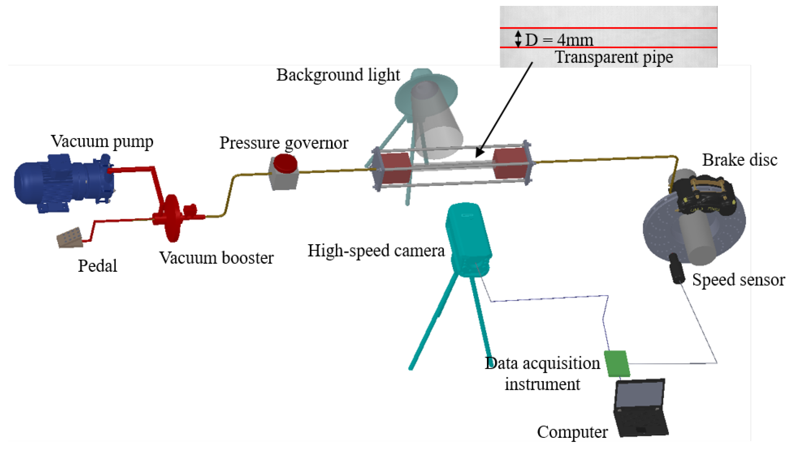
The experimental device is shown in Figure 1. It is a modified Santana 3000 ABS (Anti-braking system, Wanxiang Qianchao Co., Ltd.; Hangzhou, China) test rig, which mainly consists of a hydraulic brake system and a video acquisition module. The hydraulic brake system can control the wheel speed between 0–1600 r/min. A horizontally placed transparent quartz tube with an inner diameter and length of 4 mm and 150 mm, respectively, was installed in the hydraulic pipeline of the right front wheel of the brake platform. The transparent pipeline was equipped with a pressure sensor (Swiss Keller brand PA-25TAB, Beijing Handarsen Machinery Technology Co., Ltd.; Beijing, China) at the ends to measure the pipeline inlet and outlet pressures. The power supply for the pressure sensor was provided by a WD-5 regulated power supply. The pressure sensor used a 15 V power supply with a sampling frequency of 1 kHz. An OLYMPUS·ISPEED·2·MONO (4G) high-speed camera (Olympus Corporation; Tokyo, Janpan) with a resolution of 800 × 600 and a maximum frame rate of 3000 fps was used to record the two-phase flow in the transparent quartz tube. The frame rate used in this study was 100 fps. The BL series (Fuzhou Boring Imaging Equipment Co., Ltd.; Fuzhou, China) studio light was used as backlighting and a sheet of sulfuric acid paper was layered behind the quartz tube to improve the photograph’s quality.
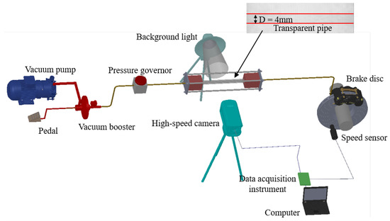
Figure 1.
Experimental facility.
The two-phase flow video was recorded as a sample video at every 100 r/min wheel speed between 200 and 1200 r/min wheel speeds.
2.2. Image Preprocessing
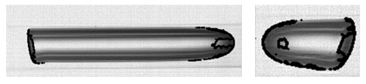
Image processing was performed on the recorded video in the hydraulic braking pipeline using the Python-OpenCV package (3.13.5). The Hough line transformation [20,21] was used to fit the upper and lower boundaries of the transparent pipeline in the video. The pipeline position was corrected by the fitted upper and lower boundary lines to eliminate the small angle between the pipeline and the horizontal direction. According to the inner diameter d of the transparent pipe in the video and the actual inner diameter D of the transparent pipe, the unit length of each pixel grid could be determined as D/d mm. The segmentation of the bubble foreground and pipe background is the premise of bubble contour and bubble feature extraction. Usually, dynamic detection algorithms such as the frame difference [22], background subtraction [23] and vibe [24] are used to complete the image segmentation. However, as shown in Figure 2, it is difficult to identify the bubble contour completely for bubbles with extremely slow movement velocity or uniform intensity of internal pixels using the dynamic detection algorithm.

Figure 2.
Dynamic detection result.
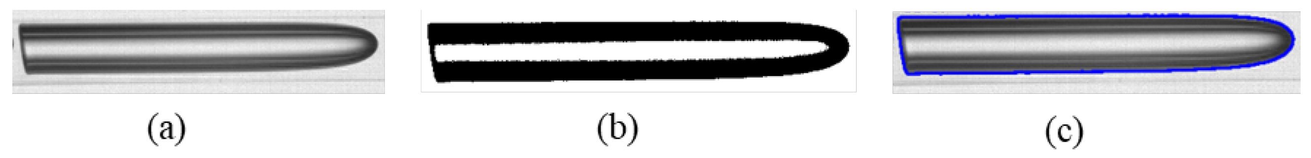
Based on the fitting of the upper and lower boundaries of the pipeline through the Hough transform, the bubble contour was extracted by performing the following steps: (1) The image was masked according to the upper and lower boundaries of the pipeline; (2) An appropriate threshold was selected for Otsu’s binarization of the image, and (3) Contour detection was performed for the image after binarization. The bubble foreground and background were distinguished by binarization. By contour detection, the bubble shape and position were obtained. Figure 3 shows the final contour extraction result.
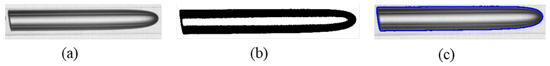
Figure 3.
Extraction. (a) Original image; (b) binarization picture; (c) image after contour detection.
2.3. Bubble Flow Pattern Recognition
2.3.1. Classification of Bubble Flow Pattern
According to the classification method of Ref. [25], the flow patterns in the hydraulic braking pipeline are bubbly, slug, plug, and annular flows (see Figure 4). The bubbles in a bubbly flow are characterized by small volume, large roundness, and a large aspect ratio. The bubbles in the plug flow have a large volume and a good symmetry degree. The bubbles in the slug flow are similar to a bullet shape, with left and right asymmetry. The annular flow bubble is characterized by the air inside the pipeline forming a liquid film on the inner surface of the pipeline. Also, there were bubbles in the pipeline whose shapes were in between the plug flow and slug flow bubbles, as shown in Figure 4e. These bubbles are classified as transient flow bubbles in this paper.
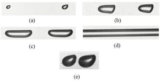
Figure 4.
Image of bubble flow patterns. (a) Bubbly flow bubble; (b) slug flow bubble; (c) plug flow bubble; (d) annular flow bubble; (e) transient flow bubble.
2.3.2. Bubble Classification Criteria
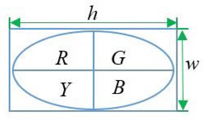
According to the characteristics of each bubble flow pattern described in Section 2.3.1, five bubble shape characteristics, namely area (S), aspect ratio (Ar), roundness (C), area symmetry (SS), and half-area symmetry (HSS), were used as the bubble classification criteria. As Figure 5 shows, the ellipse in the bubble diagram represents the bubble contour and the rectangle on the ellipse is the circumscribed rectangle of the bubble contour, with length and width of h and w, respectively. The two lines in the rectangle divide the circumscribed rectangle equally into four parts. The bubble contour is also divided into four parts by the two lines, with areas R, Y, G, and B. The area S refers to the outline area of the bubble, whereas L is the bubble circumference. The aspect ratio (Ar) is defined as the ratio of the longitudinal length of the bubble to the transverse length of the bubble, which can be obtained from the ratio of the width to the length of the circumscribed rectangle of the bubble (Ar = w/h). The roundness (C) represents the roundness of the bubble. It is calculated as
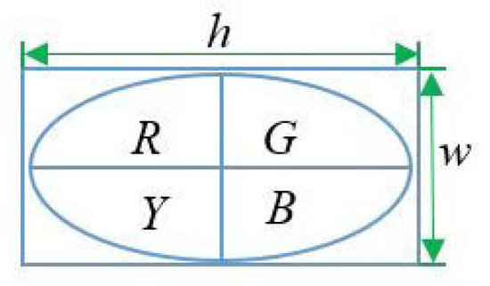
Figure 5.
Bubble diagram.
The ratio of the area in the left and right halves of the bubble is expressed as area symmetry . The ratio of the left and right halves of the upper bubble is expressed as half-area symmetry .
2.3.3. Determination of Classification Characteristics
To find the classification rules for the classification characteristics for each bubble flow pattern, the classification characteristics were extracted from the sample video as the dataset for further analysis. Sometimes, there were bubbles of various bubble flow patterns in the vision window. Herein, the ROI (Region of Interest) man–machine interaction was used to extract the classification characteristics of bubbles in each bubble flow pattern.
As shown in Figure 6, the ROI interaction directly acts on the image after the binarization, so that the bubbles could be better boxed. The largest bubble contour in the box would be displayed. The classification features of the bubble contour are further extracted and labeled with the corresponding bubble flow pattern after confirmation.
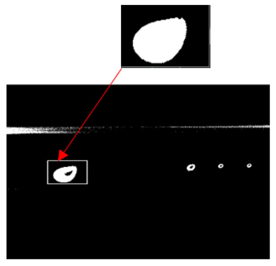
Figure 6.
ROI interaction.
This study obtained a dataset composed of 98 sample data points based on the sample video and further proposed 12 sample data points for each bubble flow pattern from the dataset to form a training set, while the 50 sample data points remained as a test set.
2.3.4. Visualization of Classification Characteristics
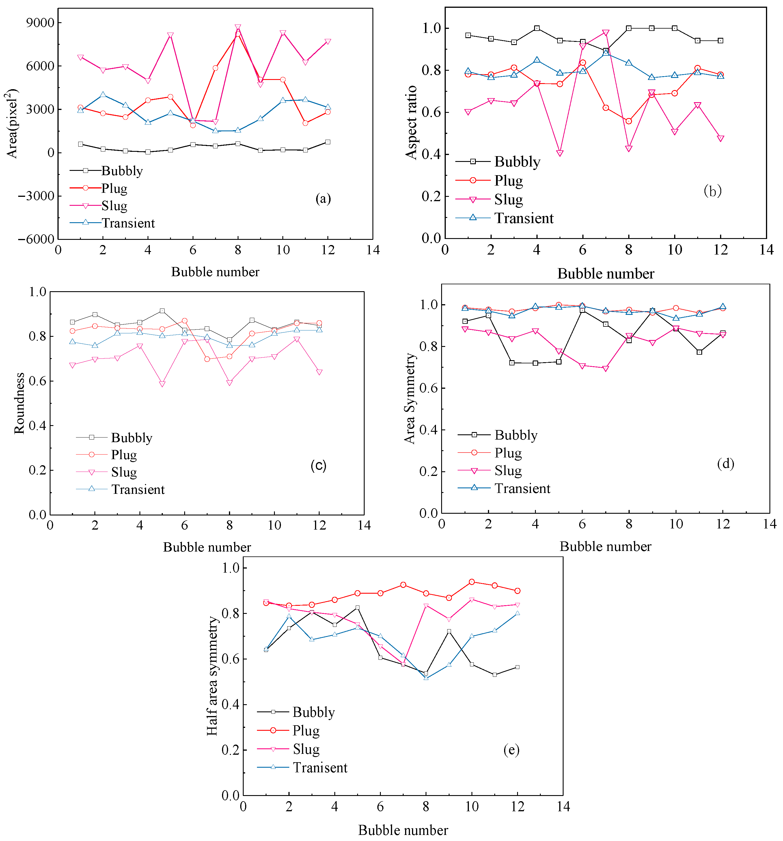
The classification characteristics of each bubble flow pattern in the training set are shown in Figure 7. The figure presents the discrimination effect of different classification characteristics on each bubble flow pattern. The annular flow bubbles have obvious characteristics, which can be distinguished from bubbles of other bubble flow patterns by the aspect ratio and area characteristics, so they are not described in the figure.
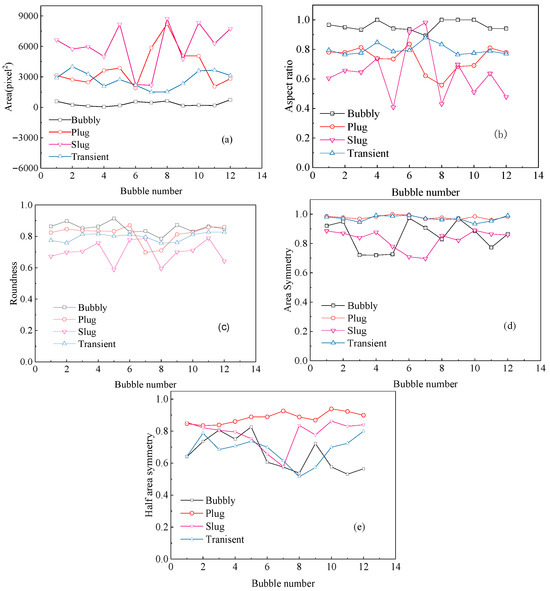
Figure 7.
Classification characteristics of each flow pattern. (a) Area; (b) aspect ratio; (c) roundness; (d) area symmetry; (e) half area symmetry.
Figure 7a shows that the area can distinguish bubbles in bubbly flow from bubbles in the other flow patterns, whereas Figure 7b indicates the aspect ratio of bubbly flow bubbles is generally close to 1. According to Figure 7c, bubbles in bubbly flow and small plug flow exhibit greater roundness, whereas those in transient and slug flow are less round. This classification characteristic plays an auxiliary role in the identification of bubbly and slug flow bubbles. As shown in Figure 7d, plug flow bubbles have greater area symmetry. Furthermore, one side of the slug bubble is sharp as a bullet while the other side is cylinder-like leading to less area symmetry of slug flow bubbles. Transient flow bubbles are asymmetrical in shape but can have symmetrical areas. Therefore, the area symmetry can be used to distinguish plug flow bubbles from slug flow bubbles. Referring to Figure 7e, the half-area symmetry can be used to differentiate plug flow bubbles from transitional bubbles.
2.3.5. Classification Process
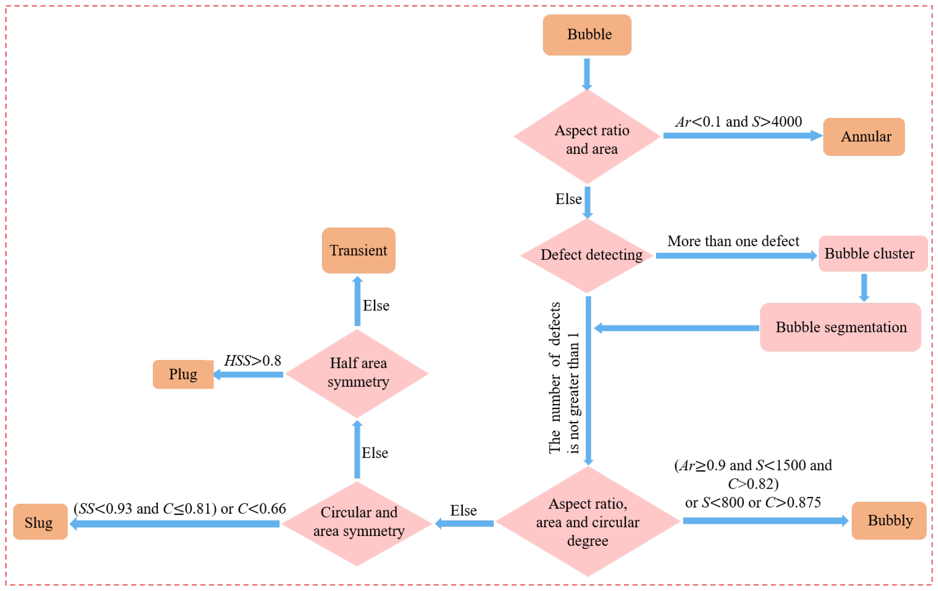
Figure 8 presents the method for flow pattern recognition based on the classification characteristics. The annular flow bubbles are distinguished by their aspect ratio and area. The bubbly flow bubbles are classified by area, roundness, and aspect ratio. The slug flow bubbles are determined by area symmetry and roundness. The transition and plug flow bubbles are differentiated by the half-area symmetry.
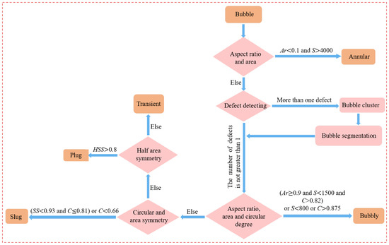
Figure 8.
Bubble flow pattern identification method.
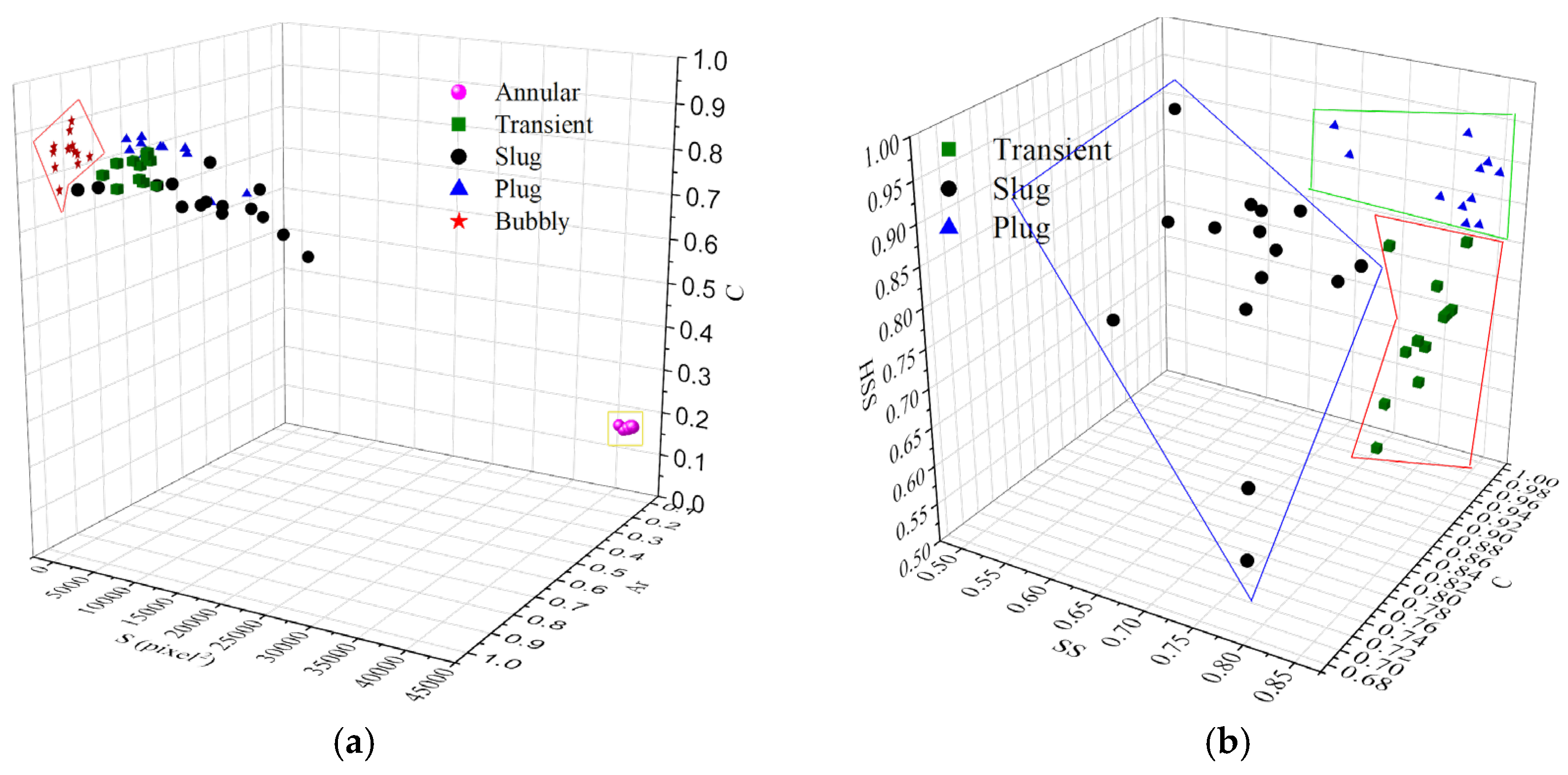
Figure 9 shows a scatter plot of the classification characteristics of each flow pattern. From Figure 9a, it can be seen that the area, aspect ratio, and roundness can distinguish annular flow and bubbly flow from the other flow patterns. Also, Figure 9b shows that roundness, area symmetry, and half-area symmetry can well determine slug flow, plug flow, and transient flow.
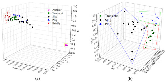
Figure 9.
The scatter diagram of bubble flow pattern recognition. (a) roundness (C); (b) half-area symmetry (HSS).
2.4. Calculation of Bubble Volume
There are two difficulties in the bubble volume calculation in the hydraulic braking pipeline, including the segmentation of bubble clusters and the application of appropriate algorithms to evaluate the volume of isolated bubbles. In this study, the watershed algorithm was used to segment the bubble clusters. The bubble volume was approximated to the volume of the rotating body by the numerical integration method.
2.4.1. Improved Watershed Algorithm
Methods such as Hough transform [26], watershed algorithm [17,27], breakpoint detection [28], and the edge pixel gradient algorithm [29] have been used to segment bubble clusters. But, among these methods, the Watershed algorithm has the best universality and strong applicability to different bubble morphology and different ranges of image pixel gradients [30]. Therefore, the watershed algorithm was adopted in this study to segment bubble clusters.
In this study, a grayscale image is generated according to the shortest distance between each pixel point and the bubble contour, as shown in Figure 10. In Figure 10, the pixels closer to the bubble contour have higher pixel values, and the Watershed algorithm was applied to complete the bubble group segmentation accurately.
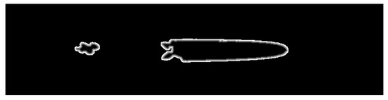
Figure 10.
A grayscale image according to the shortest distance between the pixel point and bubble contour.
2.4.2. Bubble Segmentation
As Figure 11 shows, the bubbles are in contact with each other. To calculate its volume, specific methods should be developed to divide the overlapping bubbles into isolated bubbles.
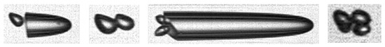
Figure 11.
Bubble cluster.
In this study, contour defects were used to distinguish the bubble clusters from isolated bubbles, and different bubble segmentation methods were used for two-bubble clusters and multiple-bubble clusters (the bubble cluster involving more than two bubbles), respectively. The specific segmentation process is enumerated in Table 1.

Table 1.
Bubble segmentation process.
Table 1.
Bubble segmentation process.
|
|
|
|
|
|
|

Figure 12.
Bubble segmentation. (a) Binarization picture of multiple bubbles; (b) binarization picture of two-bubble cluster; (c) bubble cluster extracted from (a); (d) bubble cluster extracted from (b); (e) bubble cluster after internal filling from (c); (f) bubble interior profile for (c).
Figure 12.
Bubble segmentation. (a) Binarization picture of multiple bubbles; (b) binarization picture of two-bubble cluster; (c) bubble cluster extracted from (a); (d) bubble cluster extracted from (b); (e) bubble cluster after internal filling from (c); (f) bubble interior profile for (c).
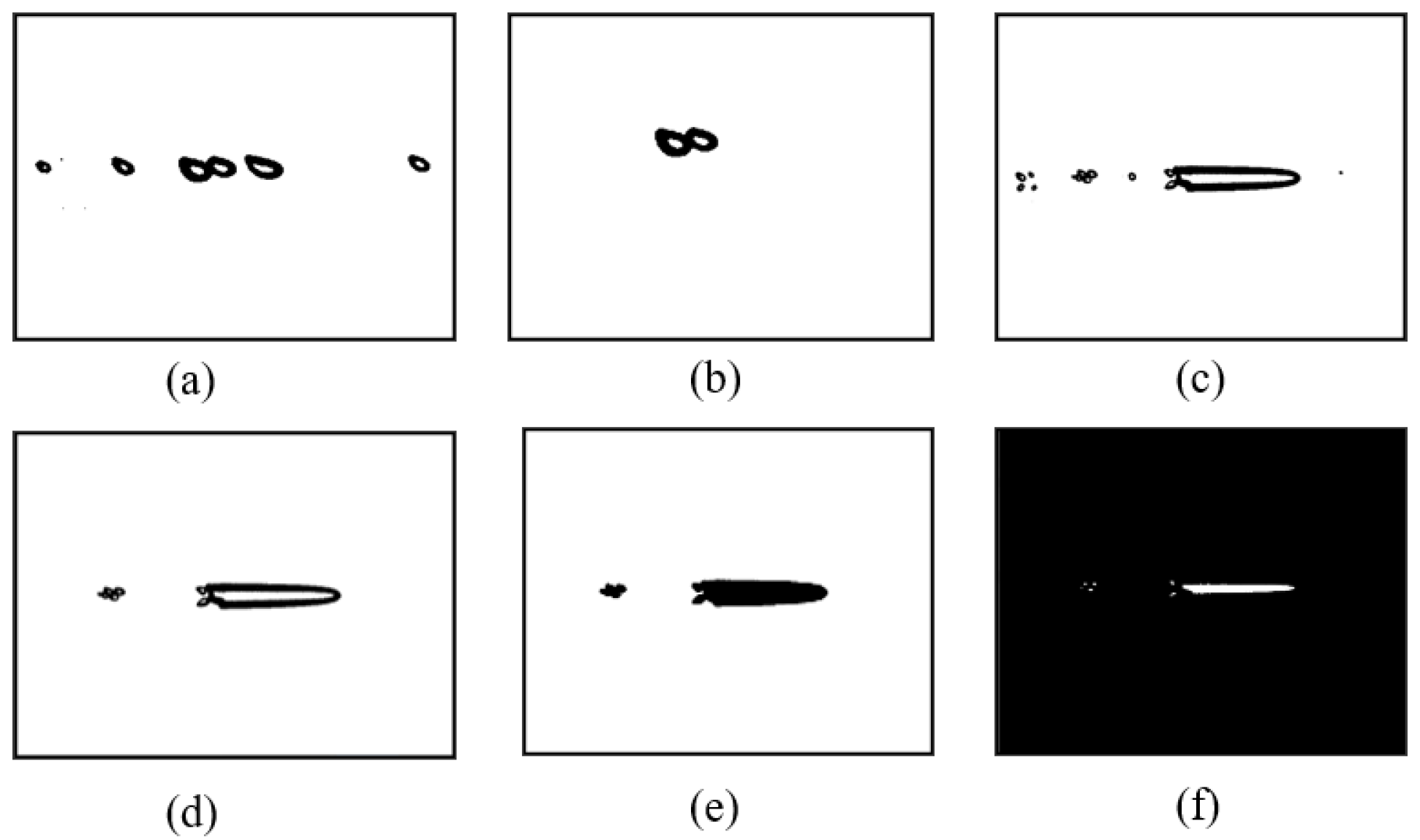
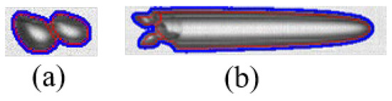
Figure 13.
Results of bubble segmentation. (a) Results of bubble segmentation for the two-bubble cluster; (b) results of bubble segmentation for the multiple-bubble cluster.
Figure 13.
Results of bubble segmentation. (a) Results of bubble segmentation for the two-bubble cluster; (b) results of bubble segmentation for the multiple-bubble cluster.

2.4.3. Volume Calculation Method of Isolated Bubble
For bubbles with relatively regular shapes, some studies used the volume formula of a sphere or an ellipsoid to solve the bubble volume [31]. For bubbles with complex shapes, researchers used the complete matching method based on a virtual stereo vision to reconstruct the bubbles in three dimensions. This method uses one mirror so that a camera can capture images of bubbles at different angles and carries out a three-dimensional reconstruction of complex bubbles based on the captured images [32,33]. In this study, the bubbles are approximated as rotating bodies (shown in Figure 14), and the bubble volume is calculated by Equation (1).
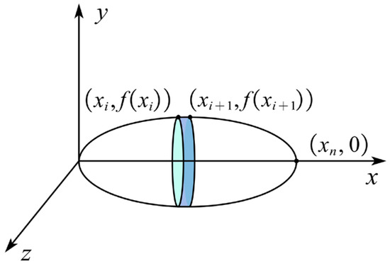
Figure 14.
Integral diagram.
2.5. Bubble Tracking Method
2.5.1. Hungarian Algorithm
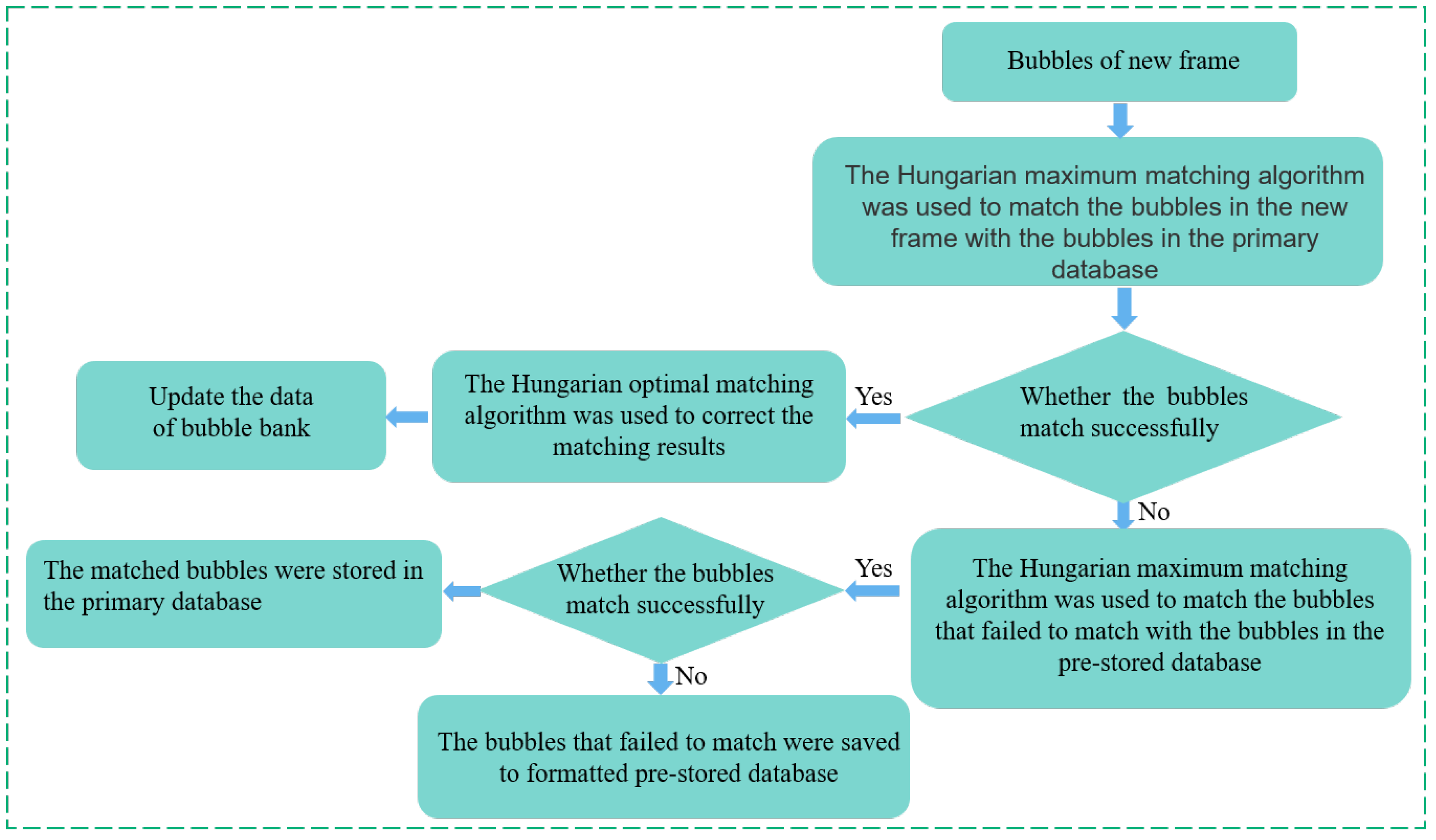
Maximum matching [34] and optimal matching [35] are the types of Hungarian algorithms. The maximum matching can obtain a matching method with the maximum number of matching groups between two groups of variables. The optimal matching is determined based on the consumption matrix to minimize the total cost of matching. In the tracking algorithm of this study, the Hungarian maximum matching algorithm was first used to find bubbles with similar characteristics in the new frame. The Hungarian optimal matching algorithm was then used to find the most reasonable matching scheme.
2.5.2. Matching Characteristics
The matching characteristics of the Hungarian algorithm have to be extracted to show if two bubbles are allowed to match the matching effect. Three matching characteristics of bubble horizontal position m, bubble lengthwise position n, and bubble area S was proposed in this study.
- (1)
- Match admission threshold
Before the Hungary maximum matching algorithm is performed, it is necessary to ascertain whether the object and target can be matched. The thresholds for the horizontal position deviation , the lengthwise position deviation , and the area deviation are determined. Matching between two bubbles is permitted when the deviation of each matching characteristic between the two bubbles is within the matching admission threshold.
- (2)
- Characteristic distance
In this study, the Hungarian optimal matching algorithm requires a parameter to measure the matching effect between the bubbles. A shorter characteristic distance between two bubbles indicates a higher similarity and a higher matching degree. Equations (2)–(4) express the characteristic distances of three matching characteristics.
The above parameters are used to quantitatively express the similarities between bubbles by using the significant shape characteristics of large bubbles and the significant position characteristics of small bubbles. The weighted values of the three characteristic distances are used as the loss values between bubbles. The Hungarian optimal matching algorithm is proposed based on a loss matrix composed of the loss values.
2.5.3. Implementation of Bubble Tracking
For bubble tracking, a pre-stored database and a primary database are established. The pre-stored database stores the parameters for the bubbles that are detected for the first time. The primary database stores the parameters for the bubbles that are tracked. The instantaneous velocity of the tracked bubbles is calculated using the bubble position deviation and the time difference between two frames, and the next location of tracked bubbles is predicted. The life cycle of tracked bubbles (the number of frames that bubbles are tracked) is calculated during the process of bubble tracking. During tracking, if a bubble with a life cycle of less than 4 fails to match in a frame, its relevant parameters will be deleted from the primary database. If a bubble with a life cycle of not less than 4 fails to match in a frame, its vanishing period is calculated, and its position in each frame is predicted to match in each subsequent frame. If the vanishing period of the bubble is greater than 60 or its predicted position is beyond the window range, the relevant parameters of this bubble would be deleted from the primary database. This matching process can increase the stability of bubble tracking. The matching process of bubbles in the bubble tracking process is shown in Figure 15.
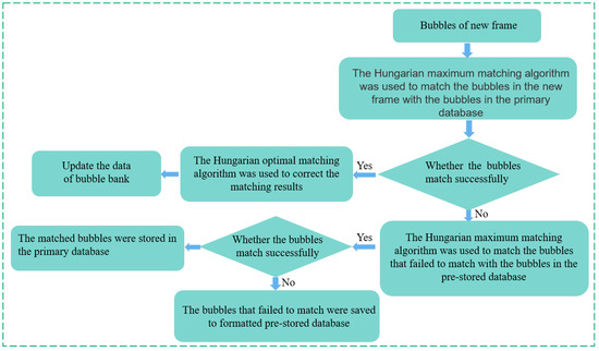
Figure 15.
Matching flow chart.
2.6. Error Analysis
2.6.1. Error Analysis of Bubble Flow Pattern Recognition
To test the accuracy of the bubble flow pattern recognition, 50 test datasets were substituted into the flow pattern identification rule to predict the flow pattern. Only one transition bubble in the 50 test datasets was misidentified as a plug flow bubble. The accuracy of the bubble flow pattern recognition method based on the bubble shape characteristic reached up to 98%. The recognition speed was fast and real-time. Only a small number of training set samples were needed to determine the bubble characteristic threshold.
2.6.2. Integral Error of the Bubble Volume Calculation
There is a truncation error in the calculation of bubble volume by using the compound trapezoidal formula. The remainder term of the compound trapezoidal formula is expressed as:
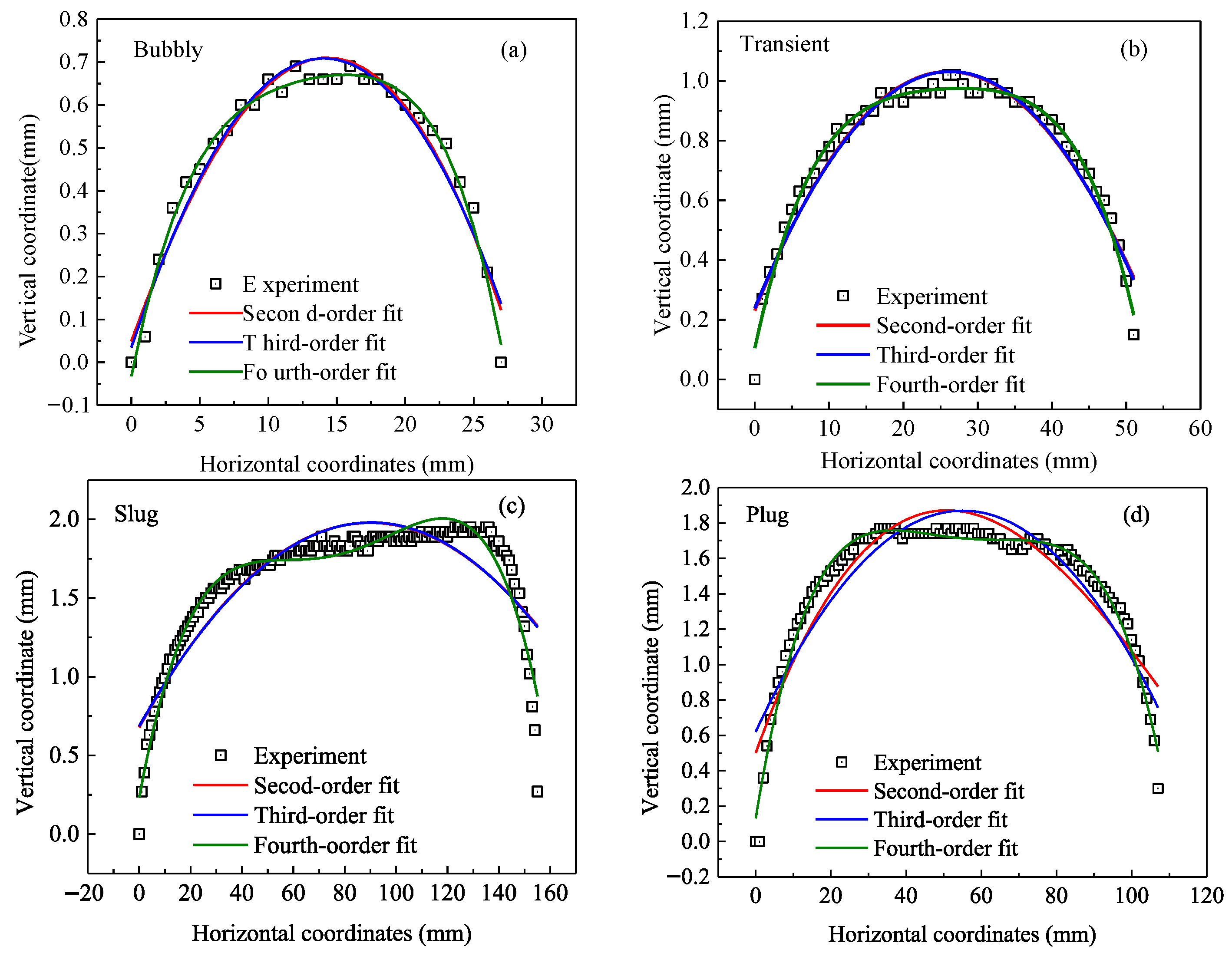
where is the function of the integral curve, and is the abscissa of the rightmost point of the bubble contour. The [0,] area is divided into equal parts for integration. The length of each integral region is . The bubble contours in this study were discrete sampling points. The derivative value of the curve at each point is required by calculating the residual term. To observe the error of quadrature by the compound trapezoidal formula for bubble contours of each flow pattern, four bubble contours of different bubble flow patterns were fitted polynomially. As seen in Figure 16, the fitting effect of the fourth-order polynomial is good. The fitting coefficients and fitting residuals are summarized in Table 2.
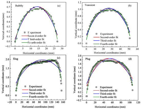
Figure 16.
Bubble contour fitting diagram.
Table 2.
Fitting coefficient.
The above four fourth-order polynomials were used to solve the volume integral remainder of the flow bubbles. When in Equation (5) was maximum, the integral errors in Table 3 were obtained. From each remainder value, it could be seen that the maximum integration error using the compound trapezoidal formula to integrate the bubble contour of the nearly fourth-order curve is within 1%, showing that the accuracy of the integration is satisfactory.
Table 3.
Integral error.
2.6.3. Error Analysis of Bubble Tracking
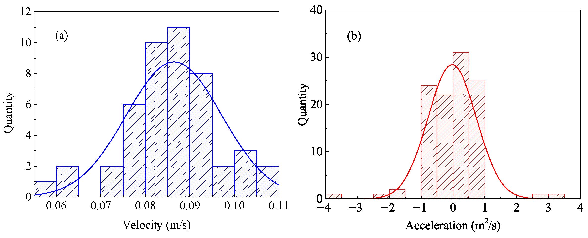
There were similar, occluded, or extremely small bubbles in the bubble matching process, which caused the wrong matching of the bubbles. The bubble velocity and bubble acceleration do not change suddenly when the bubble moves in the pipeline. Therefore, when the velocity or acceleration of a bubble deviates too much from its average velocity or acceleration in a frame, it is determined that the bubble has error tracking in this frame. The velocity and acceleration distributions of different bubble samples with the same serial number are shown in Figure 17. Based on the characteristics of bubble velocity and acceleration, the 3 norm or the t-test norm could be used to eliminate the mismatched bubbles.
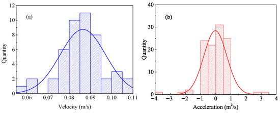
Figure 17.
Bubble velocity and acceleration distribution with the same serial number. (a) velocity; (b) acceleration.
For bubbles with a sample number less than or equal to 10 and larger than 10, the t-test norm and 3σ norm are used to eliminate bubble samples with abnormal velocity or acceleration. The bubbles in the two-phase flow videos at 11 vehicle speeds were screened using the above criteria. Finally, 3456 bubble samples were eliminated from the 269,483 bubble samples. The rejection ratio was 1.283%. The accuracy of bubble tracking was relatively high.
3. Experimental Results
3.1. Bubble Flow Pattern
The bubbles were divided into six flow patterns: bubble cluster, bubbly flow bubble, slug flow bubble, plug flow bubble, transient flow bubble, and annular flow bubble. The recognition method for each flow pattern was proposed. Some bubbles experienced a variety of flow patterns as they flowed through the photo window. The evolution of the flow pattern in the window was observed and its proportion was calculated. Table 4 shows the proportion of bubbles of each flow type at each wheel speed, while Table 5 lists the proportion of bubbles in unsteady flow for each flow pattern.
Table 4.
Proportion of bubbles of each flow pattern at each wheel speed.
Table 5.
Proportion of bubbles in unsteady flow for each flow pattern.
As shown in Table 4, the occurrence frequency of bubbly flow in the hydraulic braking pipeline is the largest, followed by slug flow. Transient flow and plug flow occurrence frequencies are very low. The annular flow is observed at a low wheel speed of 200 r/min. The possible reason is that at low speeds, due to the relatively extended duration, bubbles tend to accumulate around the pipeline while liquid remains at the center, thus forming annular flow. Table 5 shows that bubbles in plug and transient flow exhibit low stability, rapidly transitioning to other flow patterns. The stability of slug flow is better than that of the first two flow patterns, but the slug flow bubbles with flow pattern conversion in the window still account for 71.5% of the total number of slug flow bubbles. The flow pattern of the cluster is unstable because the bubbles in the cluster will always separate and merge in the process of movement. Bubbly flow has the highest stability because of their small volume.
3.2. Bubble Volume
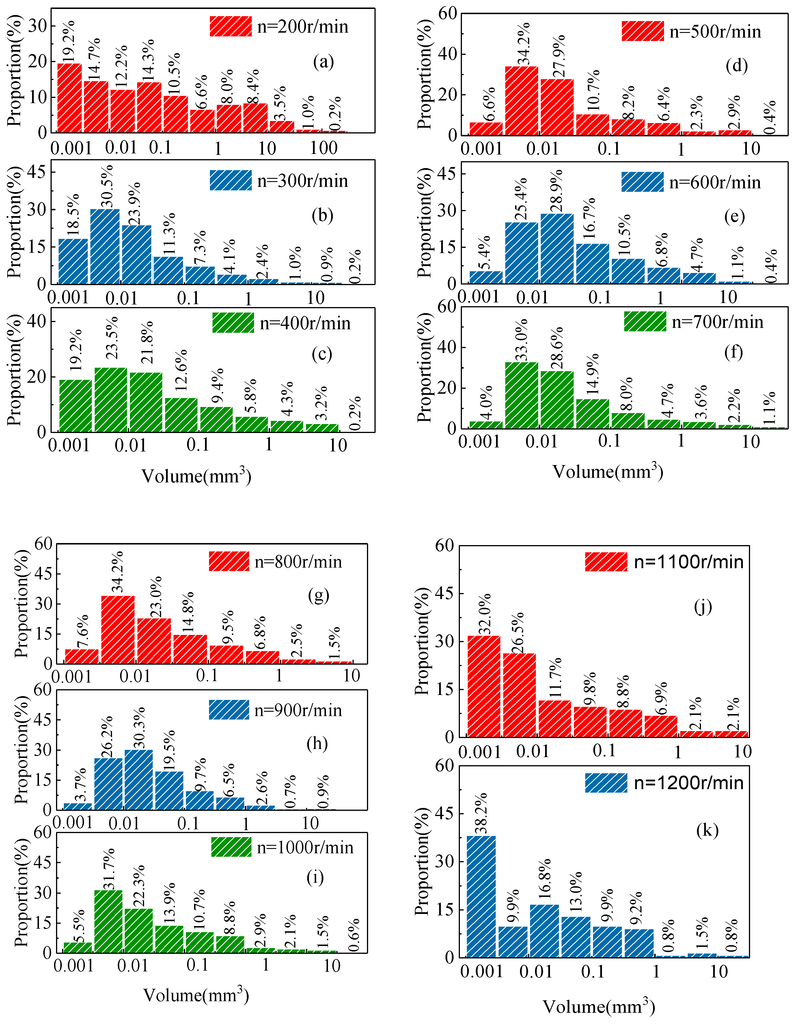
The volume of bubbles that appeared in the hydraulic braking pipeline was as small as ten minus cubic millimeters and as large as hundreds of cubic millimeters. Statistics of the bubble volume distribution at different wheel speeds are shown in Figure 18.

Figure 18.
Bubble volume distribution at different wheel speeds.
Figure 18 shows that the proportion of small-volume bubbles in the hydraulic braking pipeline is relatively high. The volume of the bubbles is generally concentrated within 0.001–1 mm3. As the wheel speed increases, the proportion of small volume bubbles in the pipe first decreases, then increases. This is because the pressure in the pipe increases with the increase in the wheel speed. However, as the pressure in the pipe increases, some small volume bubbles dissolve into the brake fluid, reducing the proportion of small volume bubbles in the pipe. With the further increase in pressure in the pipeline, some large volume bubbles break into small volume bubbles, raising the proportion of small volume bubbles in the pipeline.
3.3. Velocity of Bubbles
3.3.1. Velocity Distribution of Bubbles in the Transparent Pipe
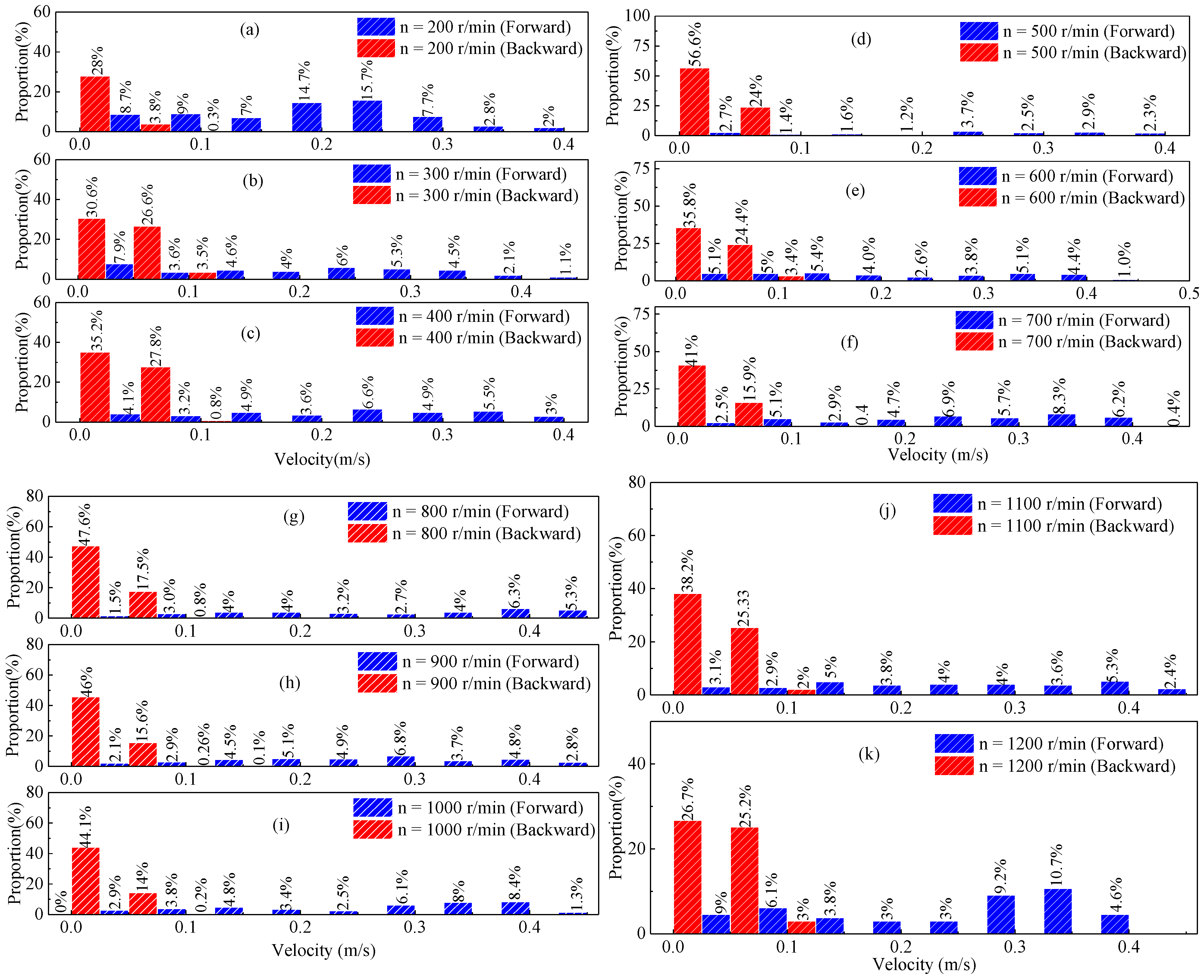
The bubble was tracked to obtain the bubble velocity. The velocity of the bubble reflects the movement of the bubble and the flow state of the two-phase flow. The average velocity of a single bubble in the entire flow process in the window was used as the bubble velocity. The velocity distribution of the bubbles at different wheel speeds is shown in Figure 19.
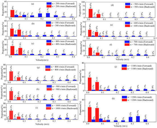
Figure 19.
Bubble velocity distribution at different wheel speeds.
Figure 19 shows that the bubble velocity in the hydraulic braking pipeline is between −0.15 m/s and 0.45 m/s. The bubbles that move in the opposite direction between −0.05 m/s and 0 m/s have the highest proportion in the pipeline at each wheel speed. As can be seen from Figure 19, the bubble velocity of reverse movement in the pipeline is generally within 0.1 m/s, while the bubble velocity of forward movement is more than 0.4 m/s. This is because the backflow pressure difference in the hydraulic brake pipe is much smaller than the brake pressure difference, which causes the forward movement of bubbles under the action of a large pressure difference to accelerate to a higher speed.
3.3.2. Velocity Distribution of Bubbles
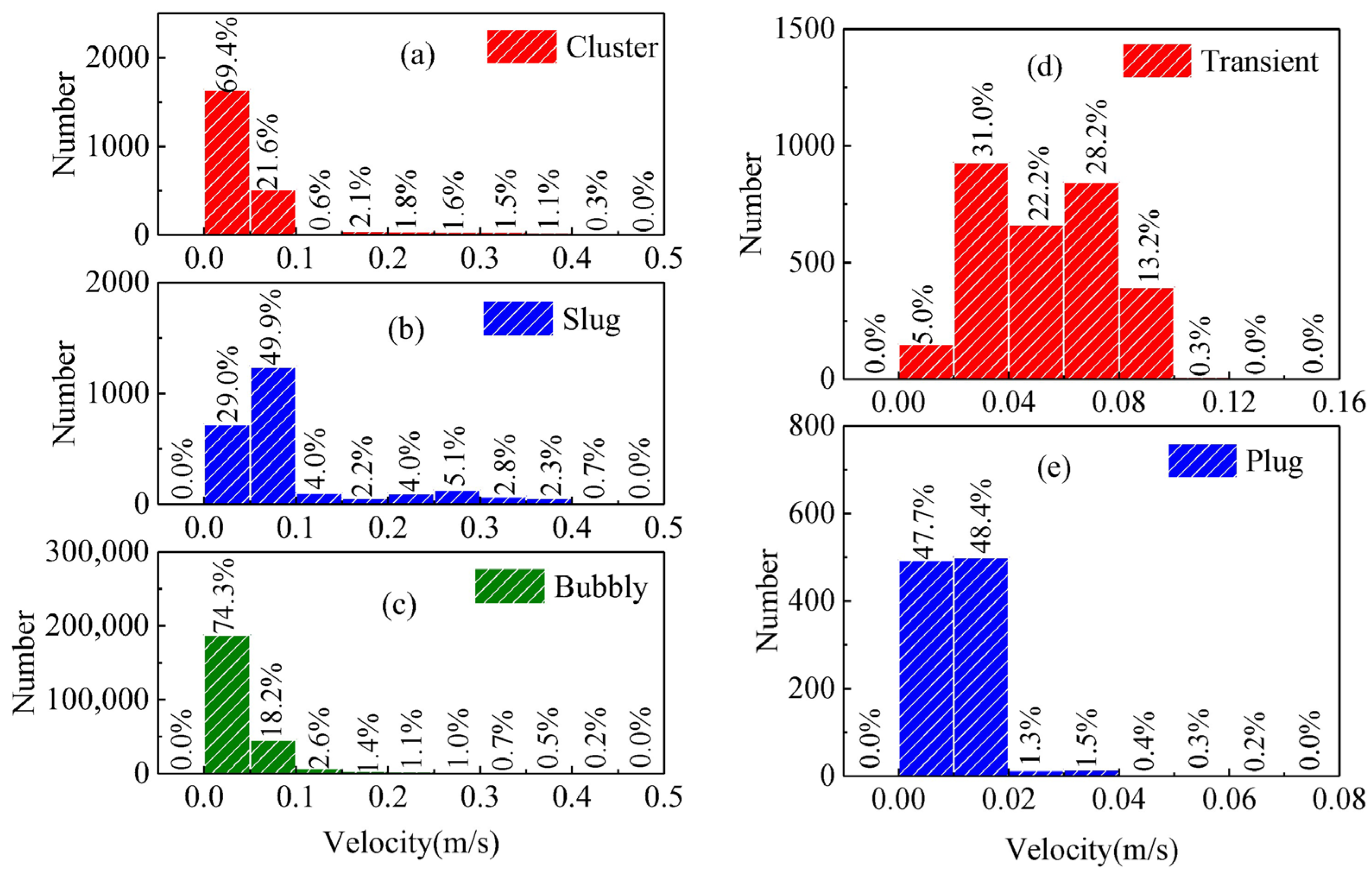
The bubble flow pattern is closely related to its motion. Figure 20 plots the velocity distributions of five flow patterns under 11 wheel speeds. As Figure 20 shows, the velocity distribution extent of bubbly flow bubbles, slug flow bubbles, and bubble clusters is relatively wide. Figure 20 indicates that the velocity distribution extent of slug flow bubbles is the widest, and the proportion of high-speed bubbles in the two-phase flow of this flow pattern is the highest. The velocity distribution extent of the plug flow and transient flow bubbles is extremely narrow. Most of the plug flow bubbles have a velocity of 0–0.02 m/s, and the maximum velocity of the plug flow bubbles is 0.07 m/s. The velocity distribution extent of the transient flow bubble is slightly larger than that of the plug flow bubble, and the maximum velocity is 0.12 m/s. It can be inferred that when the pressure in the pipeline is not high, the gas holdup in the pipeline is relatively large and large bubbles are easily formed. At this time, the two-phase flow has a slow flow velocity. Under gravitational effects, plug flow bubbles develop. If there is a pressure difference between the two ends of the pipeline at this time, the flow velocity increases and the plug flow bubbles continue to accelerate. Gradually, it evolves into transient flow bubbles and metamorphoses into slug flow bubbles at a high flow rate. The formation of bubbly flow bubbles is related to the local gas holdup in the pipeline. The flow pattern of bubbly flow bubbles will not change with the fluctuation of the pipeline pressure difference. Therefore, the velocity distribution of bubbly flow bubbles is very wide.
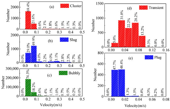
Figure 20.
Velocity distribution of bubbles with different flow patterns.
3.3.3. Average Velocity of Different Volume Bubbles
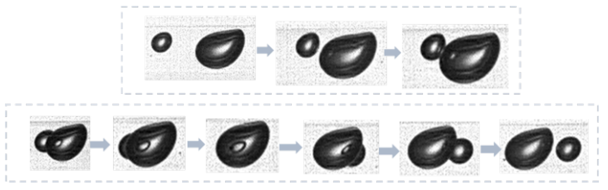
In the video of the two-phase flow, many large bubbles exceeded small bubbles or collided with small bubbles, as shown in Figure 21. Therefore, this section discusses the relationship between bubble volume and bubble velocity.
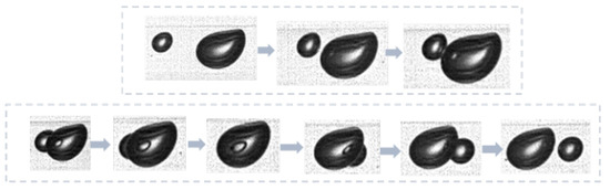
Figure 21.
Bubble chasing in the pipeline.
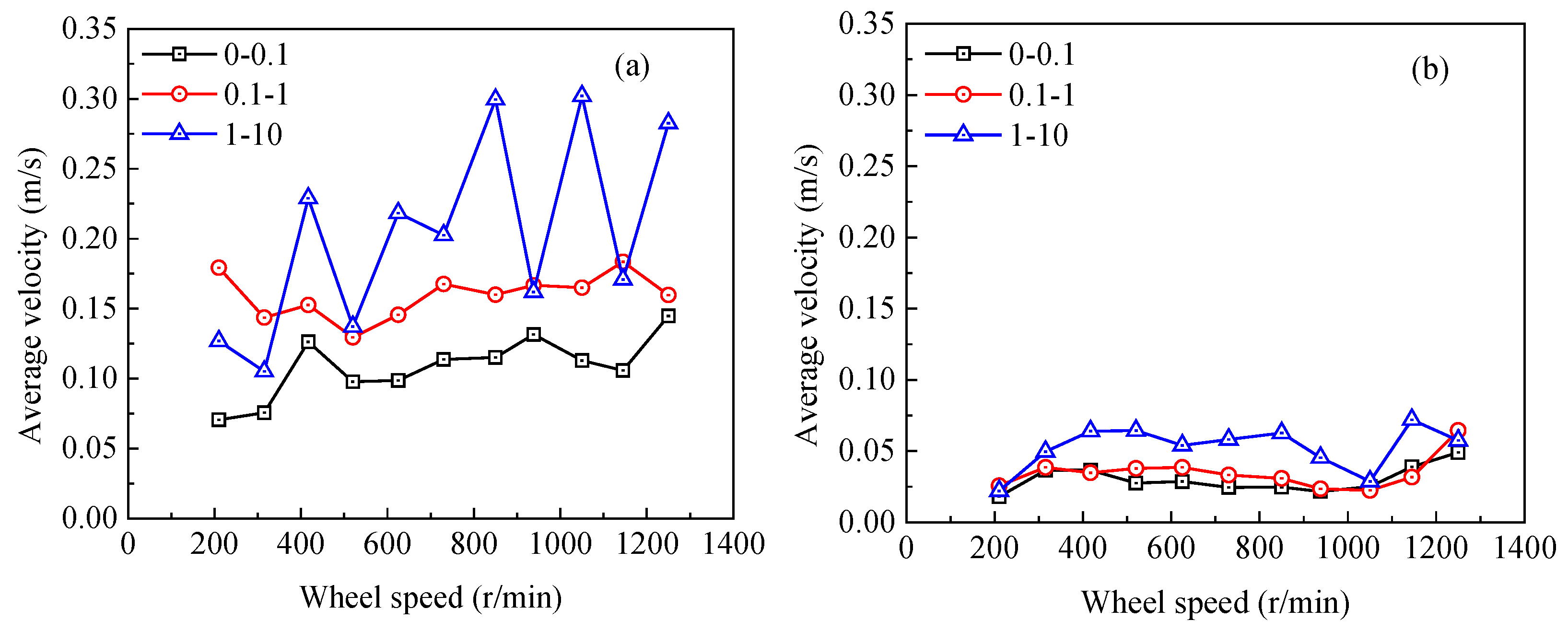
The average velocity of bubbles in different volume ranges was calculated (0–0.1 mm3, 0.1–1 mm3, and 1–10 mm3), as displayed in Figure 22.
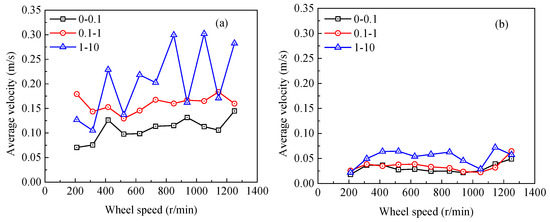
Figure 22.
Average velocity of bubbles at different volumes. (a) forward; (b) backward.
The average velocity of large-volume bubbles is greater than that of small-volume bubbles. The average velocity of forward-moving bubbles is greater than the average velocity of reverse-moving bubbles, as shown in Figure 22a,b.
4. Further Discussion
4.1. Distribution of Bubbles
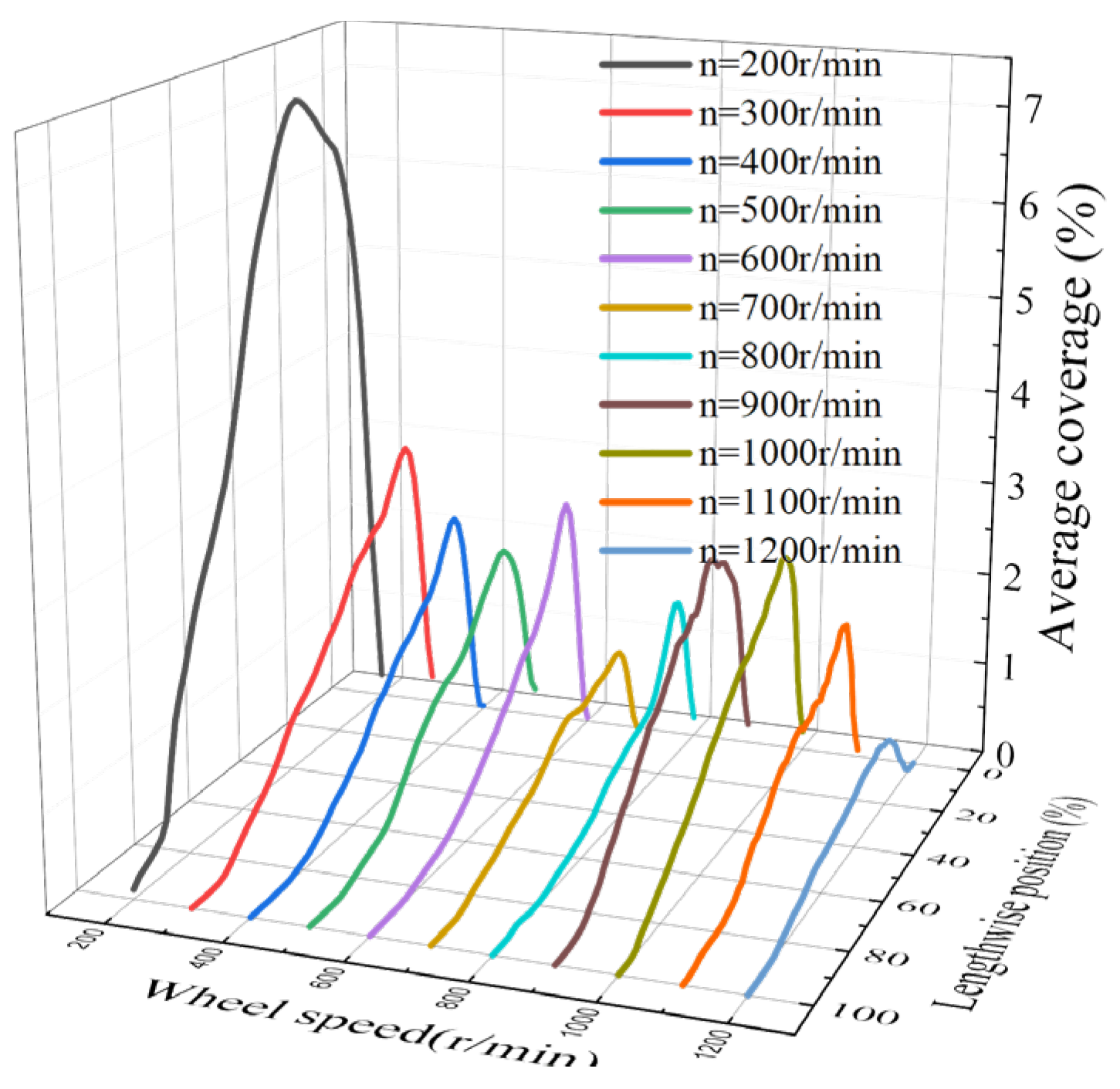
The pixels inside the bubbles in each frame of the images are termed as covered pixels. The frame-wise occupancy that each pixel in the window is covered by bubbles is defined as the coverage rate. Since bubbles mostly move in a straight line in the pipeline, the distribution of bubbles in the vertical direction is considered. The pixels covered in the horizontal direction of the pipeline are averaged to obtain the average coverage rate. The average coverage rate indicates the probability of bubbles appearing in each position of the hydraulic braking pipeline in the longitudinal direction. It also reflects the concentration of bubbles in the longitudinal distribution of the hydraulic braking pipeline. The longitudinal position of the pipeline is divided into 100 equal parts as the x-axis of the statistical graph in Figure 23. Moreover, the average coverage is the y-axis of the graph, as shown in Figure 23.
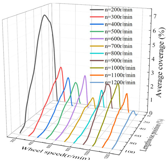
Figure 23.
Average bubble coverage in the longitudinal direction of the pipeline.
According to Figure 23, the peak of average coverage always appears in the middle and upper parts of the pipeline. Most of the bubbles are concentrated in the position of 10–20% from the top-down of the pipeline. Bubbles at the 200 r/min wheel speed have a wider distribution of locations in the vertical direction due to the larger bubble size. The peak value of the average coverage rate at 200 r/min is about 40% from the top-down of the pipeline, and the average coverage rate of the entire longitudinal pipeline is relatively large. Increasing wheel speed elevates brake pressure while reducing gas holdup in the pipeline and lowering peak average coverage. Furthermore, under the action of inertial force, the bubble does not have time to float up to reach the position of the pipeline wall. So, as the wheel speed increases, the average coverage rate peak gradually moves down. Until the wheel speed of 1200 r/min, the peak of the average coverage rate appeared at approximately 25% from the top to the bottom of the pipeline.
4.2. Average Gas Holdup of Observation Window
The gas holdup in gas–liquid two-phase flow will directly affect the performance and safety of equipment. According to the total volume of bubbles and the volume of pipes in the observation window, the observation window gas holdup in each frame image can be calculated. By averaging the gas holdup of each frame in the whole video, the average gas holdup can be determined. The formula for obtaining the average gas holdup is:
where is the number of video frames, is the number of bubbles in each frame, r is the inner radius of the transparent pipe, and is the window width. Hence, the average gas holdup of the forward and reverse flows in the hydraulic braking pipeline can be obtained. As shown in Figure 24, the average gas holdup of forward flow is higher than the average gas holdup of reverse flow in the pipeline at low wheel speed, but the average gas holdup of forward flow is generally lower than the average gas holdup of reverse flow in the pipeline as the wheel speed increases. This is due to the positive braking pressure increasing with the increasing wheel speed of the vehicle, leading to bubbles merging into the brake fluid. Therefore, the gas holdup of the positive flow brake fluid continues to decrease.
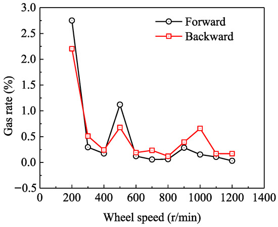
Figure 24.
Average gas holdup in observation window.
4.3. Bubble Acceleration Analysis
The real-time position and velocity of the bubbles can be used to obtain the real-time acceleration of the bubbles. The acceleration represents the bubble’s inertial force. Figure 25 presents the acceleration distribution of bubbles with different bubble flow patterns. The bubble acceleration in the pipeline is between 0–4 m/s2. The high acceleration of slug flow bubbles, bubbly flow bubbles, and bubble clusters accounts for a relatively large proportion. The proportion of high acceleration of plug flow and transient flow bubbles is much smaller. Bubbles with different velocities collide to form a bubble cluster, which will have a relatively large acceleration under the action of inertial. So, the bubble clusters have the highest proportion of large acceleration. Presumably, the acceleration of bubbles in the pipeline is changeable and intermittent. Figure 26 depicts the evolution of bubble velocity and acceleration during bubble acceleration phases. The uneven turntable surface induces fluctuating bubble acceleration, resulting in undulating velocity. Despite this kinematic instability, bubble morphology remains stable due to delayed feedback.
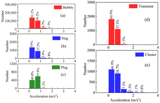
Figure 25.
Acceleration distribution of bubbles with different bubble flow patterns.
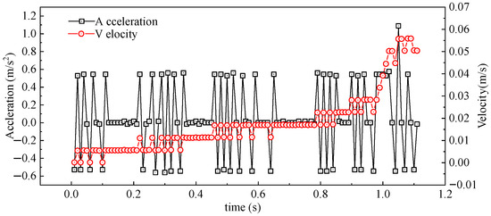
Figure 26.
Evolution of velocity and acceleration of an accelerating bubble.
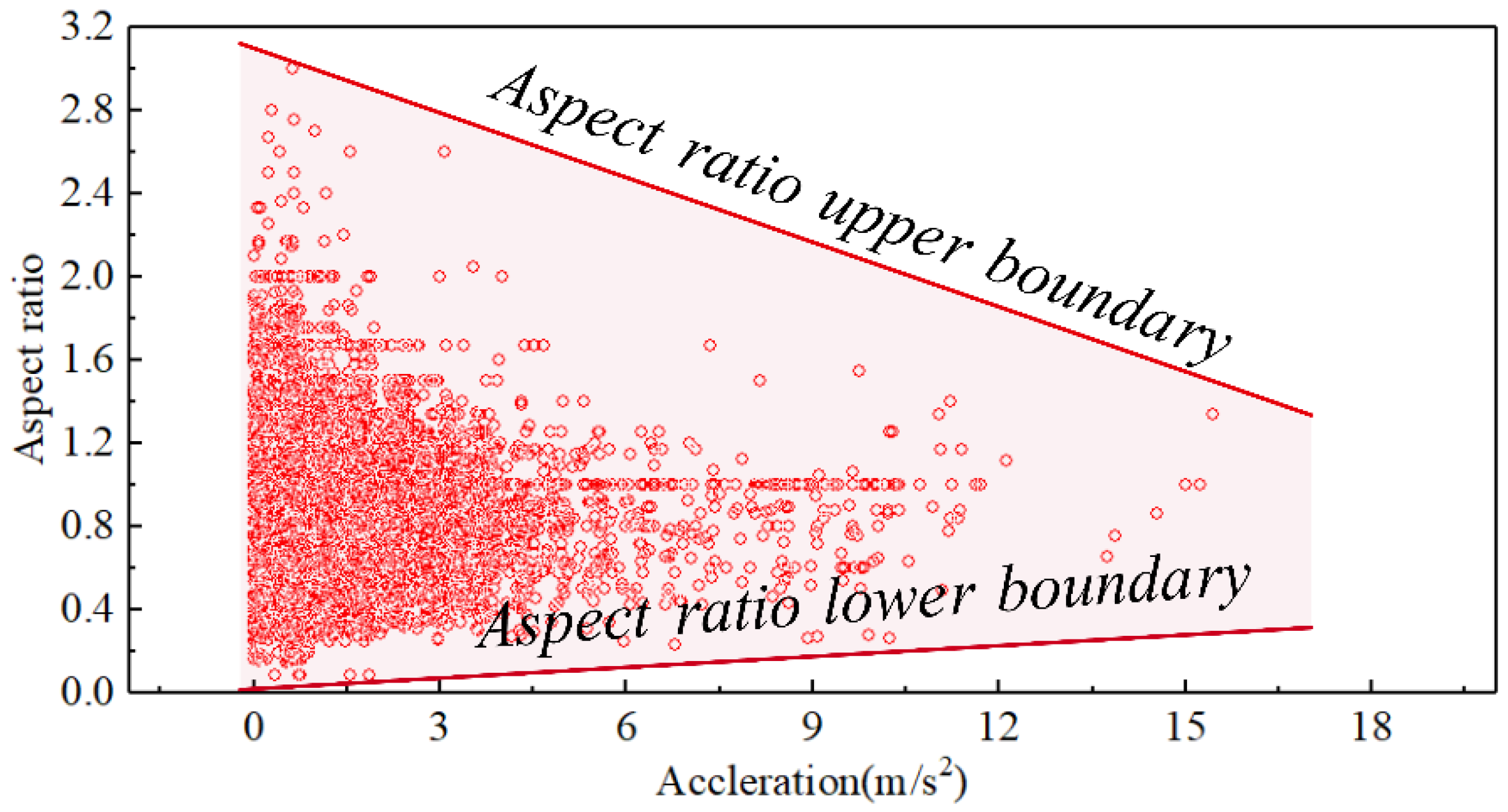
The aspect ratio is an important parameter that reflects the stress condition of the bubble [36,37]. The scatter plot of bubble acceleration and aspect ratio is provided in Figure 27. The figure shows that the bubble aspect ratio has a wide distribution range when the bubble acceleration is relatively small. The main reason is that the bubble acceleration exists in the form of fluctuation and the change of bubble shape is delayed by the change of bubble force. Increasing acceleration narrows the bubble aspect ratio distribution: its upper bound decreases while the lower bound rises, converging toward unity. This is because, with the increase in acceleration, the large bubbles with a small aspect ratio in the pipeline break into small bubbles, which increases the aspect ratio of the bubbles, and the small bubbles with a large aspect ratio in the pipeline dissolve into the liquid. Eventually, the aspect ratio of bubbles in the pipeline tends to be one.
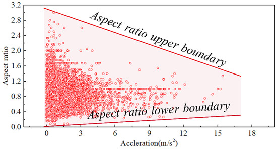
Figure 27.
Scatter plot of aspect ratio versus acceleration.
It is worth noting that temperature strongly affects bubble dynamics in brake fluid. Heat from the ambient, cyclic braking compression, engine and body dissipation, and brake-pad friction all raise the fluid’s temperature. How this heating alters bubble behavior remains an open question for future work.
5. Conclusions
This study investigated the gas–liquid two-phase flow in a hydraulic braking pipeline. The bubble flow pattern of bubbles was analyzed using the bubble morphological features. At all tested wheel speeds, bubbly flow was predominant, followed by slug flow, and other patterns occurred in negligible proportions. Plug and transient flows exhibited significant shape instability, rapidly evolving into other flow patterns.
The bubbles were segmented to calculate the bubble volume using the numerical integration method to quantify the bubble volume distribution across wheel speeds. As the wheel speed increased, the proportion of small-volume bubbles initially decreased and then increased. Time-resolved tracking captured bubble kinematics. The results indicated that the velocity of the bubble in the forward flow was greater than that in the reverse flow. Moreover, the bubble velocity increased with increasing wheel speed. The relationship between bubble volumes, bubble flow patterns, and bubble velocity was investigated. The results revealed that the transient flow and plug flow bubbles were mostly at a low speed. The velocity of large-volume bubbles was greater than that of small-volume bubbles.
In addition, the longitudinal distribution of bubbles in the hydraulic braking pipeline was analyzed. Bubbles concentrated primarily in the upper pipeline regions, though this distribution shifted downward with increasing wheel speed. The average gas holdup of the observation window was determined using the volume of each bubble. The average gas holdup of the reverse flow was higher than that of the forward flow, but the gas holdup in the pipeline decreased with increasing wheel speed. The acceleration fluctuation state of the bubble movement was also assessed, as well as, the relationship between the bubble aspect ratio and the bubble acceleration. High-acceleration bubbles consistently exhibited aspect ratios approaching 1.
Author Contributions
Conceptualization, X.L. and C.X.; methodology, Y.K.; software, Y.K.; validation, Y.K., J.S. and M.L.; formal analysis, X.L.; investigation, Y.K.; resources, X.L.; data curation, Y.K.; writing—original draft preparation, X.L.; writing—review and editing, C.X.; visualization, Y.K.; supervision, X.L.; project administration, X.L.; funding acquisition, X.L. All authors have read and agreed to the published version of the manuscript.
Funding
This research was funded by the Natural Science Foundation of Zhejiang Province, grant number LZ23E060002 and LY14E05002, and The APC was funded by the Natural Science Foundation of Zhejiang Province.
Data Availability Statement
The original contributions presented in the study are included in the article, further inquiries can be directed to the corresponding authors.
Conflicts of Interest
The authors declare no conflict of interest.
References
- Xue, M.H.; Fu, Y.; Geng, X.H.; Sun, S.H.; Lei, Y.L. Integration analysis model of oil-charging system about parallel hydraulic retarder and its response characteristic. Eng. Sci. Technol. Int. J. 2024, 53, 101685. [Google Scholar] [CrossRef]
- Zhang, R.C.; Yu, X.; Hu, Y.L.; Zang, H.J.; Shu, W. Active control of hydraulic oil contamination to extend the service life of aviation hydraulic system. Int. J. Adv. Manuf. Technol. 2018, 96, 1693–1704. [Google Scholar] [CrossRef]
- Hunter, J.E.; Cartier, S.S.; Temple, D.J.; Mason, R.C. Brake fluid vaporization as a contributing factor in motor vehicle collisions. SAE Trans. 1998, 107, 867–885. [Google Scholar]
- Jun, K.J.; Park, T.W.; Jung, S.P.; Lee, S.H.; Yoon, J.W. Development of a numerical method to predict the alpine test result. Proc. Inst. Mech. Eng. Part D J. Automob. Eng. 2008, 222, 1841–1849. [Google Scholar] [CrossRef]
- Wang, X.Y.; Zhang, Z.; Li, Y.L. Analysis of water coolant pressure fluctuation induced by piston slap. Eng. Fail. Anal. 2020, 112, 104382. [Google Scholar] [CrossRef]
- Wang, Y.; Chen, Y.; Li, X.; Xu, C.; Wei, W.; Zhao, J.; Jin, J.; Oppong, F. Spatiotemporal evo- lution of gas in transmission fluid under acoustic cavitation conditions. Appl. Sci. 2024, 14, 6233. [Google Scholar] [CrossRef]
- Chang, Y.J.; Xu, Q.; Zou, S.F.; Zhao, X.Y.; Wu, Q.H.; Wang Thévenin, D.; Guo, L.J. Experiments and predictions for severe slugging of gas-liquid two-phase flows in a long-distance pipeline-riser system. Ocean. Eng. 2024, 301, 117636. [Google Scholar] [CrossRef]
- Le, T.-L.; Chen, J.-C.; Nguyen, H.-B. Numerical study of the thermocapillary droplet migration in a microchannel under a blocking effect from the heated wall. Appl. Therm. Eng. 2017, 122, 820–830. [Google Scholar] [CrossRef]
- Deng, H.W.; Zhang, C.B.; Xu, G.Q.; Tao, Z.; Zhu, K.; Wang, Y.J. Visualization experiments of a specific fuel flow through quartz-glass tubes under both sub- and supercritical conditions. Chin. J. Aeronaut. 2012, 25, 372–380. [Google Scholar] [CrossRef]
- Thaker, J.; Banerjee, J. On intermittent flow characteristics of gas-liquid two-phase flow. Nucl. Eng. Des. 2016, 310, 363–377. [Google Scholar] [CrossRef]
- Al-Safran, E.M. Probabilistic modeling of slug frequency in gas-liquid pipe flow using the Poisson probability theory. J. Pet. Sci. Eng. 2016, 138, 88–96. [Google Scholar] [CrossRef]
- Setyawan, A.; Deendarlianto, I. The effect of the fluid properties on the wave velocity and wave frequency of gas-liquid annular two-phase flow in a horizontal pipe. Exp. Therm. Fluid Sci. 2016, 71, 25–41. [Google Scholar] [CrossRef]
- Al-Kayiem, H.H.; Mohammed, A.O.; Al-Hashimy, Z.I.; Time, R.W. Statistical assessment of experimental observation on the slug body length and slug translational velocity in a horizontal pipe. Int. J. Heat Mass Transf. 2017, 105, 252–260. [Google Scholar] [CrossRef]
- Kajero, O.T.; Abdulkadir, M.; Abdulkareem, L.; Azzopardi, B.J. Experimental study of viscous effects on flow pattern and bubble behavior in small diameter bubble column. Phys. Fluids 2018, 30, 093101. [Google Scholar] [CrossRef]
- Li, X.; Sun, J.; Xu, C.; Li, Y.; Zhang, R.; Qian, L.; Chen, Y. Visualization of bubble flow in the channel of a dimple-type embossing plate heat exchanger under different fluid inlet/outlet ports. Int. J. Heat Mass Transf. 2019, 145, 118750. [Google Scholar] [CrossRef]
- Serra, P.L.S.; Masotti, P.H.F.; Rocha, M.S.; de Andrade, D.A.; Torres, W.M.; de Mesquita, R.N. Two-phase flow void fraction estimation based on bubble image segmentation using Randomized Hough Transform with Neural Network (RHTN). Prog. Nucl. Energy 2020, 118, 103133. [Google Scholar] [CrossRef]
- Karn, A.; Ellis, C.; Arndt, R.; Hong, J. An integrative image measurement technique for dense bubbly flows with a wide size distribution. Chem. Eng. Sci. 2015, 122, 240–249. [Google Scholar] [CrossRef]
- Lau, Y.M.; Deen, N.G.; Kuipers, J.A.M. Development of an image measurement technique for size distribution in dense bubbly flows. Chem. Eng. Sci. 2013, 94, 20–29. [Google Scholar] [CrossRef]
- Honkanen, M.; Saarenrinne, P.; Stoor, T.; Niinimaki, J. Recognition of highly overlapping ellipse-like bubble images. Meas. Sci. Technol. 2005, 16, 1760–1770. [Google Scholar] [CrossRef]
- Javeed, M.A.; Ghaffar, M.A.; Ashraf, M.A.; Zubair, N.; Metwally, A.S.M.; Tag-Eldin, E.M.; Bocchetta, P.; Javed, M.S.; Jiang, X.F. Lane line detection and object scene segmentation using Otsu Thresholding and the Fast Hough Transform for intelligent vehicles in complex road conditions. Electronics 2023, 12, 1079. [Google Scholar] [CrossRef]
- Romanengo, C.; Falcidieno, B.; Biasotti, S. Hough transform based recognition of space curves. J. Comput. Appl. Math. 2022, 415, 114504. [Google Scholar] [CrossRef]
- Li, C. Dangerous posture monitoring for undersea diver based on frame difference method. J. Coast. Res. 2020, 103, 939–942. [Google Scholar] [CrossRef]
- Amoozegar, M.; Akbarizadeh, M.; Bouwmans, T. Robust and efficient FISTA-based method for moving object detection under background movements. Knowl. Based Syst. 2024, 294, 111765. [Google Scholar] [CrossRef]
- Pei, W.J.; Shi, Z.H.; Gong, K. Moving object detection in satellite videos based on an improved ViBe algorithm. Signal Image Video Process. 2024, 18, 2543–2557. [Google Scholar] [CrossRef]
- Zajec, B.; Cizelj, L.; Koncar, B. Effect of mass flow rate on bubble size distribution in boiling flow in temperature-controlled annular test section. Exp. Therm. Fluid Sci. 2023, 140, 110758. [Google Scholar] [CrossRef]
- Riquelme, A.; Desbiens, A.; del Villar, R.; Maldonado, M. Identification of a non-linear dynamic model of the bubble size distribution in a pilot flotation column. Int. J. Miner. Process. 2015, 145, 7–16. [Google Scholar] [CrossRef]
- Shao, S.Y.; Li, C.; Hong, J.R. A hybrid image processing method for measuring 3D bubble distribution using digital inline holography. Chem. Eng. Sci. 2019, 207, 929–941. [Google Scholar] [CrossRef]
- Kong, R.; Rau, A.; Kim, S.; Bajorek, S.; Tien, K.; Hoxie, C. A robust image analysis technique for the study of horizontal air-water plug flow. Exp. Therm. Fluid Sci. 2019, 102, 245–260. [Google Scholar] [CrossRef]
- Bröder, D.; Sommerfeld, M. Planar shadow image velocimetry for the analysis of the hydrodynamics in bubbly flows. Meas. Sci. Technol. 2007, 18, 2513–2528. [Google Scholar] [CrossRef]
- Zhang, W.K.; Liu, D.; Wang, C.J.; Liu, R.T.; Wang, D.Q.; Yu, L.Z.; Wen, S.M. An improved Python-based image processing algorithm for flotation foam analysis. Minerals 2022, 12, 1126. [Google Scholar] [CrossRef]
- Zhou, H.; Niu, X. An image processing algorithm for the measurement of multiphase bubbly flow using predictor-corrector method. Int. J. Multiph. Flow 2020, 128, 103277. [Google Scholar] [CrossRef]
- Zhang, T.; Qian, Y.; Yin, J.; Zhang, B.; Wang, D. Experimental study on 3D bubble shape evolution in swirl flow. Exp. Therm. Fluid Sci. 2019, 102, 368–375. [Google Scholar] [CrossRef]
- Song, Y.C.; Qian, Y.L.; Zhang, T.T.; Yin, J.L.; Wang, D.Z. Simultaneous measurements of bubble deformation and breakup with surrounding liquid-phase flow. Exp. Fluids 2022, 63, 83. [Google Scholar] [CrossRef]
- He, Y.X.; Wang, D.W.; Huang, F.H.; Zhang, R.N.; Min, L.T. A D2I and D2D collaboration framework for resource management in ABS-Assisted Post-Disaster Emergency Networks. IEEE Trans. Veh. Technol. 2024, 73, 2972–2977. [Google Scholar] [CrossRef]
- Feng, Y.L.; Ma, W.; Tan, Y.; Yan, H.; Qian, J.P.; Tian, Z.W.; Gao, A. A note on Hungarian method for solving assignment problem. Appl. Sci. 2024, 14, 1136. [Google Scholar] [CrossRef]
- Anirudh, N.V.; Behera, S.; Sahu, K.C. Coalescence of non-spherical drops with a liquid surface. Int. J. Multiph. Flow 2024, 175, 104800. [Google Scholar] [CrossRef]
- Hua, J.; Zhang, X.B.; Li, H.; Luo, Z.H. Experiment and simulation study on the effect of internals in gas-liquid bubble columns with a low aspect ratio. Ind. Eng. Chem. Res. 2024, 63, 4595–4604. [Google Scholar] [CrossRef]


Disclaimer/Publisher’s Note: The statements, opinions and data contained in all publications are solely those of the individual author(s) and contributor(s) and not of MDPI and/or the editor(s). MDPI and/or the editor(s) disclaim responsibility for any injury to people or property resulting from any ideas, methods, instructions or products referred to in the content. |
© 2025 by the authors. Licensee MDPI, Basel, Switzerland. This article is an open access article distributed under the terms and conditions of the Creative Commons Attribution (CC BY) license (https://creativecommons.org/licenses/by/4.0/).